genetic algorithm for combinatorial path planning:...

Hindawi Publishing CorporationMathematical Problems in EngineeringVolume 2011, Article ID 483643, 31 pagesdoi:10.1155/2011/483643

Research ArticleGenetic Algorithm for Combinatorial PathPlanning: The Subtour Problem

Giovanni Giardini and Tamas Kalmar-Nagy

Department of Aerospace Engineering, College Station, Texas A&M University, TX 77843, USA

Correspondence should be addressed to Tamas Kalmar-Nagy, [email protected]

Received 2 May 2010; Revised 21 October 2010; Accepted 24 February 2011

Academic Editor: Dane Quinn

Copyright q 2011 G. Giardini and T. Kalmar-Nagy. This is an open access article distributed underthe Creative Commons Attribution License, which permits unrestricted use, distribution, andreproduction in any medium, provided the original work is properly cited.

The purpose of this paper is to present a combinatorial planner for autonomous systems. Theapproach is demonstrated on the so-called subtour problem, a variant of the classical travelingsalesman problem (TSP): given a set of n possible goals/targets, the optimal strategy is soughtthat connects k ≤ n goals. The proposed solution method is a Genetic Algorithm coupled with aheuristic local search. To validate the approach, the method has been benchmarked against TSPsand subtour problems with known optimal solutions. Numerical experiments demonstrate thesuccess of the approach.

1. Introduction

To build systems that plan and act autonomously represents an important direction in thefield of robotics and artificial intelligence. Many applications, ranging from space exploration[1–4] to search and rescue problems [5, 6], have underlined the need for autonomous systemscapable to plan strategies with minimal or no human feedback. Autonomy might also berequired for exploring hostile environments where human access is impossible, for example,volcano exploration [7] or for locating victims in collapsed buildings [8, 9].

For intelligent systems, there are usually two well-separated modes of operation:the autonomous planning and scheduling of goals and actions [1, 10] and the subsequentautonomous navigation [11]. Even though autonomous navigation has vastly improvedduring the past decades, human instruction still plays a crucial role in the planning andscheduling phase [12–14].

In order to increase the capability of robotic systems to handle uncertain and dynamicenvironments, the next natural step in autonomy will be the deeper integration of these twooperational modes, that is, linking the autonomous navigation system with the planning and

2 Mathematical Problems in Engineering

scheduling component [15, 16], moving the latter onboard the agent. The ultimate objective ofthis line of research is to develop a general purpose goal planner for autonomous multiagentsystems. In this context “goals” are possible states of the system (e.g., locations on a map) and“actions” are transitions between these states. An intelligent planner/scheduler should beable to achieve a set of goals (planning phase) by computing an optimal sequence of actions(scheduling phase) so that human operators only have to define the highest-level goals forthe vehicle (also referred to as agent) [17].

For path planning involving many goals/locations, the planning phase turns into amission-level planning problem, where construction of a “route” is required [18, 19]. Thisplanning phase is at a higher level of abstraction than the classic point-to-point navigation:at this level, goals are given locations on a map, and a plan represents a sequence of theselocations to be visited. On the other hand, the low-level, point-to-point path planning isconsidered in the scheduling phase, and it is usually solved once the overall location routeis known [20]. Another important difference between high and low level motion planningis their time and length scale separation, that is, local navigation occurs at a much smallerlengths and at a much faster rate than the high level planning. Due to this separation ofscales, high level motion planning usually does not take the dynamics of the vehicle intoaccount. Instead, low-level motion planning is usually responsible for obstacle avoidanceand local interactions with the environment; the dynamical constraints of the vehicles canalso be taken into account here [21].

Our long-term objective is to realize a multiagent planning system for a team ofautonomous vehicles to cooperatively explore their environment [22]. To achieve this goal,given a set of locations (also referred to as targets), we require the vehicles to computea coordinated exploration strategy for visiting them all. Specifically, the overall planningproblem will be formulated as finding a near-optimal set of high-level paths/plans thatallow the team of agents to visit the given number of targets in the shortest amount of time(similarly to the task-assignment problem described in [23]). More precisely, given m agents,we look for the time-optimal (min-max) team strategy for reaching a set of n given targets(every target must be visited only once).

The first step to solve this problem is to construct a (near-)optimal strategy for a singleagent to reach a subset of the given locations. Finding this single-agent strategy is what wecall the k-from-n “Subtour Problem”: for a given set of n goals/targets, an optimal sequence of k ≤ nof these goals is sought.

This problem is a variant of the well-known traveling salesman problem (TSP), wheren different locations/goals must be visited by the agent with the shortest possible path [24–26].

Since a multiagent strategy is a set of m subtours (see Figure 1), the main motivationof this paper is to implement a simple algorithm that yields good-quality subtours.

Subtour-type problems have already been studied in the literature. Gensch [27]modifies the classical Traveling Salesman Problem to include a more realistic schedulingtime constraint. In this variant the salesman must select an optimal subset of the cities (thesubtour) to be toured within the time constraint. Gensch provides a tight upper boundthrough Lagrangian relaxation, making the problem amenable to the branch and boundtechnique for problems of practical size. Laporte and Martello [28] formulates the selectivetraveling salesman problem that requires the determination of a length-constrained simplecircuit with fixed starting point (the so-called depot) on a vertex-and-edge-weighted graph.They describe an exact algorithm for solving this problem that extends a simple path fromthe depot utilizing a breadth-first branch and bound process. Verweij and Aardal [29]

Mathematical Problems in Engineering 3

Multiagentteam plan

Subtour for agent 1

Subtour for agent 2

· · ·Subtour for agent N

S

Figure 1: Subtours are components of a multiagent plan. In this example, the multiagent plan of four agentsstarting from the same position (S) is shown.

consider the merchant subtour problem as finding a profit-maximizing directed, closedpath (a cycle) over a vertex-and-edge-weighted and use linear programming techniquesfor its solution. Westerlund in his recent thesis [30] defines the traveling salesman subtourproblem as the optimization problem to find a path from a specified depot on an undirected,vertex-and-edge-weighted graph with revenues and knapsack constraints on the vertexweights. This thesis provides a new formulation of the problem whose structure can beexploited by Lagrangian relaxation and using a stabilized column generation technique[31].

The objective of this paper is to implement a genetic algorithm-based solver for thesubtour problem. Evolutionary algorithms [32, 33] have already been proposed for thesolution of the TSP and similar combinatorial problems [34–36]. Our method is a GeneticAlgorithm [37–39] boosted with a heuristic local search. The tools used in this paper arecommon in the field of evolutionary computation, therefore the main contribution of thispaper is the implementation of a solver for the Subtour Problem that can provide good-quality ‘motion primitives’ for multiagent planners. Even though the genetic algorithm-basedsolution is heuristic in nature, we numerically demonstrate the efficacy of the proposedapproach, benchmarking its results against exact TSP and subtour solutions. Once again, thiswork constitutes a starting step for developing a multiagent planner, results on which will bereported in a separate paper.

The outline of the paper is as follows. First, some basic notation and the formulationof the subtour problem is introduced in Sections 2 and 3. The basics of Genetic Algorithmsare shortly presented in Section 4. The problem is defined in Section 5, followed by thegenetic algorithm implementation in Section 6. Section 7 presents numerical results todemonstrate the efficiency of the proposed approach, including some preliminary examplesfor a multiagent planner. Conclusions are drawn in Section 8.

2. Notation

Graph theory has been instrumental for analyzing and solving problems in areas as diverseas computer network design, urban planning, and molecular biology. Graph theory hasalso been used to describe vehicle routing problems [40–42] and, therefore, is the naturalframework for this study. The notation used in this paper is summarized below (good bookson graph theory include [43, 44]).


2.1. Graphs, Subgraphs, Paths, and Cycles

Given V = {v1, . . . , vm}, a set of m elements referred to as vertices (nodes or targets), andE = {(vi, vj) | vi, vj ∈ V }, a set of edges connecting vertices vi and vj , a graph G is definedas the pair (V, E). All graphs considered in this work are undirected, that is, the edges areunordered pairs with the symmetry relation (vi, vj) = (vj , vi).

A complete (also known as fully connected) graph is a graph where all vertices of Vare connected to each other. The complete graph induced by the vertex set V is denoted bykm(V ), where m = |V | is the number of vertices. A graph G1 = (V1, E1) is a subgraph of G(G1 ⊆ G) if V1 ⊆ V and E1 ⊆ E such that

E1 ={(vi, vj

)| vi, vj ∈ V1

}. (2.1)

A subgraph P = (V1, E1) is called a path in G = (V, E) if V1 is a set of k distinct vertices of theoriginal graph and

E1 = {(x1, x2), (x2, x3), . . . , (xk−1, xk)} ⊆ E (2.2)

is the set of k − 1 edges that connect those vertices. In other words, a path is a sequence ofedges with each consecutive pair of edges having a vertex in common. Similarly, a subgraphC = (V2, E2) of G = (V, E) with

V2 = {x1, . . . , xk} ⊆ V,

E2 = {(x1, x2), . . . , (xk−1, xk), (xk, x1)} ⊆ E(2.3)

is called a cycle. The length of a path or cycle is the number of its edges. The set of all pathsand cycles of length k in G will be denoted by Pk(G) and Ck(G), respectively.

Paths and cycles with no repeated vertices are called simple. A simple path (cycle) thatincludes every vertex of the graph is known as a Hamiltonian path (cycle). Graph G is calledweighted if a weight (or cost) w(vi, vj) is assigned to every edge (vi, vj). A weighted graph Gis called symmetric if w(vi, vj) = w(vj , vi). The total cost c(·) of a path P ∈ Pk(G) is the sum ofthe weights of its edges

c(P) =k∑

i=1

w(xi, xi+1). (2.4)

Analogously, for a cycle C ∈ Ck(G),

c(C) =k−1∑

i=1

w(xi, xi+1) +w(xk, x1). (2.5)

After having introduced the necessary notation, we are now in the position to formalize thecombinatorial problems of interest.


x

r(a)

r(t2)r(t1)

yt1

t2

a

Figure 2: The locations of the targets T = {t1, t2} and the agent a are specified by the vectors r(t1), r(t2), andr(a), respectively.

t1

t3

t4

t2

a

(a) Targets and agent

v1

v3

v4

v2

v5

(b) Vertex set V = T ∪ a

v1

v3

v4

v2

v5

(c) Complete graph K5(V )

Figure 3: Given the set of targets T = {t1, . . . , t4} and the agent a, (b) shows the augmented vertex setV = {v1, . . . , v5} = T ∪ a, where (v5 = a), while (c) shows the complete graph K5(V ) generated by theaugmented vertex set V .

3. The Traveling Salesman Problem and the Subtour Problem

Let T = {t1, . . . , tn} be the set of n possible targets (goals) to be visited. The ith target ti is anobject located in Euclidean space and its position is specified by the vector r(ti). The positionof agent a is r(a) (Figure 2).

Let us define the complete graph Kn+1(V ) generated by the augmented vertex set V =T ∪ a (see Figure 3).

The weights associated with the edges are given by the Euclidean distance betweenthe corresponding locations, that is, w(vi, vj) = w(vj , vi) = ‖r(vi) − r(vj)‖, with vi, vj ∈ V ,rendering Kn+1(V ) a weighted and symmetric graph.

The Subtour Problem is now defined as finding a simple path P ∈ Pk(Kn+1(V )) of lengthk, starting at vertex x1 = a and having the lowest cost c(P) =

∑ki=1 w(xi, xi+1). If k = n, the

problem is equivalent to finding the “cheapest” Hamiltonian path, where all the n targets inT are to be visited (Figure 4(c)). The general Traveling Salesman Problem, or k-TSP, poses tofind a simple cycleC ∈ Ck+1(Kn+1(V )) of minimal cost starting and ending at vertex a, visitingk targets. The special case of k-TSP is the classical traveling salesman problem, where C is aHamiltonian cycle with minimal cost that visits all the n targets (Figure 4(e)).

The solution of the single agent planning problem is of great interest in our research,since a collection of Subtours will represent the starting solution for solving the multiagent


t2

a

t3

t1

t4

(a) Targets and agent

v2

v5

v3

v1

v4

(b) Subtour in P2(K5)

v2

v5

v3

v1

v4

(c) Hamiltonian path inP4(K5)

v2

v5

v3

v1

v4

(d) k-TSP in C4(K5(V ))

v2

v5

v3

v1

v4

(e) Classic TSP

Figure 4: (a) Given the set of targets T = {t1, . . . , t4} and the agent a, V = {v1, . . . , v5} = T ∪ a, with v5 = a,is the augmented vertex set. In (b), a subtour of length 2 (the agent visits the targets associated with thevertices v2 and v1) is shown, while in (c), the cheapest Hamiltonian path (the agent visits all the giventargets) is depicted. (d) shows the k-TSP with k = 3, and in (e), the optimal solution of the TravelingSalesman Problem is drawn.

planning problem. The multiagent planning problem [45] can be considered as a variant ofthe classical Multiple Traveling Salesman Problem, and can be formulated as follows. LetT = {t1, . . . , tn} be the set of n targets to be visited and let a denote the unique depot the magents share. The augmented vertex set is given by V = T ∪ a and the configuration space ofthe problem is the complete graph Kn+1(V ).

Let Ci denote a cycle of length ki starting and ending at vertex a (the depot). TheMultiple Traveling Salesmen Problem can be formulated as finding m cycles Ci of lengthki

C = {C1, . . . , Cm},m∑

i=1

ki = n +m, (3.1)

such that each target is visited only once and by only one agent and the sum of the costs ofall the m tours Ci

W(C) =m∑

i=1

W(Ci) (3.2)

is minimal.


1

34

2

5 Gene

Allele set

3 5 4 1 2

4 2 3 5

1 4 3

Chromosomes

3 5 4 1 2

4 2 3 5

1 4 3

Population

Figure 5: Cast of characters for genetic algorithms: allele set, genes, chromosomes, and population.

4. Solving Combinatorial Planning Problems with Genetic Algorithms

The obvious difficulty with the subtour and the classic traveling salesman problem (TSP) istheir combinatorial nature (they are NP-hard, and there is no known deterministic algorithmthat solves them in polynomial time).

For a TSP with n targets, there are (1/2)(n − 1)! possible solutions, while for a SubtourProblem with 2 ≤ k ≤ n visited targets, the number of possible solutions is n!/(n − k)!. Eventhough the dimension of the “search space” differs significantly for the two problems, a bruteforce approach is infeasible when n is large. A variety of exact algorithms (e.g., branch-and-bound algorithms and linear programming [46–48]) have been proposed to solve the classicTSP, and methods such as genetic algorithms, simulated annealing, and ant system weredeveloped [34, 36] to sacrifice the optimality for a near-optimal solution obtained in shortertime or by simpler algorithms [49]. Greedy algorithms in many cases provide reasonablesolutions to combinatorial problems. Such an algorithm could be connecting targets that areclosest to one another. However, recent results on the nth nearest neighbor distribution ofoptimal TSP tours [50] show that this approach might be too simplistic.

The method proposed here is a genetic algorithm [37–39] and is capable of solving thesubtour problem, as well as the classic TSP.

4.1. Genetic Algorithms

A genetic algorithm (GA) is an optimization technique used to find approximate solutionsof optimization problems [38]. Genetic algorithms are a particular class of evolutionarymethods that use techniques inspired by Darwin’s theory of evolution and evolutionarybiology, such as inheritance, mutation, selection, and crossover (also called recombination).In these systems, populations of solutions compete and only the fittest survive.

4.1.1. Cast of Characters of a Genetic Algorithm

Figure 5 introduces the cast of characters of a GA.The allele set is defined as the set L = {gi} of l objects called genes. In a genetic

algorithm, a possible solution is represented by a chromosome s (also called plan orindividual), which is a sequence of k genes xi ∈ L (genes are the “building bricks”chromosomes are made of):

s = (x1, . . . , xk). (4.1)


Initializationphase

Evaluationphase

Selectionmethod

Geneticoperators

Newpopulation

Evolution phase

Figure 6: Flowchart of a basic genetic algorithm.

The length of a chromosome is the number of its genes. The jth gene in s will simply bedenoted by s(j).

A genetic algorithm works with a population of candidate solutions. A populationcomposed of p chromosomes si, with i = 1, . . . , p, is Sp = [s1, . . . , sp]. Depending onthe problem, chromosomes can have variable lengths; here, we work with fixed-lengthchromosomes.

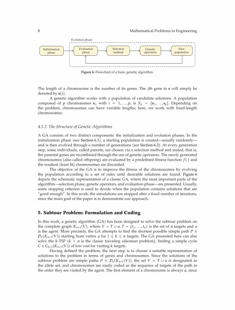
4.1.2. The Structure of Genetic Algorithms

A GA consists of two distinct components: the initialization and evolution phases. In theinitialization phase (see Section 6.1), a starting population is created—usually randomly—and is then evolved through a number of generations (see Section 6.2). At every generationstep, some individuals, called parents, are chosen via a selection method and mated, that is,the parental genes are recombined through the use of genetic operators. The newly generatedchromosomes (also called offspring) are evaluated by a predefined fitness function f(·) andthe weakest (least fit) chromosomes are discarded.

The objective of the GA is to improve the fitness of the chromosomes by evolvingthe population according to a set of rules until desirable solutions are found. Figure 6depicts the schematic representation of a classic GA, where the most important parts of thealgorithm—selection phase, genetic operators, and evaluation phase—are presented. Usually,some stopping criterion is used to decide when the population contains solutions that are“good enough”. In this work, the simulations are stopped after a fixed number of iterations,since the main goal of the paper is to demonstrate our approach.

5. Subtour Problem: Formulation and Coding

In this work, a genetic algorithm (GA) has been designed to solve the subtour problem onthe complete graph Kn+1(V ), where V = T ∪ a, T = {t1, . . . , tn} is the set of n targets and ais the agent. More precisely, the GA attempts to find the shortest possible simple path P ∈Pk(Kn+1(V )) starting from vertex a for 1 ≤ k ≤ n targets. The GA presented here can alsosolve the k-TSP (k = n is the classic traveling salesman problem), finding a simple cycleC ∈ Ck+1(Kn+1(V )) of low cost for visiting k targets.

Having defined the problem, the next step is to choose a suitable representation ofsolutions to the problem in terms of genes and chromosomes. Since the solutions of thesubtour problem are simple paths P ∈ Pk(Kn+1(V )), the set V = T ∪ a is designated asthe allele set, and chromosomes are easily coded as the sequence of targets of the path inthe order they are visited by the agent. The first element of a chromosome is always a, since


t1

a

t4

t2

t5t3

(a) Targets and agents

v1

v6

v4

v2

v5v3

(b) Path in P4(K6(V ))

a t1 t3 t5 t2

(c) Chromosome

Figure 7: Order-based representation: the chromosome (possible solution) is coded as the sequence ofvisited targets. In (a), the set of targets T = {t1, . . . , t5} and the agent a are shown. In (b), a path visiting 4targets (P ∈ P4(K6(V ))) is illustrated on the vertex set V = T∪a. The associated chromosome is representedas the sequence of the visited targets, with a = v6, thus s = (a, t1, t3, t5, t2) (see (c)).

the starting point of the agent is r(a). Therefore, a generic chromosome/path is representedas s = (x1, x2, . . . , xk), with x1 = a and xi ∈ T . An additional constraint on the structureof the chromosome is imposed by the simplicity of the path (every target should be visitedonly once) therefore; the same gene must not appear in the chromosome more than once. Thecoding for the k-TSP is similar.

The total cost c(·) of a chromosome/path s = (x1, . . . , xk) is the sum of the weights ofits edges (in other words the distance between targets)

c(s) =k∑

i=2

‖r(xi) − r(xi−1)‖, (5.1)

while its fitness value is defined as 1/c(s) (the lower the cost, the higher the fitness and viceversa).

The above representation is called order based, and the fitness of an individualdepends on the order of the genes in the chromosome, as opposed to the traditionalrepresentation where the order is not important [38]. As an example, consider agent a and thecomplete graph Km(V ) generated by the augmented vertex set V (with |V | = m). A genericpath P = (V1, E1) ∈ Pk(Km(V )), with V1 = {x1, . . . , xk+1}, E1 = {(x1, x2), . . . , (xk, xk+1)} andx1 = a, is coded in the chromosome s = (x1, . . . , xk+1) (see Figure 7).

A class of genetic operators have been developed for the variants of the k-TSP [38, 51]and some of these are described in the following (see Section 6.3).

6. Implementation of the Genetic Algorithm

In this section, a fixed-length chromosome implementation of the genetic algorithm (GA)for solving the subtour problem is described. The two main components of the GA are theinitialization and the evolution phases.

6.1. Initialization Phase

The starting population of chromosomes determines not only the starting point for theevolutionary search, but also the effectiveness of the algorithm. One of the problems usingGA is that the algorithm could prematurely converge to local minima instead of exploring


more of the search space. This occurs when the population quickly reaches a state wherethe genetic operators can no longer produce offsprings outperforming their parents [52]. It isimportant to point out that the size of the starting population also influences the performanceof the algorithm, since a population too small can lead to premature convergence, while a bigone could bring the computation to a crawl.

For the combinatorial problems of interest, a hard constraint is enforced: every gene(representing a target) must only be present once in every chromosome.

6.2. Genetic Evolution Phase

After the initialization phase, the initial population is evolved. The chromosomes of the ithgeneration are combined, mutated and improved through genetic operators (see Section 6.3)to create new chromosomes (the offsprings). These are then evaluated by the fitness function:the weakest (least fit) solutions are discarded while the good ones are kept for the i + 1thgeneration. The evolution phase consists of three main parts: selection of parents, applicationof genetic operators and creation of a new population by evaluation of the offsprings. Ifduring the selection phase two identical parents are chosen, the recombination processmay result in duplication of chromosomes which may decrease the heterogeneity of thepopulation. This could lead to the quick reduction of the coverage of the search space andthe consequently fast and irreversible convergence towards local minima far away from theoptimal solution.

This premature convergence is not desirable and different methods have been devisedto get around this problem. For example, in the random offspring generation technique[51] the genetic operators are applied only if the genetic materials of the parents aredifferent, otherwise at least one of the offsprings is randomly generated. Other, even moredrastic, solutions have been proposed. In [53] the social disasters technique is applied tothe TSP in order to maintain the genetic diversity of the population. This method checks theheterogeneity of the population and, if necessary, replaces a number of selected chromosomesby randomly generated ones.

To counter the effect of premature convergence, we decided to maintain heterogeneityof the populations by introducing what we call a singular mating pool. This pool is created ateach generation step from the population by removing all duplicates. Consequently, if thepopulation has n individuals, the singular mating pool is always composed of nSMP ≤ nsolutions. With this method, the probability of mating identical chromosomes is reduced.However, note that an individual can be selected and mated more than once. The singularmating pool does not preclude the duplication of individuals, it only reduces its frequency,resulting in a higher diversity of the solutions and avoiding premature convergence.

For the selection phase the Tournament Selection method [38, 54] is adopted. Asubset of the nSMP chromosomes is randomly chosen from the Singular Mating Pool andthe best chromosome is selected for the so-called mating pool. This process is repeated untila predefined number of individuals, ntournament, is reached (in our simulations ntournament =nSMP/2).

From the mating pool two parents are randomly selected, and to these, the geneticoperators are applied with some predefined probability (see Section 6.3). This process isrepeated until nnew offsprings have been generated. These new chromosomes are then addedto the singular mating pool (of size nSMP), returning a new temporary population of sizentemp = nSMP + nnew. In this work, nnew is chosen such that ntemp = 1.5n. Since the requirednumber of chromosomes in a population is n, the ntemp − n = n/2 weakest individuals


Parent B

Parent ApDXO pmutation p2−opt

Probabilities of application are checked

Offspring B

Offspring A

Crossoveroperator

Mutationoperator

Local 2-optboosting

nnewntempU

Removal of weakestchromosomes

n

Populationn

Singular mating poolnSMP Tournament

selection ntournament

Matingpool

Geneticoperators

Figure 8: Genetic algorithm schema with the singular mating pool technique and the application of thegenetic operators. Note that given two parents, first the crossover operator is applied, followed by themutation. The offsprings are then “boosted” with the 2-opt method.

(the ones with the highest cost c, c.f. (5.1)) are discarded. The adopted schema is shownin Figure 8.

6.3. Genetic Operators

Genetic operators combine existing solutions into new ones (crossover) or introduce randomvariations (mutation) to maintain genetic diversity. These operators are applied in a fixedorder (shown in Figure 8) with a priori assigned probabilities. In addition to these operators,the heuristic 2-opt method to directly improve the fitness of the offsprings is used (seeSection 6.3.4).

Different crossover typologies have been developed for solving the classic TSP,including the partially matched crossover, order crossover, and cycle crossover operators[38]. These operators are all based on the constraint that TSP solutions include allthe targets. Since this is not the case for the Subtour Problem, these operators cannotbe directly applied. To overcome these limitations, we modified the classic operatorsaccording to the new problem constraints. In particular, we decided to use a standardgenes recombination mechanism, while changing the rules for keeping the feasibility of thesolutions.

6.3.1. Single Cutting-Point Crossover

With the single cutting-point crossover (applied with probability pXO), both parents arehalved at the same gene, the cutting point (see Figure 9).


Cutting point

t1 t2 t3 t4 t5

t6 t7 t8 t9 t0

t1 t2 t8 t9 t0

t6 t7 t3 t4 t5

Figure 9: Single cutting-point crossover: parents are halved at the same gene.

Cutting point

Cutting point

t0 t1 t2 t3 t4 t5

t6 t7 t8 t9 t10 t11

t0 t1 t6 t7 t8 t9

t9 t10 t2 t3 t4 t5

Figure 10: Double cutting-point crossover: parents are cut at two different genes.

The cutting point is chosen either randomly or to break the longest edge in the parents(with plong-cut probability). Once the parents have been halved, two offsprings are createdcombining the first (second) half of the first parent with the second (first) half of the secondparent, respectively. Care is taken to avoid duplication of genes (as every target should onlybe visited once) and the length of the chromosomes is kept constant. See Appendix A for anillustrative example.

6.3.2. Double Cutting-Point Crossover

The double cutting-point crossover operator cuts the parents at two different genes (seeFigure 10), with probability pDXO. The locations of the cutting points are chosen eitherrandomly or to cut the longest edge in the parents (with plong-cut probability). The latterintroduces an improvement over the single cutting-point operator, where only one parentwas cut along its longest edge and this point was also used for the other parent. An importantconsequence of having two different cutting points is that the halves will in general havedifferent number of genes. A simple recombination would thus lead to two offsprings withdifferent lengths. The technique to maintain the original size of the chromosomes (which isnecessary for producing feasible solutions) is described in Appendix B.

6.3.3. Mutation Operator

After the application of the crossover operator, the mutation operator is applied to thenew chromosomes with pmutation. The mutation operator generates a new offspring byrandomly swapping genes (Figure 11) and/or randomly changing a gene to another onethat is not already present in the chromosome (Figure 12). Note that with the simple TSP,this second type of mutation would not be possible, because there a chromosome alreadycontains all possible genes. The probability of the mutation is a parameter of the geneticalgorithm.


t1

a t4

t2

t5t3

(a) Before gene swapping

t1

a t4

t2

t5t3

(b) After gene swapping

Figure 11: Given a chromosome s1 = (a, t1, t4, t3, t2, t5) (shown in (a)), (b) shows the chromosome s2 =(a, t1, t2, t3, t4, t5) resulting after genes t4 and t2 are swapped.

t1

at4

t3

t2

(a) Before gene mutation

t1

at4

t3

t2

(b) After gene mutation

Figure 12: Given a chromosome s1 = (a, t1, t2, t3) (shown in (a)), (b) shows the chromosome s2 =(a, t1, t4, t3) after t2 mutated into t4.

6.3.4. Improving Offsprings

A common approach for improving the TSP solutions is the coupling of the genetic algorithmwith a heuristic boosting technique. The local search method adopted here is the 2-optmethod [55–57] that replaces solutions with better ones from their “neighborhood”.

Let us consider a set T of n targets and the corresponding complete and weightedgraph Kn+1(V ) (V = T ∪ a with a being the agent). Let us consider a subtour P ∈ Pk(Kn+1),with 1 ≤ k ≤ n, coded in the chromosome s = (x1, . . . , xk). The 2-opt method determineswhether the inequality

w(xi, xi+1) +w(xj , xj+1

)> w(xi, xj

)+w(xi+1, xj+1

), (6.1)

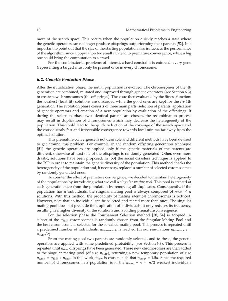
between the four vertices xi, xi+1, xj and xj+1 of P holds, in which case edges (xi, xi+1)and (xj , xj+1) are replaced with the edges (xi, xj) and (xi+1, xj+1), respectively. This methodprovides a shorter path without intersecting edges. Consequently, the order of genes in thechromosome changes [58] (see Figure 13). This operator is applied with p2-opt probability.

7. Results

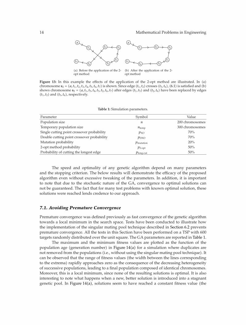
A large number of simulations have been performed to test the performance of theimplemented genetic algorithm. In order to evaluate the proposed method and providestatistically significant results, different problem configurations have been considered,including randomly generated problems and problems with known optimal solutions. Unlessotherwise specified, the tests described here are all run for 250 generations with a populationsize of 200 chromosomes. The crossover, mutation, and boosting (2-opt) operators are appliedwith a pXO = pDXO = 70%, pmutation = 20%, and p2-opt = 50% probability, respectively. Table 1summarizes the parameters and their default values adopted for the simulations.


a

t1 t5 t4

t3t2t6

t7

(a) Before the application of the 2-opt method

a

t1 t5 t4

t3t2t6

t7

(b) After the application of the 2-opt method

Figure 13: In this example the effects of the application of the 2-opt method are illustrated. In (a)chromosome s2 = (a, t1, t2, t3, t4, t5, t6, t7) is shown. Since edge (t1, t2) crosses (t5, t6), (6.1) is satisfied and (b)shows chromosome s2 = (a, t1, t5, t4, t3, t2, t6, t7) after edges (t1, t5) and (t2, t6) have been replaced by edges(t1, t2) and (t5, t6), respectively.

Table 1: Simulation parameters.

Parameter Symbol ValuePopulation size n 200 chromosomesTemporary population size ntemp 300 chromosomesSingle cutting point crossover probability pXO 70%Double cutting point crossover probability pDXO 70%Mutation probability pmutation 20%2-opt method probability p2-opt 50%Probability of cutting the longest edge plong-cut 50%

The speed and optimality of any genetic algorithm depend on many parametersand the stopping criterion. The below results will demonstrate the efficacy of the proposedalgorithm even without excessive tweaking of the parameters. In addition, it is importantto note that due to the stochastic nature of the GA, convergence to optimal solutions cannot be guaranteed. The fact that for many test problems with known optimal solution, thesesolutions were reached lends credence to our approach.

7.1. Avoiding Premature Convergence

Premature convergence was defined previously as fast convergence of the genetic algorithmtowards a local minimum in the search space. Tests have been conducted to illustrate howthe implementation of the singular mating pool technique described in Section 6.2 preventspremature convergence. All the tests in this Section have been performed on a TSP with 600targets randomly distributed over the unit square. The GA parameters are reported in Table 1.

The maximum and the minimum fitness values are plotted as the function of thepopulation age (generation number) in Figure 14(a) for a simulation where duplicates arenot removed from the populations (i.e., without using the singular mating pool technique). Itcan be observed that the range of fitness values (the width between the lines correspondingto the extrema) rapidly approaches zero as the consequence of the decreasing heterogeneityof successive populations, leading to a final population composed of identical chromosomes.Moreover, this is a local minimum, since none of the resulting solutions is optimal. It is alsointeresting to note what happens when a new, better solution is introduced into a stagnantgenetic pool. In Figure 14(a), solutions seem to have reached a constant fitness value (the


0

0.5

1Fi

tnes

sva

lues

0 50 100 150 200

Number of generations

Maximum fitness valuesMinimum fitness valuesOptimal fitness value

(a) The singular mating pool is not used

0

0.5

1

Fitn

ess

valu

es

0 50 100 150 200


Maximum fitness valuesMinimum fitness valuesOptimal fitness value

(b) The singular mating pool is used

Figure 14: (a) Simulation without using the singular mating pool. The duplicated chromosomes leadto premature convergence. (b) Simulation with the singular mating pool technique. With duplicatechromosomes removed from the populations, the diversity of solutions is maintained.

plateau around the 80th generation), when a better chromosome randomly appears in thepopulation around the 120th generation.

Since during the evolution the duplicates of this chromosome are not discarded (itsfitness value is better than those of the other solutions), in a small number of generationsthey replicate and replace all other individuals.

Figure 14(b) shows the extremal values of fitness in a simulation where the duplicatesare constantly removed from the mating pool; that is, where the singular mating pool methodis used. As a result of this strategy the diversity of the populations is maintained with anincreased coverage of the search space. This makes it more likely for the algorithm to reach anear-optimal solution (in this case, the optimal result is reached).

To characterize the heterogeneity/diversity of a population, a pairwise comparison ofchromosome edges can be used. Let us consider two chromosomes of length k, si, and sj ,with edge sets Ei and Ej , respectively (|Ei| = |Ej |). One possible measure of diversity can bedefined as

di,j = 1 −∣∣Ei ∩ Ej

∣∣

|Ei|. (7.1)

This edge diversity quantifies how much two chromosomes differ. The exact locationsof identical edges do not influence this diversity measure. The edge diversity of the entirepopulation Sp is the averaged edge diversities for all pairs

DSp =1

n(n − 1)

p−1∑

i=1

p∑

j=i+1

di,j . (7.2)

Clearly, 0 ≤ DSp ≤ 1. We also introduce a “Boolean” diversity. The diversity of twochromosomes are equal if and only if they have identical edges. The Boolean diversity for


0

20

40A

vera

geed

ged

iver

sity

(%)

0 10 20 30 40 50 60 70 80 90 100


Without singular mating poolWith singular mating pool

(a) Edge diversity

0

20

40

60

80

100

Ave

rage

div

ersi

ty(%

)

0 50 100 150 200 250


Without singular mating poolWith singular mating pool

(b) Boolean diversity

Figure 15: How the application of the singular mating pool technique affects the edge (a) and boolean (b)diversity (%) of the population.

population Sp is defined as

BSp =p−1∑

i=1

p∑

j=i+1

⎧⎪⎨

⎪⎩

0 if di,j = 0,

1 if di,j /= 0.(7.3)

Figure 15 shows the average edge and boolean diversity at every generation step forthe simulations used for Figure 14 (with or without the use of the singular mating pooltechnique).

The decrease of the edge diversity can be explained by the reduction of the coverage ofthe search space: many costly edges are discarded early in the evolution and only consideredagain during the search process with low probability. This is why at later generations manysolutions differ only by few edges, but still the population maintains its heterogeneity (asshown in Figure 15(b)).

In conclusion, to avoid premature convergence it is important to ensure that theevolving population contains a variety of chromosomes (representing different strategies forthe agent to reach a set of targets). In our work on distributed planning (published in thesequel), the availability of these different strategies will have special significance.

7.2. Influence of the 2-opt Method on the Performance of Genetic Operators

To evaluate the performance of the different genetic operators and the 2-opt method, varioustests have been performed. A target configuration for n = 100 targets randomly anduniformly distributed over the unit square is generated. This configuration is kept fixed forall tests in this section to make comparisons meaningful. The 30-from-100 subtour problemis then solved with different combinations of the genetic operators, 100 times for eachcombination. The application probabilities of the operators are reported in Table 1. To assessthe influence of the various genetic operators, their performances are directly compared and


Table 2: Simulation cases to test efficiency of different genetic operators. The 2-opt method is not applied.

Crossover type Mutation Mean fitness Variance of fitnessDouble point Applied 1 1Single point Applied 0.93 1.32Double point Not applied 0.92 1.47Single point Not applied 0.69 2.12

Table 3: Simulation cases to test efficiency of different genetic operators together with the 2-opt method.

Crossover type Mutation Mean fitness Variance of fitnessDouble point Applied 0.993 3.12Single point Applied 1 1Double point Not applied 0.994 2.62Single point Not applied 0.998 1.31

tested without the 2-opt method. The mean values and the variances of the distribution of thebest (highest) fitness values of the final populations are shown in Table 2.

Since the optimal solution is not known, the mean fitness values and the variances offitness are normalized by the best result (the highest for the fitness values and the lowestfor the variances of fitness). The comparison of the quantities in Table 2 shows that thecombined application of the double cutting-point crossover and the mutation operator yieldsthe maximum fitness value and the minimum variance of the solutions. On the other hand,the worst solutions are obtained with the standalone application of the single cutting pointcrossover operator. These results not only demonstrate the improvement introduced by thedouble cutting point crossover, but also clearly highlight the importance of the mutationoperator.

With the application of the 2-opt method, the results change, as shown in Table 3.In this case, the performance of the single cutting-point crossover operator coupled

with mutations is the best. It would be tempting to conclude that this configuration of thegenetic operators is the best; however, in the next section it is demonstrated that the speedof convergence for this configuration of operators is significantly worse than for the doublecutting-point crossover/mutation combo (here, this fact is hidden as the genetic algorithm isrun for a fixed number of generations).

7.3. Speed of Convergence and Genetic Operators

The results of the previous section clearly demonstrate the efficiency of coupling the geneticoperators with the 2-opt method. The most important improvement introduced by the 2-optmethod is in the speed of convergence that is here intended as the number of generation thealgorithm requires for converging (it is not related to time). In fact, because of its capabilityof detecting new local minima at each generation step, the application of the 2-opt methodtogether with the double cutting-point crossover and the mutation operators helps the GA toconverge faster than without [56]. To quantify the speed of convergence with various geneticoperators and the 2-opt method, the required number of generations for the convergence ofthe genetic algorithm is calculated. To facilitate this test, a 100-target TSP with known exactsolution was solved (KroA-100 TSP [59], with optimal path-length of 21282). For different


Table 4: GA solution of the KroA100 problem [59]. The 2-opt method is always applied and the numberof generations necessary for the convergence of the full population within 1% of the optimal solution isevaluated with respect to different configurations of genetic operators.

Crossover type Mutation Number of generations VarianceDouble Applied 7.7 1Double Not applied 8.7 1.14Single Applied 14.3 1.86Single Not applied 15.8 1.93

Table 5: Comparison of the proposed method with benchmarked solutions of the traveling salesmanproblem. Results are averaged over 100 simulations. Rounded distances are used.

Problem TSPLIB Number of targets Optimal tour Genetic algorithm error

Length Minimum Mean Maximum Std

Berlin52 52 7542 0% 0% 0% 0Eil76 76 538 0% 0.02% 1.4% 0.8KroA100 100 21282 0% 0% 0% 0lin105 105 14379 0% 0% 0% 0ch130 130 6110 0% 0.2% 0.9% 15.9a280 280 2579 0% 0.2% 1% 8.5pcb442 442 50778 0.3% 0.9% 1.5% 148.6att532 532 86729 0.4% 1.1% 2% 340.07

combinations of the genetic operators, Table 4 reports the number of generations (and itsvariance) necessary to reach a solution within 1% of the optimal length. For each case, 500simulations have been performed and the variance of the final results is normalized withrespect to the minimum obtained value. From these results, we conclude that the GA withdouble cutting-point crossover coupled with the mutation operator needs the least numberof generations to reach a near-optimal solution (for this example, the local boosting techniqueyielded a 25-fold increase in computational speed to reach populations with the same fitness).Results on the runtime performance for the method were published in [60].

7.4. TSP Tests

Since the TSP is a limiting case of the subtour problem (one agent visiting all the targets,that is, m = 1, k = n, with the restriction on returning to the starting position) the proposedalgorithm can also be used to solve this classic problem.

The algorithm has been tested with different TSPs from the well-known TSPLIB95library [59]. This library includes different target configurations for the TSP and many relatedproblems (Hamiltonian cycle problem, sequential ordering problem, etc.) together with theirexact solutions. We note that the TSPs in the TSPLIB95 library are solved with a cost functionbased on rounded distances between targets. In order to have meaningful comparisons withthe TSPLIB95 problems, our cost function was modified to round off distances.

For every TSPLIB95 instances considered here, 100 simulations have been performedand the operators are applied with the probabilities reported in Table 1. The results are shownin Table 5 and demonstrate the suitability of our approach.


0

2500

5000

Yco

ord

inat

e0 2500 5000 7500

X coordinate

(a) att532 problem: optimal solution

(b) Optimal solution (c) GA solution

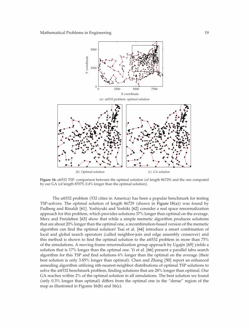
Figure 16: att532 TSP: comparison between the optimal solution (of length 86729) and the one computedby our GA (of length 87075, 0.4% longer than the optimal solution).

The att532 problem (532 cities in America) has been a popular benchmark for testingTSP-solvers. The optimal solution of length 86729 (shown in Figure 18(a)) was found byPadberg and Rinaldi [61]. Yoshiyuki and Yoshiki [62] consider a real space renormalizationapproach for this problem, which provides solutions 37% longer than optimal on the average.Merz and Freisleben [63] show that while a simple memetic algorithm produces solutionsthat are about 20% longer than the optimal one, a recombination-based version of the memeticalgorithm can find the optimal solution! Tsai et al. [64] introduce a smart combination oflocal and global search operators (called neighbor-join and edge assembly crossover) andthis method is shown to find the optimal solution to the att532 problem in more than 75%of the simulations. A moving-frame renormalization group approach by Ugajin [65] yields asolution that is 17% longer than the optimal one. Yi et al. [66] present a parallel tabu searchalgorithm for this TSP and find solutions 6% longer than the optimal on the average (theirbest solution is only 3.85% longer than optimal). Chen and Zhang [50] report an enhancedannealing algorithm utilizing nth-nearest-neighbor distributions of optimal TSP solutions tosolve the att532 benchmark problem, finding solutions that are 28% longer than optimal. OurGA reaches within 2% of the optimal solution in all simulations. The best solution we found(only 0.3% longer than optimal) differs from the optimal one in the “dense” region of themap as illustrated in Figures 16(b) and 16(c).


Table 6: Comparison of the proposed method with different TSPs solved using the CONCORDE algorithm.For each case, 100 simulations have been run. Rounded distances are used.

Number of targets Optimal tour Genetic algorithm error

Length Minimum Mean Maximum Std

600 1812 0.7% 1.3% 2.2% 5.6700 1946 0.9% 2% 2.8% 7.6800 2087 1.3% 2.1% 2.8% 9.11000 2297 4.2% 5.3% 6.7% 11.1

Table 7: Efficacy of the singular mating pool. Results are averaged over 100 simulations. Consideredproblem: TSP of 600 cities with optimal tour length equal to 1812.

Singular mating poolGenetic algorithm error

Minimum Mean Maximum Std

Applied 0.5% 1.3% 2.3% 7.01

Not applied 1.1% 2.1% 3.6% 7.8

Optimal TSP solutions for targets uniformly distributed over the unit square wereobtained using CONCORDE [67] (also using rounded distances). Table 6 summarizes theresults.

Once again, the GA-based approach seems to perform well. The sudden increase inthe errors for the 1000-target problem can be attributed to the relatively low size of thepopulations and to the fact that the number of the generations (250) used in these simulationsis fixed (note that the objective of these tests was not to reach the best possible solutions).

Finally, to quantify the influence of the singular mating pool technique, Table 7 showsthe different results obtained with or without its application. These simulations illustrate thatavoiding the replication of the individuals through the application of the singular matingpool (slightly) improves the solutions. Note that the main purpose of the Singular MatingPool is to maintain diversity of possible subtours. This has special significance for buildingnear-optimal multiagent plans.

The results of this section strengthen our claim that the implemented genetic algorithmis successful in finding near-optimal solutions for this type of combinatorial problems.

7.5. Subtour Tests

The genetic planner has also been statistically tested in order to demonstrate its capabilityto generate near-optimal subtours. To provide reliable averages, for a given configuration100 simulations have been performed. All the subtour tests have been conducted on theunit square with a given target configuration and using the cost function (2.4). The doublecutting-point crossover, the mutation operator, and the 2-opt method have been used (withthe probabilities reported in Table 1).

In order to evaluate the optimality of the subtours generated by our genetic algorithm,a comparison with known optimal solutions is needed. To our knowledge, no benchmarksolutions exist for the subtour problem, so we introduced test cases with regular and randompoint configurations on the unit square to evaluate the algorithm.


0

0.5

1

Yco

ord

inat

e

0 0.5 1

X coordinate

Figure 17: Example of a subtour problem generated by a 7 × 7 grid (circles), with 9 more added targets(squares).

Table 8: Comparison between exact and GA solutions for different Subtour Problems based on 100simulations.

n lNumber of targets Subtour Optimal tour Genetic algorithm error

n2 + l (l + 2)-from-(n2 + l) Length Minimum Mean Maximum Std

7 9 58 11-from-58 0.236 0% 0% 0% 0

11 15 136 17-from-136 0.141 0% 0.2% 12.5% 0.002

21 48 489 50-from-489 0.07 0% 656.6% 2883.4% 0.43

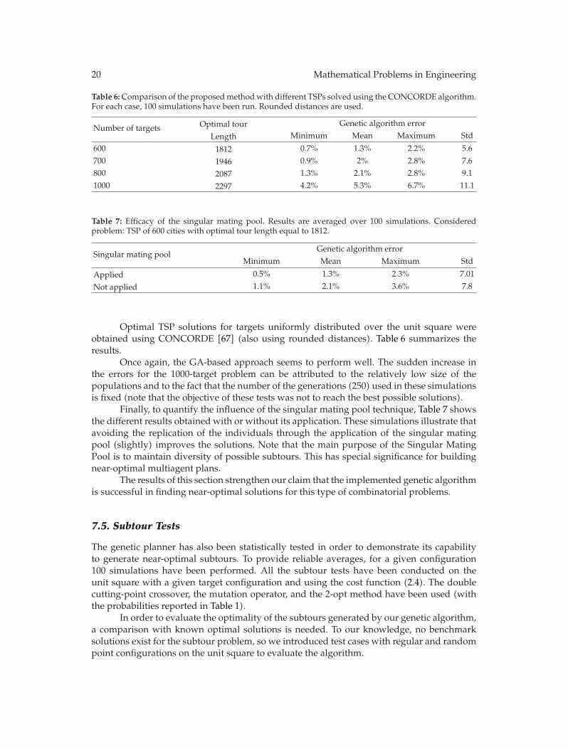
The first set of tests have been conducted by generating maps of targets with a trivialunique optimal solution. In these tests, n2 targets were selected with constant spacing of 1/non the unit square (a uniform grid) with l extra points added between two points of the grid,following vertical, horizontal or diagonal directions. Figure 17 shows an example depictingthe optimal 11-from-58 solution (n = 7, l = 9).

Different problems have been generated and the results are shown in Table 8.We note that the proposed method converges to the optimal solution in almost all

the performed simulations. In few cases (the results of the 50-from-489 subtour), however,only very costly solutions (with high length) are found. This can be attributed to the slowconvergence of the stochastic optimization process. In fact, all the reported tests are run with afixed number of 250 generations which is in some cases not enough to ensure the convergenceof the GA to an optimal (or near-optimal) solution.

To elucidate this point, Figure 18(a) shows the percentage of simulations reaching theoptimal solution of the 50-from-489 problem as the function of population age (numberof generations), while Figure 18(b) shows the distribution of subtour lengths after 250generations. Note that only few of them are very costly solutions.

The speed of convergence of the algorithm strongly depends on the GA parameters.In particular, it is influenced by the application of the 2-opt method.

To provide numerical evidence for this claim, 100 simulations have been run on the 17-from-133 targets problem shown in Figure 19 with different application probabilities of the 2-opt method. Note that in this case, the l points are added between more than two neighboringpoints.


0

20

40

60

80

100

Sim

ulat

ions

tore

ach

ane

ar-o

ptim

also

luti

on(%

)

0 250 500 1000 1500 2000


(a) Speed of convergence

0

5

10

15

20

25

30

Sim

ulat

ions

(%)

0 1 10 20 30

Subtour length

(b) Distributions of subtour lengths after 250 gener-ations

Figure 18: The convergence of the 50-from-489 Subtour Problem is shown. Subtour lengths are normalizedwith the optimal one (length = 0.0707). In (a) the speed of converge is shown. Note that the last simulationconverges after 2045 generations. (b) Shows the distribution of the subtour lengths after 250 generations,considering 100 simulations.

0

0.5

1

Yco

ord

inat

e

0 0.5 1

X coordinate

Figure 19: Example of a subtour problem generated by a grid of 112 targets (circles), with 12 more addedpoints (squares).

Table 9: Convergence results for the 17-from-133 problem with different 2-opt method probabilities.

2-opt probability Simulations converged after 250generations

Number of generations for fullconvergence

0.05 15% 431480.2 34% 121800.5 84% 728

1 94% 1233

Results are reported in Table 9, while Figure 20 shows the convergence speeds fordifferent values of the 2-opt application probability.

In general, the frequent use of the 2-opt method restricts the random wandering ofthe genetic algorithm over the search space, thereby severely restricting the set of reachablesolutions. If the 2-opt method is only applied with a given probability, much like the other


0

20

40

60

80

100

Sim

ulat

ions

tore

ach

ane

ar-o

ptim

also

luti

on(%

)0 250 500 750 1000


10.5

0.2

0.05

Figure 20: Convergence for the GA solution of a 17-from-133 subtour problem with different applicationprobabilities of the 2-opt method.

Table 10: Comparison between exact and GA solutions for different subtour problems based on 100simulations.

Subtour Optimal length GA solution length Mean error

7-from-30 0.71 0.72 1.4%

6-from-30 0.628 0.63 0.3%

6-from-40 0.53 0.56 5.6%

5-from-50 0.446 0.447 0.4%

operators, the results greatly improve and the number of necessary generations are stronglyreduced.

Note also (see Table 9) that if the 2-opt method is always applied, the number ofgenerations needed for full convergence can be very high.

Another set of tests have been devised to compare GA subtour solutions to exactones in random configurations of targets in the unit square. To find the exact solutions forthese tests, the simplest brute force approach (exhaustive evaluation of combinations) wasused. Figure 21 shows an optimal 7-from-30 subtour with specified starting point (the depot)and the solution found by the GA. Table 10 summarizes the results for different subtourproblems.

Figure 22 shows a sample subtour for a problem, where the total number of targets isn = 100 and the shortest path is sought connecting any k = 20 targets (a no depot problem).

As previously described, the Subtour solutions can be used as a starting set of solutionsfor solving the more challenging multiagent planning problem. In Figure 23, few preliminaryexamples are shown from our work on the multiagent planning problem.

8. Conclusions

This paper describes a genetic goal planner for generating a near-optimal strategy, a subtour,for visiting a subset of known targets/goals. The importance of this work is to provide theability to a single agent to plan a strategy—a subtour—by organizing a sequence of targetsautonomously. This planning capability is a starting step toward a multiagent planning


0

0.5

1

Yco

ord

inat

e

a

0 0.5 1

X coordinate

Exact solutionGA subtour

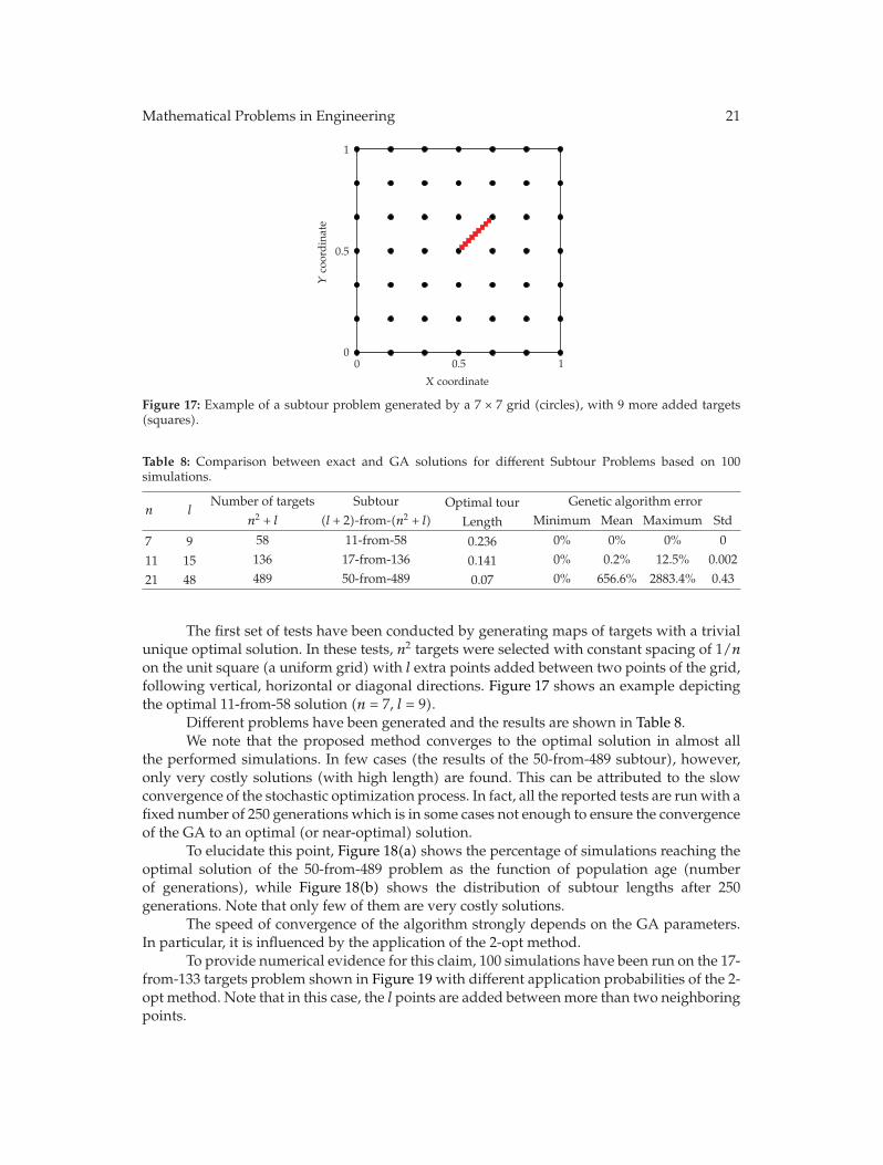
Figure 21: Comparison between the exact 6-from-40 subtour (length = 0.53) and the GA solution (length =0.58). The fixed starting point (depot) is a.

0

0.5

1

Yco

ord

inat

e

0 0.5 1

X coordinate

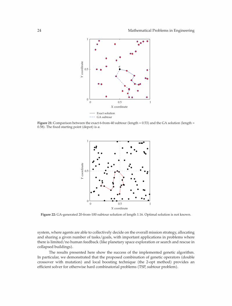
Figure 22: GA-generated 20-from-100 subtour solution of length 1.16. Optimal solution is not known.

system, where agents are able to collectively decide on the overall mission strategy, allocatingand sharing a given number of tasks/goals, with important applications in problems wherethere is limited/no human feedback (like planetary space exploration or search and rescue incollapsed buildings).

The results presented here show the success of the implemented genetic algorithm.In particular, we demonstrated that the proposed combination of genetic operators (doublecrossover with mutation) and local boosting technique (the 2-opt method) provides anefficient solver for otherwise hard combinatorial problems (TSP, subtour problem).


0

2

4

6

8

10

12

14×103

Yco

ord

inat

e

0 5 10 15 20×103

X coordinate

(a) 76 cities and 5 agents

0

1

2×103

Yco

ord

inat

e

0 2 4×103

X coordinate

(b) 100 cities and 5 agents

Figure 23: MAPP examples.

Cutting point

s1

s2

1 2 3 4 5 6 7 8

3 9 8 4 0 5 6 2

(a) Parents s1 and s2 are cut at the samepoint

s1

s2

s3

s4

1 2 3 4 5 6 7 8

3 9 8 4 0 5 6 2

1 2 3 4 0 5 6 2

3 9 8 4 5 6 7 8

(b) Two new temporary solutions, s3 and s4, are generated, but some replications can occur

Figure 24: Single cutting-point crossover. For clearness, only the indexes of the targets are reported andagent a is not shown.

Appendices

A. Single Cutting-Point Crossover

With the single cutting-point crossover operator, parents are halved at the same gene. Thecutting point is chosen either randomly or to break the longest edge in the parents (theprobability of which one of the two methods is applied is specified a priori).

Consider two parents, s1 = (a, t1, t2, t3, t4, t5, t6, t7, t8) and s2 = (a, t3, t9, t8, t4, t0, t5, t6, t2).Since the first gene in all the chromosomes is always a, for clarity we only show the operationsof the target genes. Figure 24(a) shows the two parents both being cut at the fourth gene.

Once the parent chromosomes are divided, the two offsprings s3 and s4 are createdby combining the first (second) half of s1 with the second (first) half of s2, respectively.This operator is designed to preserve the length of the chromosomes. However, as shownin Figure 24(b), a simple recombination of the halves of the parents could result in unfeasiblesolutions, since some targets could appear twice in the same chromosome (e.g., target t2 in s3

appears twice, so does target t8 in s4).


s4

s1

s3

3 9 8 4 5 6 7 8

1 2 3 4 5 6 7 8

1 2 3 4 0 5 6 2

3 9 3 4 5 6 7 8

1 2 3 4 5 6 7 8

1 2 3 4 0 5 6 8

s4

s1

s3

Figure 25: Single cutting-point crossover: new feasible solutions. For clarity, only the indices of the targetsare reported and agent a is not considered.

Cutting point

Cutting point

s1

s2

1 2 3 4 5 6 7 8

3 7 5 4 0 1 6 9

(a) Double cutting-point crossover: parentsare cut at two different points

s3

s4

s2

s1

3 7 5 4 0 1 6 9

1 2 3 4 5 6 7 8

1 2 1 6 9

3 7 5 4 0 3 4 5 6 7 8

(b) Double cutting-point crossover: halves have differentsize

Figure 26: Double cutting-point crossover: a simple recombination is not possible, since the new offspringss3 and s4 can have different lengths. For clearness, only the indexes of the targets are reported and agent ais not shown.

To restore the feasibility of the solutions, the replicated genes in the offsprings must bereplaced by ones not already present in these chromosomes. To achieve this, the followingreplacement method has been devised. Without loss of generality, let us suppose that inboth chromosomes s3 and s4 only genes that originate from parent s2 need to be replaced.Therefore, when a gene is replaced, it is replaced by the corresponding gene in parent s1.This method is applied iteratively, until two feasible solutions (without gene repetitions) areobtained.

In the example shown in Figure 25, genes are substituted as follows. At first, sinces3(8) = s3(2) = 2, gene s3(8) is replaced by the corresponding gene s1(8) = 8. At the samestep, since s4(3) = s4(8) = 8, gene s4(3) is replaced by the corresponding gene s1(3) = 3.At the end of this first iteration, the new offspring s4 is still unfeasible (s4(1) = s4(3) = 3).Therefore, a new step is performed and s4(1) is replaced by s1(1) = 1. Note that only thegenes that came from parent s2 have been replaced.

This way, the substitutions are executed without introducing new targets, and thus,the genetic material of the parents is preserved.

B. Double Cutting-Point Crossover

With the double cutting point crossover operator the cutting points of the parents canbe different (see Figure 26(a)). The cutting points can be selected in two different ways,


s1

s3

s4

1 2

3 4 5 6 7 8

1 2 3 4 5 6 7 8

Figure 27: Double cutting-point crossover: at first, the offsprings s3 and s4 are filled with the genes of theparent s1. For clearness, a is not considered, since it is always at the beginning of the chromosomes.

Table 11: The first (second) half of the chromosome s3 (s4) is filled with the first (second) half of parent s1.

s1 = (x1, . . . , xi, xi+1, . . . , xk)

⇓s3 = (x1, . . . , xi, still empty)

s4 = (still empty xi+1, . . . , xk)

Table 12: Parent s2 is cut at gene j and the temporary chromosome s2 is derided from switching the halvesof s2.

s2 = (x1, . . . , xj , xj+1, . . . , xk)

⇓s2 = (xj+1, . . . , xk, x1, . . . , xj)

depending on preassigned probabilities plong-cut: they are chosen either randomly or tocut the longest edge in the parents. An important consequence of having two differentcutting points is that the halves of the parents may have a different number of genes. Thus,a simple swapping recombination would result in offsprings with different lengths (seeFigure 26(b)).

Since the length of the chromosomes is fixed (the number of targets in the subtour isgiven) to obtain feasible solutions, the offsprings are filled with the following ad hoc method.Consider two parents, s1 and s2, and their offsprings s3 and s4. Suppose that parent s1 is cut atthe ith gene, while parent s2 is cut at the jth gene. In the implemented method, at first, parents1 fills the offsprings s3 and s4 with its halves such that the first (second) half of the offsprings3 (s4) is the same as the first (second) half of s1 (see Figure 27 and Table 11).

Similarly to the example for the single cutting-point crossover, genes coming fromparent s1 will not be changed. For completing s3 and s4, only genes of parent s2 are used. Fora better explanation of the process for filling the remaining halves of the offsprings, let usintroduce the temporary chromosome s2; that is simply obtained by switching the halves ofs2 (obviously considering the cutting point j), as reported in Table 12.

The implemented method is based on both s2 and s2. At first, the second half of s3 isfilled using only the parent s2: starting from its first gene, and skipping the already presentgenes, offspring s3 is completed (see Figure 28). Then, offspring s4 is filled in the same waybut using the temporary chromosome s2.


s2

s3

s4

s2 1 6�� 9 3 7 5 4 0

1 9 3 4 5 6 7 8

1 2 3 7 5 4 0 6

3 7 5 4 0 1�� 6 9

Figure 28: Double cutting-point crossover: the second halves of the offsprings s3 and s4 are filled with theparent s2 and the temporary chromosome s2. As usual, the starting position is not considered, since it isalways at the beginning of the chromosomes.

Acknowledgments

The authors would like to thank the reviewers for their careful reading of the paper and theirconstructive criticism.

References

[1] E. T. Baumgartner, “In-situ exploration of Mars using rover systems,” in Proceedings of the AIAA Space2000 Conference, Long Beach, Calif, USA, 2000.

[2] S. Hayati, V. Volpe, P. Backes et al., “Rocky 7 rover: a Mars sciencecraft prototype,” in Proceedings ofthe IEEE International Conference on Robotics and Automation, vol. 3, pp. 2458–2464, Albuquerque, NM,USA, 1997.

[3] Mars Exploration Rover Missions, http://marsrovers.nasa.gov/home/.[4] Sojourner Rover Home Page, http://mpfwww.jpl.nasa.gov/rover/sojourner.html.[5] A. Birk and S. Carpin, “Rescue robotics—a crucial milestone on the road to autonomous systems,”

Advanced Robotics, vol. 20, no. 5, pp. 595–605, 2006.[6] S. Sariel and H. Akin, “A novel search strategy for autonomous search and rescue robots,” in RoboCup

2004: Robot Soccer World Cup VII, D. Nardi, M. Riedmiller, C. Sammut et al., Eds., vol. 3276/2005, pp.459–466, Springer, New York, NY, USA, 2005.

[7] G. Muscato, F. Russo, and D. Caltabiano, “Localization and self-calibration of a robot for volcanoexploration,” in Proceedings of the IEEE International Conference on Robotics and Automation, vol. 1, 2004.

[8] S. Carpin, J. Wang, M. Lewis, A. Birk, and A. Jacoff, “High fidelity tools for rescue robotics: resultsand perspectives,” in RoboCup 2005: Robot Soccer World Cup IX, vol. 4020 of Lecture Notes in ComputerScience, pp. 301–311, 2006.

[9] A. Jacoff, E. Messina, and J. Evans, Experiences in Deploying Test Arenas for Autonomous Mobile Robots,NIST Special, Gaithersburg, Md, USA, 2002.

[10] H. Kitano, “RoboCup-97: robot soccer world cup I,” Lectures Notes in Computer Science, vol. 1395 ofLecture Note in Artificial Intelligence, Springer, Berlin, Germany, 1998.

[11] T. Kalmar-Nagy, R. D’Andrea, and P. Ganguly, “Near-optimal dynamic trajectory generation andcontrol of an omnidirectional vehicle,” Robotics and Autonomous Systems, vol. 46, no. 1, pp. 47–64,2004.

[12] M. Ai-Chang, J. Bresina, L. Charest et al., “Mapgen: mixed-initiative planning and scheduling for themars exploration rover mission,” IEEE Intelligent Systems, vol. 19, no. 1, pp. 8–12, 2004.

[13] P. Maldague, A. Ko, D. Page, and T. Starbird, “APGEN: a multi-mission semi-automated planningtool,” in Proceedings of the 1st International NASA Workshop on Planning and Scheduling (AIAA ’97), A.press, Ed., 1997.


[14] N. Muscettola, P. P. Nayak, B. Pell, and B. C. Williams, “Remote agent: to boldly go where no AIsystem has gone before,” Artificial Intelligence, vol. 103, no. 1-2, pp. 5–47, 1998.

[15] K. H. Low, W. K. Leow, and M. H. Ang Jr., “A hybrid mobile robot architecture with integratedplanning and control,” in Proceedings of the International Conference on Autonomous Agents, pp. 219–226, ACM Press, Bologna, Italy, 2002.

[16] R. Sherwood, A. Mishkin, S. Chien et al., “An integrated planning and scheduling prototypefor automated Mars rover command generation,” Jet propulsion laboratory, california institute oftechnology, NASA, 2001.

[17] S. M. LaValle, Planning Algorithms, Cambridge University Press, Cambridge, UK, 2006.[18] A. Sipahioglu, A. Yazici, O. Parlaktuna, and U. Gurel, “Real-time tour construction for a mobile robot

in a dynamic environment,” Robotics and Autonomous Systems, vol. 56, no. 4, pp. 289–295, 2008.[19] P. Tompkins, A. Stentz, and D. Wettergreen, “Mission-level path planning and re-planning for rover

exploration,” Robotics and Autonomous Systems, vol. 54, no. 2, pp. 174–183, 2006.[20] J. Xiao, Z. Michalewicz, L. Zhang, and K. Trojanowski, “Adaptive evolutionary planner/navigator

for mobile robots,” IEEE Transactions on Evolutionary Computation, vol. 1, no. 1, pp. 18–28, 1997.[21] K. Savla, F. Bullo, and E. Frazzoli, “On traveling salesperson problems for dubins’ vehicle: stochastic

and dynamic environments,” in Proceedings of the 44th IEEE Conference on Decision and Control, and theEuropean Control Conference (CDC-ECC ’05), vol. 2005, pp. 4530–4535, 2005.

[22] G. Giardini and T. Kalmar-Nagy, “Centralized and distributed path planning for multi-agentexploration,” in Proceedings of the AIAA Guidance, Navigation, and Control Conference, vol. 3, pp. 2701–2712, 2007.

[23] M. G. Earl and R. D’Andrea, “A decomposition approach to multi-vehicle cooperative control,”Robotics and Autonomous Systems, vol. 55, no. 4, pp. 276–291, 2007.

[24] G. Gutin and A. Punnen, The Traveling Salesman Problem and Its Variations, vol. 12 of CombinatorialOptimization, Kluwer Academic, Dordrecht, The Netherlands, 2002.

[25] Traveling Salesman Problem, http://www.tsp.gatech.edu/.[26] D. S. Johnson and L. A. McGeoch, “The traveling salesman problem: a case study,” in Local Search in

Combinatorial Optimization, pp. 215–310, John Wiley & Sons, Chichester, UK, 1997.[27] D. H. Gensch, “An industrial application of the traveling Salesman’s subtour problem,” IIE

Transactions, vol. 10, no. 4, pp. 362–370, 1978.[28] G. Laporte and S. Martello, “The selective travelling salesman problem,” Discrete Applied Mathematics,

vol. 26, no. 2-3, pp. 193–207, 1990.[29] B. Verweij and K. Aardal, “The merchant subtour problem,” Mathematical Programming, vol. 94, no.

2-3, pp. 295–322, 2003, The Aussois 2000 Workshop in Combinatorial Optimizatio.[30] A. Westerlund, Decomposition schemes for the traveling salesman subtour problem, Ph.D. thesis,

Linkopings University, Linkopings, Sweden, 2002.[31] A. Westerlund, M. Gothe-Lundgren, and T. Larsson, “A stabilized column generation scheme for the

traveling salesman subtour problem,” Discrete Applied Mathematics, vol. 154, no. 15, pp. 2212–2238,2006.

[32] T. Back, Evolutionary Algorithms in Theory and Practice, The Clarendon Press Oxford University Press,New York, NY, USA, 1996.

[33] T. Back, D. Fogel, and Z. Michalewicz, Handbook of Evolutionary Computation, Institute of PhysicsPublishing, Bristol, UK, 1997.

[34] A. E. Carter, Design and application of genetic algorithms for the multiple traveling salesperson assignmentproblem, Ph.D. thesis, Department of Management Science and Information Technology, VirginiaPolytechnic Institute and State University, Virginia, Va, USA, 2003.

[35] A. E. Carter and C. T. Ragsdale, “A new approach to solving the multiple traveling salespersonproblem using genetic algorithms,” European Journal of Operational Research, vol. 175, no. 1, pp. 246–257, 2006.

[36] J. Kubalık, J. Klema, and M. Kulich, “Application of soft computing techniques to rescue operationplanning,” in Proceedings of the 4th IEEE International Conference on Intelligent Systems Design andApplication, vol. 3070 of Lecture Notes in Artificial Intelligence, pp. 897–902, Budapest, Hungary, 2004.

[37] K. Bryant, Genetic algorithms and the traveling salesman problem, Ph.D. thesis, Department ofMathematics, Harvey Mudd College, Claremont, Calif, USA, 2000.


[38] D. E. Goldberg, Genetic Algorithms in Search, Optimization, and Machine Learning, Addison-Wesley,Boston, Mass, USA, 1989.

[39] K. Katayama, H. Sakamoto, and H. Narihisa, “The efficiency of hybrid mutation genetic algorithmfor the travelling salesman problem,” Mathematical and Computer Modelling, vol. 31, no. 10–12, pp.197–203, 2000.

[40] The VRP, http://neo.lcc.uma.es/radi-aeb/WebVRP/.[41] F. Pereira, J. Tavares, P. Machado, and E. Costa, “GVR: a new genetic representation for the vehicle

routing problem,” in Proceedings of the Artificial Intelligence and Cognitive Science, Lecture Notes inComputer Science, pp. 95–102, 2002.

[42] T. K. Ralphs, L. Kopman, W. R. Pulleyblank, and L. E. Trotter, “On the capacitated vehicle routingproblem,” Mathematical Programming, vol. 94, no. 2-3, pp. 343–359, 2003, The Aussois 2000 Workshopin Combinatorial Optimizatio.

[43] J. A. Bondy and U. S. R. Murty, Graph Theory with Applications, Macmillan, London, UK, 1976.[44] R. Diestel, Graph Theory, vol. 173 of Graduate Texts in Mathematics, Springer, Berlin, Germany, 3rd

edition, 2005.[45] S. Hong and M. W. Padberg, “A note on the symmetric multiple traveling salesman problem with

fixed charges,” Operations Research, vol. 25, no. 5, pp. 871–874, 1977.[46] E. Balas and P. Toth, “Branch and bound methods,” in The Traveling Salesman Problem, pp. 361–401,

Wiley, Chichester, UK, 1985.[47] A. Schrijver, Theory of Linear and Integer Programming, Wiley-Interscience Series in Discrete

Mathematics, John Wiley & Sons, Chichester, UK, 1986, A Wiley-Interscience Publicatio.[48] S. Tschoke, R. Luling, and B. Monien, “Solving the traveling salesman problem with a distributed

branch-and-bound algorithm on a 1024 processor network,” in Proceedings of the 9th IEEE Symposiumon Parallel and Distributed Processing, pp. 182–189, 1995.

[49] S. R. Thangiah, “Vehicle routing with time windows using genetic algorithms,” in ApplicationHandbook of Genetic Algorithms: New Frontiers, L. Chambers, Ed., vol. 2, pp. 253–277, CRC Press, BocaRaton, Fla, USA, 1995.

[50] Y. Chen and P. Zhang, “Optimized annealing of traveling salesman problem from the nth-nearest-neighbor distribution,” Physica A: Statistical Mechanics and its Applications, vol. 371, no. 2, pp. 627–632,2006.

[51] M. Rocha and J. Neves, “Preventing premature convergence to local optima in Genetic Algorithmsvia random offspring generation,” in Proceedings of the 12th International Conference on Industrial andEngineering Applications of Artificial Intelligence and Expert Systems: Multiple Approaches to IntelligentSystems, Cairo, Egypt, 1999.

[52] M. Affenzeller and S. Wagner, “SASEGASA: an evolutionary algorithm for retarding prematureconvergence by self-adaptive selection pressure steering,” in Computational Methods in NeuralModeling, vol. 2686 of Lecture Notes in Computer Science, pp. 438–445, Springer, New York, NY, USA,2003.

[53] V. Kureichick, A. N. Melikhov, V. V. Miaghick, O. V. Savelev, and A. P. Topchy, “Some new features ingenetic solution of the traveling salesman problem,” in Proceedings of the 2nd International Conference ofthe Integration of Genetic Algorithms and Neural Network Computing and Related Adaptive Computing withCurrent Engineering Practice, I. Parmee and M. J. Denham, Eds., Adaptive Computing in EngineeringDesign and Control 96, Plymouth, UK, 1996.

[54] M. Mitchell, An Introduction to Genetic Algorithms, MIT Press, Cambridge, Mass, USA, 1996.[55] M. Matayoshi, M. Nakamura, and H. Miyagi, “A genetic algorithm with the improved 2-opt method,”

in Proceedings of the IEEE International Conference on Systems, Man and Cybernetics, vol. 4, pp. 3652–3658,2004.

[56] J. L. Bentley, “Experiments on traveling salesman heuristics,” in Proceedings of the 1st Annual ACM-SIAM Symposium on Discrete Algorithms, Society for Industrial and Applied Mathematics, Philadelphia,Pa, USA, 1990.

[57] H. Sengoku and I. Yoshihara, “A fast TSP solver using GA on JAVA,” in Proceedings of the 3rdInternational Symposium on Artificial Life, and Robotics (AROB ’98), 1998.

[58] J. Watson, C. Ross, V. Eisele et al., “The traveling salesman problem, edge assembly crossover, and 2-opt,” in Proceedings of the 5th International Conference on Parallel Problem Solving from Nature, Springer,Amsterdam, Netherlands, 1998.

[59] Reinelt, “TSPLIB. A traveling salesman problem library,” ORSA Journal on Computing, vol. 3, no. 4,pp. 376–384, 1991.


[60] G. Giardini and T. Kalmar-Nagy, “Performance metrics and evaluation of a path planner based ongenetic algorithms,” in Proceedings of the Performance Metrics for Intelligent SystemsWorkshop (PerMIS’07), pp. 84–90, ACM Press, New York, NY, USA, 2007.

[61] M. Padberg and G. Rinaldi, “Optimization of a 532-city symmetric traveling salesman problem bybranch and cut,” Operations Research Letters, vol. 6, no. 1, pp. 1–7, 1987.

[62] U. Yoshiyuki and K. Yoshiki, “New method of solving the traveling salesman problem based on realspace renormalization theory,” Physical Review Letters, vol. 75, no. 9, pp. 1683–1686, 1995.

[63] P. Merz and B. Freisleben, “Memetic algorithms for the traveling salesman problem,” Complex Systems,vol. 13, no. 4, pp. 297–345, 2001.

[64] H. Tsai, J. Yang, and C. Kao, “Solving travelling salesman problems by combining global and localsearch mechanisms,” in Proceedings of the Congress on Evolutionary Computation, vol. 2, 2002.

[65] R. Ugajin, “Method to solve the travelling salesman problem using the inverse of diffusion process,”Physica A. Statistical Mechanics and its Applications, vol. 307, no. 1-2, pp. 260–268, 2002.

[66] H. Yi, L. Guangyuan, and Q. Yuhui, “A parallel tabu search algorithm based on partitioning principlefor TSPs,” IJCSNS, vol. 6, no. 8, pp. 146–150, 2006.

[67] Concorde TSP Solver, http://www.tsp.gatech.edu/concorde.html.

genetic algorithm for combinatorial path planning:...

Documents