Genetic analysis using the sommer packageGiovanny Covarrubias-Pazaran

2016-05-06

The sommer package has been developed to provide R users with a powerful mixed model solver for differentgenetic and non-genetic analysis in diploid and polyploid organisms. This package allows the user to estimatevariance components for a mixed model with the advantage of specifying the variance-covariance structure ofthe random effects and obtain other parameters such as BLUPs, BLUEs, residuals, fitted values, variancesfor fixed and random effects, etc.

The package is focused on genomic prediction (or genomic selection) and GWAS analysis, although generalmixed models can be fitted as well. The package provides kernels to estimate additive (A.mat), dominance(D.mat), and epistatic (E.mat) relationship matrices that have been shown to increase prediction accuracyunder certain scenarios. The package provides flexibility to fit other genetic models such as full and halfdiallel models as well.

Vignettes aim to provide several examples in how to use the sommer package under different scenarios inbreeding and genetics. We will spend the rest of the space providing examples for:

1) heritability (h2) calculation2) Half and full diallel designs3) Genome wide association analysis (GWAS) in diploids and tetraploids4) Genomic selection5) Single cross prediction.

Background

The core of the package is the mmer function and solves the mixed model equations proposed by Henderson(1975). An user friendly version named mmer2 has been added as well, using the ASReml sintax. The functionsare an interface to call one of the 4 ML/REML methods supported in the package; EMMA efficient mixed modelassociation (Kang et al. 2008), AI average information (Gilmour et al. 1995; Lee et al. 2015), EM expectationmaximization (Searle 1993; Bernardo 2010), and NR Newton-Raphson (Tunnicliffe 1989). The EMMA methodcan be implemented when only one variance component other than the error variance component (σ2

e) isbeing estimated. On the other hand when more than one variance component needs to be estimated the AI,EM or NR methods should be used.

The mixed model solved by the algorithms has the form:

y = Xβ + Zu+ ε

or

y = Xβ + Zu1 + ...+ Zui + ε

where:

X is an incidence matrix for fixed effects

Z is an incidence matrix for random effects

β is the vector for BLUEs of fixed effects

u is the vector for BLUPs of random effects

ε are the residuals

1

The variance of the response is known to be the random part of the model:

Var(y) = Var(Zu+ ε) = ZGZ + R

and with

u ~ MVN(u, Gσ2u)

ε ~ MVN(u, Rσ2e)

When multiple random effects are present the Z matrix becomes the column binding of each of the Zi matricesfor the i random effects. And the G matrix becomes the diagonal binding of each of the variance covariancestructures (K matrices) for the random effects:

Z =[Z1 ... Zi

]

G =

K1 0 00 ... 00 0 Ki

The program takes the Z and G for each random effect and construct the neccesary structure inside andestimate the variance components by ML/REML using any of the 4 methods available in sommer; AverageInformation, Expectation-Maximization, Newton-Raphson, and Efficient Mixed Model Association. Pleaserefer to the canonical paper liste in the Literature section to check how the methods work. We have testedwidely the methods to make sure they provide the same solution when the likelihood behaves well butfor complex problems they might lead to different answers. If you have any concer please contact me atcova_ruber@live.com.mx or covarrubiasp@wisc.edu.

1) Marker and non-marker based heritability calculation

The heritability is one of the most famous parameters in breeding and genetics theory. The heritability isusually estimated as narrow sense (h2; only additive variance in the numerator σ2

A), and broad sense (H2; allgenetic variance in the numerator σ2

G).

In a classical experiment with no molecular markers, special designs are performed to estimate and disect theadditive (σ2

A) and dominance (σ2D) variance along with environmental variability. Designs such as generation

analysis, North Carolina designs ae used to disect σ2A and σ2

D to estimate the narrow sense heritability (h2).When no special design is available we can still disect the genetic variance (σ2

G) and estimate the croad sense.In this example we will show the broad sense estimation.

The dataset has 41 potato lines evaluated in 5 locations across 3 years in an RCBD design. We show how tofit the model and extract the variance components to calculate the h2.

library(sommer)data(h2)head(h2)

## Name Env Loc Year Block y## 1 W8822-3 FL.2012 FL 2012 FL.2012.1 2## 2 W8867-7 FL.2012 FL 2012 FL.2012.2 2## 3 MSL007-B MO.2011 MO 2011 MO.2011.1 3## 4 CO00270-7W FL.2012 FL 2012 FL.2012.2 3## 5 Manistee(MSL292-A) FL.2013 FL 2013 FL.2013.2 3## 6 MSM246-B FL.2012 FL 2012 FL.2012.2 3

2

ans1 <- mmer2(y~1, random=~Name + Env + Name:Env + Block,data=h2, silent = TRUE)

## Estimating variance components

vc <- ans1$var.compV_E <- vc[2,1];V_GE <- vc[3,1];V_G <- vc[1,1];Ve <- vc[5,1]

n.env <- length(levels(h2$Env))h2 <- V_G/(V_G + V_GE/n.env + Ve/(2*n.env)) #the 2 is a reference for blockh2

## [1] 0.9621128

Recently with markers becoming cheaper, thousand of markers can be run in the breeding materials. Whenmarkers are available, an special design is not neccesary to disect the additive variance. The estimation ofthe additive relationship matrix allow us to estimate the σ2

A and σ2D.

Assume you have a population and a similar model like the one displayed previously has been fitted. Now wehave BLUPs for the genotypes but in addition we have genetic markers. NOTICE WE WILL USE THEmmer FUNCTION THIS TIME.

data(CPdata)CPpheno <- CPdata$phenoCPgeno <- CPdata$geno### look at the datahead(CPpheno)

## color Yield FruitAver Firmness## 3 0.10075269 154.67 41.93 588.917## 4 0.13891940 186.77 58.79 640.031## 5 0.08681502 80.21 48.16 671.523## 6 0.13408561 202.96 48.24 687.172## 7 0.13519278 174.74 45.83 601.322## 8 0.17406685 194.16 44.63 656.379

CPgeno[1:5,1:4]

## scaffold_50439_2381 scaffold_39344_153 uneak_3436043 uneak_2632033## P003 0 0 0 1## P004 0 0 0 1## P005 0 -1 0 1## P006 -1 -1 -1 0## P007 0 0 0 1

## fit a model including additive and dominance effectsy <- CPpheno$colorZa <- diag(length(y)); Zd <- diag(length(y)); Ze <- diag(length(y))A <- A.mat(CPgeno) # additive relationship matrixD <- D.mat(CPgeno) # dominance relationship matrixE <- E.mat(CPgeno) # epistatic relationship matrix

ETA.ADE <- list(list(Z=Za,K=A),list(Z=Zd,K=D),list(Z=Ze,K=E))ans.ADE <- mmer(y=y, Z=ETA.ADE,silent = TRUE)

3

## Estimating variance components#### One or more variance components close to zero. Boundary constraint applied.

(H2 <- sum(ans.ADE$var.comp[1:3,1])/sum(ans.ADE$var.comp[,1]))

## [1] 0.7521203

(h2 <- sum(ans.ADE$var.comp[1,1])/sum(ans.ADE$var.comp[,1]))

## [1] 0.6222822

In the previous example we showed how to estimate the additive (σ2A), dominance (σ2

D), and epistatic (σ2I )

variance components based on markers and estimate broad (H2) and narrow sense heritability (h2).

2) Half and full diallel designs

When breeders are looking for the best single cross combinations, diallel designs have been by far the mostused design in crops like maize. There are 4 tipes of diallel designs depending if reciprocate and self cross areperformed. In this example we will show a full dialle design (reciprocate crosses are performed) and halfdiallel designs (only one of the directions is performed).

In the first data set we show a full diallel among 40 lines from 2 heterotic groups, 20 in each. Therefore 400possible hybrids are possible. We have pehnotypic data for 100 of them across 4 locations. We use the dataavailable to fit a model of the form:

y = Xβ + Zu1 + Zu2 + ZuS + ε

We estimate variance components for GCA1, GCA2 and SCA and use them to estimate heritability. Addi-tionally BLUPs for GCA and SCA effects can be used to predict crosses.

data(cornHybrid)hybrid2 <- cornHybrid$hybrid # extract cross datahead(hybrid2)

## Location GCA1 GCA2 SCA Yield PlantHeight## 1 1 A258 AS5707 A258:AS5707 NA NA## 2 1 A258 B2 A258:B2 NA NA## 3 1 A258 B99 A258:B99 NA NA## 4 1 A258 LH51 A258:LH51 NA NA## 5 1 A258 Mo44 A258:Mo44 NA NA## 6 1 A258 NC320 A258:NC320 NA NA

modFD <- mmer2(Yield~Location, random=~GCA1+GCA2+SCA, data=hybrid2,silent = TRUE)

## Estimating variance components#### One or more variance components close to zero. Boundary constraint applied.

4

summary(modFD)

#### Information contained in this fitted model:## * Variance components## * Residuals and conditional residuals## * BLUEs and BLUPs## * Inverse phenotypic variance(V)## * Variance-covariance matrix for fixed effects## * Variance-covariance matrix for random effects## * Predicted error variance (PEV)## * LogLikelihood## * AIC and BIC## * Fitted values## Use the 'str' function to access such information#### =======================================================## Linear mixed model fit by restricted maximum likelihood## ******************** sommer 1.6 *********************## =======================================================## Method:[1] "NR"#### logLik AIC BIC## -1342 2691 2707## =======================================================## Random effects:## VarianceComp## 1 0.000## 2 7.409## 3 187.563## 4 221.142## Number of obs: 400 Groups: 20 20 400## =======================================================## Fixed effects:## Value Std.Error t.value## (Intercept) 1.3794e+02 2.1227e+00 64.9815## Location2 -1.5987e-13 2.1031e+00 0.0000## Location3 7.8353e+00 2.1031e+00 3.7257## Location4 -9.0975e+00 2.1031e+00 -4.3258## =======================================================## Var-Cov for Fixed effects:## (diagonals are variances)## (Intercept) Location2 Location3 Location4## (Intercept) 4.5058 -2.2114 -2.2114 -2.2114## Location2 -2.2114 4.4228 2.2114 2.2114## Location3 -2.2114 2.2114 4.4228 2.2114## Location4 -2.2114 2.2114 2.2114 4.4228## =======================================================## Use the 'str' function to access all information

Vgca <- sum(modFD$var.comp[1:2,1])Vsca <- modFD$var.comp[3,1]Ve <- modFD$var.comp[4,1]

5

Va = 4*VgcaVd = 4*VscaVg <- Va + Vd(H2 <- Vg / (Vg + (Ve)) )

## [1] 0.7790852

(h2 <- Va / (Vg + (Ve)) )

## [1] 0.02960619

In this second data set we show a small half diallel with 7 parents crossed in one direction. n(n-1)/2 crossesare possible 7(6)/2 = 21 unique crosses. Parents appear as males or females indistictly. Each with tworeplications in a CRD. For a half diallel design a single GCA variance component can be estimated and anSCA as well (σ2

GCA and σ2SCA respectively). And BLUPs for GCA and SCA of the parents can be extracted.

We would create the design matrices in sommer using the hdm and model.matrix functions for the GCA andSCA matrices respectively.

y = Xβ + Zug + Zus + ε

data(HDdata)head(HDdata)

## rep geno male female sugar## 1 1 12 1 2 13.950509## 2 2 12 1 2 9.756918## 3 1 13 1 3 13.906355## 4 2 13 1 3 9.119455## 5 1 14 1 4 5.174483## 6 2 14 1 4 8.452221

# GCA matrix for half diallel using male and female columnsZ1 <- hdm(HDdata[,c(3:4)])# SCA matrixZ2 <- model.matrix(~as.factor(geno)-1, data=HDdata)# Fit the modely <- HDdata$sugarETA <- list(GCA=list(Z=Z1), SCA=list(Z=Z2)) # Zu componentmodHD <- mmer(y=y, Z=ETA,silent = TRUE)

## Estimating variance components

summary(modHD)

#### Information contained in this fitted model:## * Variance components## * Residuals and conditional residuals## * BLUEs and BLUPs## * Inverse phenotypic variance(V)

6

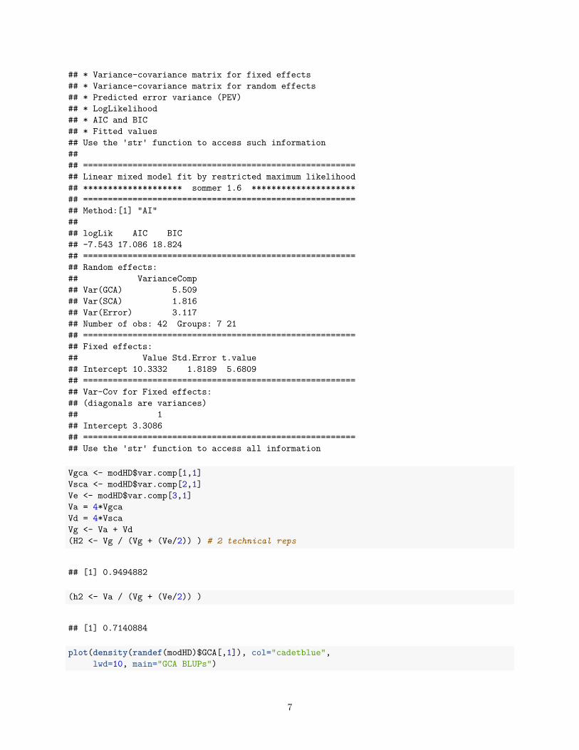
## * Variance-covariance matrix for fixed effects## * Variance-covariance matrix for random effects## * Predicted error variance (PEV)## * LogLikelihood## * AIC and BIC## * Fitted values## Use the 'str' function to access such information#### =======================================================## Linear mixed model fit by restricted maximum likelihood## ******************** sommer 1.6 *********************## =======================================================## Method:[1] "AI"#### logLik AIC BIC## -7.543 17.086 18.824## =======================================================## Random effects:## VarianceComp## Var(GCA) 5.509## Var(SCA) 1.816## Var(Error) 3.117## Number of obs: 42 Groups: 7 21## =======================================================## Fixed effects:## Value Std.Error t.value## Intercept 10.3332 1.8189 5.6809## =======================================================## Var-Cov for Fixed effects:## (diagonals are variances)## 1## Intercept 3.3086## =======================================================## Use the 'str' function to access all information

Vgca <- modHD$var.comp[1,1]Vsca <- modHD$var.comp[2,1]Ve <- modHD$var.comp[3,1]Va = 4*VgcaVd = 4*VscaVg <- Va + Vd(H2 <- Vg / (Vg + (Ve/2)) ) # 2 technical reps

## [1] 0.9494882

(h2 <- Va / (Vg + (Ve/2)) )

## [1] 0.7140884

plot(density(randef(modHD)$GCA[,1]), col="cadetblue",lwd=10, main="GCA BLUPs")

7

−6 −4 −2 0 2 4 6

0.00

0.05

0.10

0.15

GCA BLUPs

N = 7 Bandwidth = 1.076

Den

sity

3) Genome wide association analysis (GWAS) in diploids and tetraploids

With the development of modern statistical machinery the detection of markers associated to phenotypictraits have become quite straight forward. The days of QTL mapping using biparental populations exclusivelyare in the past. In this section we will show how to perform QTL mapping for diploid and polyploid organismswith complex genetic relationships. In addition we will show QTL mapping in biparental populations toclarify that the fact that is not required anymore doesn’t limit the capabilities of modern mixed modelmachinery.

First we will start doing the GWAS in a biparental population with 363 individuals genotyped with 2889SNP markers. This is easily done by creating the variance covariance among individuals and using it in therandom effect for genotypes. The markers are added in the W argument to fit the model of the form:

y = Xβ + Zu+Wg + ε

In this case Xβ is the fixed part only for the intercept, Zu is the random effect for genotypes with theadditive relationship matrix (A) as the variance-covariance of the random effect, Wg is the marker matrixand the effects of each marker. This is done in this way:

data(CPdata)CPpheno <- CPdata$phenoCPgeno <- CPdata$geno### look at the datahead(CPpheno); CPgeno[1:5,1:4]

## color Yield FruitAver Firmness

8

## 3 0.10075269 154.67 41.93 588.917## 4 0.13891940 186.77 58.79 640.031## 5 0.08681502 80.21 48.16 671.523## 6 0.13408561 202.96 48.24 687.172## 7 0.13519278 174.74 45.83 601.322## 8 0.17406685 194.16 44.63 656.379

## scaffold_50439_2381 scaffold_39344_153 uneak_3436043 uneak_2632033## P003 0 0 0 1## P004 0 0 0 1## P005 0 -1 0 1## P006 -1 -1 -1 0## P007 0 0 0 1

y <- CPpheno$color # responseZa <- diag(length(y)) # inidence matrix for random effectA <- A.mat(CPgeno) # additive relationship matrixETA.A <- list(add=list(Z=Za,K=A)) # create random componentans.A <- mmer(y=y, Z=ETA.A, W=CPgeno, silent=TRUE) # fit the model

## Estimating variance components#### Performing GWAS## Running additive model

0 500 1000 1500 2000 2500 3000

02

46

810

additive model

Marker index

−lo

g10(

p)

9

Now we will show how to do GWAS in a tetraploid using potato data. Is not very different from diploids. Weonly need to pay attention to the ploidy argument in the atcg1234 and A.mat functions. In addition, whenrunning the mmer model there is more models that can be implemented according to Rosyara et al. (2016).

data(PolyData)genotypes <- PolyData$PGenophenotypes <- PolyData$PPheno## convert markers to numeric formatnumo <- atcg1234(data=genotypes, ploidy=4, silent = TRUE); numo[1:5,1:5]; dim(numo)

## Obtaining reference alleles## Checking for markers with more than 2 alleles. If found will be removed.## Converting to numeric format## Calculating minor allele frequency (MAF)## Imputing missing data with mode

## c2_41437 c2_24258 c2_21332 c2_21320 c2_21318## A96104-2 1 2 2 4 0## A97066-42 2 3 2 4 1## ACBrador 2 4 2 4 0## ACLPI175395 0 4 0 4 0## ADGPI195204 0 4 0 4 0

## [1] 221 3521

# get only plants with both genotypes and phenotypescommon <- intersect(phenotypes$Name,rownames(numo))marks <- numo[common,]; marks[1:5,1:5]

## c2_41437 c2_24258 c2_21332 c2_21320 c2_21318## A97066-42 2 3 2 4 1## ACBrador 2 4 2 4 0## AdirondackBlue 2 2 2 4 1## AF2291-10 0 4 2 4 0## AF2376-5 1 3 2 4 0

phenotypes2 <- phenotypes[match(common,phenotypes$Name),];phenotypes2[1:5,1:5]

## Name total_yield chip_color tuber_eye_depth tuber_shape## 1 A97066-42 13.10 2.35 3.03 4.71## 2 ACBrador 15.56 2.63 4.37 3.59## 3 AdirondackBlue 11.77 2.82 3.76 4.07## 4 AF2291-10 13.43 1.50 4.50 2.81## 5 AF2376-5 12.58 1.83 4.50 2.81

# Additive relationship matrix, specify ploidyyy <- phenotypes2$tuber_shapeK1 <- A.mat(marks, ploidy=4)Z1 <- diag(length(yy))ETA <- list( list(Z=Z1, K=K1)) # random effects for genotypes

10

# run the modelmodels <- c("additive","1-dom-alt","1-dom-ref","2-dom-alt","2-dom-ref")ans2 <- mmer(y=yy, Z=ETA, W=marks, method="EMMA",

ploidy=4, models=models[1], silent = TRUE)

## Estimating variance components#### Performing GWAS## Running additive model

0 500 1000 1500 2000 2500 3000 3500

02

46

8

additive model

Marker index

−lo

g10(

p)

summary(ans2)

#### Information contained in this fitted model:## * Variance components## * Residuals and conditional residuals## * BLUEs and BLUPs## * Inverse phenotypic variance(V)## * Variance-covariance matrix for fixed effects## * Variance-covariance matrix for random effects## * Predicted error variance (PEV)## * LogLikelihood## * AIC and BIC## * Fitted values

11

## Use the 'str' function to access such information#### =======================================================## Linear mixed model fit by restricted maximum likelihood## ******************** sommer 1.6 *********************## =======================================================## Method:[1] "EMMA"#### logLik AIC BIC## -192.5 387.0 390.3## =======================================================## Random effects:## VarianceComp## V(u) 0.60778## V(e) 0.03807## Number of obs: 187 Groups: 187## =======================================================## Fixed effects:## Value Std.Error t.value## Intercept 3.307861 0.014268 231.83## =======================================================## Var-Cov for Fixed effects:## (diagonals are variances)## 1## Intercept 2e-04## =======================================================## Use the 'str' function to access all information

4) Genomic selection

In this section we will use wheat data from CIMMYT to show how is genomic selection performed. This isthe case of prediction of specific individuals within a population. It basically uses a similar model of the form:

y = Xβ + Zu+ ε

and takes advantage of the variance covariance matrix for the genotype effect known as the additive relationshipmatrix (A) and calculated using the A.mat function to establish connections among all individuals and predictthe BLUPs for individuals that were not measured. The prediction accuracy depends on several factors suchas the heritability (h2), training population used (TP), size of TP, etc.

data(wheatLines)X <- wheatLines$wheatGeno; X[1:5,1:5]; dim(X)

## wPt.0538 wPt.8463 wPt.6348 wPt.9992 wPt.2838## [1,] -1 1 1 1 1## [2,] 1 1 1 1 1## [3,] 1 1 1 1 1## [4,] -1 1 1 1 1## [5,] -1 1 1 1 1

## [1] 599 1279

12

Y <- wheatLines$wheatPhenorownames(X) <- rownames(Y)# select environment 1y <- Y[,1] # response grain yieldZ1 <- diag(length(y)) # incidence matrixK <- A.mat(X) # additive relationship matrix# GBLUP pedigree-based approachset.seed(12345)y.trn <- yvv <- sample(1:length(y),round(length(y)/5))y.trn[vv] <- NAETA <- list(g=list(Z=Z1, K=K))ans <- mmer(y=y.trn, Z=ETA, method="EMMA", silent = TRUE) # kinship based

## Estimating variance components

cor(ans$u.hat$g[vv],y[vv])

## [1] 0.4885687

## maximum prediction value that can be achievedsqrt(ans$var.comp[1,1]/sum(ans$var.comp[,1]))

## V(u)## 0.5771923

5) Single cross prediction

When doing prediction of single cross performance the phenotype can be dissected in three main components,the general combining abilities (GCA) and specific combining abilities (SCA). This can be expressed with thesame model analyzed in the diallel experiment mentioned before:

y = Xβ + Zu1 + Zu2 + ZuS + ε

with:

u1 ~ N(0, K1σ2u1)

u2 ~ N(0, K2σ2u2)

us ~ N(0, K3σ2us)

And we can specify the K matrices. The main difference between this model and the full and half dialleldesigns is the fact that this model will include variance covariance structures in each of the three randomeffects (GCA1, GCA2 and GCA3) to be able to predict the crosses that have not ocurred yet. We will usethe data published by Technow et al. (2015) to show how to do prediction of single crosses.

data(Technow_data)

A.flint <- Technow_data$AF # Additive relationship matrix FlintA.dent <- Technow_data$AD # Additive relationship matrix DentM.flint <- Technow_data$MF # Marker matrix FlintM.dent <- Technow_data$MD # Marker matrix Dent

13

pheno <- Technow_data$pheno # phenotypes for 1254 single cross hybridspheno$hy <- paste(pheno$dent, pheno$flint, sep=":");head(pheno);dim(pheno)

## hybrid dent flint GY GM hy## 1 518.298 518 298 -8.04 -0.85 518:298## 2 518.305 518 305 -11.10 1.70 518:305## 3 518.306 518 306 -16.85 2.24 518:306## 4 518.316 518 316 2.08 -1.33 518:316## 5 518.323 518 323 5.65 -2.71 518:323## 6 518.327 518 327 -16.95 -0.52 518:327

## [1] 1254 6

# CREATE A DATA FRAME WITH ALL POSSIBLE HYBRIDSDD <- kronecker(A.dent,A.flint,make.dimnames=TRUE)

hybs <- data.frame(sca=rownames(DD),yield=NA,matter=NA,gcad=NA, gcaf=NA)hybs$yield[match(pheno$hy, hybs$sca)] <- pheno$GYhybs$matter[match(pheno$hy, hybs$sca)] <- pheno$GMhybs$gcad <- as.factor(gsub(":.*","",hybs$sca))hybs$gcaf <- as.factor(gsub(".*:","",hybs$sca))head(hybs)

## sca yield matter gcad gcaf## 1 513:316 10.02 -2.05 513 316## 2 513:323 6.97 -3.78 513 323## 3 513:330 NA NA 513 330## 4 513:336 NA NA 513 336## 5 513:340 NA NA 513 340## 6 513:341 NA NA 513 341

# CREATE INCIDENCE MATRICESZ1 <- model.matrix(~gcad-1, data=hybs)Z2 <- model.matrix(~gcaf-1, data=hybs)# SORT INCIDENCE MATRICES ACCORDING TO RELATIONSHIP MATRICES, REAL ORDERSreal1 <- match( colnames(A.dent), gsub("gcad","",colnames(Z1)))real2 <- match( colnames(A.flint), gsub("gcaf","",colnames(Z2)))Z1 <- Z1[,real1]Z2 <- Z2[,real2]# RUN THE PREDICTION MODELy.trn <- hybs$yieldvv1 <- which(!is.na(hybs$yield))vv2 <- sample(vv1, 100)y.trn[vv2] <- NAETA2 <- list(GCA1=list(Z=Z1, K=A.dent), GCA2=list(Z=Z2, K=A.flint))anss2 <- mmer(y=y.trn, Z=ETA2, method="EM", silent=TRUE)

## Estimating variance components

14

summary(anss2)

#### Information contained in this fitted model:## * Variance components## * Residuals and conditional residuals## * BLUEs and BLUPs## * Inverse phenotypic variance(V)## * Variance-covariance matrix for fixed effects## * Variance-covariance matrix for random effects## * Predicted error variance (PEV)## * LogLikelihood## * AIC and BIC## * Fitted values## Use the 'str' function to access such information#### =======================================================## Linear mixed model fit by restricted maximum likelihood## ******************** sommer 1.6 *********************## =======================================================## Method:[1] "EM"#### logLik AIC BIC## -4998 9999 10004## =======================================================## Random effects:## VarianceComp## Var(GCA1) 16.01## Var(GCA2) 11.16## Var(Error) 17.71## Number of obs: 1154 Groups: 123 86## =======================================================## Fixed effects:## Value Std.Error t.value## Intercept 0.24778 0.20360 1.2169## =======================================================## Var-Cov for Fixed effects:## (diagonals are variances)## 1## Intercept 0.0415## =======================================================## Use the 'str' function to access all information

cor(anss2$fitted.y[vv2], hybs$yield[vv2])

## [1] 0.8778897

In the previous model we only used the GCA effects (GCA1 and GCA2) for practicity, altough it’s beenshown that the SCA effect doesn’t actually help that much in increasing prediction accuracy and increase alot the computation intensity required since the variance covariance matrix for SCA is the kronecker productof the variance covariance matrices for the GCA effects, resulting in a 10578x10578 matrix that increases in avery intensive manner the computation required.

15

A model without covariance structures would show that the SCA variance component is insignificant comparedto the GCA effects. This is why including the third random effect doesn’t increase the prediction accuracy.

Literature

Covarrubias-Pazaran G (2016) Genome assisted prediction of quantitative traits using the R package sommer.https://cran.rstudio.com/web/packages/sommer/

Bernardo Rex. 2010. Breeding for quantitative traits in plants. Second edition. Stemma Press. 390 pp.

Gilmour et al. 1995. Average Information REML: An efficient algorithm for variance parameter estimation inlinear mixed models. Biometrics 51(4):1440-1450.

Henderson C.R. 1975. Best Linear Unbiased Estimation and Prediction under a Selection Model. Biometricsvol. 31(2):423-447.

Kang et al. 2008. Efficient control of population structure in model organism association mapping. Genetics178:1709-1723.

Lee et al. 2015. MTG2: An efficient algorithm for multivariate linear mixed model analysis based on genomicinformation. Cold Spring Harbor. doi: http://dx.doi.org/10.1101/027201.

Searle. 1993. Applying the EM algorithm to calculating ML and REML estimates of variance components.Paper invited for the 1993 American Statistical Association Meeting, San Francisco.

Yu et al. 2006. A unified mixed-model method for association mapping that accounts for multiple levels ofrelatedness. Genetics 38:203-208.

Abdollahi Arpanahi R, Morota G, Valente BD, Kranis A, Rosa GJM, Gianola D. 2015. Assessment of baggingGBLUP for whole genome prediction of broiler chicken traits. Journal of Animal Breeding and Genetics132:218-228.

Tunnicliffe W. 1989. On the use of marginal likelihood in time series model estimation. JRSS 51(1):15-27.

16