genetics of small populations: the case of the laysan finch

Case Studies in Ecology and Evolution DRAFT

D. Stratton 2008 1

2 Genetics of Small Populations: the case of the Laysan Finch

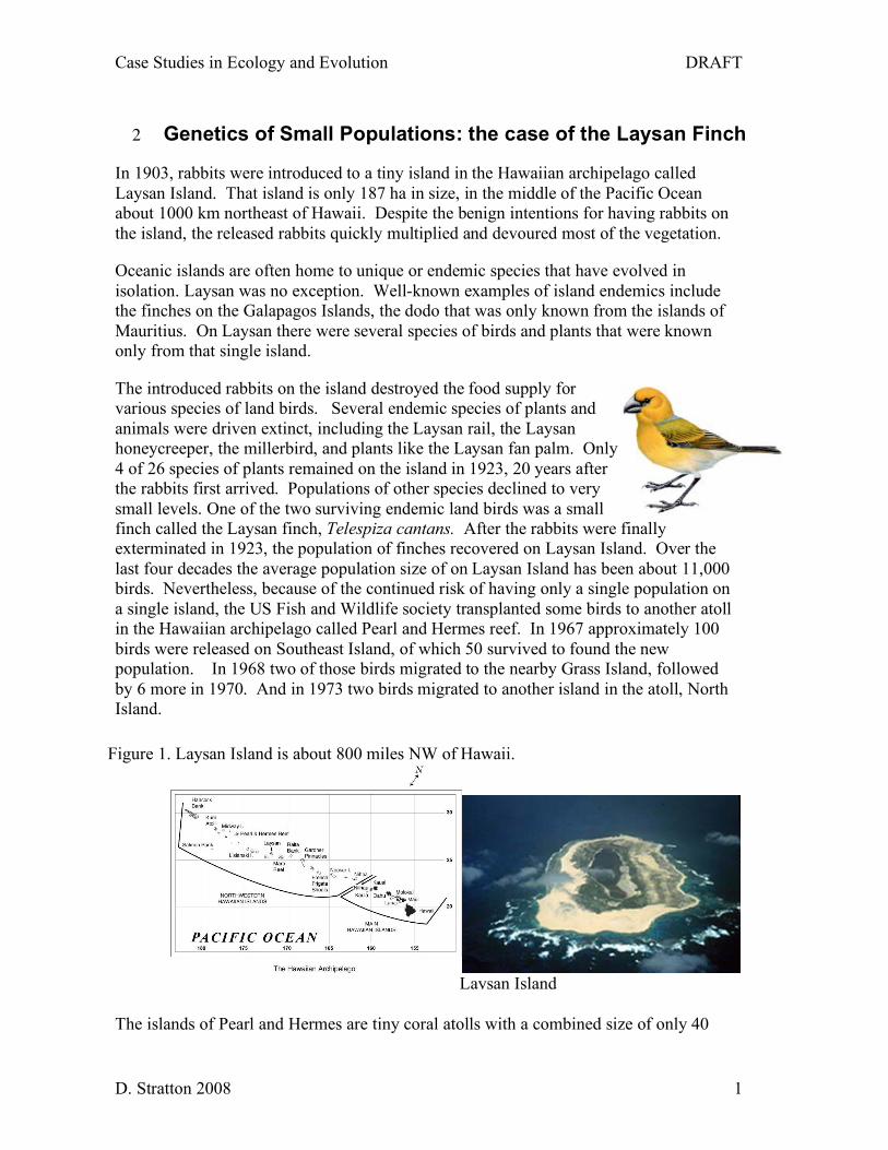
In 1903, rabbits were introduced to a tiny island in the Hawaiian archipelago called

Laysan Island. That island is only 187 ha in size, in the middle of the Pacific Ocean

about 1000 km northeast of Hawaii. Despite the benign intentions for having rabbits on

the island, the released rabbits quickly multiplied and devoured most of the vegetation.

Oceanic islands are often home to unique or endemic species that have evolved in

isolation. Laysan was no exception. Well-known examples of island endemics include

the finches on the Galapagos Islands, the dodo that was only known from the islands of

Mauritius. On Laysan there were several species of birds and plants that were known

only from that single island.

The introduced rabbits on the island destroyed the food supply for

various species of land birds. Several endemic species of plants and

animals were driven extinct, including the Laysan rail, the Laysan

honeycreeper, the millerbird, and plants like the Laysan fan palm. Only

4 of 26 species of plants remained on the island in 1923, 20 years after

the rabbits first arrived. Populations of other species declined to very

small levels. One of the two surviving endemic land birds was a small

finch called the Laysan finch, Telespiza cantans. After the rabbits were finally

exterminated in 1923, the population of finches recovered on Laysan Island. Over the

last four decades the average population size of on Laysan Island has been about 11,000

birds. Nevertheless, because of the continued risk of having only a single population on

a single island, the US Fish and Wildlife society transplanted some birds to another atoll

in the Hawaiian archipelago called Pearl and Hermes reef. In 1967 approximately 100

birds were released on Southeast Island, of which 50 survived to found the new

population. In 1968 two of those birds migrated to the nearby Grass Island, followed

by 6 more in 1970. And in 1973 two birds migrated to another island in the atoll, North

Island.

The islands of Pearl and Hermes are tiny coral atolls with a combined size of only 40

Figure 1. Laysan Island is about 800 miles NW of Hawaii.

Laysan Island


D. Stratton 2008 2

ha. The highest point of land is only 3 m above sea level and some parts are

occasionally submerged. So the population sizes on those tiny islands have never gotten

large in the 4 decades since they were founded. On Southeast Island the population

grew rapidly and has since fluctuated around an average of about 350 birds, whereas the

populations on North Island and Grass Island have hovered around 30-50. In contrast,

the original population on Laysan averages about 11,000 birds.

Figure 2. Population size fluctuations on the smaller islands of Pearl and Hermes Reef.

Just as small populations of birds have a risk of extinction, there is always a chance of

some alleles going extinct in any small population. Because the allelic diversity of a

population is one important measure of the evolutionary potential of that population,

conservation biologists have been very concerned about the rate of loss of genetic

diversity in small populations. The population of Laysan Finches on Pearl and Hermes

were all founded by small numbers of birds, and those populations have only increased

to moderate size. What impact will small population size have on the genetic variation

of those populations?

To answer that question we will first look at the sampling theory for alleles in finite

populations and examine a classic laboratory experiment in some detail. After that,

we’ll return to the Laysan Finch and answer our question about the genetic

consequences of small population size.

2.1 Genetic Drift

In deriving the Hardy Weinberg Equilibrium we assumed that the population size was

large enough that we could ignore random sampling and look only at the expected

frequency of alleles and genotypes. Under HWE we expect the allele frequency to

remain constant. However, small samples of gametes from the gamete pool may

deviate by chance from the sample as a whole. In finite populations there may be

slight deviations in the number of A or a alleles that are actually passed on to the next

generation, so allele frequencies may deviate slightly from the expected frequency, just

by chance. We call that process of random changes in allele frequency due to

sampling in small populations genetic drift.


D. Stratton 2008 3

Genetic drift occurs whenever the population has finite size—in other words in all

populations, all of the time. But drift most important when population sizes are very

small.

There are several ways that the sampling effects manifest themselves in small

populations. The most important is that in any small number of trials the results may not

exactly match the expectations. For example, imagine flipping a coin. Even though we

expect to get "heads" half of the time, if we flip two coins there is a moderately high

probability of getting either two heads or two tails. On the other hand if we flip 100

coins, the observed frequency of "heads" will be much closer to 0.5. In terms of

population genetics, even though we expect allele frequency to stay constant, in small

populations it is not unusual to find small deviations in allele frequency from one

generation to the next. That sampling effect is genetic drift.

2.2 Assumptions:

We will keep all of the assumptions that were used in deriving the Hardy Weinberg

equilibrium, EXCEPT now have finite population size. In particular, we will still

assume that there are no fitness differences among alleles, that the population is closed,

so there is no migration into or out of the population, and that there is no addition of

genetic variation by mutation. And there is still random mating, so genotypes will be

approximately in HW proportions at any given time. But in a finite population, the

actual frequencies of genotypes and alleles will not always exactly match the HW

expectations. The result is that, from the finite sampling process alone, allele

frequencies will by pure chance deviate slightly from their expectations, which leads to

a slow change in the allele frequencies over time.

Basic assumptions, modified for finite populations:

! Random mating. Individuals mate at random with respect to the locus in

question.

! Closed population. There is no migration into or out of the population.

! No mutation.

! No selection. All individuals have the same expected survival and fecundity.

! Finite population size. This is the only assumption that has been modified.

2.3 The sampling process

To keep things simple, we will start by keeping track of gametes only (remember our

conceptual model of a gamete pool?). We can do that because we assume there is

random mating, which just means that gametes are chosen at random from the pool of

possible gametes. If the population size stays constant, then

each gamete will (on average) leave exactly 1 descendant.

However, by chance some will be copied more than once and

some will not leave any descendants at all.

Each time an allele fails to be copied, just by chance, that

copy is lost from the population and leaves no further

Time


D. Stratton 2008 4

descendants. Eventually, if this process continues long enough, all alleles in a population

can trace their ancestry to a single allele.

Example: three simulations of drift in a tiny population with 2N=8 alleles. Assume that

the population starts with two types of alleles (red and blue) and the initial frequency of the

red allele is 3/8. To be explicit we’ll give each founder allele a unique number. In the first

generation all 8 of those alleles are present. We assume that these alleles are all selectively

neutral, meaning that each allele has an equal probability of being copied each generation.

In each of those three replicates, all but one allele are eventually lost from the population.

When only a single allele remains in the population we say that it has become “fixed” for

that allele. Although the general pattern and time to fixation is similar in the three replicates,

a different one of the eight original alleles was fixed in each simulation.

Each of the 8 initial alleles has an equal chance of being fixed in the population. Because the

population starts with more blue alleles than red alleles, a blue allele is more likely to be the

one that eventually goes to fixation.

Repicate 1 Replicate 2 Replicate 3

11222222555555555555 22222255555555555555 32222255555555555555 44445255555555555555 55555555555555555555 66555555555555555555 76555555555555555555 87655555555555555555

time ---->

12222222244444444444 24244444444444444444 34444444444444444444 45554444444444444444 55554444444444444444 66555444444444444444 77665444444444444444 88666554444444444444

time ---->

11111111111111111111 22311111111111111111 33331111111111111111 43333111111111111111 56333111111111111111 67363311111111111111 77663313111111111111 88776333333333111111

time ---->

If all of the initial alleles have an equal chance of being fixed and if we start with 3 red

and 5 blue alleles, what is the probability that the population is eventually fixed for a

blue allele?

________________

General result: The probability of fixation of an allele is equal to its frequency in the

population.

Prob(fixation) = p (eq 2.1)

Alleles that start at high frequency have a higher probability of eventually going to fixation

than alleles that start at low frequency.


D. Stratton 2008 5

For every new mutation the initial frequency of the new mutant is

!

p =1

2N. In a population

with 2N=100 alleles, what is the probability that the new mutation will eventually become

fixed in the population? _________________

What is the probability that the new mutation will not become fixed (i.e. that it will go

extinct)? _________________

slightly harder: what is the probability that the new mutation immediately goes extinct in the first generation?

2.4 Rate of decrease in heterozygosity

Diversity is lost in all finite populations as one allele eventually goes to fixation. How fast is

it lost?

One measure of variation is the heterozygosity (the proportion of heterozygotes in the

population).

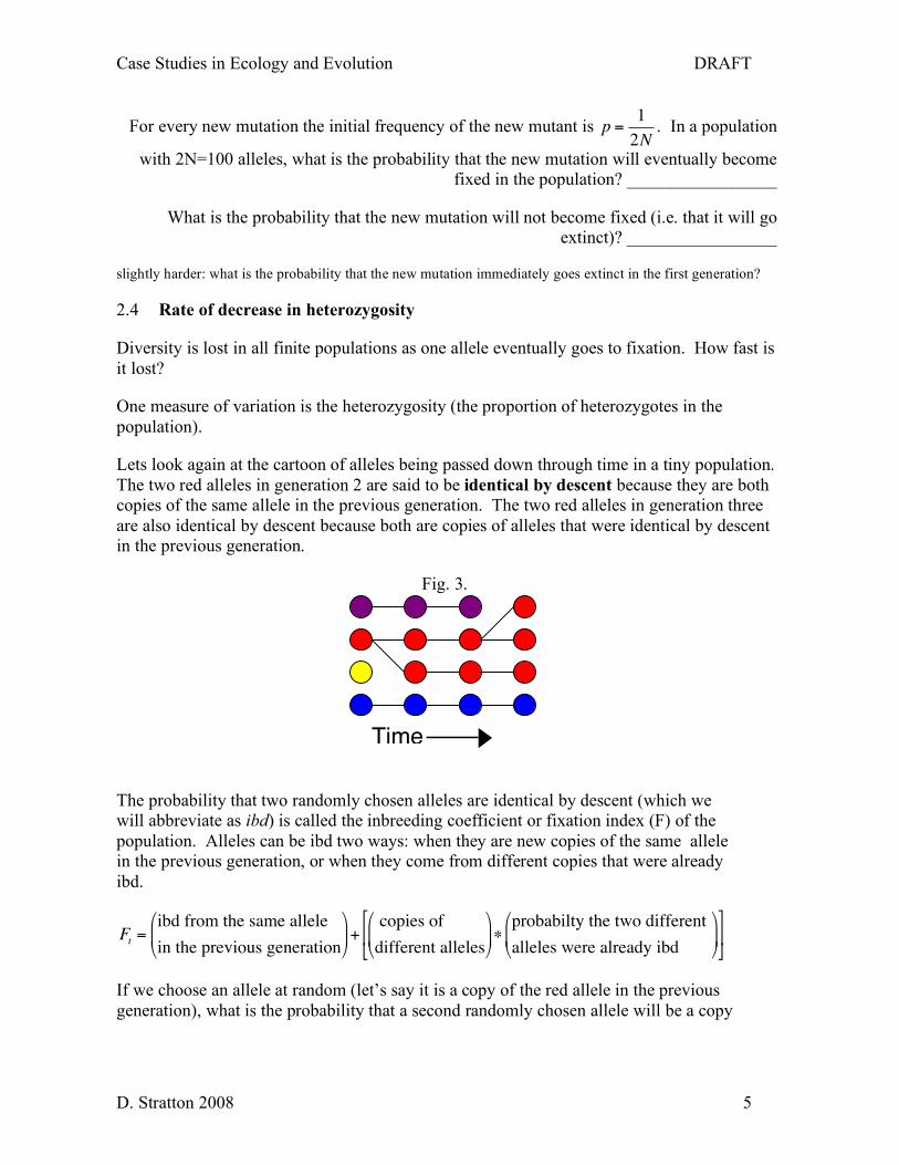
Lets look again at the cartoon of alleles being passed down through time in a tiny population.

The two red alleles in generation 2 are said to be identical by descent because they are both

copies of the same allele in the previous generation. The two red alleles in generation three

are also identical by descent because both are copies of alleles that were identical by descent

in the previous generation.

Fig. 3.

The probability that two randomly chosen alleles are identical by descent (which we

will abbreviate as ibd) is called the inbreeding coefficient or fixation index (F) of the

population. Alleles can be ibd two ways: when they are new copies of the same allele

in the previous generation, or when they come from different copies that were already

ibd.

!

Ft=

ibd from the same allele

in the previous generation

"

# $

%

& ' +

copies of

different alleles

"

# $

%

& ' (

probabilty the two different

alleles were already ibd

"

# $

%

& '

)

* +

,

- .

If we choose an allele at random (let’s say it is a copy of the red allele in the previous

generation), what is the probability that a second randomly chosen allele will be a copy

Time


D. Stratton 2008 6

of that same red allele? If there are N individuals there are 2N total alleles, so the

probability that it comes from the same particular allele is 1 / 2N

What if instead they are ibd from some previous event? The probability that two

randomly chosen alleles come from different parent alleles is (1-1/2N) and the

probability that those parents were already ibd is simply the inbreeding coefficient in

the previous generation, Ft-1.

So our overall expression for the inbreeding coefficient is:

!

Ft=1

2N+ 1"

1

2N

#

$ %

&

' ( Ft"1 (eq 2.2)

That is the probability that the two gametes are copies of the same allele in the previous

generation (1/2N) or (+) they came from two different alleles (1-1/2N) and (*) those alleles

were already ibd (Ft-1).

2.4.1 Heterozygosity

We started by looking at the increase in the fixation index because that is easy to visualize.

But the math is actually a bit easier if we keep track of the heterozygosity instead. Since the

expected heterozygosity (H) is the probability that two random alleles are not ibd,

H= 1-F (eq 2.3)

Recasting equation ?? in terms of H, you can show that

!

Ht+1 = 1"

1

2N

#

$ %

&

' ( Ht

(eq. 2.4)

and the change in heterozygosity is

!

"H = #1

2NH

t (eq. 2.5)

Each generation the average heterozygosity should decrease by a constant percentage,

!

1

2N.

That means that after t generations of genetic drift, the heterozygosity will be:

!

Ht= 1"

1

2N

#

$ %

&

' (

t

H0 (eq. 2.6)

2.5 Divergence among populations

The replicate populations in the simulations in figure ?? show another general feature of

genetic drift. Even though all of the populations start with identical allele frequencies, they

gradually diverge over time. If you start many replicate populations with two alleles A and

a, and p is the frequency of allele A, then p of them will eventually become fixed for A and

(1-p) will become fixed for allele a.


D. Stratton 2008 7

Replicate populations will tend to diverge in allele frequency as a particular allele gets fixed

in some populations and goes extinct in others. The rate of divergence is much faster in

small populations than large populations.

Figure __. Drift in allele frequency, p=0.5; In each case there are 10 replicate populations

of a given population size, all starting with p=0.5. Even with a population size of 1000 the

allele frequencies in the replicate populations do not remain exactly at p=0.5; however the

changes in allele frequency are negligible compared to the changes in small populations.

Fig 2.4. Change in allele frequency by drift among replicate populations of different sizes.

Once an allele goes extinct, that allele is lost forever. So, if this process is allowed to

continue long enough the allele frequency will eventually be either 0 or 1 in all

populations.

Large pops show 1) less variation in allele frequency over time 2) longer time to

fixation.

2.6 A laboratory study of genetic drift.

One of the best tests of genetic drift comes from a laboratory experiment done by Peter Buri

in the 1950s. He was a student of Sewall Wright’s at the University of Chicago. The design

of the experiment was elegantly simple: he set up over 100 replicate populations of 16 fruit

flies and followed each population for many generations to examine the changes in allele

frequency.

All of the populations started out with 8 males and 8 females that were all heterozygous for

an eye color mutation. He could easily keep track of the different genotypes by their eye

color. Homozygotes for the mutant bw allele had white eyes, homozygotes for the bw75

allele had bright red eyes and the heterozygotes had light orange eyes. Each generation he

collected the first 8 males and the first 8 females in his sample, counted the numbers of each

eye-color genotype, and used them as parents to start the next generation. In that way the

population size was precisely maintained at 16 flies for the entire experiment.

Because he wanted to look at the neutral changes in allele frequency as a result of genetic

drift, he was careful to show that the eye color locus had no measurable effect on the fitness


D. Stratton 2008 8

of the flies. He did that by starting some large populations about 1000-2000 flies that had an

equal frequency of bw and bw75 alleles and followed those populations for several weeks.

There was no systematic change in allele frequency over that time period.

Figure 2.5 shows the results for one of his experiments. There were a total of 107 replicate

populations. In each

population of 16 flies

there were a total of 32

alleles, so there could be

anywhere between 0 to

32 copies of the bw75

allele in each population.

At generation 0, all of

the flies were

heterozygous bw/bw75

so 107/107 populations

had exactly 16 copies of

the bw75 allele. In

generation 1, most

populations had

intermediate numbers of the bw75 allele, but one population had only 7 copies and one

population had as many as 22. By generation 10, some of the populations had lost the bw75

allele completely and others had lost the bw allele. By generation 19, many more of the

populations had become fixed for one allele or the other.

! What do you predict the distribution to be if this experiment continued for many

more generations?

! What is the allele freq at the beginning of the experiment? ______________

! Approximately what is the average allele frequency (among all populations) at

the end of the experiment? ________________

Table 2.1. Changes in Heterozygosity over time during Buri’s experiment.

Average frequency of

heterozygotes over all

replicate lines

Expected Heterozygosity

Generation H He

1 0.514 0.500

2 0.464

3 0.504

4 0.456


D. Stratton 2008 9

The expected heterozygosity is 0.5 in generation 1 and there was a constant population of

size N=16 flies. Using equation 2.6, what is the expected heterozygosity in generation 11,

after 10 generations of drift?

He=_____________________

What is the expected heterozygosity in generation 19, after 18 generations of drift?

He=_____________________

How does that compare to the observed heterozygosity?

Buri’s populations lost genetic variation much faster than would be predicted for a

population of 16 flies. He repeated the whole experiment with a second series of

populations and found essentially the same results.

5 0.448

6 0.428

7 0.403

8 0.402

9 0.358

10 0.348

11 0.325 He, 11 =

12 0.305

13 0.263

14 0.255

15 0.216

16 0.202

17 0.210

18 0.197

19 0.183 He, 19 =


D. Stratton 2008 10

2.7 Effective population size

Why don’t the results of Buri’s experiment match our expectations? When the results of an

experiment don’t match the expectations of the model, we need to go back and examine the

model assumptions. In our idealized population, we modeled drift by assuming individuals

were identical and mate completely at random (by that we meant that they produce an

infinite number of gametes, from which we draw pairs of alleles at random). An implicit

assumption of that model was that there were no sexes: we did not keep track of where the

two random gametes came from. They could even have come from the same individual. In

Buri’s experiment (and most real populations we would be interested in) each individual

must have one male and one female parent..

Another implicit assumption of that sampling process was that the number of offspring

produced by each individual would come from a binomial distribution with mean=1. In

many real populations, some individuals are more fecund than others. Large females may

lay more eggs than small females, or dominant males may sire more offspring than

subordinate males.

In either case, the effective population size (Ne) may be smaller than the actual number of

individuals.

How can we calculate Ne? We can use equation 2.6, substituting and initial heterozygosity

of 0.5 in generation 1 and the observed heterozygosity of 0.183 18 generations later and

then solve for Ne.

!

0.183= 1"1

2Ne

#

$ %

&

' (

18

0.5

Take logs of both sides to get rid of the exponent:

!

ln(0.183) =18 ln 1"1

2Ne

#

$ %

&

' ( + ln(0.5)

so Ne =9.2

In Buri’s experiment, even though the populations had 16 flies, they lost genetic variance as

if they had only 9.2 flies in each. Thus we can say that the effective population size in this

experiment was 9.2.

Figure 2.6 Observed and predicted decline in heterozygosity in Buri's experiment.


D. Stratton 2008 11

What are some of the biological reasons why Ne differs from N? We don’t know the precise

answer for Buri’s flies, but theory has shown that several factors can influence the effective

size of a population. Here are a few theoretical results:

2.7.1 Unequal sex ratio

When the number of males (Nm) and females (Nf) in a population are not equal, then the

effective population size can be shown to be approximately

!

Ne "4NmN f

Nm + N f

(eq. 2.7)

! Assume there 1000 females (Nf=1000) but only a single male is responsible for all of

the matings (Nm=1). What is Ne for that population?

! Ne=_________________

2.7.2 Variation in family size

In many populations, some individuals will be highly fecund and others may not reproduce

at all. That is especially true for animals with strong dominance hierarchies (such as

wolves) where some individuals sire most of the offspring, and species with indeterminate

growth (such as plants), where a few large individuals may be responsible for most of the

seed production in the population. In that case there will be a much larger variance in

family size that we assumed in our ideal population.


D. Stratton 2008 12

When there is variation in family size, Ne is approximately

!

Ne"4N # 2

v+ 2 (eq. 2.8)

where v is the variance in the number of offspring produced by different individuals.

! One estimate of variance in egg number for salmon was 69. In a population of 1000

spawners, how much smaller will the effective population size be than the apparent

number of spawners?

! Ne= _________________

! What if you could ensure that all individuals have exactly the same number of

offspring? (perhaps by managing a captive population in a zoo). In that case the

variance in family size will be zero. What will be the effective population size?

! Ne= _________________

2.7.3 Variation in population size over time

When population size varies over time, the average effective size of the population is

affected more by the periods when populations are small than when they are large. The

average effective size is approximately the harmonic mean of population size:

!

1

Ne

= Average 1N( )

or after t generations

!

Ne

=t

1

N1

+ 1

N2

+ ...+ 1

Nt

(eq. 2.9)

What if the population size is constant: i.e. if over 5 yrs N={100,100,100,100,100}?

Ne=__________________

What if the population starts with a single individual but then immediately stabilizes at a

larger size? i.e. over 5 yrs N={1,100,100,100,100}

Ne=__________________

2.8 Main feature of drift:

! Loss of variation within populations

o as all alleles except one eventually go extinct


D. Stratton 2008 13

! Increase in variation among populations

o as different alleles become common in different populations

! Evolution

o because allele frequencies change over time

o note that we are not implying adaptation . . . just evolution.

2.9 How does this relate to the Laysan Finch?

Biologists continued to study the Laysan Finches after they were introduced to Pearl and

Hermes reef. In addition to censusing the population size on those islands, they occasionally

collected blood samples from some of the birds to monitor any changes in genetic diversity

in those populations.

Again the heterozygosity of a population is a good measure of genetic diversity. The

observed heterozygosity is just the proportion of heterozygotes: the number of heterozygous

individuals divided by the total number of individuals. When there are two alleles at a locus

we have already seen that the expected proportion of heterozygotes under random mating is

simply 2pq. But how do you calculate the expected heterozygosity when there are more

than two alleles? With three alleles (p, q, r) there are three classes of heterozygotes, so you

could just sum the frequencies: H=2pq + 2pr + 2qr. But with more alleles the number of

different heterozygous combinations increases rapidly. For 5 alleles there are 10 possible

heterozygotes to consider. When there are many alleles it is easiest to calculate the

heterozygosity as the proportion of individuals that are not homozygous.

Each homozygous genotype has a frequency pi2, where pi is the frequency of the i

th allele.

All other genotypes are heterozygous. Therefore, the expected frequency of heterozygotes

(using the not rule to find the frequency of genotypes that are not homozygous) is:

!

Hexp =1" pi2# (eq. 2.10)

Here are some results for one microsatellite locus, for which 5 different alleles were

observed.

Table 2 Alleles

Locus

Tc12B5E N 125 127 135 137 139

Number of

heterozygotes Hobs Hexp

N alleles in

population

Laysan 44 0.295 0.034 0.545 0.114 0.011 25 0.568 0.602 5

Southeast 43 0.116 0.116 0.756 0.012 0 19 0.442 0.401 4

North 43 0.128 0 0.791 0.081 0 16

Grass 36 0 0 1.000 0 0 0


D. Stratton 2008 14

What are the observed and expected heterozygosities for North Island and Grass Island?

They looked at a total of 9 loci. Averaged across all of those loci, here is what they found.

Table 2.3

Island Average H Ne

Laysan 0.535

Southeast 0.491 58.5

North 0.341 11.3

Grass 0.401

Using the heterozygosity of the Laysan island population as the initial heterozygosity (H0),

and assuming that there have been approximately t=10 generations since the founding of the

other three populations, what is the effective population size of each of the small islands?

The arithmetic is a little tedious, but it is possible to calculate the effective population size

on each island from equation 2.6, as in section 2.7, above. For example, on Southeast Island,

!

Ht

= 1"1

2N

#

$ %

&

' (

t

H0

!

Ln(H

t

H0

) = t " Ln 1#1

2N

$

% &

'

( )

Ln(0.491

0.535) =10 " Ln 1#

1

2Ne

$

% &

'

( )

#0.0858

10= Ln 1#

1

2Ne

$

% &

'

( )

e

#0.0858

10 = 0.9829 =1#1

2Ne

0.9914 =1#1

2Ne

Ne

=1

2(1# 0.9914)= 58.5


D. Stratton 2008 15

Using similar logic, what is the effective population size on Grass Island?

Remember that fluctuating population size is one of the factors that may affect Ne.

Unfortunately we don’t have yearly censuses of the population size on those islands. Here

are the data that are available (from Fig 2.2).

Table 2.4 Population size (N)

Year

Southeast

Island

North

Island

Grass

Island

1967 50

1968 223 2

1969 166

1970 183 8

1971 480

1972 375 8

1973 730 2 8

1974 436

1975

1976

1977

1978 202 92 16

1979

1980

1981

1982

1983 524 354

1984 515 153 30

1985 591 194 46

1986 434 272 52

1987 181 56 26

1988 156 36 17

1989

1990 67

1991

1992

1993

1994

1995

1996

1997

1998 350 30

Average of

(1/N) 0.0045 0.065

Ne 222 15.4


D. Stratton 2008 16

Those data are pretty sparse. Still, we can calculate the harmonic mean of the counts that we

do have and use that for another (rough) estimate of Ne.

What is the effective population size on Grass Island by this method?

_____________________

How do those estimates compare to the estimates of effective size based on changes in

heterozygosity?

Finally, compare those estimates of Ne with the simulations of drift in Figure 2.4 to get a

rough idea of how long those small populations are likely to maintain their genetic diversity

if the populations continue as they are now.

Answers: p 4. Prob(blue)=5/8

p 5. Prob(fixed)=1/2N; Prob(extinct)=1-1/2N

p 8. Eventually all lines will become fixed for one allele or the other. Starting allele frequency is 0.5; The Average allele

frequency at the end of the experiment is still about 0.5

p 9. H(11) = 0.36 H(19) =0.28, both higher than the observed H.

p 11 Ne = 3.99

p 12 Ne (salmon) = 56.3; Ne (equal) = 2N-1; Ne (constant size) =100; Ne(bottleneck) =4.8

p 13 North Island: Ho=0.372 He =0.351; Grass Island: Ho=0 He=0

p 14 Grass Island Ne=17.6

p 16 Ne=9.6 -- not really close to the other estimate, but a similar order of magnitude.

For Ne of 10 they will lose most of their genetic variation in around 20 generations or so.

genetics of small populations: the case of the laysan finch

Documents