1

Genomic 3D-compartments emerge from unfolding

mitotic chromosomes

Rajendra Kumar1,2, Ludvig Lizana1,2*, Per Stenberg3,4*

1 Integrated Science Lab, Umeå University, Sweden. 2 Department of Physics, Umeå University, Sweden. 3 Department of Ecology and Environmental Science (EMG), Umeå University, Sweden. 4 Division of CBRN Security and Defence, FOI-Swedish Defence Research Agency, Umeå, Sweden * To whom correspondence should be addressed. Email: ludvig.lizana@umu.se,

per.stenberg@umu.se (+46 90 7856777)

Keywords: nuclear structure, polymer simulation, chromosome decondensation, Hi-C

Acknowledgements This project was funded by the Kempe Foundation (grant number JCK-1347 to LL and PS) and the Knut

and Alice Wallenberg foundation (grant number 2014-0018, to EpiCoN, co-PI: PS). The simulations

were performed on resources provided by the Swedish National Infrastructure for Computing (SNIC) at

HPC2N Umeå, Sweden.

2

Abstract The 3D organisation of the genome in interphase cells is not a randomly folded polymer. Rather,

experiments show that chromosomes arrange into a network of 3D compartments that correlate with

biological processes, such as transcription, chromatin modifications, and protein binding. However,

these compartments do not exist during cell division when the DNA is condensed, and it is unclear how

and when they emerge. In this paper, we focus on the early stages after cell-division as the

chromosomes start to decondense. We use a simple polymer model to understand the types of 3D

structures that emerge from local unfolding of a compact initial state. From simulations, we recover 3D

compartments, such as TADs and A/B compartments, that are consistently detected in Chromosome

Capture Experiments across cell types and organisms. This suggests that the large-scale 3D

organisation is a result of an inflation process.

3

Introduction Apart from the bare challenge of packing a long DNA polymer into a small cell nucleus without heavy

knotting, the DNA must fold in 3D to allow nuclear processes, such as gene activation, repression and

transcription, to run smoothly. By how much the DNA folding patterns influences these processes, and

by how much they influence human health, is currently attracting a lot of attention in the scientific

community (Cremer and Cremer 2001; Fullwood et al. 2009; Gondor 2013; Krijger and de Laat 2016;

Schneider and Grosschedl 2007; Sexton et al. 2007).

To better understand DNA’s 3D organization, researchers developed various Chromosome

Conformation Capture Methods. The most recent incarnation, the Hi-C method (Lieberman-Aiden et al.

2009), measures contact probabilities between all pairs of loci in the genome. Across cell types and

organisms, Hi-C repeatedly detects two types of co-existing megabase scale structures. First, all

chromosome loci seem to belong to one of two so-called A/B compartments (Lieberman-Aiden et al.

2009), where the chromatin in one compartment is generally more open, accessible, and actively

transcribed than the other. Second, linear subsections of the genome assemble into topological

domains (Dixon et al. 2012; Nora et al. 2012), often referred to as Topologically Associating Domains

(TADs), that show up in the Hi-C data as local regions with sharp borders with more internal than

external contacts. These borders correlate with several genetic processes, such as transcription,

localization of some epigenetic marks, and binding positions of several proteins – most notably CTCF

and Cohesin (Dixon et al. 2012; Nora et al. 2012)). However, even though researchers established

these correlations, we still lack a general mechanistic understanding for how TADs and A/B

compartments form.

To figure out these mechanisms experimentally poses a big challenge. Several research groups have

therefore turned to computer models (Dekker et al. 2013; Rosa and Zimmer 2014). Apart from so-

called restraint based models that optimise 3D distances between all DNA fragments using Hi-C data

(Fraser et al. 2009), theorists often represent DNA as a polymer fibre (Barbieri et al. 2012; Mirny 2011;

Sachs et al. 1995; Therizols et al. 2010). One example is the fractal globule (Grosberg et al. 1993), a

compact and knot-free polymer, that is compatible with looping probabilities in the first human Hi-C

experiment (Lieberman-Aiden et al. 2009). However, recent work (Sanborn et al. 2015) cast doubt on

4

some of the model's predictions because (1) the looping probability exponent varies on small and large

scales (as well as during the cell cycle) and (2) it cannot be used to understand TADs or A/B

compartments because fractal globules lack domains. To bridge this gap, researchers developed

several mechanistic models. For example, Sanborn et al. (2015) used a ring-like protein (Cohesin) that

pulls the DNA trough itself until it reaches a CTCF-site where it stops. In another example (Barbieri et

al. 2012; Fraser et al. 2015), the authors used a polymer with binding sites to particles that diffused in

the surrounding volume. As these particles may simultaneously bind to several sites, they stabilise

loops and create nested TADs.

However, while these models can predict TAD-like structures that are formed by loop-stabilizing protein

complexes, such as CTCF and Cohesin, they do not explain A/B compartments. And furthermore, it is

unclear if all TADs are loops at all. Moreover, most polymer and restraint-based approaches initially

prepare the system in some random configuration and let it equilibrate. With the right set of conditions,

the system then folds into domains such as TADs. But this is far from how the process happens in the

cell. Just after cell division, the chromosomes are about 4-50 times more compact on the linear scale

(where chromatin that is more open during interphase shows the highest difference) and occupy roughly

half the volume than when unfolded during interphase (Belmont 2006; Li et al. 1998; Mora-Bermudez

et al. 2007). In addition, mitotic chromosomes seem to lack any clear domain structure (Naumova et al.

2013). This suggests that all domains emerge as chromosomes unfolds. This aspect is overlooked in

most models. To better understand the types of structural compartments that can emerge from a

compact initial state, we used simulations to study the unfolding process of a polymer as sub-sections

decondense. We find that both TADs and A/B compartments can form without the need to introduce

loop-stabilising attractors.

Results and Discussion We model a chromosome as a beads-on-a-string polymer where each bead represents a piece of

chromatin. Apart from nearest neighbour harmonic bonds (i.e. hookean springs), the beads attract each

other via a Lennard-Jones potential that also prevents the beads from overlapping. To construct a

compact polymer that mimics a mitotic chromosome, we used the GROMACS molecular dynamics

package to crumple the polymer into a globule under the Lennard-Jones potential (Fig. 1a). Similar to

5

real Hi-C data on mitotic chromosomes (Naumova et al. 2013) our simulated globule lacks domain

structure (see Supporting Fig. S1).

Figure 1. 3D domains emerge from local unfolding of a compact polymer. (A) An example of a simulated

compact polymer. (B) Schematic representation of open (red) and compact (grey) regions (in the simulations we

used 1,000 beads). (C) Two examples of unfolded polymers starting from a spherical initial condition (no enforced

globule elongation). (D) Average bead-bead contact map obtained from an ensemble of polymer structures as

those in (A). Note the checkerboard pattern. (E) Two unfolded polymers from a cigar-shaped mitotic chromosome-

like initial condition (with enforced globule elongation) (F) Average bead-bead contact map obtained from an

ensemble of polymer structures as those in (E). Note the intensity decay with increasing distance from the diagonal.

(G) Contact map where open and compact regions have different lengths.

To model the unfolding from the crumpled state, as for example when genes turn on, we partitioned the

crumpled polymer into two types of regions that alternate along the polymer (Fig. 1b). Labelled as red

and grey, the red parts are more flexible than the grey ones. In our simulations, we achieve this by

6

lowering the Lennard-Jones interaction potential 𝑉𝑉(𝑟𝑟) between red beads (separated by the distance

r). In more detail, we lowered the energy scale ε in 𝑉𝑉(𝑟𝑟) = 4ε ��𝜎𝜎𝑟𝑟�12− �𝜎𝜎

𝑟𝑟�6�, to represent a lower

“stickiness”. For example, compact heterochromatin is considered stickier compared to open

chromatin. However, the exact reasons behind this is not completely understood but some studies

indicate that histone modifications and HP1 is involved (Antonin and Neumann 2016; Hug et al. 2017;

Maison and Almouzni 2004). Finally, the parameter σ is the distance where V(r=σ) is zero.

To determine the relative values of ε for different chromatin types, we calculated the radius of gyration

as a measure of compactness for polymers where all beads were of the same type (Supporting Fig.

S2). During crumpling, we use ε=2.5 to achieve a condensed globule (Fig. 1A). During the

decondensation stage, to reduce computational time when generating a large number of diverse

crumpled configurations, we lowered ε to 1.5. This is the highest value of epsilon before the globule

starts to unfold (Supporting Fig. S2). This means that ε must be lower than 1.5 for the open chromatin

state. We choose ε=0.75 for two reasons: (1) If ε is close to 1.5, there will be very little decompaction.

(2), If ε is too small the volume that the unfolded polymer occupies will quickly be very large. In fact,

we found that at ε=0.75 the volume change from the crumpled globule to the decondensed state was

roughly two-fold (Supporting Fig. S3), which is similar to experimental observations (Mora-Bermudez et

al. 2007). However, it should be noted that our simulation does not include a volume barrier, which for

real chromosomes would be the nuclear envelope. In Table 1, we summarize the parameter values we

used in 𝑉𝑉(𝑟𝑟) during different stages of our simulations.

Table 1: Lennard-Jones parameters used for condensation and decondensation (GROMACS’

default unit).

Bead-pair type σ ε

Condensation - linear chain to globule

bead-bead 0.178 2.5

Decondensation - unfolding of globule

7

close-close 0.178 1.5

open-open 0.178 0.75

open-close 0.178 0.05

After crumpling and partitioning, we simulated how the polymer unfolds under thermal fluctuations.

Figure 1c shows two snapshots of a simulated polymer. As in all realisations we investigated, these

show that the red flexible parts are on the exterior of the polymer, whereas the grey parts remain

compact. We stop the simulation after 1,000,000 MD-steps where the red parts are clearly

decondensed, and then store the structure for analysis. To rapidly generate diverse polymer

configurations, we used periodic simulated annealing (see Fig. 2 and details in Supporting Fig. S4).

Figure 2. Summary of the work-flow for heterogenous unfolding of the compact polymer. A more

detailed flow-chart is provided in Supporting Fig. S1.

With the unfolding mechanism in place, we generated an ensemble of unfolded polymers (1,000 beads

each), all starting from different realizations of the compact globule (Supporting Fig. S4), and then

measured the distance between all bead pairs. If the distance between beads’ centres was shorter than

two times the beads’ diameter, we defined it as a physical contact. Collecting all contacts, we made an

artificial Hi-C map and normalized it with the KR-norm (Knight and Ruiz 2013), as in real Hi-C

8

experiments. Finally, we visualised the artificial Hi-C map in the gcMapExplorer software (Kumar et al.

2017) (Fig. 1d).

Two things stand out when looking at Fig. 1d: (i) the TAD-like structure along the diagonal, (ii) the off

diagonal plaid pattern that resembles A/B compartments. These two are universal features of all

experimental Hi-C maps and appears also here. We get these patterns from a minimal set of

assumptions. In particular, without specific chromatin binding proteins.

However, we observe that the contact frequency in Fig. 1d does not decay as a function of the linear

distance between beads (the off-diagonal direction). Apart from short distances, this is not consistent

with real Hi-C maps where the intensity decays roughly as a power- law with distance (Lieberman-Aiden

et al. 2009). The reason is that we used a simple simulation protocol that produces spherically shaped

starting configurations (Fig. 1d). To remedy this, we added a global potential (see methods) that gives

a cigar-like globule (Fig. 1e). Notably, we do not argue that this is how the mitotic chromosome get its

shape in the cell. It is a pragmatic way to get a starting configuration that is more realistic than a sphere.

With this modification to the simulation protocol we get an intensity that decays with linear distance

between bead pairs (Fig. 1f). To further make our system more realistic, we acknowledge that open and

compact regions along chromosomes do not have the same length. By varying the length of these in

the simulations, the plaid patterns in the contact map (Fig. 1g) approach even more those we observe

in real Hi-C maps.

To conclude, we show that partial de-condensation of a simple mitotic-chromosome-like polymer is

enough to recreate TADs, A/B compartments, and contact frequency decay over distance - universal

features of all (interphase) Hi-C maps across cell types and organisms. Although, our results do not

exclude that specific loop-forming proteins are essential to shape and maintain the genomes’ 3D

structure, our work underscores that chromosomes’ large scale 3D organisation is the result of an

inflation process. We look forward to the next-generation 3D genome models that integrate specific

interactions, such as loop-stabilising protein complexes and chromatin states, with the initial compact

chromosome state.

9

Methods We simulated a linear polymer in the GROMACS molecular dynamics package where the beads (or

monomers) interact via a Lennard-Jones potential (for convenience we set the bead radius to 1 Å to

reduce the problem to atomic scales): 𝑉𝑉(𝑟𝑟) = 4ε ��𝜎𝜎𝑟𝑟�12− �𝜎𝜎

𝑟𝑟�6�. To form a globule, the value of ε was

set so that that the resulting attractive force between beads would overcome thermal

fluctuations. During decondensation, the value of ε was reduced by 40%, 70% and 98% for interaction

between close-close, open-open and close-open beads, respectively. The value of σ was kept constant

throughout the simulation (see Table 1).

To condense the polymer into a compact globule, we used GROMACS’ Langevin dynamics module.

Since creating a large globule (1000 beads) takes time, we made two 500 bead globules and mixed

those (Supporting Fig. S4). We then used several cycles of simulated annealing (Supporting Fig. S4)

to obtain diverse globule configurations. Furthermore, since the polymers’ ends are free, there could

be problems with reptation and subsequent knot formation (the mitotic chromosome is largely

unknotted). To prevent this, the globules’ ends were capped by a 10 beads-on-string terminal containing

a stiff angular harmonic restraint to prevent bending at the two terminals. To efficiently explore as much

of the conformational space as possible, we used a periodic simulated annealing approach detailed in

Supporting Fig. S4. The GROMACS parameters we used for the simulations are listed in Table 2.

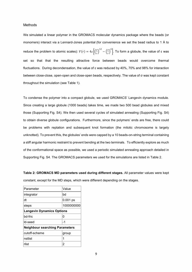
Table 2: GROMACS MD parameters used during different stages. All parameter values were kept

constant, except for the MD steps, which were different depending on the stages.

Parameter Value integrator bd dt 0.001 ps steps 1000000000 Langevin Dynamics Options bd-fric 0 ld-seed -1 Neighbour searching Parameters cutoff-scheme group nstlist 1 rlist 2

10

Options for van der Waals vdw-type Cut-off rvdw 2 nm Temperature coupling Tcoupl v-rescale nsttcouple 1 tau_t 0.001 ps ref_t 200K

The above simulation protocol leads to a spherically shaped object. However, the mitotic chromosome

is elongated rather than spherical. To achieve this, we used so-called steered MD simulation with zero

pulling velocity. Simply put, we introduced a harmonic pull potential between the centre of masses

between the two 500 bead globules while they mixed. After globule formation, we let the globule unfold

under thermal fluctuations. In the flexible regions (red beads) we lower the Lennard-Jones parameters

compared to the compact region (grey). We show these and all other GROMACS force-field parameters

in Table 1 and Table 2.

References

Antonin W, Neumann H (2016) Chromosome condensation and decondensation during mitosis Curr Opin Cell Biol 40:15-22 doi:10.1016/j.ceb.2016.01.013

Barbieri M, Chotalia M, Fraser J, Lavitas LM, Dostie J, Pombo A, Nicodemi M (2012) Complexity of chromatin folding is captured by the strings and binders switch model Proc Natl Acad Sci U S A 109:16173-16178 doi:10.1073/pnas.1204799109

Belmont AS (2006) Mitotic chromosome structure and condensation Curr Opin Cell Biol 18:632-638 doi:10.1016/j.ceb.2006.09.007

Cremer T, Cremer C (2001) Chromosome territories, nuclear architecture and gene regulation in mammalian cells Nat Rev Genet 2:292-301 doi:10.1038/35066075

Dekker J, Marti-Renom MA, Mirny LA (2013) Exploring the three-dimensional organization of genomes: interpreting chromatin interaction data Nat Rev Genet 14:390-403 doi:10.1038/nrg3454

Dixon JR et al. (2012) Topological domains in mammalian genomes identified by analysis of chromatin interactions Nature 485:376-380 doi:10.1038/nature11082

Fraser J et al. (2015) Hierarchical folding and reorganization of chromosomes are linked to transcriptional changes in cellular differentiation Mol Syst Biol 11:852 doi:10.15252/msb.20156492

Fraser J, Rousseau M, Shenker S, Ferraiuolo MA, Hayashizaki Y, Blanchette M, Dostie J (2009) Chromatin conformation signatures of cellular differentiation Genome Biol 10:R37 doi:10.1186/gb-2009-10-4-r37

Fullwood MJ et al. (2009) An oestrogen-receptor-alpha-bound human chromatin interactome Nature 462:58-64 doi:10.1038/nature08497

11

Gondor A (2013) Dynamic chromatin loops bridge health and disease in the nuclear landscape Semin Cancer Biol 23:90-98 doi:10.1016/j.semcancer.2013.01.002

Grosberg A, Rabin Y, Havlin S, Neer A (1993) Crumpled Globule Model of the 3-Dimensional Structure of DNA Europhys Lett 23:373-378 doi:Doi 10.1209/0295-5075/23/5/012

Hug CB, Grimaldi AG, Kruse K, Vaquerizas JM (2017) Chromatin Architecture Emerges during Zygotic Genome Activation Independent of Transcription Cell 169:216-228 e219 doi:10.1016/j.cell.2017.03.024

Knight PA, Ruiz D (2013) A fast algorithm for matrix balancing Ima J Numer Anal 33:1029-1047 doi:10.1093/imanum/drs019

Krijger PH, de Laat W (2016) Regulation of disease-associated gene expression in the 3D genome Nat Rev Mol Cell Biol 17:771-782 doi:10.1038/nrm.2016.138

Kumar R, Sobhy H, Stenberg P, Lizana L (2017) Genome contact map explorer: a platform for the comparison, interactive visualization and analysis of genome contact maps Nucleic Acids Res 45:e152 doi:10.1093/nar/gkx644

Li G, Sudlow G, Belmont AS (1998) Interphase cell cycle dynamics of a late-replicating, heterochromatic homogeneously staining region: precise choreography of condensation/decondensation and nuclear positioning J Cell Biol 140:975-989

Lieberman-Aiden E et al. (2009) Comprehensive mapping of long-range interactions reveals folding principles of the human genome Science 326:289-293 doi:10.1126/science.1181369

Maison C, Almouzni G (2004) HP1 and the dynamics of heterochromatin maintenance Nat Rev Mol Cell Biol 5:296-304 doi:10.1038/nrm1355

Mirny LA (2011) The fractal globule as a model of chromatin architecture in the cell Chromosome Res 19:37-51 doi:10.1007/s10577-010-9177-0

Mora-Bermudez F, Gerlich D, Ellenberg J (2007) Maximal chromosome compaction occurs by axial shortening in anaphase and depends on Aurora kinase Nat Cell Biol 9:822-831 doi:10.1038/ncb1606

Naumova N, Imakaev M, Fudenberg G, Zhan Y, Lajoie BR, Mirny LA, Dekker J (2013) Organization of the mitotic chromosome Science 342:948-953 doi:10.1126/science.1236083

Nora EP et al. (2012) Spatial partitioning of the regulatory landscape of the X-inactivation centre Nature 485:381-385 doi:10.1038/nature11049

Rosa A, Zimmer C (2014) Computational models of large-scale genome architecture Int Rev Cell Mol Biol 307:275-349 doi:10.1016/B978-0-12-800046-5.00009-6

Sachs RK, van den Engh G, Trask B, Yokota H, Hearst JE (1995) A random-walk/giant-loop model for interphase chromosomes Proc Natl Acad Sci U S A 92:2710-2714

Sanborn AL et al. (2015) Chromatin extrusion explains key features of loop and domain formation in wild-type and engineered genomes Proc Natl Acad Sci U S A 112:E6456-6465 doi:10.1073/pnas.1518552112

Schneider R, Grosschedl R (2007) Dynamics and interplay of nuclear architecture, genome organization, and gene expression Genes Dev 21:3027-3043 doi:10.1101/gad.1604607

Sexton T, Schober H, Fraser P, Gasser SM (2007) Gene regulation through nuclear organization Nat Struct Mol Biol 14:1049-1055 doi:10.1038/nsmb1324

Therizols P, Duong T, Dujon B, Zimmer C, Fabre E (2010) Chromosome arm length and nuclear constraints determine the dynamic relationship of yeast subtelomeres Proc Natl Acad Sci U S A 107:2025-2030 doi:10.1073/pnas.0914187107

12

Figure S1: Contact map of crumpled globules. Average bead-bead contact map obtained from an

ensemble of crumpled globules.

13

Figure S2: The radius of gyration as a function of epsilon. The black line is based on an average of 10 globule configurations at each epsilon value. In this simulation all beads in the polymer are identical.

14

Figure S3: Volume of the condensed and decondensed state. Volume distribution for realized

configurations of globules at condensed and decondensed states were calculated from the simulations.

To calculate volume of the globules, we considered a probe of 2 Å to create a probe accessible surface

enclosing the globule and calculated volume of this enclosed shape very similar to solvent accessible

surface for macromolecules using the GROMACS tool g_sas. The probe of 2 Å radius was considered

because 4 Å was used to calculate the contact map and with this radius, two beads in contact will be

inside the same enclosed surface when rolling the probe over the globule.

15

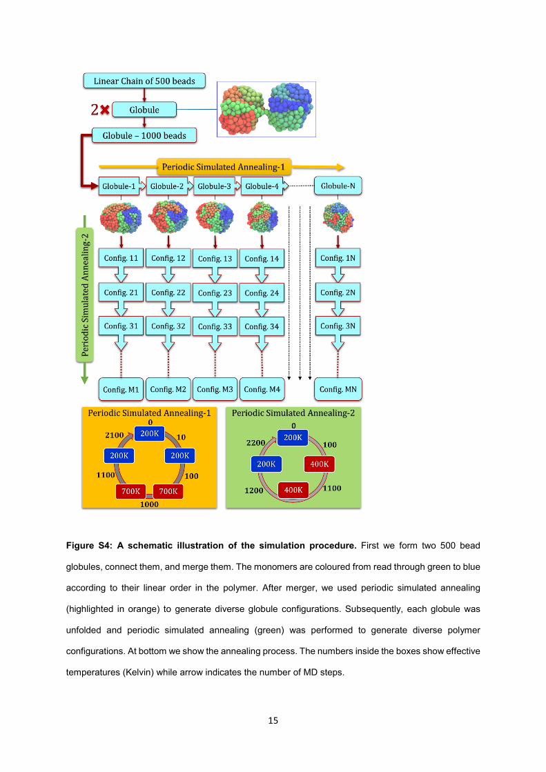
Figure S4: A schematic illustration of the simulation procedure. First we form two 500 bead

globules, connect them, and merge them. The monomers are coloured from read through green to blue

according to their linear order in the polymer. After merger, we used periodic simulated annealing

(highlighted in orange) to generate diverse globule configurations. Subsequently, each globule was

unfolded and periodic simulated annealing (green) was performed to generate diverse polymer

configurations. At bottom we show the annealing process. The numbers inside the boxes show effective

temperatures (Kelvin) while arrow indicates the number of MD steps.