genopz synchronous machine model - genopz synchronous... · of machine modeling presently in use...
TRANSCRIPT

genopz
Synchronous Machine Model
John UndrillAugust 2019

132 CHAPTER 7. SYNCHRONOUS MACHINES
To develop the two transfer functions we must enter the ’culture’ of synchronous machinetheory.
7.4.4 Sudden short circuit
The unidirectional and alternating currents produced by a synchronous machine when thestator winding is short circuited suddenly from an initial condition of rated voltage and opencircuit take the form illustrated by figures 7.4 and 7.5.
The features of the alternating component of short circuit current behavior seen in figures 7.4and 7.5 can be described by the transfer function model given in the following section. The timeconstants in the numerators of the transfer functions are those of the decay of the waveformenvelopes shown in the bottom of figure 7.4 and in figure 7.5. The paramters Ld, L0
d, L”d are thereciprocals of waveform amplitudes as identified in figure 7.5.
7.4.5 Operational Impedances
When a machine is producing reactive power, but no real power, at its terminals its behavior,as can be observed in various tests including a sudden short circuit test, can be describedcompletely emperically by the transfer function relationship
vq(s) = Yd(s) = G(s)Ef d(s)� Ld(s)Id(s) (7.4)
in which
vq is the amplitude of the positive sequence AC voltage at the terminals the machineYd is the amplitude of the flux wave linking the stator windingEf d is the voltage applied to the field windingId is the amplitude of the positive sequence current in the stator winding
The transfer functions have the form
Ld(s) = (Ld � Ll)
0
@1 + (L0
d�Ll)(Ld�Ll)
T0dos
1 + T0dos
1
A
0
@1 + (L”d�Ll)
(L0d�Ll)
T”dos
1 + T”dos
1
A+ Ll (7.5)
G(s) =✓
11 + sT0
do
◆0
@1 + (L”d�Ll)
(L0d�Ll) T”dos
1 + sT”do
1
A (7.6)
Figure 7.6 shows the form of the transfer function, Ld(jw).
The transfer function expression Ld(s) can be written by direct reference to figures 7.4 and 7.5.This transfer function can also be derived from the basic electromagnetic equations describing
168 CHAPTER 7. SYNCHRONOUS MACHINES
7.14 Generator dynamic models for simulations
7.14.1 Initial deveopment of transfer function model
While the synchronous modeling described in section 7.5 is straightforward and can accommodatecomprehensive treatment of magnetic saturation it is not used directly in the large scale dynamicsimulation programs presently in widespread use. Among the reasons for this:
The early development of electric machine modeling preceded the development of digitalcomputers and calculations that are routine today were impractical with the tools thenavailable; approximations and simplifications were essential. Many of the implementationsof machine modeling presently in use owe their form to such simplifications.
The inductance coefficients appearing in equations (7.7)-(7.17) are not readily availableand do not directly describe characteristics of the machine that can be measured in tests.
The long-established tests of synchronous machines yield values of the parameters appearingin the operational impedance, equation (7.5). The modeling used in production simulationassumes that the following parameters are available for the direct and quadrature axes:
L synchronous reactanceL0 transient reactanceL” subtransient reactanceT0 transient open circuit time constantT” subtransient open circuit time constant
Construction of a transfer function starts with breaking the operational impedance (7.5) into itspartial fractions. We use a and b to represent the ratios as follows:
a = (L0 � Ll)/(L � Ll)b = (L” � Ll)/(L0 � Ll)
Then (7.5) can be written as
L(s) =(L � Ll)(1 + saTa)(1 + sbTb)
(1 + sTa)(1 + sTb)+ Ll (7.80)
and the partial fraction expansion proceeds to yield
L(s) = (L � Ll)
✓a +
1 � a1 + sTa
◆✓b +
1 � b1 + sTb
◆+ Ll (7.81)
L(s) = (L � Ll)
✓ab +
(1 � a)b1 + sTa
+a(1 � b)1 + sTb
+(1 � a)(1 � b)
(1 + sTa)(1 + sTb)
◆+ Ll (7.82)

Ld(s) = (Ld − Ll)
⎛
⎝
(
1 +(L′
d−Ll)
(Ld−Ll)T ′
dos
)(
1 + (L”d−Ll)(L′
d−Ll)
T”dos)
(1 + T ′
dos)(1 + T”dos)
⎞
⎠+ Ll
G(s) =1 + L”d−Ll)
(L′
d−Ll)T”dos
(1 + sT ′
do)(1 + sT”do)
Current interruption test reveals generator d-axis characteristics
7.13. SUDDEN SHORT CIRCUIT TEST 167
We now have the generator equations, for the special case of a simple impedance load, in thestandard form
dyrdt
= Ayr (7.79)
The dynamic behavior of the generator in a short circuit is defined by the eigenvalues of thematrix A, with the note that analysis by the direct use of A will be an approximation to theextent that it ignores the variation of generator inductances due to magnetic saturation.
(a)Initial
0.9 0.95 1 1.05 1.1 1.15 1.2 1.25 1.3 1.35 1.40
0.5
1
1.5
2
2.5
3
3.5
4
4.5
5
Time, sec
(b)Full
0 1 2 3 4 5 6 7 8 9 100
0.5
1
1.5
2
2.5
3
3.5
4
4.5
5
Time, sec
Figure 7.33: Simulation of three phase sudden short circuit - direct axis variablesRed - stator current
Blue - field winding currentMagenta - Iron circuit current
Black - terminal voltage
Figure 7.33 shows the result of using the differential equation (7.77) to simulate the behaviorof a generator when subjected to a three phase short circuit, from an initially open circuittest condition. The stator current (red) has the expected form of an initial rapid decay, amuch slower decay, and a final steady value. The rotor currents (blue, magenta) are seento be associated with the variation of the stator current. At the moment the fault is appliedthe currents in the field winding (blue) and iron circuit (magenta) jump to positive values toprovide the magnetomotive force needed to maintain the flux linkages in the rotor circuits.Then the current in the iron circuit, whose resistance is relatively high, decays rapidly. As themmf provided by the ’iron’ current disappears the current in the field winding increases tomake up for the quick loss of mmf. Note that current, small but not zero, continues to flowin the iron circuit as long as stator and field winding currents are changing. At the end of thetransient the field current has returned to its original value and the current in the iron circuithas returned to zero.

Ld(s) = (Ld − Ll)
⎛
⎝
(
1 +(L′
d−Ll)
(Ld−Ll)T ′
dos
)(
1 + (L”d−Ll)(L′
d−Ll)
T”dos)
(1 + T ′
dos)(1 + T”dos)
⎞
⎠+ Ll
G(s) =1 + L”d−Ll)
(L′
d−Ll)T”dos
(1 + sT ′
do)(1 + sT”do)
Current interruption test reveals generator d-axis characteristics

7.14. GENERATOR DYNAMIC MODELS FOR SIMULATIONS 169
Similar partial fraction expansion can be used for the transfer function, G(s), in equation (7.6)to yield.
G(s) =✓
b1 + sTa
+(1 � b)
(1 + sTa)(1 + sTb)
◆(7.83)
Then a transfer function diagram implementing equations (7.4), (7.5), and (7.6) with the partialfraction relationships can be drawn ’by inspection’. One possible form is shown in figure 7.34.
Figure 7.34: Transfer function block diagram corresponding to partial-fraction expression (7.83).
In the absence of saturation the abbreviations, a and b in the figure represent constants; recognitionof saturation makes them variables that must be reevaluated at each step of a numerical integrationprocess.
Expanding the expressions involving a and b in figure 7.34 results in figure 7.35.
Figure 7.35: Transfer function block diagram 7.34 with expressions in a, b expanded.
It should be noted that the development of figures 7.34 and 7.35 is completely emperical;it requires no knowledge of internal details of the machine, only values describing featuresobserved in test results. This point is important in commerce because specifications of machineryshould, wherever possible, be stated in terms of characteristics that can be measured directlyin normal operation or in practical tests.
168 CHAPTER 7. SYNCHRONOUS MACHINES
7.14 Generator dynamic models for simulations
7.14.1 Initial deveopment of transfer function model
While the synchronous modeling described in section 7.5 is straightforward and can accommodatecomprehensive treatment of magnetic saturation it is not used directly in the large scale dynamicsimulation programs presently in widespread use. Among the reasons for this:
The early development of electric machine modeling preceded the development of digitalcomputers and calculations that are routine today were impractical with the tools thenavailable; approximations and simplifications were essential. Many of the implementationsof machine modeling presently in use owe their form to such simplifications.
The inductance coefficients appearing in equations (7.7)-(7.17) are not readily availableand do not directly describe characteristics of the machine that can be measured in tests.
The long-established tests of synchronous machines yield values of the parameters appearingin the operational impedance, equation (7.5). The modeling used in production simulationassumes that the following parameters are available for the direct and quadrature axes:
L synchronous reactanceL0 transient reactanceL” subtransient reactanceT0 transient open circuit time constantT” subtransient open circuit time constant
Construction of a transfer function starts with breaking the operational impedance (7.5) into itspartial fractions. We use a and b to represent the ratios as follows:
a = (L0 � Ll)/(L � Ll)b = (L” � Ll)/(L0 � Ll)
Then (7.5) can be written as
L(s) =(L � Ll)(1 + saTa)(1 + sbTb)
(1 + sTa)(1 + sTb)+ Ll (7.80)
and the partial fraction expansion proceeds to yield
L(s) = (L � Ll)
✓a +
1 � a1 + sTa
◆✓b +
1 � b1 + sTb
◆+ Ll (7.81)
L(s) = (L � Ll)
✓ab +
(1 � a)b1 + sTa
+a(1 � b)1 + sTb
+(1 � a)(1 � b)
(1 + sTa)(1 + sTb)
◆+ Ll (7.82)

Red genrouGreen gentpjBlue genopz
ci-man.pdf
CurrentInterruption
Constant Efd
ci-auto.pdf
Red genrouGreen gentpjBlue genopz
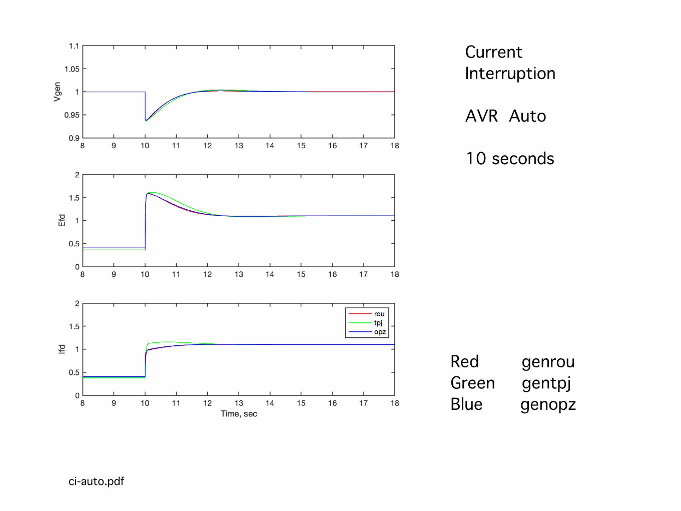
CurrentInterruption
AVR Auto
10 seconds

ci-auto-s.pdf
Red genrouGreen gentpjBlue genopz
CurrentInterruption
AVR Auto
1 second

avrstep-offline.pdf
Red genrouGreen gentpjBlue genopz
AVR referencestep
Off line

avrstep-online.pdf
Red genrouGreen gentpjBlue genopz
AVR referencestep
On line

Ld(s) = (Ld − Ll)
⎛
⎝
1 +(L′
d−Ll)
(Ld−Ll)T ′
dos
1 + T ′
dos
⎞
⎠
⎛
⎝
1 + (L”d−Ll)(L′
d−Ll)
T”dos
1 + T”dos
⎞
⎠+ Ll
L(s) = (L− Ll)
(
ab+(1− a)b
1 + sTa
+a(1− b)
1 + sTb
+(1− a)(1− b)
(1 + sTa)(1 + sTb)
)
+ Ll

gopz dynamic model
Same saturation treatment as gentpj
Saturation is a function of BOTH air gap flux and stator current
Does not depend on assumed relationships among inductance coefficients
Is readily related to basic observable performance characteristics
Is simple to explain

Notes on generator models
ALL of our generator models are approximationswith regard to
magnetic saturationtorque developed during transmission faults. . . . . .
Which one of our models is best suited for any particular application is dependent on
the electrical configuration in questionthe disturbance under considerationthe time frame of the post disturbance event
Continued evolution of generator models is to beencouraged