RESEARCH ARTICLE10.1002/2014GC005469

Modeling ash fall distribution from a YellowstonesupereruptionLarry G. Mastin1, Alexa R. Van Eaton2, and Jacob B. Lowenstern3

1U.S. Geological Survey, Cascades Volcano Observatory, Vancouver, Washington, USA, 2School of Earth and SpaceExploration, Arizona State University, Tempe, Arizona, USA, 3U.S. Geological Survey, Yellowstone Volcano Observatory,Menlo Park, California, USA

Abstract We used the volcanic ash transport and dispersion model Ash3d to estimate the distribution ofashfall that would result from a modern-day Plinian supereruption at Yellowstone volcano. The simulationsrequired modifying Ash3d to consider growth of a continent-scale umbrella cloud and its interaction withambient wind fields. We simulated eruptions lasting 3 days, 1 week, and 1 month, each producing 330 km3

of volcanic ash, dense-rock equivalent (DRE). Results demonstrate that radial expansion of the umbrellacloud is capable of driving ash upwind (westward) and crosswind (N-S) in excess of 1500 km, producingmore-or-less radially symmetric isopachs that are only secondarily modified by ambient wind. Deposit thick-nesses are decimeters to meters in the northern Rocky Mountains, centimeters to decimeters in the north-ern Midwest, and millimeters to centimeters on the East, West, and Gulf Coasts. Umbrella cloud growth mayexplain the extremely widespread dispersal of the �640 ka and 2.1 Ma Yellowstone tephra deposits in theeastern Pacific, northeastern California, southern California, and South Texas.

1. Introduction

The consequences of a future, caldera-forming eruption from Yellowstone have been the subject of muchspeculation but little quantitative research in terms of regional ashfall impacts. Despite graphic and oftenfanciful media depictions of the devastation and the impact on human life that would result from a modernsupereruption (producing >1000 km3 volcanic ash or >400 km3 DRE of magma), no historical examplesexist from which to draw comparison [Self, 2006]. The largest eruptions of the past few centuries have pro-duced a few to several tens of cubic kilometers of magma. Examples include Tambora volcano, Indonesia in1815 [Oppenheimer, 2003], Krakatau in 1883 [Simkin and Fiske, 1983], the Katmai/Valley of Ten ThousandSmokes eruption, Alaska in 1912 [Hildreth, 1983], Quizapu volcano, Chile in 1932 [Hildreth and Drake, 1992],and most recently, Pinatubo, Philippines in 1991 [Newhall and Punongbayan, 1996]. These erupted volumesare much larger than the Mount St. Helens eruption in 1980 (0.2–0.4 km3) [Pallister et al., 1992], but at leastan order of magnitude smaller than the largest Yellowstone events [Christiansen and Blank, 1972].

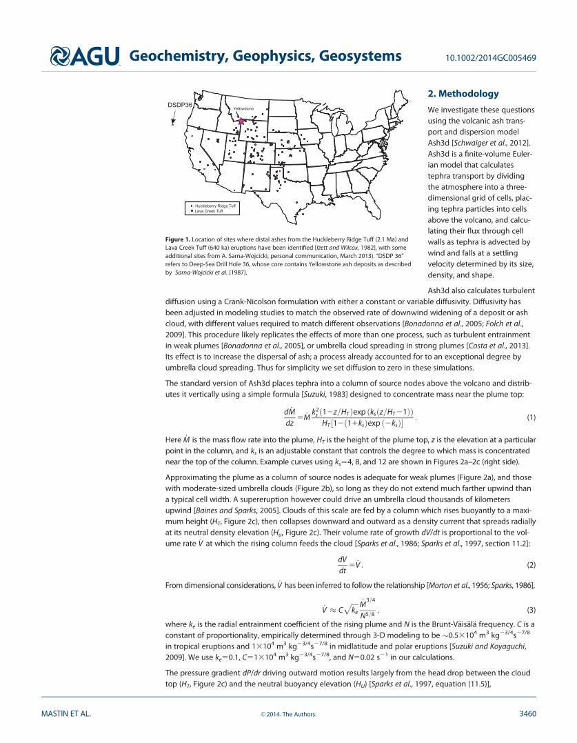
From geological evidence, we know that ash from the last large eruptions at Yellowstone (2.1 Ma, 1.3 Ma,and 640 ka) spread over many tens of thousands of square kilometers. These tephra deposits howeverhave been remobilized in the millennia after emplacement, and estimates of primary ash thickness arechallenging to obtain. Widespread Yellowstone-derived deposits, known as the ‘‘Pearlette ash beds,’’ havebeen important stratigraphic markers throughout the central and western United States and Canada(Figure 1), even before their volcanic source location was recognized [Wilcox and Naeser, 1992]. Izett andWilcox [1982] listed nearly 300 locations for Yellowstone ashes spread as widely as California, Texas, Iowaand Saskatchewan. Over 3 m of ash from the Lava Creek Tuff eruption (640 ka) are found in north-centralTexas. In the Gulf of Mexico, tens of meters of ash-dominated deposits were emplaced immediately fol-lowing the 2.1 Ma Huckleberry Ridge Tuff eruption [Dobson et al., 1991] and the later Lava Creek eruption.The great thickness of these and other deposits [Izett and Wilcox, 1982] partially reflects fluvial and (or)aeolian reworking, obscuring the primary distribution of ash thicknesses. In this study, we address the fol-lowing questions: (1) given modern meteorological patterns, where and how much ash would be depos-ited by a Yellowstone supereruption? (2) how sensitive is the thickness distribution to changes in theseason and duration of eruptive pulses? and (3) what is the long-term (probabilistic) estimate of ashfalldistribution?

Key Points:� We model tephra fall from a

Yellowstone supereruption� Growth of an umbrella cloud was

considered� Umbrella cloud may drive ash>1500km upwind

Supporting Information:� Readme� Simulation results� Wind data

Correspondence to:L. G. Mastin,lgmastin@usgs.gov

Citation:Mastin, L. G., A. R. Van Eaton, andJ. B. Lowenstern (2014), Modeling ashfall distribution from a Yellowstonesupereruption, Geochem. Geophys.Geosyst., 15, 3459–3475, doi:10.1002/2014GC005469.

Received 26 JUN 2014

Accepted 28 JUL 2014

Published online 27 AUG 2014

This is an open access article under the

terms of the Creative Commons

Attribution-NonCommercial-NoDerivs

License, which permits use and

distribution in any medium, provided

the original work is properly cited, the

use is non-commercial and no

modifications or adaptations are

made.

MASTIN ET AL. VC 2014. The Authors. 3459

Geochemistry, Geophysics, Geosystems

PUBLICATIONS

2. Methodology

We investigate these questionsusing the volcanic ash trans-port and dispersion modelAsh3d [Schwaiger et al., 2012].Ash3d is a finite-volume Euler-ian model that calculatestephra transport by dividingthe atmosphere into a three-dimensional grid of cells, plac-ing tephra particles into cellsabove the volcano, and calcu-lating their flux through cellwalls as tephra is advected bywind and falls at a settlingvelocity determined by its size,density, and shape.

Ash3d also calculates turbulentdiffusion using a Crank-Nicolson formulation with either a constant or variable diffusivity. Diffusivity hasbeen adjusted in modeling studies to match the observed rate of downwind widening of a deposit or ashcloud, with different values required to match different observations [Bonadonna et al., 2005; Folch et al.,2009]. This procedure likely replicates the effects of more than one process, such as turbulent entrainmentin weak plumes [Bonadonna et al., 2005], or umbrella cloud spreading in strong plumes [Costa et al., 2013].Its effect is to increase the dispersal of ash; a process already accounted for to an exceptional degree byumbrella cloud spreading. Thus for simplicity we set diffusion to zero in these simulations.

The standard version of Ash3d places tephra into a column of source nodes above the volcano and distrib-utes it vertically using a simple formula [Suzuki, 1983] designed to concentrate mass near the plume top:

d _Mdz

5 _Mk2

s 12z=HTð Þexp ks z=HT 21ð Þð ÞHT 12 11ksð Þexp 2ksð Þ½ � : (1)

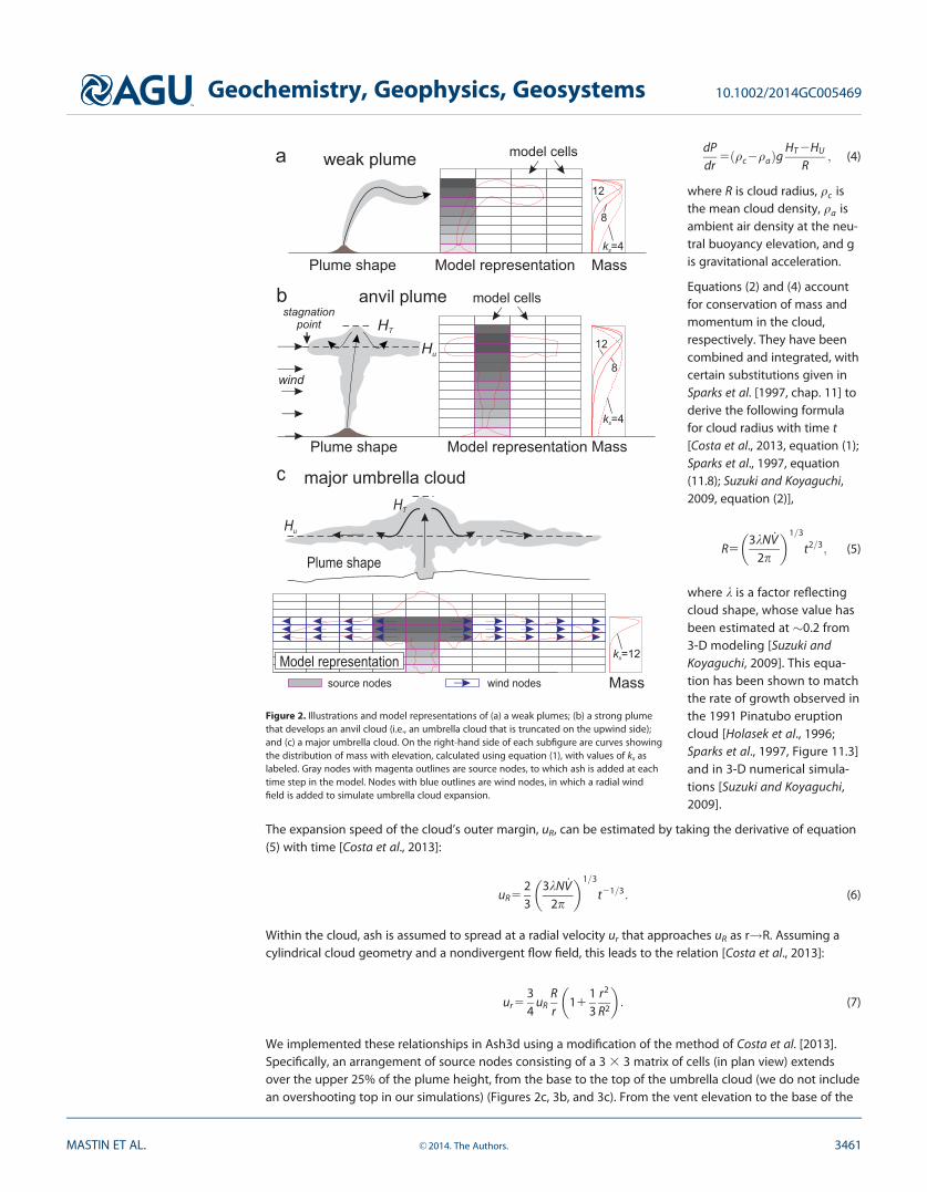
Here _M is the mass flow rate into the plume, HT is the height of the plume top, z is the elevation at a particularpoint in the column, and ks is an adjustable constant that controls the degree to which mass is concentratednear the top of the column. Example curves using ks54, 8, and 12 are shown in Figures 2a–2c (right side).

Approximating the plume as a column of source nodes is adequate for weak plumes (Figure 2a), and thosewith moderate-sized umbrella clouds (Figure 2b), so long as they do not extend much farther upwind thana typical cell width. A supereruption however could drive an umbrella cloud thousands of kilometersupwind [Baines and Sparks, 2005]. Clouds of this scale are fed by a column which rises buoyantly to a maxi-mum height (HT, Figure 2c), then collapses downward and outward as a density current that spreads radiallyat its neutral density elevation (Hu, Figure 2c). Their volume rate of growth dV/dt is proportional to the vol-ume rate _V at which the rising column feeds the cloud [Sparks et al., 1986; Sparks et al., 1997, section 11.2]:

dVdt

5 _V : (2)

From dimensional considerations, _V has been inferred to follow the relationship [Morton et al., 1956; Sparks, 1986],

_V � Cffiffiffiffike

p _M3=4

N5=8; (3)

where ke is the radial entrainment coefficient of the rising plume and N is the Brunt-V€ais€al€a frequency. C is aconstant of proportionality, empirically determined through 3-D modeling to be �0.53104 m3 kg23/4s27/8

in tropical eruptions and 13104 m3 kg23/4s27/8 in midlatitude and polar eruptions [Suzuki and Koyaguchi,2009]. We use ke50.1, C513104 m3 kg23/4s27/8, and N50.02 s21 in our calculations.

The pressure gradient dP/dr driving outward motion results largely from the head drop between the cloudtop (HT, Figure 2c) and the neutral buoyancy elevation (HU) [Sparks et al., 1997, equation (11.5)],

Huckleberry Ridge TuffLava Creek Tuff

YellowstoneDSDP36

Figure 1. Location of sites where distal ashes from the Huckleberry Ridge Tuff (2.1 Ma) andLava Creek Tuff (640 ka) eruptions have been identified [Izett and Wilcox, 1982], with someadditional sites from A. Sarna-Wojcicki, personal communication, March 2013). ‘‘DSDP 36’’refers to Deep-Sea Drill Hole 36, whose core contains Yellowstone ash deposits as describedby Sarna-Wojcicki et al. [1987].

Geochemistry, Geophysics, Geosystems 10.1002/2014GC005469

MASTIN ET AL. VC 2014. The Authors. 3460

dPdr

5 qc2qað Þg HT 2HU

R; (4)

where R is cloud radius, qc isthe mean cloud density, qa isambient air density at the neu-tral buoyancy elevation, and gis gravitational acceleration.

Equations (2) and (4) accountfor conservation of mass andmomentum in the cloud,respectively. They have beencombined and integrated, withcertain substitutions given inSparks et al. [1997, chap. 11] toderive the following formulafor cloud radius with time t[Costa et al., 2013, equation (1);Sparks et al., 1997, equation(11.8); Suzuki and Koyaguchi,2009, equation (2)],

R53kN _V

2p

� �1=3

t2=3; (5)

where k is a factor reflectingcloud shape, whose value hasbeen estimated at �0.2 from3-D modeling [Suzuki andKoyaguchi, 2009]. This equa-tion has been shown to matchthe rate of growth observed inthe 1991 Pinatubo eruptioncloud [Holasek et al., 1996;Sparks et al., 1997, Figure 11.3]and in 3-D numerical simula-tions [Suzuki and Koyaguchi,2009].

The expansion speed of the cloud’s outer margin, uR, can be estimated by taking the derivative of equation(5) with time [Costa et al., 2013]:

uR523

3kN _V2p

� �1=3

t21=3: (6)

Within the cloud, ash is assumed to spread at a radial velocity ur that approaches uR as r!R. Assuming acylindrical cloud geometry and a nondivergent flow field, this leads to the relation [Costa et al., 2013]:

ur534

uRRr

1113

r2

R2

� �: (7)

We implemented these relationships in Ash3d using a modification of the method of Costa et al. [2013].Specifically, an arrangement of source nodes consisting of a 3 3 3 matrix of cells (in plan view) extendsover the upper 25% of the plume height, from the base to the top of the umbrella cloud (we do not includean overshooting top in our simulations) (Figures 2c, 3b, and 3c). From the vent elevation to the base of the

b

a

c

wind

weak plume

anvil plume

major umbrella cloud

stagnation point

Hu

HT

HT

Plume shape

Plume shape

Plume shape

Model representation

Model representation

Hu

source nodes wind nodes

Model representation

model cells

model cells

k =4s

k =4s

k =12s

8

8

12

12

Mass

Mass

Mass

Figure 2. Illustrations and model representations of (a) a weak plumes; (b) a strong plumethat develops an anvil cloud (i.e., an umbrella cloud that is truncated on the upwind side);and (c) a major umbrella cloud. On the right-hand side of each subfigure are curves showingthe distribution of mass with elevation, calculated using equation (1), with values of ks aslabeled. Gray nodes with magenta outlines are source nodes, to which ash is added at eachtime step in the model. Nodes with blue outlines are wind nodes, in which a radial windfield is added to simulate umbrella cloud expansion.

Geochemistry, Geophysics, Geosystems 10.1002/2014GC005469

MASTIN ET AL. VC 2014. The Authors. 3461

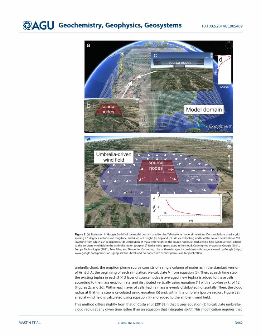
umbrella cloud, the eruption plume source consists of a single column of nodes as in the standard versionof Ash3d. At the beginning of each simulation, we calculate _V from equation (3). Then, at each time step,the existing tephra in each 3 3 3 layer of source nodes is averaged; new tephra is added to these cellsaccording to the mass eruption rate, and distributed vertically using equation (1) with a top-heavy ks of 12(Figures 2c and 3d). Within each layer of cells, tephra mass is evenly distributed horizontally. Then, the cloudradius at that time step is calculated using equation (5) and, within the umbrella (purple region, Figure 3e),a radial wind field is calculated using equation (7) and added to the ambient wind field.

This method differs slightly from that of Costa et al. [2013] in that it uses equation (5) to calculate umbrella-cloud radius at any given time rather than an equation that integrates dR/dt. This modification requires that

YellowstoneLake

ac

source nodes

b sourcenodes

e

sourcenodes

Umbrella-drivenwind field

Mass

Hei

ght

d

0 10

4

8

r/R

u/u r

R

uR

R

f

Model domain

Figure 3. (a) Illustration in Google EarthVR of the model domain used for the Yellowstone model simulations. Our simulations used a gridspacing 0.5 degrees latitude and longitude, and 4 km cell height. (b) Top and (c) side view (looking north) of the source nodes above Yel-lowstone from which ash is dispersed. (d) Distribution of mass with height in the source nodes. (e) Radial wind field (white arrows) addedto the ambient wind field in the umbrella region (purple). (f) Radial wind speed ur/uR in the cloud. Copyrighted images by Google (2011),Europa Technologies (2011), Tele Atlas, and Geocenter Consulting. Use of these images is consistent with usage allowed by Google (http://www.google.com/permissions/geoguidelines.html) and do not require explicit permission for publication.

Geochemistry, Geophysics, Geosystems 10.1002/2014GC005469

MASTIN ET AL. VC 2014. The Authors. 3462

the eruption be specified as a single pulse of con-stant plume height and eruption rate rather than atime series of heights and rates.

The appendix A provides a validation of thisapproach by comparing Ash3d simulations to thewell-documented growth of the 1991 Pinatuboumbrella cloud. Ash3d does not resolve thedynamics of eruption plume ascent – instead, theheight and vertical distribution of mass are heldconstant throughout the eruption. Despite ahighly parameterized depiction of the plume, themodel’s key strength is its ability to examine thelong-distance umbrella expansion and dispersal oferupted material in a complex, time-varying windfield.

3. Model inputs

Inputs to the model include a 3-D time-varyingmeteorological wind field; volume of magmaerupted; eruption start time; eruption duration;column height; and the size, density, and shapefactor of erupted fragments. Our choice of inputsis described below.

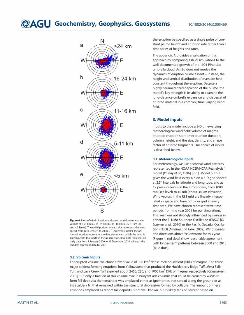
3.1. Meteorological InputsFor meteorology, we use historical wind patternsrepresented in the NOAA NCEP/NCAR Reanalysis 1model [Kalnay et al., 1996] (RE1). Model outputgives the wind field every 6 h on a 3-D grid spacedat 2.5� intervals in latitude and longitude, and at17 pressure levels in the atmosphere, from 1000mb (sea level) to 10 mb (about 34 km elevation).Wind vectors in the RE1 grid are linearly interpo-lated in space and time onto our grid at everytime step. We have chosen representative timeperiods from the year 2001 for our simulations.This year was not strongly influenced by swings ineither the El Ni~no Southern Oscillation (ENSO) [DiLorenzo et al., 2010] or the Pacific Decadal Oscilla-tion (PDO) [Mantua and Hare, 2002]. Wind speedsand directions above Yellowstone for this year(Figure 4, red dots) show reasonable agreementwith longer-term patterns between 2000 and 2010(blue dots).

3.2. Volcanic InputsFor erupted volume, we chose a fixed value of 330 km3 dense-rock equivalent (DRE) of magma. The threemajor caldera-forming eruptions from Yellowstone that produced the Huckleberry Ridge Tuff, Mesa FallsTuff, and Lava Creek Tuff expelled about 2450, 280, and 1000 km3 DRE of magma, respectively [Christiansen,2001]. But only a fraction of this volume rose in buoyant ash columns that could be carried by winds toform fall deposits; the remainder was emplaced either as ignimbrites that spread along the ground or asintracaldera fill that remained within the structural depression formed by collapse. The amount of theseeruptions emplaced as tephra fall deposits is not well known, but is likely tens of percent based on

<5 km

5-11 km

11-16 km

16-24 km

>24 kma

b

c

d

e

N

S

W E

E

E

E

E

W

W

W

W

Figure 4. Plots of wind direction and speed at Yellowstone at ele-vations of >24 km (a), 16–24 km (b), 11–16 km (c), 5–11 km (d),and <5 km (e). The radial position of each dot represents the windspeed, from zero (center) to 70 m s21 (outermost circle); the azi-muthal location represents the direction toward which the wind isblowing, with true north in the up direction. Blue dots represent alldaily data from 1 January 2000 to 31 December 2010, whereas thered dots represent data for 2001.

Geochemistry, Geophysics, Geosystems 10.1002/2014GC005469

MASTIN ET AL. VC 2014. The Authors. 3463

better-studied, recent caldera-forming eruptions[e.g., Bacon, 1983; Wilson, 2001, 2008]. For our modelsimulations, the 330 km3 volume represents aboutone to two thirds of the total volume of a 500–1000 km3 eruption, which is above the threshold fora supereruption (1000 km3 bulk or �400 km3 DRE)[Sparks et al., 2005]. Expulsion of 330 km3 DRE ofmagma in a week would imply a mass eruptionrate of 73108 kg s21, assuming a magma densityof 2500 kg m23. This is comparable to the

�3–103108 kg s21 estimated for Pinatubo [Holasek et al., 1996; Koyaguchi and Ohno, 2001; Suzuki andKoyaguchi, 2009].

For eruption duration, we explore values from days to a month, reflecting durations that have been inferredand observed for moderate to large eruptions. The 1912 Novarupta eruption in Alaska, the largest volcaniceruption of the 20th century, ejected 15 km3 of magma over about 52 h [Hildreth, 1983]. The Tambora erup-tion of 1815, the largest in recent centuries, ejected about 50 km3 in 24 h [Self et al., 1984]. The climacticphase of the 1883 Krakatau eruption ejected 10 km3 of magma in about 36 h [Simkin and Fiske, 1983]. Fieldevidence from deposits of the 0.76 Ma Bishop Tuff from the Long Valley Caldera in California suggest that�700 km3 magma was emplaced in a matter of days [Wilson and Hildreth, 1997]. On the other hand, Wilson[2008] estimates that the �26 ka Oruanui eruption was a series of large-scale outbreaks of increasing vigor,including multiple hiatuses of up to several weeks. Many smaller eruptions have persisted for weeks oreven months. Eyjafjallaj€okull volcano in Iceland, whose eruption shut down air space over Europe in Apriland May of 2010, erupted about 0.2 km3 magma in 59 days [Gudmundsson et al., 2012].

For the height of ash injection, several factors are considered. Plume height is known to correlate with erup-tion rate, suggesting that a high-flux Yellowstone eruption would produce a very high plume. But such cor-relations [e.g., Mastin et al., 2009, equation (1); Sparks et al., 1997, equation (5.1)] are based mainly onplumes that emanate from single, central vents, whereas a large, complex Yellowstone plume is more likelyto rise from multiple vents, or as an elutriated ash cloud from pyroclastic flows. The 15 June, 1991 eruptionof Pinatubo produce the highest historically observed plume of �40 km [Holasek et al., 1996], but itsumbrella cloud spread at much lower heights of about 18–25 km [Fero et al., 2009; Holasek et al., 1996;Suzuki and Koyaguchi, 2009]. Based on these observations, most of our simulations use an umbrella cloudwhose top is at 25 km. We also explore end-member values of 15 km and 35 km.

For a particle-size distribution, we run most simulations using values listed in Table 1, referred to as GSD1.The size distribution primarily determines how the deposit is distributed with distance from the vent, with

coarse particles settling nearthe vent and fine particlessettling at greater distance.Ash3d calculates the settlingrate of individual particles ofellipsoidal shape using rela-tions of Wilson and Huang[1979], and a shape factor F(F5(b1c)/2a, where a, b, andc are the semimajor, interme-diate, and semiminor axes ofthe ellipsoid, that is the aver-age of tephra particles meas-ured by Wilson and Huang[1979]. In real eruptions, par-ticles smaller than about0.063 to 0.125 mm aggregateinto clusters and fall outfaster than they would as

Table 1. Grain-Size Distribution GSD1, Used in Most ModelSimulations

Size (mm) Mass Fraction Density (kg/m3)

2 0.25 8001 0.15 8000.5 0.20 10000.25 0.15 10000.125 0.20 18000.0625 0.05 2000

Table 2. Grain-Size Distributions GSD2 and GSD3

Size(mm)

GSD2 ModerateAggregation

MassFraction

GSD3 WeakAggregation

MassFraction

Density(kg/m3)

Individual particles 1 0.043 0.043 19550.707 0.021 0.021 22090.5 0.046 0.046 26120.354 0.072 0.072 26340.25 0.053 0.053 26240.177 0.029 0.029 26900.125 0 0.033 26640.088 0 0.046 26970.063 0 0.060 26980.044 0 0.070 26400.031 0 0.060 25810.022 0 0.021 2570

Aggregate classesfor GSD2

0.297 0.184 0 6000.250 0.184 0 6000.210 0.184 0 6000.177 0.184 0 600

Aggregate classfor GSD3

0.200 0 0.445 200

Geochemistry, Geophysics, Geosystems 10.1002/2014GC005469

MASTIN ET AL. VC 2014. The Authors. 3464

individual particles [Van Eatonet al., 2012]. The physics gov-erning the rate of aggregationis an area of active researchand not yet explicitly resolvedby Ash3d.

To account for these effects,however, we consider a rangeof grain size distributions (GSD)that have been adjusted tomatch observed deposits.GSD1 has been adjusted toreproduce a heavily aggre-gated deposit—the 23 March2009 (event 5) eruption ofRedoubt Volcano, Alaska [Mas-tin et al., 2013b]. This eruptionwas small (�1.6 M m3 DRE)[Wallace et al., 2013] and mixedwith abundant external waterfrom a crater-filling glacier,resulting in extensive ash

aggregation (A.R. Van Eaton et al., unpublished manuscript, 2014). Although a modern Yellowstone eruptionmay interact with external water (e.g., the 350 km2 Yellowstone Lake) magma-water ratios would likely behigher than in the 2009 Redoubt eruption. Therefore, we consider two size distributions that represent lessaggregation. The moderately aggregated GSD2 (Table 2) uses a modification of the total grain-size distribu-tion (TGSD) of the 18 May 1980 Mount St. Helens deposit estimated by Durant et al. [2009, supporting infor-mation file 2008jb005756-txts03.txt], which integrated the deposit to a downwind distance of 671 km. Tosimplify calculations, we consolidated all tephra coarser than 1 mm into a single 1 mm size class. We thensimulate aggregation by moving ash �0.125 mm diameter into four aggregate classes of size 0.177, 0.210,0.250, and 0.297 mm with density 600 kg m23, comparable to ash aggregates of low to intermediate den-sity [Van Eaton et al., 2012]. This scheme can reproduce the 18 May 1980 Mount St. Helens tephra fall distri-bution in Ash3d simulations [Mastin et al., 2013a], and is reasonably consistent with field observations bySorem [1982] that much of the very fine ash fell as clusters 0.25–0.5 mm diameter in the distal area. Theweakly aggregated GSD3 (Table 2) starts with the Mount St. Helens TGSD of Durant et al. [2009], consoli-dates the coarser particles as above, and then moves 25% of the 0.031 mm particles, 75% of the 0.022 mmparticles, and all particles smaller than 0.022 mm into a single aggregate class of 0.20 mm size and a densityof 200 kg m23. Cornell et al. [1983] used this scheme to reproduce 38 ka Campanian Y-5 tephra at CampiFlegrei, Italy, a deposit of >60–100 km3 volume DRE [Cramp et al., 1989].

4. Results

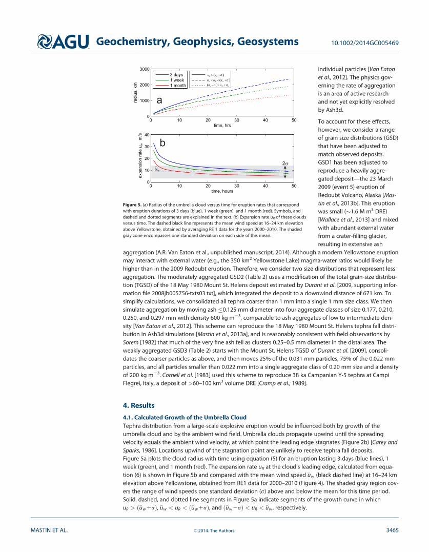
4.1. Calculated Growth of the Umbrella CloudTephra distribution from a large-scale explosive eruption would be influenced both by growth of theumbrella cloud and by the ambient wind field. Umbrella clouds propagate upwind until the spreadingvelocity equals the ambient wind velocity, at which point the leading edge stagnates (Figure 2b) [Carey andSparks, 1986]. Locations upwind of the stagnation point are unlikely to receive tephra fall deposits.Figure 5a plots the cloud radius with time using equation (5) for an eruption lasting 3 days (blue lines), 1week (green), and 1 month (red). The expansion rate uR at the cloud’s leading edge, calculated from equa-tion (6) is shown in Figure 5b and compared with the mean wind speed �uw (black dashed line) at 16–24 kmelevation above Yellowstone, obtained from RE1 data for 2000–2010 (Figure 4). The shaded gray region cov-ers the range of wind speeds one standard deviation (r) above and below the mean for this time period.Solid, dashed, and dotted line segments in Figure 5a indicate segments of the growth curve in whichuR > �uw1rð Þ, �uw < uR < �uw1rð Þ, and �uw2rð Þ < uR < �uw , respectively.

0 10 20 30 40 500

1000

2000

3000

time, hrs

radi

us, k

m

3 days1 week1 month

0 10 20 30 40 500

10

20

30

40

time, hours

expa

nsio

n ra

te u

, m

/sR

2σ

a

b

uw

( )R wu u σ> +

( )w R wu u u σ< < +

( )w R wu u uσ− < <

Figure 5. (a) Radius of the umbrella cloud versus time for eruption rates that correspondwith eruption durations of 3 days (blue), 1 week (green), and 1 month (red). Symbols, anddashed and dotted segments are explained in the text. (b) Expansion rate uR of these cloudsversus time. The dashed black line represents the mean wind speed at 16–24 km elevationabove Yellowstone, obtained by averaging RE 1 data for the years 2000–2010. The shadedgray zone encompasses one standard deviation on each side of this mean.

Geochemistry, Geophysics, Geosystems 10.1002/2014GC005469

MASTIN ET AL. VC 2014. The Authors. 3465

These results show that, for the 3-day eruption, the expansion rate at the leading edge of the cloud couldexceed the mean ambient wind speed for a period of days, producing a cloud that extends >2000 kmupwind. For eruptions lasting a month or more, the expansion rate exceeds the mean wind speed for onlyseveral hours, producing a cloud whose maximum upwind extent is perhaps hundreds of kilometers.

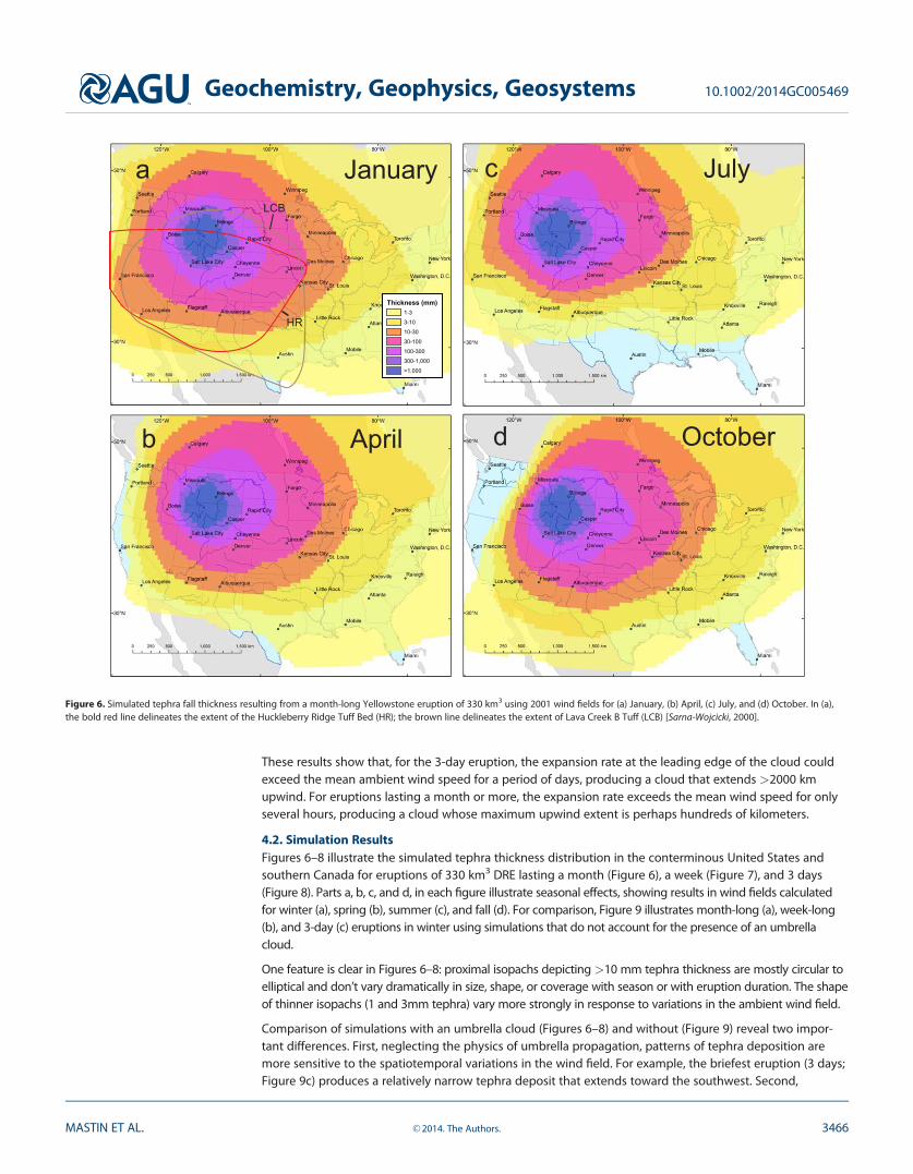
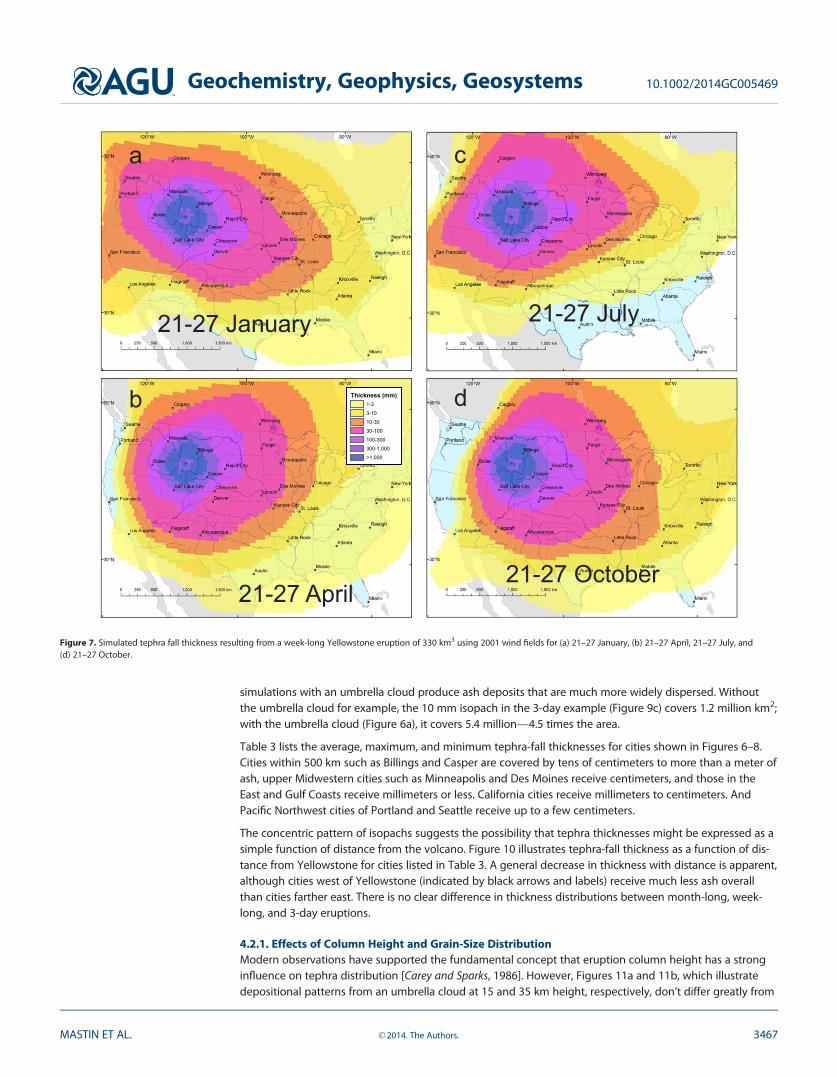
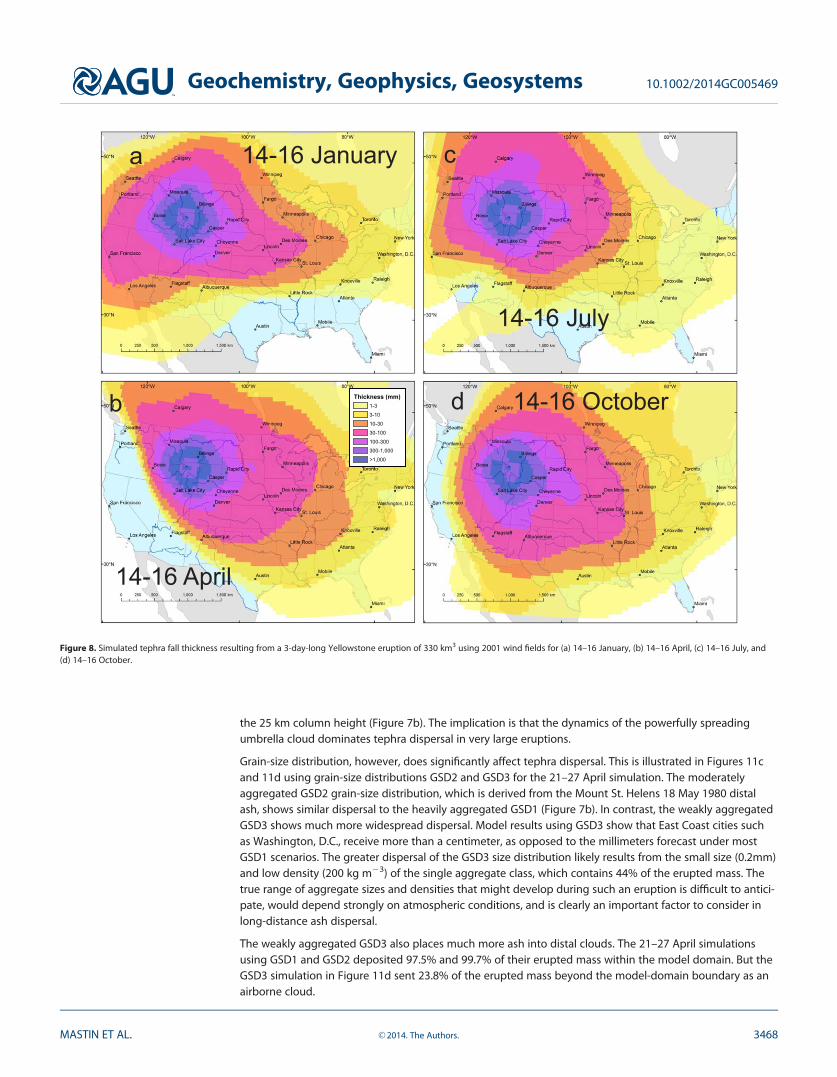
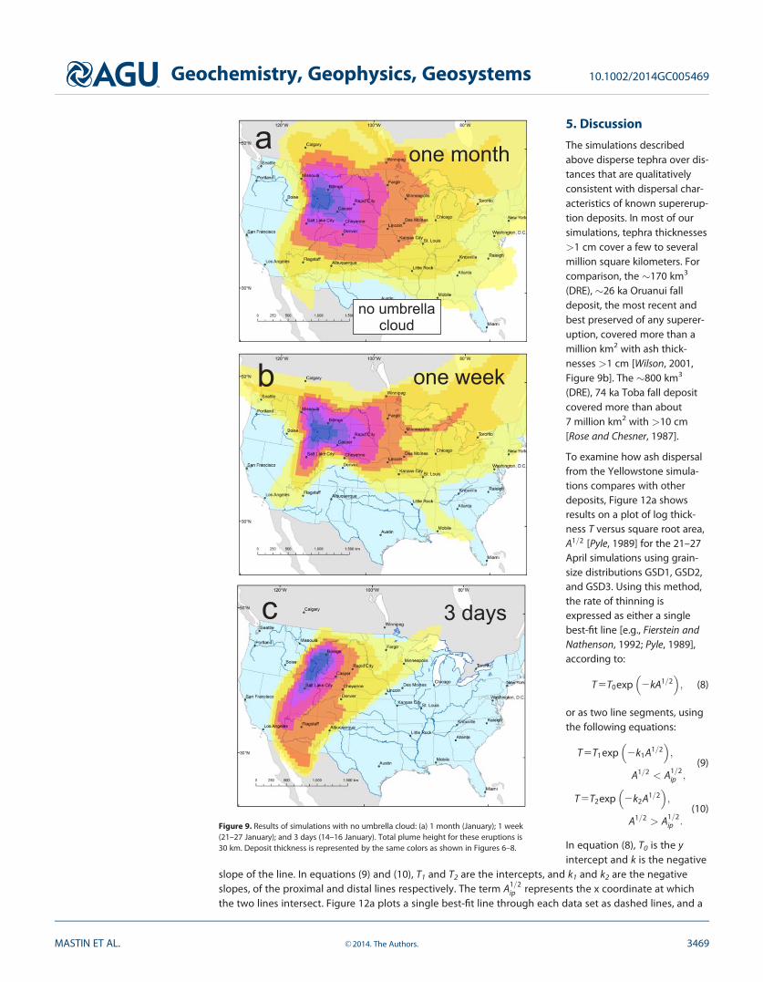
4.2. Simulation ResultsFigures 6–8 illustrate the simulated tephra thickness distribution in the conterminous United States andsouthern Canada for eruptions of 330 km3 DRE lasting a month (Figure 6), a week (Figure 7), and 3 days(Figure 8). Parts a, b, c, and d, in each figure illustrate seasonal effects, showing results in wind fields calculatedfor winter (a), spring (b), summer (c), and fall (d). For comparison, Figure 9 illustrates month-long (a), week-long(b), and 3-day (c) eruptions in winter using simulations that do not account for the presence of an umbrellacloud.

One feature is clear in Figures 6–8: proximal isopachs depicting >10 mm tephra thickness are mostly circular toelliptical and don’t vary dramatically in size, shape, or coverage with season or with eruption duration. The shapeof thinner isopachs (1 and 3mm tephra) vary more strongly in response to variations in the ambient wind field.

Comparison of simulations with an umbrella cloud (Figures 6–8) and without (Figure 9) reveal two impor-tant differences. First, neglecting the physics of umbrella propagation, patterns of tephra deposition aremore sensitive to the spatiotemporal variations in the wind field. For example, the briefest eruption (3 days;Figure 9c) produces a relatively narrow tephra deposit that extends toward the southwest. Second,

April

January

b

a

HR

LCB

Miami

Thickness (mm)1-3

3-10

10-30

30-100

100-300

300-1,000

>1,000

Octoberd

Julyc

Figure 6. Simulated tephra fall thickness resulting from a month-long Yellowstone eruption of 330 km3 using 2001 wind fields for (a) January, (b) April, (c) July, and (d) October. In (a),the bold red line delineates the extent of the Huckleberry Ridge Tuff Bed (HR); the brown line delineates the extent of Lava Creek B Tuff (LCB) [Sarna-Wojcicki, 2000].

Geochemistry, Geophysics, Geosystems 10.1002/2014GC005469

MASTIN ET AL. VC 2014. The Authors. 3466

simulations with an umbrella cloud produce ash deposits that are much more widely dispersed. Withoutthe umbrella cloud for example, the 10 mm isopach in the 3-day example (Figure 9c) covers 1.2 million km2;with the umbrella cloud (Figure 6a), it covers 5.4 million—4.5 times the area.

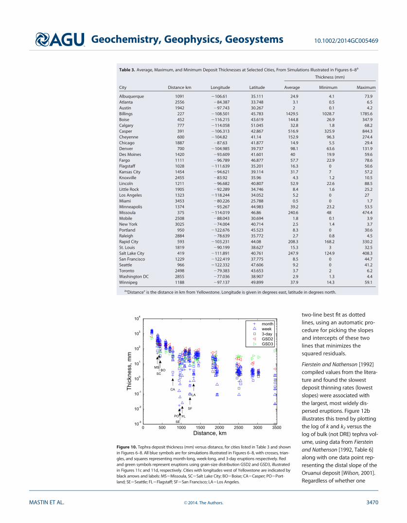
Table 3 lists the average, maximum, and minimum tephra-fall thicknesses for cities shown in Figures 6–8.Cities within 500 km such as Billings and Casper are covered by tens of centimeters to more than a meter ofash, upper Midwestern cities such as Minneapolis and Des Moines receive centimeters, and those in theEast and Gulf Coasts receive millimeters or less. California cities receive millimeters to centimeters. AndPacific Northwest cities of Portland and Seattle receive up to a few centimeters.

The concentric pattern of isopachs suggests the possibility that tephra thicknesses might be expressed as asimple function of distance from the volcano. Figure 10 illustrates tephra-fall thickness as a function of dis-tance from Yellowstone for cities listed in Table 3. A general decrease in thickness with distance is apparent,although cities west of Yellowstone (indicated by black arrows and labels) receive much less ash overallthan cities farther east. There is no clear difference in thickness distributions between month-long, week-long, and 3-day eruptions.

4.2.1. Effects of Column Height and Grain-Size DistributionModern observations have supported the fundamental concept that eruption column height has a stronginfluence on tephra distribution [Carey and Sparks, 1986]. However, Figures 11a and 11b, which illustratedepositional patterns from an umbrella cloud at 15 and 35 km height, respectively, don’t differ greatly from

21-27 January

a

21-27 April

b

Miami

Thickness (mm)1-3

3-10

10-30

30-100

100-300

300-1,000

>1,000

21-27 October

d

21-27 July

c

Figure 7. Simulated tephra fall thickness resulting from a week-long Yellowstone eruption of 330 km3 using 2001 wind fields for (a) 21–27 January, (b) 21–27 April, 21–27 July, and(d) 21–27 October.

Geochemistry, Geophysics, Geosystems 10.1002/2014GC005469

MASTIN ET AL. VC 2014. The Authors. 3467

the 25 km column height (Figure 7b). The implication is that the dynamics of the powerfully spreadingumbrella cloud dominates tephra dispersal in very large eruptions.

Grain-size distribution, however, does significantly affect tephra dispersal. This is illustrated in Figures 11cand 11d using grain-size distributions GSD2 and GSD3 for the 21–27 April simulation. The moderatelyaggregated GSD2 grain-size distribution, which is derived from the Mount St. Helens 18 May 1980 distalash, shows similar dispersal to the heavily aggregated GSD1 (Figure 7b). In contrast, the weakly aggregatedGSD3 shows much more widespread dispersal. Model results using GSD3 show that East Coast cities suchas Washington, D.C., receive more than a centimeter, as opposed to the millimeters forecast under mostGSD1 scenarios. The greater dispersal of the GSD3 size distribution likely results from the small size (0.2mm)and low density (200 kg m23) of the single aggregate class, which contains 44% of the erupted mass. Thetrue range of aggregate sizes and densities that might develop during such an eruption is difficult to antici-pate, would depend strongly on atmospheric conditions, and is clearly an important factor to consider inlong-distance ash dispersal.

The weakly aggregated GSD3 also places much more ash into distal clouds. The 21–27 April simulationsusing GSD1 and GSD2 deposited 97.5% and 99.7% of their erupted mass within the model domain. But theGSD3 simulation in Figure 11d sent 23.8% of the erupted mass beyond the model-domain boundary as anairborne cloud.

14-16 Januarya

14-16 April

b

Miami

Thickness (mm)1-3

3-10

10-30

30-100

100-300

300-1,000

>1,000

14-16 July

c

14-16 Octoberd

Figure 8. Simulated tephra fall thickness resulting from a 3-day-long Yellowstone eruption of 330 km3 using 2001 wind fields for (a) 14–16 January, (b) 14–16 April, (c) 14–16 July, and(d) 14–16 October.

Geochemistry, Geophysics, Geosystems 10.1002/2014GC005469

MASTIN ET AL. VC 2014. The Authors. 3468

5. Discussion

The simulations describedabove disperse tephra over dis-tances that are qualitativelyconsistent with dispersal char-acteristics of known supererup-tion deposits. In most of oursimulations, tephra thicknesses>1 cm cover a few to severalmillion square kilometers. Forcomparison, the �170 km3

(DRE), �26 ka Oruanui falldeposit, the most recent andbest preserved of any superer-uption, covered more than amillion km2 with ash thick-nesses >1 cm [Wilson, 2001,Figure 9b]. The �800 km3

(DRE), 74 ka Toba fall depositcovered more than about7 million km2 with >10 cm[Rose and Chesner, 1987].

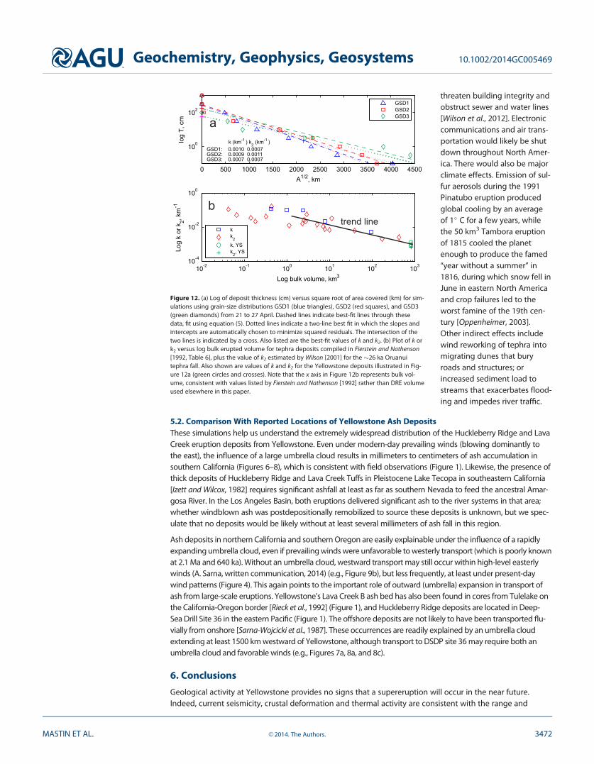
To examine how ash dispersalfrom the Yellowstone simula-tions compares with otherdeposits, Figure 12a showsresults on a plot of log thick-ness T versus square root area,A1=2 [Pyle, 1989] for the 21–27April simulations using grain-size distributions GSD1, GSD2,and GSD3. Using this method,the rate of thinning isexpressed as either a singlebest-fit line [e.g., Fierstein andNathenson, 1992; Pyle, 1989],according to:

T5T0exp 2kA1=2� �

; (8)

or as two line segments, usingthe following equations:

T5T1exp 2k1A1=2� �

;

A1=2 < A1=2ip ;

(9)

T5T2exp 2k2A1=2� �

;

A1=2 > A1=2ip :

(10)

In equation (8), T0 is the yintercept and k is the negative

slope of the line. In equations (9) and (10), T1 and T2 are the intercepts, and k1 and k2 are the negativeslopes, of the proximal and distal lines respectively. The term A1=2

ip represents the x coordinate at whichthe two lines intersect. Figure 12a plots a single best-fit line through each data set as dashed lines, and a

one month

no umbrellacloud

3 days

one week

a

b

c

Figure 9. Results of simulations with no umbrella cloud: (a) 1 month (January); 1 week(21–27 January); and 3 days (14–16 January). Total plume height for these eruptions is30 km. Deposit thickness is represented by the same colors as shown in Figures 6–8.

Geochemistry, Geophysics, Geosystems 10.1002/2014GC005469

MASTIN ET AL. VC 2014. The Authors. 3469

two-line best fit as dottedlines, using an automatic pro-cedure for picking the slopesand intercepts of these twolines that minimizes thesquared residuals.

Fierstein and Nathenson [1992]compiled values from the litera-ture and found the slowestdeposit thinning rates (lowestslopes) were associated withthe largest, most widely dis-persed eruptions. Figure 12billustrates this trend by plottingthe log of k and k2 versus thelog of bulk (not DRE) tephra vol-ume, using data from Fiersteinand Nathenson [1992, Table 6]along with one data point rep-resenting the distal slope of theOruanui deposit [Wilson, 2001].Regardless of whether one

Table 3. Average, Maximum, and Minimum Deposit Thicknesses at Selected Cities, From Simulations Illustrated in Figures 6–8a

City Distance km Longitude Latitude

Thickness (mm)

Average Minimum Maximum

Albuquerque 1091 2106.61 35.111 24.9 4.1 73.9Atlanta 2556 284.387 33.748 3.1 0.5 6.5Austin 1942 297.743 30.267 2 0.1 4.2Billings 227 2108.501 45.783 1429.5 1028.7 1785.6Boise 452 2116.215 43.619 144.8 26.9 347.9Calgary 777 2114.058 51.045 32.8 1.8 68.2Casper 391 2106.313 42.867 516.9 325.9 844.3Cheyenne 600 2104.82 41.14 152.9 96.3 274.4Chicago 1887 287.63 41.877 14.9 5.5 29.4Denver 700 2104.985 39.737 98.1 63.6 131.9Des Moines 1420 293.609 41.601 40 19.9 59.6Fargo 1111 296.789 46.877 57.7 22.9 78.6Flagstaff 1028 2111.639 35.201 16.3 0 50.6Kansas City 1454 294.621 39.114 31.7 7 57.2Knoxville 2455 283.92 35.96 4.3 1.2 10.5Lincoln 1211 296.682 40.807 52.9 22.6 88.5Little Rock 1905 292.289 34.746 8.4 1.6 25.2Los Angeles 1323 2118.244 34.052 5.2 0 27Miami 3453 280.226 25.788 0.5 0 1.7Minneapolis 1374 293.267 44.983 39.2 23.2 53.5Missoula 375 2114.019 46.86 240.6 48 474.4Mobile 2508 288.043 30.694 1.8 0.1 3.9New York 3025 274.004 40.714 2.5 1.4 3.7Portland 950 2122.676 45.523 8.3 0 30.6Raleigh 2884 278.639 35.772 2.7 0.8 4.5Rapid City 593 2103.231 44.08 208.3 168.2 330.2St. Louis 1819 290.199 38.627 15.3 3 32.5Salt Lake City 419 2111.891 40.761 247.9 124.9 408.3San Francisco 1229 2122.419 37.775 8.5 0 44.7Seattle 966 2122.332 47.606 9.2 0 41.2Toronto 2498 279.383 43.653 3.7 2 6.2Washington DC 2855 277.036 38.907 2.9 1.3 4.4Winnipeg 1188 297.137 49.899 37.9 14.3 59.1

a‘‘Distance’’ is the distance in km from Yellowstone. Longitude is given in degrees east, latitude in degrees north.

0 500 1000 1500 2000 2500 3000 350010-3

10-2

10-1

100

101

102

103

104

BO

CA

FL

LA

MS

PO

SC

SF

SE

Distance, km

Thic

knes

s, m

m

monthweek3-dayGSD2GSD3

Figure 10. Tephra deposit thickness (mm) versus distance, for cities listed in Table 3 and shownin Figures 6–8. All blue symbols are for simulations illustrated in Figures 6–8, with crosses, trian-gles, and squares representing month-long, week-long, and 3-day eruptions respectively. Redand green symbols represent eruptions using grain-size distribution GSD2 and GSD3, illustratedin Figures 11c and 11d, respectively. Cities with longitudes west of Yellowstone are indicated byblack arrows and labels: MS5Missoula, SC5Salt Lake City; BO5Boise; CA5Casper; PO5Port-land; SE5Seattle; FL5Flagstaff; SF5San Francisco; LA5Los Angeles.

Geochemistry, Geophysics, Geosystems 10.1002/2014GC005469

MASTIN ET AL. VC 2014. The Authors. 3470

considers the total data set or separates out points for k or k2, a downward trend with increasing volume isvisible at volumes >�1 km3. At the right side of the plot, lying along the trend line, are values of k and k2

from the three Yellowstone simulations in Figure 12a. Their location along this trend line suggests that thesimulated tephra dispersal is reasonable for an eruption of this size.

These results portray a dramatically different picture of the ashfall hazard from a caldera-forming supererup-tion than one might expect based on traditional tephra transport models, which tend to neglect the physicsof an expanding umbrella cloud. The distribution of tephra from such a large eruption is less sensitive to thewind field than that of smaller eruptions. It is also more widespread, and radially symmetric about the vent.The wide dispersal of tephra in our simulations results from rapid expansion of the umbrella rather from thana high plume or variability in the wind field at the umbrella spreading level during prolonged activity.

5.1. Immediate Ash Thickness Versus Long-Term ImpactNorth America’s highest population density lies along its coastlines. Deposit thicknesses on the coasts fromnearly all simulations is millimeters to a few centimeters. Thicknesses of this magnitude seem small but theireffects are far from negligible. A few millimeters of ash can reduce traction on roads and runways [Guffantiet al., 2009], short out electrical transformers [Wilson et al., 2012] and cause respiratory problems [Horwelland Baxter, 2006]. Ash fall thicknesses of centimeters throughout the American Midwest would disrupt live-stock and crop production, especially during critical times in the growing season. Thick deposits could

April 21-2715 kma

April 21-2735 kmb

Miami

Thickness (mm)1-3

3-10

10-30

30-100

100-300

300-1,000

>1,000

April 21-27GSD2

c

April 21-27GSD3d

Miami

Thickness (mm)1-3

3-10

10-30

30-100

100-300

300-1,000

>1,000

Figure 11. Tephra fall thickness for simulations from 21 to 27 April, using (a) a 15 km umbrella-cloud height, (b) a 35 km umbrella-cloud height, (c) grain-size distribution GSD2, and(d) grain-size distribution GSD3.

Geochemistry, Geophysics, Geosystems 10.1002/2014GC005469

MASTIN ET AL. VC 2014. The Authors. 3471

threaten building integrity andobstruct sewer and water lines[Wilson et al., 2012]. Electroniccommunications and air trans-portation would likely be shutdown throughout North Amer-ica. There would also be majorclimate effects. Emission of sul-fur aerosols during the 1991Pinatubo eruption producedglobal cooling by an averageof 1� C for a few years, whilethe 50 km3 Tambora eruptionof 1815 cooled the planetenough to produce the famed‘‘year without a summer’’ in1816, during which snow fell inJune in eastern North Americaand crop failures led to theworst famine of the 19th cen-tury [Oppenheimer, 2003].Other indirect effects includewind reworking of tephra intomigrating dunes that buryroads and structures; orincreased sediment load tostreams that exacerbates flood-ing and impedes river traffic.

5.2. Comparison With Reported Locations of Yellowstone Ash DepositsThese simulations help us understand the extremely widespread distribution of the Huckleberry Ridge and LavaCreek eruption deposits from Yellowstone. Even under modern-day prevailing winds (blowing dominantly tothe east), the influence of a large umbrella cloud results in millimeters to centimeters of ash accumulation insouthern California (Figures 6–8), which is consistent with field observations (Figure 1). Likewise, the presence ofthick deposits of Huckleberry Ridge and Lava Creek Tuffs in Pleistocene Lake Tecopa in southeastern California[Izett and Wilcox, 1982] requires significant ashfall at least as far as southern Nevada to feed the ancestral Amar-gosa River. In the Los Angeles Basin, both eruptions delivered significant ash to the river systems in that area;whether windblown ash was postdepositionally remobilized to source these deposits is unknown, but we spec-ulate that no deposits would be likely without at least several millimeters of ash fall in this region.

Ash deposits in northern California and southern Oregon are easily explainable under the influence of a rapidlyexpanding umbrella cloud, even if prevailing winds were unfavorable to westerly transport (which is poorly knownat 2.1 Ma and 640 ka). Without an umbrella cloud, westward transport may still occur within high-level easterlywinds (A. Sarna, written communication, 2014) (e.g., Figure 9b), but less frequently, at least under present-daywind patterns (Figure 4). This again points to the important role of outward (umbrella) expansion in transport ofash from large-scale eruptions. Yellowstone’s Lava Creek B ash bed has also been found in cores from Tulelake onthe California-Oregon border [Rieck et al., 1992] (Figure 1), and Huckleberry Ridge deposits are located in Deep-Sea Drill Site 36 in the eastern Pacific (Figure 1). The offshore deposits are not likely to have been transported flu-vially from onshore [Sarna-Wojcicki et al., 1987]. These occurrences are readily explained by an umbrella cloudextending at least 1500 km westward of Yellowstone, although transport to DSDP site 36 may require both anumbrella cloud and favorable winds (e.g., Figures 7a, 8a, and 8c).

6. Conclusions

Geological activity at Yellowstone provides no signs that a supereruption will occur in the near future.Indeed, current seismicity, crustal deformation and thermal activity are consistent with the range and

0 500 1000 1500 2000 2500 3000 3500 4000 4500

100

102

A1/2, kmlo

g T,

cm

k (km-1 ) k2 (km-1 ) GSD1: 0.0010 0.0007GSD2: 0.0009 0.0011GSD3: 0.0007 0.0007

GSD1GSD2GSD3

10-2 10-1 100 101 102 10310-4

10-2

100

Log bulk volume, km3

Log

k or

k2, k

m-1

kk

2k, YSk2, YS

a

btrend line

Figure 12. (a) Log of deposit thickness (cm) versus square root of area covered (km) for sim-ulations using grain-size distributions GSD1 (blue triangles), GSD2 (red squares), and GSD3(green diamonds) from 21 to 27 April. Dashed lines indicate best-fit lines through thesedata, fit using equation (5). Dotted lines indicate a two-line best fit in which the slopes andintercepts are automatically chosen to minimize squared residuals. The intersection of thetwo lines is indicated by a cross. Also listed are the best-fit values of k and k2. (b) Plot of k ork2 versus log bulk erupted volume for tephra deposits compiled in Fierstein and Nathenson[1992, Table 6], plus the value of k2 estimated by Wilson [2001] for the �26 ka Oruanuitephra fall. Also shown are values of k and k2 for the Yellowstone deposits illustrated in Fig-ure 12a (green circles and crosses). Note that the x axis in Figure 12b represents bulk vol-ume, consistent with values listed by Fierstein and Nathenson [1992] rather than DRE volumeused elsewhere in this paper.

Geochemistry, Geophysics, Geosystems 10.1002/2014GC005469

MASTIN ET AL. VC 2014. The Authors. 3472

magnitude of signals observed his-torically over the past century[Lowenstern et al., 2006]. Over thepast two million years, trends inthe volume of eruptions and themagnitude of crustal melting maysignal a decline of major volca-nism from the Yellowstone region[Christiansen et al., 2007; Wattset al., 2012]. These factors, plus the3-in-2.1-million annual frequencyof past events, suggest a confi-dence of at least 99.9% that 21st-century society will not experience

a Yellowstone supereruption. But over the span of geologic time, supereruptions have recurred somewhereon Earth every 100,000 years on average [Mason et al., 2004; Sparks et al., 2005]. As such, it is important tocharacterize the potential effects of such events. We hope this work stimulates further examination of ashtransport during very large eruptions.

Appendix A: Simulating the Growth of the Pinatubo Umbrella Cloud

We validate the umbrella cloud formulation by simulating the growth of the 15 June 1991 umbrella cloud at Pina-tubo. This is the only large umbrella cloud observed with modern techniques and its growth has been examined innumerous studies. The model setup and atmospheric parameters are indicated in Table A1. For meteorological con-ditions we use the RE1 wind field. Typhoon Yunya prevented the launching of radiosondes during the eruption[Fero et al., 2009] and limited the accuracy of modeled wind fields. Thus we, like others [Costa et al., 2013; Fero et al.,2009], had to rotate wind directions 30 degrees counterclockwise to match the observed direction of cloudmovement.

Our umbrella-cloud formulation requires a single eruptive pulse of constant rate and umbrella-cloudheight. We use a starting time at 1340 Pinatubo Daylight Time (0440 UTC) on 15 June 1991; a duration of9 h; and an umbrella-cloud height of 25 km, which corresponds to the cloud top observed in satelliteimages [Holasek et al., 1996; Koyaguchi and Tokuno, 1993], but is lower than the 35–40 km of theovershooting top [Holasek et al., 1996]. The erupted volume has been estimated 4.8–6.0 km3 DRE fromdeposits [Wiesner et al., 2004, 2005]. We use an erupted volume of 6 km3 DRE, and assume a magma densityof 2500 kg m23.

Figure A1 (a) shows hourly outlines of the observed cloud perimeter starting at 1440 PDT, digitized fromFig. 5b of Holasek et al. [1996]. Figure A1 (b) shows outlines of the cloud at the same times, based on theAsh3d simulation. The result illustrates reasonably good agreement. Figure A2 shows cloud diameter versustime obtained from the observations of Holasek et al. [1996, Fig. 5b], from the Ash3d simulation, and fromsame theoretical method used in Fig. 5a, assuming an erupted volume of 6 (dashed line) or 10 (solid line)km3 DRE. For the Holasek et al. and Ash3d results, cloud diameter d was determined by measuring the cloudarea A and using the formula d 5 2sqrt(A/p). The Ash3d cloud diameters agree surprisingly well with thoseof Holasek et al., especially given that the simulation assumed a constant eruption rate with time.

ReferencesBacon, C. R. (1983), Eruptive history of Mount Mazama and Crater Lake Caldera, Cascade Range, U.S.A., J. Volcanol. Geotherm. Res., 18, 57–115.Baines, P. G., and R. S. J. Sparks (2005), Dynamics of giant volcanic ash clouds from supervolcanic eruptions, Geophys. Res. Lett., 32, L24808,

doi:10.1029/2005GL024597.Bonadonna, C., J. C. Phillips, and B. F. Houghton (2005), Modeling tephra sedimentation from a Ruapehu weak plume eruption, J. Geophys.

Res., 110, B08209, doi:10.1029/2004JB003515.Carey, S., and R. S. J. Sparks (1986), Quantitative models of the fallout and dispersal of tephra from volcanic eruption columns, Bull. Volca-

nol., 48, 109–125.Christiansen, R. L. (2001), The Quaternary and Pliocene Yellowstone Plateau Volcanic Field of Wyoming, Idaho, and Montana, U.S. Geol.

Surv. Prof. Pap. 729-G, U.S. Gov. Print. Off., Washington, D. C.Christiansen, R. L., and H. R. Blank Jr. (1972), Volcanic stratigraphy of the Quaternary rhyolite plateau in Yellowstone National Park, Wyom-

ing, U.S. Geol. Surv. Prof. Pap., 729-B, 18 pp.

Table A1. Model Parameters Used to Simulate Growth of the 15 June 1991 UmbrellaCloud at Pinatubo

Parameter Value(s)

Eruption start time (UTC) 15 Jun 1991, 0440UTC (1340 local time)Height of top of umbrella cloud 25 kmDuration 9 hErupted volume 6 km3 DRE (1.531013 kg)Model domain 89.558–132.454� longitude 1.227–28.846� latitudeModel resolution 0.2� horizontally, 2 km verticallyGrain sizes One grain size 0.01 mm diameter 1000 kg m23 densityDiffusion constant 0 m2 s21

ke 0.1N 0.02 s21

C 0.53104 m3 kg23/4s27/8

k 0.2

AcknowledgmentsWe thank reviewers Andrei Sarna-Wojcicki, Robert L. Christiansen, andManuel Nathenson for comments thatimproved the paper. We would alsolike to express our gratitude to ananonymous reviewer whorecommended incorporation of anexpanding umbrella cloud into Ash3d,and pointed us to the approach ofCosta et al. [2013]. Second author AVEacknowledges NSF PostdoctoralFellowship EAR1250029 for funding atthe time of her contribution to thiswork. The data and model results usedin this paper have been posted assupporting information. Thesupporting information includes inputfiles and ASCII or kmz output files thatcan be opened in ArcMapVR or GoogleEarthVR software (use of trade namesdoes not imply endorsement of theseproducts by the U.S. Government).

Geochemistry, Geophysics, Geosystems 10.1002/2014GC005469

MASTIN ET AL. VC 2014. The Authors. 3473

Christiansen, R. L., J. B. Lowenstern, R. B. Smith, H. Heasler, L. A. Morgan, M. Nathenson, L. G. Mastin, L. J. P. Muffler, and J. E. Robinson(2007), Preliminary assessment of volcanic and hydrothermal hazards in Yellowstone National Park and vicinity, U.S. Geol. Surv. OpenFile Rep. 2007-1071, p. 94, U.S. Gov. Print. Off., Washington, D. C.

Cornell, W., S. Carey, and H. Sigurdsson (1983), Computer simulation of transport and deposition of the campanian Y-5 ash, J. Volcanol. Geo-therm. Res., 17(1-4), 89–109.

Costa, A., A. Folch, and G. Macedonio (2013), Density-driven transport in the umbrella region of volcanic clouds: Implications for tephra dis-persion models, Geophys. Res. Lett., 40, 4823–4827, doi:10.1002/grl.50942.

Cramp, A., C. Vitaliano, and M. Collins (1989), Identification and dispersion of the campanian ash layer (Y-5) in the sediments of the EasternMediterranean, Geo Mar. Lett., 9(1), 19–25, doi:10.1007/BF02262814.

Di Lorenzo, E., K. M. Cobb, J. C. Furtado, N. Schneider, B. T. Anderson, A. Bracco, M. A. Alexander, and D. J. Vimont (2010), Central Pacific ElNino and decadal climate change in the North Pacific Ocean, Nat. Geosci., 3(11), 762–765. [Available at http://www.nature.com/ngeo/journal/v3/n11/abs/ngeo984.html#supplementary-information.]

Dobson, P. F., L. Sienkiewicz, and R. A. Armin (1991), Origin of thick ash-rich sediments in the northern Gulf of Mexico, Geol. Soc. Am. Abstr.Programs, 23(5), A258.

Durant, A. J., W. I. Rose, A. M. Sarna-Wojcicki, S. Carey, and A. C. Volentik (2009), Hydrometeor-enhanced tephra sedimentation: Constraintsfrom the 18 May 1980 eruption of Mount St. Helens (USA), J. Geophys. Res., 114, B03204, doi:10.1029/2008JB005756.

Fero, J., S. N. Carey, and J. T. Merrill (2009), Simulating the dispersal of tephra from the 1991 Pinatubo eruption: Implications for the forma-tion of widespread ash layers, J. Volcanol. Geotherm. Res., 186(1–2), 120–131, doi:10.1016/j.jvolgeores.2009.03.011.

Fierstein, J., and M. Nathenson (1992), Another look at the calculation of fallout tephra volumes, Bull. Volcanol., 54, 156–167.Folch, A., A. Costa, and G. Macedonio (2009), FALL3D: A computational model for transport and deposition of volcanic ash, Comput. Geosci.,

35(6), 1334–1342, doi:10.1016/j.cageo.2008.08.008.Gudmundsson, M. T., et al. (2012), Ash generation and distribution from the April-May 2010 eruption of Eyjafjallaj€okull, Iceland, Sci. Rep.,

2(572), doi:10.1038/srep00572.Guffanti, M., G. Mayberry, T. Casadevall, and R. Wunderman (2009), Volcanic hazards to airports, Nat. Hazards, 51(2), 287–302, doi:10.1007/

s11069-008-9254-2.Hildreth, W. (1983), The compositionally zoned eruption of 1912 in the Valley of Ten Thousand Smokes, Katmai National Park, Alaska, J. Vol-

canol. Geotherm. Res., 18, 1–56.Hildreth, W. and R. E. Drake (1992), Volc�an Quizapu, Chilean Andes, Bull. Volcanol., 54, 93–125.Holasek, R. E., S. Self and A. W. Woods (1996), Satellite observations and interpretation of the 1991 Mount Pinatubo eruption plumes,

J. Geophys. Res., 101(B12), 27,635–27,656, doi:10.1029/96JB01179.Horwell, C. J., and P. J. Baxter (2006), The respiratory health hazards of volcanic ash: A review for volcanic risk mitigation, Bull. Volcanol.,

69(1), 1–24, doi:10.1007/s00445-006-0052-y.Izett, G. A., and R. E. Wilcox (1982), Map showing locallities and inferred distributions of the Huckleberry Ridge, Mesa Falls and Lava Creek

ash beds (Pearlette family ash beds) of Pliocene and Pleistocene age in the western United States and southern Canada, U.S. Geol. Surv.Misc. Invest. Map I-1325, scale 1:4,000,000, U.S. Geological Survey, Washington, D. C.

Kalnay, E., et al. (1996), The NCEP/NCAR 40-Year Reanalysis Project, Bull. Am. Meteorol. Soc., 77(3), 437–471, doi:10.1175/1520-0477(1996)077<0437:TNYRP>2.0.CO;2.

Koyaguchi, T., and M. Ohno (2001), Reconstruction of eruption column dynamics on the basis of grain size of tephra fall deposits: 2. Appli-cation to the Pinatubo 1991 eruption, J. Geophys. Res., 106(B4), 6513–6533, doi:10.1029/2000JB900427.

Koyaguchi, T., and M. Tokuno (1993), Origin of the giant eruption cloud of Pinatubo, June 15, 1991, J. Volcanol. Geotherm. Res., 55, 85–96.Lowenstern, J. B., R. B. Smith, and D. P. Hill (2006), Monitoring super-volcanoes: Geophysical and geochemical signals at Yellowstone and

other large caldera systems, Philos. Trans. R. Soc. A, 364(1845), 2055–2072, doi:10.1098/rsta.2006.1813.Mantua, N. J., and S. R. Hare (2002), The Pacific decadal oscillation, J. Oceanogr., 58(1), 35–44, doi:10.1023/A:1015820616384.Mason, B. G., D. M. Pyle, and C. Oppenheimer (2004), The size and frequency of the largest eruptions on Earth, Bulletin of Volcanology,

vol. 66, pp. 735–748, doi:10.1007/s00445-004-0355-9.Mastin, L. G., et al. (2009), A multidisciplinary effort to assign realistic source parameters to models of volcanic ash-cloud transport and dis-

persion during eruptions, J. Volcanol. Geotherm. Res., 186, 10–21.Mastin, L. G., A. Van Eaton, A. Durant, H. Schwaiger, and R. Denlinger (2013a), Towards an operational implementation of particle aggrega-

tion in ash dispersion models, Abstract V21D-04 presented at 2013 Fall Meeting, AGU, San Francisco, Calif.Mastin, L. G., H. Schwaiger, D. J. Schneider, K. L. Wallace, J. Schaefer, and R. P. Denlinger (2013b), Injection, transport, and deposition of

tephra during event 5 at Redoubt Volcano, 23 March, 2009, J. Volcanol. Geotherm. Res., 259, 201–213, doi:10.1016/j.jvolgeores.2012.04.025.

Morton, B. R., G. I. Taylor, and J. S. Turner (1956), Turbulent gravitational convection from maintained and instantaneous sources, Proc. R.Soc. London, Ser. A, 234, 1–23.

Newhall, C. G., and R. Punongbayan (Eds.) (1996), Fire and Mud: Eruptions and Lahars of Mount Pinatubo, Philippines, 1126 pp., Univ. ofWash. Press, Seattle.

Oppenheimer, C. (2003), Climatic, environmental and human consequences of the largest known historic eruption: Tambora volcano(Indonesia) 1815, Prog. Phys. Geogr., 27(2), 230–259, doi:10.1191/0309133303pp379ra.

Pallister, J. S., R. P. Hoblitt, D. R. Crandell, and D. R. Mullineaux (1992), Mount St. Helens a decade after the 1980 eruptions: Magmatic mod-els, chemical cycles, and a revised hazards assessment, Bull. Volcanol., 54, 126–146.

Pyle, D. M. (1989), The thickness, volume and grain size of tephra fall deposits, Bull. Volcanol., 51, 1–15.Rieck, H. J., A. M. Sarna-Wojcicki, C. E. Meyer, and D. P. Adam (1992), Magnetostratigraphy and tephrochronology of an upper Pliocene to

Holocene record in lake sediments at Tulelake, northern California, Geol. Soc. Am. Bull., 104(4), 409–428, doi:10.1130/0016–7606(1992)104<0409:matoau>2.3.co;2.

Rose, W. I., and C. A. Chesner (1987), Dispersal of ash in the great Toba eruption, 75 ka, Geology, 15(10), 913–917, doi:10.1130/0091–7613(1987)15<913:doaitg>2.0.co;2.

Sarna-Wojcicki, A. M. (2000), Tephrochronology, in Quaternary Geochronology: Methods and Applications, AGU Ref. Shelf 4, edited by J. S.Noller, J. M. Sowers, and W. R. Lettis, pp. 357–377, AGU, Washington, D. C.

Sarna-Wojcicki, A. M., S. D. Morrison, C. E. Meyer, and J. W. Hillhouse (1987), Correlation of upper Cenozoic tephra layers between sedi-ments of the western United States and eastern Pacific Ocean and comparison with biostratigraphic and magnetostratigraphic agedata, Geol. Soc. Am. Bull., 98(2), 207–223, doi:10.1130/0016-7606(1987)98<207:couctl>2.0.co;2.

Geochemistry, Geophysics, Geosystems 10.1002/2014GC005469

MASTIN ET AL. VC 2014. The Authors. 3474

Schwaiger, H., R. Denlinger, and L. G. Mastin (2012), Ash3d: A finite-volume, conservative numerical model for ash transport and tephradeposition, J. Geophys. Res., 117, B04204, doi:10.1029/2011JB008968.

Self, S. (2006), The effects and consequences of very large explosive volcanic eruptions, Philos. Trans. R. Soc. A, 364, 2073–2097, doi:10.1098/rsta.2006.1814.

Self, S., M. R. Rampino, M. S. Newton, and J. Wolff (1984), Volcanological study of the great Tambora eruption of 1815, Geology, 12(11),659–663.

Simkin, T. L., and R. S. Fiske (1983), Krakatau 1883: The Volcanic Eruption and Its Effects, 464 pp., Smithsonian Inst., Washington, D. C.Sorem, R. K. (1982), Volcanic ash clusters: Tephra rafts and scavengers, J. Volcanol. Geotherm. Res., 13, 63–71.Sparks, R. S. J. (1986), The dimensions and dynamics of volcanic eruption columns, Bull. Volcanol., 48(1), 3–15, doi:10.1007/BF01073509.Sparks, R. S. J., J. G. Moore and C. J. Rice (1986), The initial giant umbrella cloud of the May 18th, 1980, explosive eruption of Mount St. Hel-

ens, J. Volcanol. Geotherm. Res., 28(3-4), 257–274.Sparks, R. S. J., M. I. Bursik, S. N. Carey, J. S. Gilbert, L. S. Glaze, H. Sigurdsson and A. W. Woods (1997), Volcanic Plumes, 574 pp., John Wiley,

Chichester, U. K.Sparks, R. S. J., S. Self, J. Gratten, C. Oppenheimer, D. M. Pyle, and H. Rymer (2005), Supereruptions: Global Effects and Future Threats, Report

of a Geological Society Working Group, 25 pp., Geological Society of London, London, U. K.Suzuki, T. (1983), A Theoretical model for dispersion of tephra, in Arc Volcanism: Physics and Tectonics, edited by D. Shimozuru and I.

Yokoyama, pp. 95–113, Terra Sci. Publ. Co., Tokyo.Suzuki, Y. J., and T. Koyaguchi (2009), A three-dimensional numerical simulation of spreading umbrella clouds, J. Geophys. Res., 114,

B03209, doi:10.1029/2007JB005369.Van Eaton, A. R., J. D. Muirhead, C. J. N. Wilson and C. Cimarelli (2012), Growth of volcanic ash aggregates in the presence of liquid water

and ice: An experimental approach, Bull. Volcanol., 74(9), 1963–1984, doi:10.1007/s00445-012-0634-9.Wallace, K. L., J. R. Schaefer, and M. L. Coombs (2013), Character, mass, distribution, and origin of tephra-fall deposits from the 2009 erup-

tion of Redoubt Volcano, Alaska—Highlighting the significance of particle aggregation, J. Volcanol. Geotherm. Res., 259, 145–169, doi:10.1016/j.jvolgeores.2012.09.015.

Watts, K. E., I. Bindeman, and A. K. Schmitt (2012), Crystal-scale anatomy of a dying supervolcano: An isotope and geochronology study ofindividual phenocrysts from voluminous rhyolites of the Yellowstone Caldera, Contrib. Mineral. Petrol., 164, 45–67.

Wiesner, M., A. Wetzel, S. Catane, E. Listanco, and H. Mirabueno (2004), Grain size, areal thickness distribution and controls on sedimenta-tion of the 1991 Mount Pinatubo tephra layer in the South China Sea, Bull. Volcanol., 66(3), 226–242, doi:10.1007/s00445-003-0306-x.

Wiesner, M., A. Wetzel, S. Catane, E. Listanco, and H. Mirabueno (2005), Grain size, areal thickness distribution and controls on sedimenta-tion of the 1991 Mount Pinatubo tephra layer in the South China Sea, Bull. Volcanol., 67(5), 490–495, doi:10.1007/s00445-005-0421-y.

Wilcox, R. E., and C. W. Naeser (1992), The Pearlette family ash beds in the Great Plains: Finding their identities and their roots in the Yel-lowstone country, Quat. Int., 13–14, 9–13, doi:10.1016/1040-6182(92)90003-K.

Wilson, C. J. N. (2001), The 26.5ka Oruanui eruption, New Zealand: An introduction and overview, J. Volcanol. Geotherm. Res., 112(1–4), 133–174, doi:10.1016/S0377-0273(01)00239-6.

Wilson, C. J. N. (2008), Supereruptions and supervolcanoes: Processes and products, Elements, 4, 29–34.Wilson, C. J. N., and W. Hildreth (1997), The Bishop Tuff: New insights from eruptive stratigraphy, J. Geol., 105, 407–439.Wilson, L., and T. C. Huang (1979), The influence of shape on the atmospheric settling velocity of volcanic ash particles, Earth Planet. Sci.

Lett., 44, 311–324.Wilson, T. M., C. Stewart, V. Sword-Daniels, G. S. Leonard, D. M. Johnston, J. W. Cole, J. Wardman, G. Wilson and S. T. Barnard (2012), Volcanic

ash impacts on critical infrastructure, Phys. Chem. Earth, 45–46, 5–23, doi:10.1016/j.pce.2011.06.006.

Geochemistry, Geophysics, Geosystems 10.1002/2014GC005469

MASTIN ET AL. VC 2014. The Authors. 3475