ELSEYIER Journal of Geometry and Physics 32 (2000) 293-3 10

IOURNAL OF

GEOMETRYAND

PHYSICS

Geodesics with prescribed energy on static Lorentzian manifolds with convex boundary *

Rossella Bartolo ayh,1, Anna Germinario ‘-* a Departamento de Geometria y Topologia, Fat. Ciencias, Univ. Granada,

Avenida Fuentenueva s/n. 18071 Granada, Spain b Dipartimento Interuniversitario di Matematica, Politecnico di Bari,

Via E. Orabona, 4, 70125 Bari, Italy c Dipartimento Interuniversitario di Matematica, Universitri degli Studi di Bari,

Via E. Orabona, 4, 70125 Bari, Italy

Received 12 January 1999; received in revised form 23 April 1999

Abstract

By using some variational principles and the Ljustemik-Schnirelmann critical point theory, we extend some previous results dealing with the existence and multiplicity of geodesics having prescribed energy joining a point with a line on static Lorentzian manifolds with convex boundary. Our techniques work also in the case of timelike and spacelike geodesics on manifolds with boundary and for a physically relevant class of spacetimes with non-smooth boundary. 0 2000 Elsevier Science B.V. All rights reserved.

Subj. Class.: Differential geometry; General relativity 1991 MSC: 58E05; 58ElO; 53C50 Keywords: Geodesics; Static Lorentzian manifolds

1. Introduction

In this paper we study the existence and multiplicity of geodesics having a prescribed pa- rameterization proportional to the arc length, joining a point with a line on a static Lorentzian

manifold with convex boundary. We recall that a Lorentzian manifold (M, (. , .) (~1) is a finite dimensional manifold M with a smooth, symmetric tensor field (. , .)(L, which is a

*Work supported by MURST (ex 40% and 60 % research funds). * Corresponding author. ’ Part of the Ph.D. thesis of this author is contained in this paper.

0393~0440/00/$ - see front matter 0 2000 Elsevier Science B.V. All rights reserved PII: s0393-0440(99)00034-0

294 R. Bartolo, A. Germinario/Journal of Geometry and Physics 32 (2000) 293-310

non-degenerate scalar product with index one on each T,M, for any z E M, (see e.g. [ 1 l] for more details). A geodesic is a curve y :]a, b[+ M satisfying

D,p = 0,

where D, denotes the covariant derivative induced by the Levi-Civita connection on M. It is easy to see that, if y :]a, b[-+ M is a geodesic, there exists a constant E = E(y) E R’ independent of s such that for any s ~]a, b[

E = &(3(s), P(S))(L).

In the sequel we shall call the constant E energy. We point out that such a name is not re- lated to its physical meaning. A geodesic y is said timelike (respectively lightlike, spacelike) if E is negative (respectively null, positive). Four-dimensional Lorentzian manifolds are the mathematical models of relativistic spacetimes. In General Relativity, lightlike geodesics represent light rays and timelike geodesics the world-lines of free falling particles.

Here we shall consider the class of static Lorentzian manifolds.

Definition 1.1. Let (MO, (., .)) be a connected Riemannian manifold and set M = MO x R. A (standard) static Lorentzian metric (. , .) CL,) on M is defined in the following way: for any z = (x, t) E M and for any 5‘ = (c, t), (“ = (c’, t’) E TzM = TxMo x Iw

(53 5’)(L) = (63 (7 - B(x>tr’, (1.1)

where B : MO + R is a smooth positive function. The couple (M, (. , a) CL)) is said static Lorentzian manifold.

Moreover we shall assume that M = MO x R is a static Lorentzian manifold with convex boundary.

Definition 1.2. Let M be an open subset of a manifold 5 with topological boundary i3M. We say that M has convex boundary if for any geodesic y : [a, b] + M U aM such that

v(a), y(b) E M

~(]a, bl) c M. (1.2)

If aM is smooth, using the distance from the boundary, it can be proved that there exists a smooth function # : 2 --+ R such that

M = {z E i+D(z) > O), aM = {z E sip(z) = O}, (1.3) V@(z) # 0, for any z E aM.

Moreover it is easy to prove that if aM is smooth and convex

&(z)]t, t1 50 (1.4)

for any z, E aM and [ E T,aM, where H@(z) denotes the Hessian of @ at the point z.

R. Bartolo, A. Germinario/Joumal of Geometry and Physics 32 (2000) 293-310

For the proof of our main result we shall use the following definition.

295

Definition 1.3. An open subset M of a manifold G with topological boundary 8 M is said to have time-convex (respectively light-convex, space-convex) boundary if (1.2) holds for any timelike (respectively lightlike, spacelike) geodesic.

Note that if 3 M is smooth and for instance time-convex, then (1.4) holds for any z E a M and for any timelike vector 5‘ E TZ i3 M .

On a static Lorentzian manifold with boundary M = MO x [w we consider a point p = (x0,0) E M and a line y(s) = (XI, s) c M. Any curve z : [O, a] -+ M, z = (x. t) joining p and y satisfies x(0) = xc, t(0) = 0, x(a) = XI. We shall denote by r,l.l,(~) the arrival time given by

S,,,(Z) = t(a).

Now set

“=-I B’

where /3 is as in Definition 1.1. The following theorem concerns the existence of geodesics of prescribed energy joining p and y

Theorem 1.4. Let M = MO x [w be a static Lorentzian manifold with smooth time-convex boundary such that MO is not contractible in itself and MO U aMo is complete. Assume that there exist L, n > 0 such that

t7 5 B(x) 5 L VXEMO (1.5)

and let p = (x0,0) E M and v(s) = (xl, s) E M, s E R be such that p $ y(R). Thenfor any E E] sup V, 0[ there exists a sequence (Zm)mEN of geodesics having energy E joining p and y such that

,,:y, qLy(zm) = +m. (1.6)

Remark 1.5. If we& E = 0 (respectively E > 0) the previous theorem holds assuming that M has light-convex (respectively space-convex) boundary. Note thatfor the existence of a sequence of geodesics of prescribed energy joining a point with a line we need only the first inequality in (1.5); nevertheless, to avoid to state the result only for spacelike geodesics, we also assume that B is bounded from above (this assumption is satisfied by relevant physical examples of spacetimes which we shall analyze later).

Now we consider the case when M has a topological boundary which is not smooth and /I goes to 0 on aMo. This is the case of some physically relevant spacetimes, which will be examined in the sequel, such as the Schwarzschild and Reissner-Nordstrom ones, when the metric is not defined on aMo. In this situation we can reinforce the assumptions on

296 R. Bartolo, A. Genninario/Joumal of Geometry and Physics 32 (2000) 293-310

the convexity of the boundary to control its non-smoothness. More precisely, we recall the following definition introduced in [3].

Definition 1.6. Let M be an open subset of a manifold E = & x R, and aM its topological boundary. M is said to be a static Lorentzian manifold with non-smooth convex boundary, if

(i) M = MO x !R is a static Lorentzian manifold; (ii) sup #I(x) < +oo;

XEMQ (iii) there exists @ E C’(M, 10, +oo[), such that

lim @(X,f) =o (n,r)+z~8M @(x, t> = @(x7 0) = 4(x>, V(x, t) E M

(iv) for every n > 0, the set {x E MO I@(x) 2 q} is complete with respect to the Riemannian metric on MO;

(v) there exist positive constants N, M, v and S, such that the function @ of (iii) satisfies the following properties:

v i FL@(Z), VL@(Z))(L) i N &J(Z)]<, Cl i Ml(5‘, !~)w)l@‘(z)

(1.7)

for any z E M such that Q(z) 5 S and for any 5 E T,M, where VL@ and HQ denote the Lorentzian gradient and the Lorentzian Hessian of @, respectively.

When M satisfies Definition 1.6 the following theorem holds.

Theorem 1.7. Let M = MO x R be a static Lorentzian manifold with non-smooth convex boundary, such that MO is not contractible. Let p and y be as in Theorem 1.4. Then for any E > sup V there exists a sequence of geodesics having energy E joining p and y.

The proofs of the above theorems will be carried out using some variational principles which allow to find geodesics with prescribed energy as critical points of suitable func- tionals. Indeed Lorentzian geodesics joining a point with a line on a static manifold can be found as solutions with fixed energy of a suitable Lagrangian system on MO whose potential depends on #I. Such solutions are critical points of a functional introduced in [ 141 for the study of brake orbits for a class of Hamiltonian systems. It is essentially obtained by a modified version of the classical principle of least-action. As MO may be non-compact and it has a boundary, a penalization argument is needed. The penalizing term is chosen in such a way that all the critical points are solutions with energy E of some perturbed Lagrangian systems.

This kind of problem has been already studied in [4,6,7] for light rays and by using variational techniques different from ours. Strictly “negative energies” have been studied in [8] on stably causal manifolds without boundary. We point out that the presence of the boundary makes the problem more difficult, because the intrinsic approach used in [8] does

R. Bartolo, A. Geninario/Journal of Geometry and Physics 32 (2000) 293-310 297

not allow to handle it by the usual penalization techniques. Here we show that, at least in the static case, such techniques still work. Moreover, unlike [7], they can be applied to the study of geodesics on manifolds whose boundaries can be non-smooth and they work also in the spacelike case where the approach of [7,8] cannot be repeated. Our results have a physical interpretation when E 5 0. Indeed, when E = 0, the point p can represent a source of light and y the world-line of an observer. In this case the lightlike geodesics joining p and y are the images of the source seen by the observer. Due to the bending of light by gravity in some cases multiple images appear. When E -C 0, p represents a free falling massive particle and the geodesics with fixed E joining p and y its trajectories under the action of a gravitational field. Finally, for a physical interpretation of (1.6) see e.g. [9].

Physical examples of static Lorentzian manifolds with convex boundary are Schwarzs- child and Reissner-Nordstrom spacetimes. Schwarzschild spacetime represents the empty spacetime outside a non-rotating, spherically symmetric massive body of radius r *. Using the spherical coordinates r ~10, +co[, 8 ~10, n [, cp ~]0,21r [, the metric is given by

&* = dr2 B(r)

+ r* dG’* - B(r) dt*, (1.8)

where da2 = sin2 6 dq2 f de* is the standard metric of the unit 2-sphere S* in Iw3, m > 0 is the mass of the body and

B(r) = 1 - F.

Then, (1.8) is defined on MO x R where

MI) = ((r, 8, ~0) E R31r > 2mJ.

Taking into account the radius of the body, there are two possible cases:

(9 r * > 2m: in this case (1.8) is well defined outside the body. Indeed, if we set

(ii)

MT, = ((r, 0, q) E R31r > r*), (1.9)

(1.8) is defined on M); x R, which is a smooth submanifold of MO x R. This is the case when the body represents a star; r* < 2m: the metric is singular on a&In so that it is well defined on MO x R. This is the case of a black hole: the mass of the body is so concentrate that a massive object which reaches the singularity cannot avoid its gravitational attraction.

In the case (i) MT, x IF4 has time-convex and light-convex boundary if r * ??]2m ,3m [, (see [9]). Also in the case (ii), MO x R has convex boundary according to Definition 1.6, (see [3]). Here we only recall that in (i) the function 0 is given by

Q(r) = r - r*

while in (ii)

Q(r) = JBO.

Note that M* is non-contractible in itself since it is homotopically equivalent to a sphere.

298 R. Bartolo, A. Germinario/Joumal of Geometry and Physics 32 (2000) 293-310

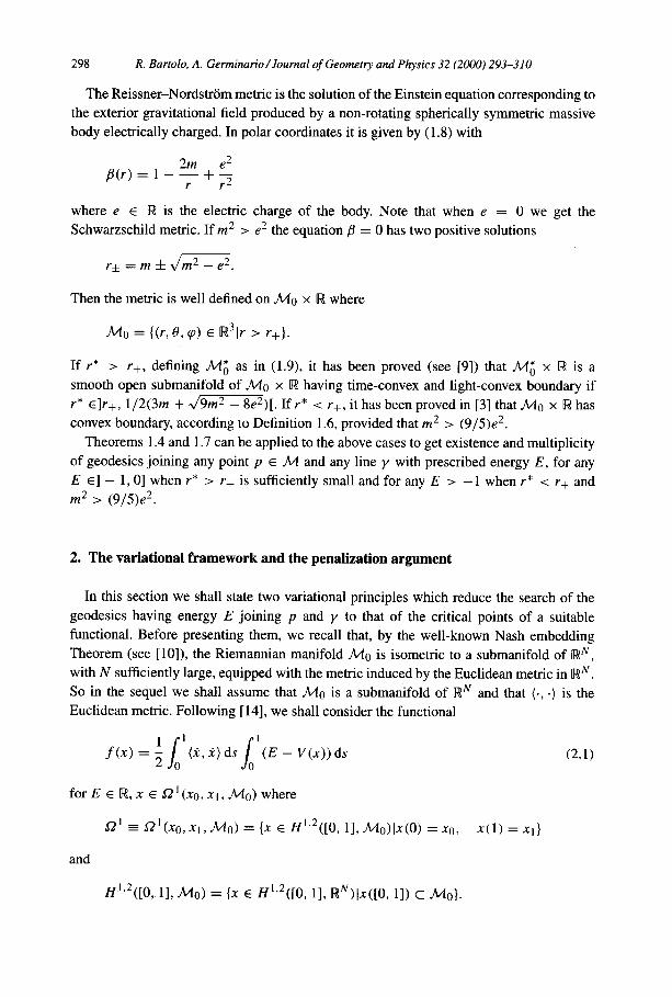
The Reissner-Nordstrom metric is the solution of the Einstein equation corresponding to the exterior gravitational field produced by a non-rotating spherically symmetric massive body electrically charged. In polar coordinates it is given by (1.8) with

b(r) = 1 - ? + $_

where e E R is the electric charge of the body. Note that when e = 0 we get the Schwarzschild metric. If m2 > e2 the equation ,!I = 0 has two positive solutions

Then the metric is well defined on Ma x R where

MO = I@, 8, YJ) E R31r =- r+]

If r* > r+, defining MT, as in (1.9), it has been proved (see [9]) that MT, x R is a smooth open submanifold of MO x I%! having time-convex and light-convex boundary if r* ~]r+, 1/2(3m + J9m2 - 8e2)[. If r* < r+, it has been proved in [3] that MO x [w has convex boundary, according to Definition 1.6, provided that m2 > (9/5)e2.

Theorems 1.4 and 1.7 can be applied to the above cases to get existence and multiplicity of geodesics joining any point p E M and any line y with prescribed energy E, for any E E] - 1, 0] when r* > r+ is sufficiently small and for any E > - 1 when r* -C r+ and m2 > (9/5)e2.

2. The variational framework and the penalization argument

In this section we shall state two variational principles which reduce the search of the geodesics having energy E joining p and y to that of the critical points of a suitable functional. Before presenting them, we recall that, by the well-known Nash embedding Theorem (see [lo]), the Riemannian manifold MO is isometric to a submanifold of RN, with N sufficiently large, equipped with the metric induced by the Euclidean metric in RN. So in the sequel we shall assume that MO is a submanifold of RN and that (., .) is the Euclidean metric. Following [ 141, we shall consider the functional

f(x) = ;l’(i.i)d$E - V(x))ds

forE E R,n E 52’(xo,x~,Mo) where

(2.1)

52’ = sZ’(xo,xt, MO) = {x E dg2([0, 11, Mo)lx(0) = x0, x(1) = xl)

and

ff1*2([0, 11, MO) = lx E H',2([0, 11, R'?Ix([O, 11) c Mol.

R. Bartolo, A. Germinario/Journal of Geometry and Physics 32 (2000) 293-310 299

It is well known that D’ is a Hilbert submanifold of H’,‘([O, 11, MO) whose tangent space at x E 52 ’ is given by

73’ = I< E H’.2(]0, 11, TMo)It(s) E Gc,,)Mo t(O) = 0 = t(1)).

The following proposition whose proof can be found in [ 1,121, allows the geodesics joining p and y to be found by studying the solutions with prescribed energy of a Lagrangian system on MO. This approach is different from the one previously used for this kind of problem (see the variational principle in [2]).

Proposition 2.1. Fix E E IR and let x : [0, a] + MO be a solution of

D,x = -VV(x), x(0) = x0, x(a) = x1, ;(i, i) + V(x) = E,

(2.2)

where V = - l/B. Then, set z = (x, t), with

s s

I(S) = Jz 1

~ dt, 0 B@(r))

(2.3)

z is a geodesic of energy E joining p and y. Vice-versa, consider a geodesic z = (x, t) of energy E joining p and y and such that p(x)i = 2/2. Then x is a solution of (2.2).

Now we can state the following variational principle for (2.2). For the proof see [ 1,141.

Proposition 2.2. Let V E C2(Mo, R) boundedfrom above and E E R, E > sup V. (i) Let x E a’ be a critical point off with f ( ) x > 0. Then y(s) = x(os), s E [O. h],

where

wz(x) = .&?F - V(x))ds

i&(-i-,k)ds ’ 0.4)

is a solution of (2.2). (ii) Let y be a solution of (2.2). Then x(s) = y(as), s E [0, l] is a critical point off on

52 ’ with f(x) > 0.

Hence, in order to prove Theorems 1.4 and 1.7, we have to look for the critical points of the functional f. Let us recall the well-known Palais-Smale condition.

Definition 2.3. Let (X, h) be a Riemannian manifold modelled on a Hilbert space and let F E C’(X, R). We say that F satisfies the Palais-Smale condition if every sequence (x,,)~~N such that

(F(x,))~~,,, is bounded (2.5)

and

llVF(x,)ll -+ 0, as m ---+ +cc (2.6)

300 R. Bartolo, A. Geminario/Journal of Geometry and Physics 32 (2000) 293-310

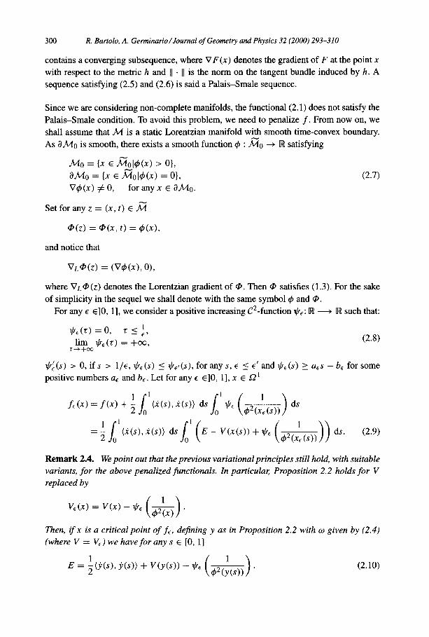
contains a converging subsequence, where V F (x) denotes the gradient of F at the point x with respect to the metric h and )] . 11 is the norm on the tangent bundle induced by h. A sequence satisfying (2.5) and (2.6) is said a Falais-Smale sequence.

Since we are considering non-complete manifolds, the functional (2.1) does not satisfy the Palais-Smale condition. To avoid this problem, we need to penalize f. From now on, we shall assume that M is a static Lorentzian manifold with smooth time-convex boundary. As ~Mo is smooth, there exists a smooth function 4 : 50 + R satisfying

MO = Ix E ~ol#(x) > 01, aMo = (x E &iolqW = 01, V@(x) # 09 for any x E aMo.

Setforanyz = (x,t) EM

Q(z) = @(X> t) = 4(x),

and notice that

(2.7)

VL@(Z) = (v+(x), O),

where Vr. Q,(z) denotes the Lorentzian gradient of 0. Then @ satisfies (1.3). For the sake of simplicity in the sequel we shall denote with the same symbol 4 and @.

For any E ~10, 11, we consider a positive increasing C2-function $<: R ---_, R such that:

$6(r) = 0, r i ;, l& $e(r) = +oo, (2.8)

$:(s) > 0, ifs > l/c, 9%(s) i Ilr8(s), f or any s, E 5 E’ and $< (s) 1 a,s - b, for some positive numbers a, and b,. Let for any E ~10, 11, x E a ’

fc(x> = f(x) + ; i’b.(s)> i.(s)) ds I’ $6

1 ’ =- 2 o (k(s), k(s)) ds

J E - V(x(s)) + @e

Remark 2.4. We point out that the previous variational principles still hold, with suitable variants, for the above penalized jimctionals. In particulal; Proposition 2.2 holds for V replaced by

Then, if x is a critical point off<, dejining y as in Proposition 2.2 with w given by (2.4) (where V = V,) we have for any s E [0, l]

E = ;(?;(s,, Y(s)) + V(Y(S)) - I++< c&d. (2.10)

R. Bartolo, A. Germinario/Journal of Geometry and Physics 32 (2000) 293-310 301

Lemma 2.5. Let E > sup V and@ E ~]0,1]. Let (x,),~N be a sequence in 0’ and K be a constant such that

.fc(xm) i K, for any m E N, (2.11)

inf(@(x,(s>)]s E [O, 11, m E N} > 0. (2.12)

Proof. By (2.11) it easily follows that the sequence (x,),~N is bounded in L*. Moreover, (2.11) and the Holder inequality imply that

Then (2.12) is a consequence of the following lemma, see e.g. [9]. 0

Lemma 2.6. Let (Xm)mEN be a sequence in R1 such that

s

I sup hn, a,) ds < foe meN 0

and let (s,)~~N in [0, l] be u sequence such that

m~~~wtz(s,)) = 0.

Then

(2.13)

(2.14)

(2.15)

Proposition 2.7. Assume that E > sup V. Then, (i) for any E ~10, l] andfor any c E Iw the sublevel

f:’ = Ix E fillf&) 5 c]

is a complete metric subspace of D ’ ; (ii) for any E ~10, 11, f6 satisjes the Palais-Smale condition.

Proof. Let (x,),e~ be a Cauchy sequence in f,‘, then it is a Cauchy sequence also in ZY’.*([O, 11, RN) and it converges to a curve x in H ‘**([O, I], RN). Since this convergence is also uniform, by Lemma 2.5 it results that x E Sz ’ and by the continuity of fC, we obtain the first part of the proposition. Now let (x,),~N be a Palais-Smale sequence; in particular it results that

(l’(&,im)ds)mEN isbounded. (2.16)

Then, up to a subsequence, we get the existence of ax E H’.*([O, 11, RN) such that

x, + x weakly in H’,2([0, 11, RN). (2.17)

302 R. Bartolo, A. Germinario/Journal of Geometry and Physics 32 (2000) 293-310

Arguing as in the first part of the proof, we get that x E S2 ‘. Using standard arguments, it can be proved that

x, + X strongly in H1,2([0, 11, RN). 17

Our next aim is to prove some a priori estimates on the critical points of the penalized functionals; in particular, we shall prove the following proposition.

Proposition 2.8. Let (x~)~~Io, 11 be a family ofcurves of 52’ such thatfor any e ~10, 11, x6 is a critical point of fC and let K E [w be a constant such that

f<(x<) i K, Ve ~10, 11. (2.18)

Then there exists an infmitesimal and decreasing sequence (em)mCN of numbers in IO, l] such that (x+,),~N strongly converges in H1,2([0, 11, RN) to a curve x E 52’ which is a critical point off.

Remark 2.9. It is easy to see that if(.~)~~]~, 1) is a family of criticalpoints of ft such that (2.18) holds, there exists a positive real number L 1 such that

FS;?, o’(. s x,,i,)ds = L1. (2.19)

Moreover; for any E ~10, 11, ifx E 52 ’ is a critical point of ft, then it satisfies the following equation:

A,(x)D,x + B,(x)VV(x) = -B,(x) V@(x), (2.20)

where

A<(x) = I

B,(x) = ; s

(i, k) ds. 0

According to Proposition 2.2, see also Remark 2.4, let us set

A,(x) o&x) = -.

B,(x)

To prove Proposition 2.8 some lemmas are needed.

Lemma 2.10. Let (x,),~Io,II be a family of curves of Q’ such thatfor any E ~10, 11, xc is a criticalpoint off<. Then, settingfor any E ~10, 11, s E [0, l/w,], z~(s) = (y<(s), t6(s)), where yt is given by Proposition 2.2 and

J s

t,(s) = 1/2 1

~ dr, 0 B(y,(r))

for any s E [0, l/0+] it results

(2.21)

(2.22)

R. Bartolo, A. Genninario/Joumal of Geometry and Physics 32 (2000) 293-310 303

Proof. Observing that for any s E [O, 11

;(i,(s), i<(S))(L) = $(j,(s), j<(S)) + V(Y,(S))

proof follows from Remark 2.4 and (2.10). 0

Remark 2.11. Consider the Riemannian metric on M given by

(t, OR = (6,t) +/%b2

for any z = (x, t) E M and [ = (c, s) E TIM. As H@ is a bilinearform

H#(z)K, 51 I c(Z)(cT t)R

for some positive constant c(Z).

Letx, E 52’ beacriticalpointof fc andletusset,foranyE ~10, 11,s E [0, 11:

h,(s) = 2 43(&(s)) +: L’iA ) (2.23)

see (2.20). The following estimate on the family (&)EE1o. t1 holds.

Lemma 2.12. There exists EO ~10, l] such that the family of functions (h,)tE~(),E,,~ is bounded in Loo([O, 11, W).

Proof. For any E > 0 we set g<(s) = 4(x,(s)), so g, is a C2-function on [0, 11. Let sc be a minimum point for g,. Since $< is convex, Q: is non-decreasing, so it results:

for any s E [0, 11, hence it is enough to prove that (h, (.s~))~~Io. 11 is bounded and to study the case in which

inf 4 (x, (se)) = 0. (2.24) CEIO. II

Let z,(s) = (y6(s), &(.s)) s E [0, l/w,], as in Lemma 2.10. As y<(s) = x,(o,s), where wz(x,) = A,(x,)/B,(x,), t< = s,(l/w,), is a minimum point for h,(s) = $(zc(s)) = @(y,(s)) on [O, l/we]. Now let us set, for any E ~10, l] , s E [O, l/we]:

It is easy to see that zr satisfies the equation

D,it = -P~(s)~L~J(z<)

and that & (s<) = p<(r<) for any 6 ~10, 11. Moreover by (2.24)

(2.25)

(2.26)

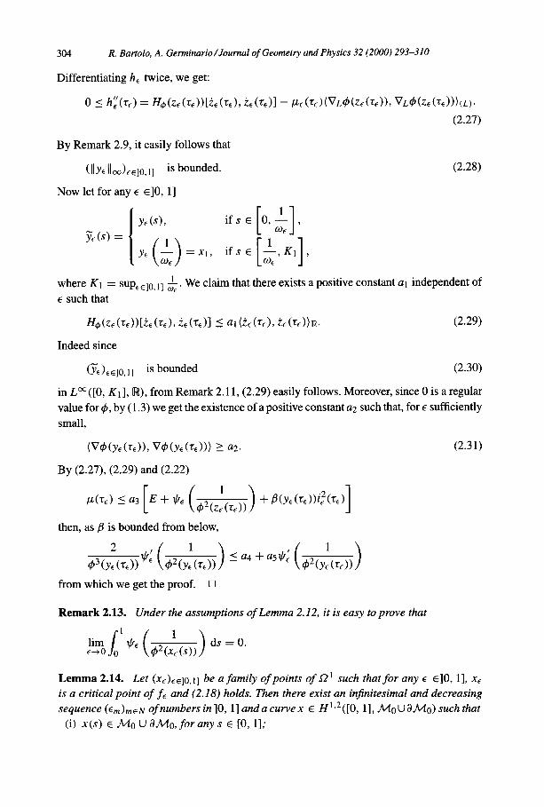
304 R. Bartolo, A. Genninario/Journal of Geometry and Physics 32 (2000) 293-310

Differentiating h, twice, we get:

0 I h:‘(q) = H&(tc))[i,(r,), i,(~>l - PE(G~E)(VL@(ZE(G)). VL~(~E(~~))~L)~ (2.27)

By Remark 2.9, it easily follows that

(IIY~~~~)~~~~,~~ is bounded.

Now let for any E ~10, 11

(2.28)

L 1

Y,(S), ifsE O,- ,

j;,(s) = [ 1 @

1 1 YE -

( > = XI, ifsE --,KI ,

WC [ 1 we

where K1 = SU~,~~~, r1 &. We claim that there exists a positive constant al independent of

E such that

H&(r,))[&(r<), i,(G)1 5 Qck(~~56)~ i,(G)h. (2.29)

Indeed since

(Y~)~~IO, 11 is bounded (2.30)

in Loo([O, Kl], W), from Remark 2.11, (2.29) easily follows. Moreover, since 0 is a regular value for $, by (1.3) we get the existence of a positive constant a2 such that, for E sufficiently small,

(V4(Y,(7,)), V$(Yc(G))) 2 a2. (2.31)

By (2.27), (2.29) and (2.22)

then, as jl is bounded from below,

from which we get the proof. 0

Remark 2.13. Under the assumptions of Lemma 2.12, it is easy to prove that

Ebjy @c ($2(x,(s))) ds = O. Lemma 2.14. Let (x~)~~Io,II be a family of points of Sz’ such that for any c ~10, 11, x6 is a critical point of fe and (2.18) holds. Then there exist an infinitesimal and decreasing sequence (E,),~N ofnumbersin]O, l] andacurvex E H1*2([0, 11, MoUaMo) such that

(i) x(s) E MO U aMo. for any s E [0, 11;

(ii) (iii)

R. Bartolo, A. Germinario/Joumal of Geometry and Physics 32 (2000) 293-310 305

b,,, )rn~N converges strongly to x in III’,~([O, 11, RN); there exists A. E L2([0, 11, I%), h(s) > 0 almost everywhere in [0, 11, h(s) = 0 if x(s) E MO, such thatfor any Jf E T,Q’(xo, XI, fro):

(2.32)

Proof. By Remark 2.9, there exists an infinitesimal and decreasing sequence (Cm)mER; of numbers in IO, l] and a curve x E H’s2([0, 11, RN) such that

x6, -+ x weakly in H’.2([0, I], RN). (2.33)

Since (x,,,)~~N converges to x also uniformly and MO U 8Mo is complete we have (i). The same arguments used to prove the strong convergence in Proposition 2.7, allow to get (ii). By Lemma 2.12, the sequence (&,,)mE~ is bounded, in particular, in L’([O, 11, [w), so there exists A E L2([0, 11, W) such that

&, -+ A weakly in L2([0, 11, R) (2.34)

and it results h non-negative almost everywhere. It is well known, see e.g. [9], that by (2.33), for any 6 E T,G!‘(xo, xl, Go), set for any m E N e,,,(s) = P(x,(s))[t], where, for any y E &, P(y) is the projection of RN on TV,&, it results that (cm)“&,! has a subsequence weakly convergent to t in iY’*2([0, I], RN). So, since for any m E N

0 = f:,, (xc,,, ) k,,, 1 = A<, (xc,, 1 s

’ k,, 3 kc,,, ) ds - &m (x,,n ) ’ WV (xc,,, 1, L, ) ds 0 s 0

s

1

-Benz (XEm ) h,,,(s)(VW,,), &m) ds, (2.35) 0

taking the limit, we get (iii). 0

Now let

H2,2([0, 11, rWN) = (x E H’.2([0, 11, RN)Jf is absolutely continuous,

x E L2([0, 11, RN>],

andletH2*2([0, 11, &)bethesubsetofH2,2([0, I], OBN)ofthecurvessuchthatx([O, 11) C GO. Integrating by parts (iii) of Lemma 2.14 as 6 E TX 0 ’ (x0, XI, GO) is arbitrary, it results that x E H2g2([0, 11, Go) is a weak solution of the equation

s

1 I (a, x) dsVV(x)

0 (E - V(x)) dsD,f + ;

s 0

s

I = -k(s) (i, i) dsV&(x).

0 (2.36)

306 R. Bartolo, A. Germinario/Joumal of Geometry and Physics 32 (2000) 293-310

Lemma 2.15. Let n as in Lemma 2.14. Let so E [0, l] such that x(sg) E MO. Then there exists a closed neighborhood J of SO such that h(s) = 0 for any s E J.

Proof. Since x(su) E MO and x is continuous, there exists a closed neighborhood J of so such that x(s) E MO for any s E J. As the sequence (~~,,,)~e,v uniformly converges to x, by (1.3), there exists u E N such that

d = inf{e5(x,,(s))]s E J, m p u} > 0.

By (2.8) for any m E N, m 1 v, such that E, < d2, we have

Then, taking the weak limit as m + 00 we get h(s) = 0, for any s E J. 0

Now we are ready to prove Proposition 2.8.

Proof of Proposition 2.8. Under our assumptions, by Lemma 2.14, there exists an infinitesi- mal anddecreasing sequence (~~)~e,v ofnumbers in IO, l] andacurvex E H2*2([0, 11, Go) with support in MO U aMo such that (ii) of Lemma 2.14 holds. Moreover (2.36) holds; we shall prove that the multiplier vanishes almost everywhere. Indeed, we know that h(s) = 0 if x(s) E MO; now let S ~10, 1[ such that x(S) E 8Mo and X(S) exists, then S is a minimum point of g(s) = 4(x(s)), so g’(S) = 0, g”(S) > 0. Arguing as in Lemma 2.10, we can consider z = (y, t) with y and t as in Proposition 2.2. Letting h(s) = $(z(s)) = @(y(s)), we shall call t the minimum point corresponding to S. So, differentiating twice, by (1.4), we get:

0 P h”(t) = &(z(S))[i(t), i(Gl + (VL$(Z(~)), &i(f))(~) 5 -P.(7)(vL#(z(~)), VL4(Z(f)))(L), (2.37)

where @ denotes the multiplier corresponding to z. Then by (iii) of Lemma 2.14 we obtain &) = 0 almost everywhere. Finally, we get z([O, A]) c M since z is a geodesic with energy E joining two points of M and aM is time-convex. 0

By the results of this section we get, for suitable E, the existence of a geodesic of energy E joining p and y.

Theorem 2.16. Let M = MO x R be a static Lorentzian manifold with smooth time- convex boundary such that MO U aMo is complete. Assume that there exist L, q > 0 such that (1.5) holds and let p = (x0,0) E M and v(s) = (xl, s) E M, s E R be such that p @ y(R). Then, for any E E] sup V, O[, there exists a geodesic of energy E joining p and y.

Proof. Since for any E ~]0,1] fe is bounded from below, satisfies the Palai-Smale con- dition and its sublevels are complete, ft attains its minimum at a curve x6 E 52 ’ . Moreover

R. Bartolo, A. Getminario/Joumal of Geometry and Physics 32 (2000) 293-310 301

it is easy to see that such family satisfies (2.18) for a certain K, so by Proposition 2.8, we get the existence of a critical point of f. By Proposition 2.1 and Proposition 2.2 the proof is complete. 0

3. Proof of Theorem 1.4

At first, we recall some definitions and results, see e.g. [ 131 and [9]

Definition 3.1. Let X be a topological space. Given a subspace A of X, the category of A in X, denoted with catx A, is the minimum number of closed and contractible subsets of X covering A; if A is not covered by a finite number of such subsets of X, we set catx A = +co.

Now we recall a min-max theorem due to Ljusternik and Schnirelmann.

Theorem 3.2. Let N be a Riemannian manifold and F a C’ -functional on N satisfying the Palais-Smale condition. Let us assume that N is complete or that every sublevel of F in N is complete. Set for any k E N

fx = (A c N[catNA 2 k},

ck = j$ si!F(x), .x

assume that rk is not empty and ck

For the following theorem see [.5].

(3.1)

E [w. Then ck is a critical value of F.

Theorem 3.3. Let N be a non-contractible Riemannian manifold and let x0, xl be two points of N. Then there exists a sequence (K,,,),,,~N of compact subsets in 52’(xo, XI, N) such that

,ly, catnl K, = +CQ.

We have pointed out that the functional f does not satisfy the Palais-Smale condition, nevertheless its sublevels have finite category. Indeed, the following proposition, whose proof is essentially contained in [9], holds.

Proposition 3.4. For any c E [w,

catlt,l f’ < +oo.

Proof of Theorem 1.4. Let us consider (Km)mE~ as in Theorem 3.3. Then, if we set for any m E N

r, = {A c G”Icat,lA 1. m},

308 R. Bartolo, A. Germinario/Joumal of Geometry and Physics 32 (2000) 293-310

we get r’ # 0. By Theorem 3.2, for any m E N, E ~10, 11, the values

cc,m = j$ SUP f<(x) m XEA

are well defined and are critical points of fC. Take now (II E R and set

fol = ]x E Q’lf(x) > a].

By Proposition 3.4, there exists m = m(cr) E N such that, for any A E r,

Anfo, #fl.

Hence, for any E ~10, 11, we obtain

By Proposition 2.8, since cx arbitrary, the thesis follows. Indeed we get the existence of a sequence (-x,),~N of critical points of f such that (~(x,)),~N diverges, so by using the variational principles stated in Section 2, we can consider the associated sequence

zm = (ym, GA, with

1 rp,y (z,) = tm

( > - dYrn>

s KJzX

for a suitable constant K > 0, from which (1.6) follows. 0

4. Proof of Theorem 1.7

Now we study the case in which M is a static Lorentzian manifold with non-smooth convex boundary. The variational principles stated in Section 2 still hold. Moreover, con- sidering @ as in Definition 1.6, we can penalize the functional f as in the smooth case. Using Lemma 2.6 and standard arguments, see also Proposition 2.7, the following proposition can be proved.

Proposition 4.1. Assume that E > sup V. Then, (i) for any ??~10, l] andfor any c E Iw the sublevel

f,” = Ix 6 Q’If&) 5 cl

is a complete metric subspace in D’; (ii) for any ??~10, 11, fC sutisjes the Paluis-Smale condition.

Let us observe that, arguing as in the proof of Theorem 2.16, we get the existence of a family (xC),e)u, 1) of critical points of fc such that (2.18) holds. The following lemma holds.

Lemma 4.2. Let (x6),,,, be a sequence of criticalpoints of f6 such that (2.18) holds. Then, there exists a positive constant 61, independent of E, such that

@(x,(s)) 2 61 for any s 6 LO, 11.

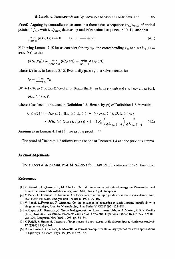
R. Bartolo, A. Germinario/Joumal of Geometry and Physics 32 (2000) 293-310 309

Proof. Arguing by contradiction, assume that there exists a sequence (~+,,)~~,v of critical points of fG,, with (E,,&~N decreasing and infinitesimal sequence in IO, 11, such that

min Wem(~)) + 0 as m-+oc. SC[O. 11

(4.1)

Following Lemma 2.10 let us consider for any xm, the corresponding zm and set h,(s) =

~(z,,,(s)) so that

where K 1 is as in Lemma 2.12. Eventually passing to a subsequence, let

to = ,:I, rm.

By (4.1), wegettheexistenceofp > 0 suchthatform largeenoughandr E [rc-p, SO+@]:

$(zm(r)) -=Z 6,

where 6 has been introduced in Definition 1.6. Hence, by (v) of Definition 1.6, it results

0 5 h;(r) = H,$(Zm(T))[im(t), i,(r)1 + (VL4(Zm(T))7 &&(~))(L,

Arguing as in Lemma 4.1 of [3], we get the proof. 0

The proof of Theorem 1.7 follows from the one of Theorem 1.4 and the previous lemma.

Acknowledgements

The authors wish to thank Prof. M. Sanchez for many helpful conversations on this topic.

References

[1] R. Bartolo, A. Germinario, M. Sanchez, Periodic trajectories with fixed energy on Riemannian and Lorentzian manifolds with boundary, Ann. Mat. Pura e Appl., to appear.

[2] V. Benci, D. Fortunato, F. Giannoni, On the existence of multiple geodesics in static space-times, Ann. Inst. Henri Poincart, Analyse non lit&ire 8 (1991) 79-102.

[3] V. Benci, D.Fortunato, F. Giannoni, On the existence of geodesics in static Lorentz manifolds with singular boundary, Ann. SC. Normale Sup. Pisa Serie IV XIX (1992) 255-289.

[4] A. Capozzi, D. Fortunato, C. Greco, Null geodesics on Lorentz manifolds, in: A. Marino, M.K.V. Murthy (Eds.), Nonlinear Variational Problems and Partial Differential Equations, Pitman Res. Notes in Math., vol. 320, Longman, New York, 1995, pp. 81-84.

[5] E. Fadell, S. Husseini, Category of loop spaces of open subsets in Euclidean Space, Nonlinear Analysis 17 (1991) 1153-1161.

[6] D. Fortunato, F. Giamroni, A. Masiello, A Fermat principle for stationary space-times with applications to light rays, J. Geom. Phys. 15 (1995) 159-188.

310 R. Bartolo, A. Germinario/Joumal of Geometry and Physics 32 (2000) 293-310

[7] F. Giannoni, A. Masiello, P. Piccione, A variational theory for light rays in stably causal Lorentzian manifolds: regularity and multiplicity results, Comm. Math. Phys. 187 (1997) 375415.

[8] F. Giannoni, A. Masiello, P. Piccione, A timelike extension of fermat’s principle in general relativity and applications, Calc. Var. 6 (1998) 263-283.

[9] A. Masiello, Variational methods in lorentzian geometry, Pitman Res. Notes in Math., vol. 309, London, 1994.

[lo] J. Nash, The embedding problem for Riemannian manifolds, Ann. Math. 63 (1956) 20-63. [I l] B. O’Neill, Semi-Riemannian Geometry with Applications to Relativity, Academic Press, New York,

London, 1983. [12] M. S&nchez, Geodesics in static space-times and T-periodic trajectories, Nonlinear Analysis 35 (1999)

677-686. [ 131 J.T. Schwartz, Nonlinear Functional Analysis, Gordon and Breach, New York, 1969. [ 141 E.W.C. Van Groesen, Analitycal mini-max methods for Hamiltonian brake orbits of prescribed energy,

J. Math. Anal. Appl. 132 (1988) 1-12.