Mobile Netw ApplDOI 10.1007/s11036-009-0181-6

GeoDTN+Nav: Geographic DTN Routing with NavigatorPrediction for Urban Vehicular Environments

Pei-Chun Cheng · Kevin C. Lee ·Mario Gerla · Jérôme Härri

© The Author(s) 2009. This article is published with open access at Springerlink.com

Abstract Position-based routing has proven to be wellsuited for highly dynamic environment such as Vehicu-lar Ad Hoc Networks (VANET) due to its simplic-ity. Greedy Perimeter Stateless Routing (GPSR) andGreedy Perimeter Coordinator Routing (GPCR) bothuse greedy algorithms to forward packets by selectingrelays with the best progress towards the destinationor use a recovery mode in case such solutions fail.These protocols could forward packets efficiently giventhat the underlying network is fully connected. How-ever, the dynamic nature of vehicular network, suchas vehicle density, traffic pattern, and radio obstaclescould create unconnected networks partitions. To this

This paper is an extended version of the one selected as oneof the best papers in ISVCS 2008.

The work is partially supported by the InternationalTechnology Alliance sponsored by the U.S. Army ResearchLaboratory and the U.K. Ministry of Defense underagreement number W911NF-06-3-0001, and partiallysupported by the state of Baden-Wurttemberg, TschiraFoundation, PTV AG and INIT AG to the research groupon Traffc Telematics.

P.-C. Cheng · K. C. Lee (B) · M. GerlaComputer Science Department, University of California,Los Angeles, CA 90095, USAe-mail: kclee@cs.ucla.edu

P.-C. Chenge-mail: pccheng@cs.ucla.edu

M. Gerlae-mail: gerla@cs.ucla.edu

J. HärriKarlsruhe Institute of Technology (KIT),76131 Karlsruhe, Germanye-mail: haerri@kit.edu

end, we propose GeoDTN+Nav, a hybrid geographicrouting solution enhancing the standard greedy and re-covery modes exploiting the vehicular mobility and on-board vehicular navigation systems to efficiently deliverpackets even in partitioned networks. GeoDTN+Navoutperforms standard geographic routing protocolssuch as GPSR and GPCR because it is able to estimatenetwork partitions and then improves partitions reach-ability by using a store-carry-forward procedure whennecessary. We propose a virtual navigation interface(VNI) to provide generalized route information to op-timize such forwarding procedure. We finally evaluatethe benefit of our approach first analytically and thenwith simulations. By using delay tolerant forwarding insparse networks, GeoDTN+Nav greatly increases thepacket delivery ratio of geographic routing protocolsand provides comparable routing delay to benchmarkDTN algorithms.

Keywords geographic routing ·delay tolerant network · navigation interface ·store-carry-forward · VANET

1 Introduction

Vehicular Ad Hoc Networks (VANET), a particularinstance of Mobile Ad Hoc Networks (MANET), area particular kind of networks, where vehicles or trans-portation infrastructures equipped with transmissioncapabilities are interconnected to form a network. Thetopology created by vehicles is usually very dynamicand significantly non uniformly distributed. In orderto transfer information on that kind of networks, stan-dards MANET routing algorithms are not appropriate.

Mobile Netw Appl

The other particularity of VANET is the availability ofnavigation systems, thanks to which each vehicle maybe aware of its geographic location as well as its neigh-bors’. A particular kind of routing approach, calledGeographic Routing becomes possible, where packetsare forwarded to destination simply by choosing a neigh-bor which is geographically closer to the destination.

Although geographic routing is a promising methodin VANET, it also has limitations. Due to the non uni-form topology distribution, a node may not be able tofind a neighbor closer to the destination than itself;a situation called a “local maximum” occurs. Severalrouting protocols have been proposed (GPSR [4],GPCR [9], VCLCR [7]) to solve this problem. GPSRintroduces a perimeter mode to extract packets fromlocal maxima by planarizing the network and forward-ing packets around the obstacle. This solution hasbeen proved to be suboptimal in VANET first as theplanarization procedure is complex and second as italso forces a packet to progress in small steps. GPCRsuppresses planarization by assuming that urban streetmaps naturally form planar graphs. Each road segmentis an edge of a planar graph while nodes at junctionsare vertices. Routing decisions are made only at junc-tions; between junctions, packets are simply forwardedto next junction. The limitation of GPCR is that itassumes that the junction nodes always exist. But inreality, it is not always true. When junction nodes aremissing, packets will be forwarded across junctions,causing possible routing loops. VCLCR attempts tosolve this problem by detecting loops and removingcross links whenever possible. It greatly increases thepacket delivery ratio compared to GPSR or GPCR.

Unfortunately, even if VCLCR can detect routingloops and remove cross links, packets can still bedropped due to network disconnection or partitions.Indeed, in case of sparse VANETs or when vehiclesin a VANET are significantly aggregated at junctions,network partitions occur and none of the previouslydescribed solution is able to deliver packets across par-titions. However, vehicles mobility patterns may helpto recover from this situation by letting a vehicle carrypackets to a different partition. If sufficient vehiclesare moving between network partitions, then packetscan be delivered even if the network is disconnected.This is the idea behind the concept of Delay Tol-erant Networks (DTN) [3]. DTN protocols such as[12, 13] employ such a store-carry-and-forward mecha-nism to forward packets yet at the cost of an increasedrouting delay.

Numbers of delay tolerant routing protocols exploit-ing different strategies to route packets have been de-veloped. GeOpps [8] takes advantage of the vehicles’

navigation system suggested routes to select vehiclesthat are likely to move closer to the final destinationof a packet. It calculates the shortest distance frompacket’s destination to the vehicles’ path, and estimatesthe arrival of time of a packet to destination. Duringthe travel of vehicles, if there is another vehicle thathas a shorter estimated arrival time, the packet willbe forwarded to that vehicle. The process repeats un-til the packet reaches destination. MoVe [6] uses themotion vector of a node to take forwarding decisions.The motion vector represents a node’s current movingdirection. MoVe chooses the neighbor which has theshortest distance to destination. The shortest distanceto destination is calculated as the distance from desti-nation to the extending line of the motion vector. Avariante is MoVe-Lookahead [6], which uses the nextwaypoint, i.e. points where vehicles change their direc-tions, instead motion vectors to calculate the shortestdistance.

All of these routing algorithms lack an integratedprotocol to combine both the efficient position-basedrouting for connected partitions and delay tolerant for-warding for routing between partitions. In this paper,we propose a complete solution as shown in Table 1,called GeoDTN+Nav, that includes the greedy mode,the perimeter mode, and the DTN mode. In order toknow when to use one of these modes, a network parti-tion detection method is proposed to evaluate for eachpacket the correct forwarding method to use in orderto guarantee a better packet delivery even in sparseor partitioned networks. We also introduce the VirtualNavigation Interface (VNI) which efficiently providesnavigator predictions in order to choose the best delaytolerant forwarders. We analytically and simulativelymeasure the performance of our solution and illustratehow it outperforms GPSR and GPCR and managesto transmit information when they both fail. We alsoshow the capability of GeoDTN+Nav using diverse andheterogenous information provided by VNI. The useof diverse navigational information greatly improvesthe packet delivery compared to single-metric DTNrouting protocols like GeOpps [8]. In GeoDTN+Nav,geographic routing is employed for efficient and fastrouting within network partitions, while DTN “data

Table 1 Packet delivery concept

Packet delivery Connected/dense Sparse networknetwork

Geo-routing Fast No delivery (dropped)DTN routing Slow SlowGeoDTN+Nav Fast Slow

Mobile Netw Appl

mules” are used to ensure correct delivery betweenpartitions yet at the cost of an increased delay.

The rest of the paper is organized as follows: InSection 3, we formally introduce the virtual navigationinterface model. Section 4 describes the GeoDTN+Navalgorithm and illustrate its properties. Section 5 pre-sents a simplified analytical model to evaluate theperformance of GeoDTN+Nav. Section 6 presentsthe synthetic and realistic simulative evaluation ofGeoDTN+Nav. Section 2 provides a short discussionof the current efforts in geo-routing and delay tolerantforwarding. Section 7 discusses ways to deliver packetsto moving vehicles as part of the future work. Finally,Section 8 concludes the paper.

2 Related work

We briefly describe two categories of routing proto-cols used in VANET, geographic routing and delay-tolerant routing since GeoDTN+Nav being a hybridapproach considering concepts from both categoriescannot be compared solely with protocols of one cate-gory. For each category, we present related work toGeoDTN+Nav.

2.1 Geographic routing

Greedy perimeter stateless routing The Greedy Perim-eter Stateless Routing (GPSR) [4] is a routing protocolthat uses the positions of wireless node and the destina-tion location of the packet to decide the forwardingdecision. In GPSR, intermediate nodes only main-tain the location of their neighbor nodes rather thanrouting metrics, which makes the protocol stateless.GPSR has two modes: greedy forwarding mode andperimeter mode.

In a network using GPSR as routing protocol, whenan intermediate node receives a packet, it will forwardthe packet to the neighbor that is geographically closestto the destination node. This approach is called greedyforwarding. If an intermediate has no other neighborscloser to the destination than itself, this intermediatenode is the local maximum node for this packet andthe packet will switch to the perimeter mode to recoverfrom the local maximum.

The idea of GPSR’s perimeter mode is to forwardpacket by right-hand rule with the starting vector con-straint. When a packet switches itself to the perimetermode at an intermediate node x, it first draws a virtualvector from x to destination node D. Node x thenforwards the packet to the first edge counterclockwiseabout x from the vector. (An edge here is defined as

a bi-direction feasible transmission pair between twowireless nodes.) Then GPSR always finds the nexthop by the right-hand rule—the next forwarding edgeshould be the first edge counterclockwise from the pre-vious edge without crossing the starting vector. Whena packet is forwarded to a node which is closer to Dthan x, it switches back to greedy forwarding mode.Otherwise, when it loops back to x, the packet willbe dropped.

The perimeter mode of GPSR must be applied on aplanar graph, or the crosslink may cause routing loops.GPSR proposes two schemes to construct a planargraph. However, issues such as obstacles and asymmet-ric radio range cause planar graphs unable to be formedcorrectly. Many later works have proposed geographicrouting without the requirement of planar graphs.

Greedy perimeter coordinator routing Two methodsare proposed in GPSR to construct planar graph: Rela-tive Neighborhood Graph (RNG) and Gabriel Graph(GG). However, it is impossible to construct a planargraph in VANET, because the network topology isalways changing. Each time when nodes move, a newplanar graph has to be constructed. Greedy PerimeterCoordinator Routing (GPCR) [9] solves the planariza-tion problem by exploiting the urban street map thatnaturally forms a planar graph. Each road segmentforms the edge in network topology, and the junctionsof roads form the vertices. In GPCR’s greedy mode, anode forwards packets until it reaches a node at a junc-tion. The junction node forwards packets by choosingone neighbor which has the shortest distance to desti-nation. In the perimeter mode, junction nodes forwardpackets to the next hop by applying right-hand rule.Non-junction nodes forward packets until it reaches ajunction node.

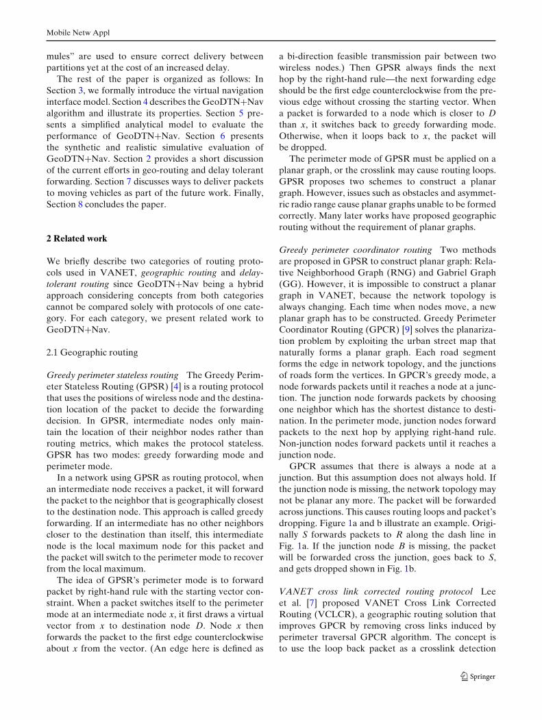
GPCR assumes that there is always a node at ajunction. But this assumption does not always hold. Ifthe junction node is missing, the network topology maynot be planar any more. The packet will be forwardedacross junctions. This causes routing loops and packet’sdropping. Figure 1a and b illustrate an example. Origi-nally S forwards packets to R along the dash line inFig. 1a. If the junction node B is missing, the packetwill be forwarded cross the junction, goes back to S,and gets dropped shown in Fig. 1b.

VANET cross link corrected routing protocol Leeet al. [7] proposed VANET Cross Link CorrectedRouting (VCLCR), a geographic routing solution thatimproves GPCR by removing cross links induced byperimeter traversal GPCR algorithm. The concept isto use the loop back packet as a crosslink detection

Mobile Netw Appl

R

S

B

B

R

S

(a) Simplied street map (no (b) Junction B is empty (twocross links). cross links).

Fig. 1 Cross-link causes routing loops (a, b)

probe. When a packet is forwarded by perimeter mode,it records the path information in the packet. Whenthe packet routes back to the perimeter mode’s startingpoint, it checks the path it traverses and sees if there isa routing loop and cross links.

More specifically, when a node receives a packet anddiscovers that there is a loop, it checks the traversalhistory and sees if it has traversed through any crosslink. If not, it indicates there is no available path tothe destination and the packet will be dropped. Other-wise, the packet will be forwarded again by right-handrule. In addition, one of the neighboring links that iscrossed and only traversed once will be removed. Thereason that links traversed twice will not be removed isbecause it may disconnect the graph [5]. This cross-link-removal procedure is on-demand and the overhead issmall. When a packet in the perimeter mode is for-warded to any node that is closer to the destinationnode than the perimeter mode’s starting node, thepacket will switch back to greedy forwarding mode andreset its path information.

When the packet is forwarding on a path withoutcross link, VCLCR performs the same as GPCR. Byeliminating loops in packets paths, VCLCR increasesthe packet delivery rate and also reduces failed hopscompared to GPCR.

2.2 Delay-Tolerant Network (DTN) routing

This section presents only the DTN routing approachesrelevant to GeoDTN+Nav. Readers can refer to [15]for an overview of the state of the art DTN routingprotocols for different types of delay tolerant networks.

Mobile Relay Protocol (MRP) MRP [11] is a relay-based approach that is used in conjunction with tradi-tional ad hoc routing protocol. A node would engage intraditional routing until a route to the destination is un-obtainable. It then performs controlled local broadcastto its immediate neighbors. All nodes that receive thebroadcast store the packet and enter into the relayingmode. Such nodes carry the packet until their buffer isfull. When that happens, the relay-nodes would chooseto relay the packet to a single random neighbor. Similarto MRP, GeoDTN+Nav combines traditional ad hocrouting and DTN routing. However, a GeoDTN+Navnode does not broadcast to its local neighbors in theDTN mode. Furthermore, the node constantly seeksthe best neighbor to deliver to the destination sinceholding packets until the buffer is full or until therelay node meets the destination prolong the end-to-end delay.

Context Aware Routing (CAR) CAR [10] integratessynchronous and asynchronous mechanisms for mes-sage delivery. A synchronous message delivery mech-anism is characterized by a contemporaneous pathbetween the current node and the destination; whereas,an asynchronous message delivery mechanism does nothave such a path. The concept is similar to the hybridapproach adopted by GeoDTN+Nav where a nodeswitches to the DTN mode when its scoring functionindicates network disconnectivity. More importantly,during asynchronous message delivery, a node relays toanother node with the highest probability of reachingthe destination by the evaluation and prediction ofthe context information. An utility function similar toGeoDTN+Nav’s scoring function is used. However,CAR did consider weights of each contextual parame-ter (e.g., rate change of connectivity, battery life, etc.)dynamically. Since CAR uses DSDV for traditional adhoc routing, it introduces prediction to reduce the over-head of dissemination of routing table. CAR providesanother framework of utilizing the contextual infor-mation with dynamic-weight consideration geared to-wards sensor networks and prediction geared towardsproactive routing.

Model Based Routing (MBR) Chen et al. [1] presentsa model based routing that takes advantage of thepredictable node moments along a highway. Authorshave verified the hypothesis that the motion of vehicleson a highway can contribute to successful messagedelivery, provided that messages can be relayed andstored temporarily at moving nodes while waiting foropportunities to be forwarded further. As a result,

Mobile Netw Appl

GeoDTN+Nav takes node movements into consider-ation when computing the next forwarding node in theDTN mode.

GeOpps GeOpps [8] is a delay tolerant routing algo-rithm that exploits the availability of information froma navigation system (NS). Such navigation systemincludes a GPS device, maps, and the function to cal-culate a suggested route from current position to a re-quested destination. In GeOpps, each vehicle equippedwith an navigation system communicates with oneanother and obtains information to perform efficientand accurate route computation.

A NS is assumed to have the ability to calculatethe route to a given destination and to estimate therequired time to a given destination. When a vehiclewants to deliver a data packet, it broadcasts the des-tination of it. The one-hop neighbors of the packetholder will calculate the “Nearest Point” (NP). Sinceevery vehicle using NS has a suggested path, the NP isthe location that is the location on the path which isgeographically closest to the destination. For example,in Fig. 2, paths a, b and c are the different suggestedpaths of three vehicles. Their NPs to the destination Dis marked as N Pa, N Pb, and N Pc. The weakness ofthe approach is that the scheme assumes all vehicleshave a navigation system and the navigation systemprovides the same transmission format and content.The assumption is not true in reality. As a natural

Fig. 2 GeOpps Neighbor Selection, where their routes are eval-uated with respect to the potential “Nearest Poin” (NPx) to thedestination D

Fig. 3 GeOpps Problem,where node A is chosenas DTN mule whereas ageo-routing would haveused the connected graphand selected node B fora faster progress

consequence of the design, GeOpps does not utilizeheterogenous information from devices other than thenavigation system and misses opportunities of findinga better forwarder. Furthermore, since it is a DTNrouting protocol and packets tend to be held by nodeswhose NP is closer to the destination than another nodewhose NP is further yet it is on the connected path tothe destination, thus, nodes generally experience higherdelay in GeOpps than in GeoDTN+Nav. For example,Fig. 3 shows a two-lane road segment with traffic inopposite directions. A sender node S is sending packetsto a curb-side destination D. Among S’s neighbors Aand B, A has the closest NP to the destination D.Thus, in GeOpps, the packet would be delegated toA. Since no other nodes have closer NP to the desti-nation, the packets would remain stored at A and onlydelivered to the destination when A meets D. On thecontrary, in GeoDTN+Nav, the packet would be firstforwarded using geographic routing and successfullydelivered at D since there is a connected path from Sto D. Given that radio propagation is much faster thanvehicle movement, we can expect that GeoDTN+Navhas lower latency in other similar scenarios.

3 Virtual navigation interface framework

The goal of the Virtual Navigation Interface (VNI) isto help discover neighboring vehicles that can deliverpackets in partitioned networks. Without any priorinformation, randomly choosing a neighbor to carry apacket might not be appropriate because this neighbormight move farther away from the destination. Yet,with external knowledge of neighbors’ path or destina-tion information, we could make a better decision.

Mobile Netw Appl

In [8], GeOpps assumes that vehicles are equippedwith navigation systems that contain geographical loca-tions. Hence it makes carrier decision based on whichneighbor can deliver the packet quicker/closer to itsdestination. This assumption might be valid since moreand more cars are equipped with on-board naviga-tion systems. In addition, modern applications, such asroute suggestion based on real-time traffic and prox-imity based advertisement, may encourage the deploy-ment of navigation systems. However, this assumptionneglects the heterogeneity of vehicles. Indeed, althoughthe content of GPS information has been standard-ized, the content and transmission format of navi-gation information is not and may differ betweendifferent classes of vehicles, if these latter vehicles areeven equipped with such devices. For example, roadidentification can differ from one navigation system toanother. The map encoding of a road on one navigationsystem may define a road as one separated by junctions;whereas, the map encoding of a road on another naviga-tion system may define a road naturally from the nameof the road.

In GeoDTN+Nav, we adopt a more relaxed andgeneralized assumption and provide a unified frame-work for the different kinds of navigation informationavailable. We assume that every car is equipped witha Virtual Navigation Interface (VNI). We describe theassumption and model of VNI in the following sections.

3.1 Vehicle mobility categories

In this section, we present a scenario that motivates theidea of virtual navigation interface. As Fig. 4 shows, dif-

ferent kinds of vehicles together create a vehicular adhoc network. These vehicles move based on differentpatterns:

– Bus, train: These vehicles’ movement is strictly re-stricted by a predefined route. For a given bus, itsdestination, path to the destination, and scheduleare given in advance. For these vehicles, they do notrequire navigation systems, but they would movebased on a deterministic route,

– Taxi, Van pool: Unlike previous ones, these vehi-cles do not move along a fixed route. However,no matter how different the routes are, they wouldeventually arrive at a predefined destination. Forexample, a taxi driver may dynamically choose adifferent path to avoid traffic, but he should stilldrive passengers to their destination,

– Vehicles equipped with Navigation Systems: Pri-vately owned vehicles might be equipped with navi-gation systems. These vehicles are expected tofollow the route suggested by navigation systemsbecause navigation systems usually suggest shortestroutes, or simply because drivers may not knowthe route to their destinations. However, it is alsopossible that drivers do not follow the suggestedroute or they may change the destination duringtheir travel. Therefore, these vehicles introduceextra uncertainties in its movement pattern,

– Vehicles not equipped with Navigation Systems:Privately owned vehicles also might not beequipped with navigation systems, and thereforethey are not capable of providing their route infor-mation. However, these vehicles still do not move

Fig. 4 Categories ofvehicular route patternand VNI example

Food Mart

w/ NavigationVNI : (Path, 25%)

w/o NavigationVNI : (?, 0%)

w/ NavigationVNI : (Dest, 75%)

TaxiVNI : (Dest, 100%)

BusVNI : (Path, 100%)

Mobile Netw Appl

randomly. For example, vehicles are expected tomaintain their direction along a road before theyarrive at the next junction. It is not likely thatvehicles would move back and forth irrationally.

Based on vehicles movement pattern discussed above,we categorize vehicles into four broad categories:

1. Deterministic (Fixed) Route: Vehicles movestrictly along preconfigured routes. These vehicleswill not deviate away from their routes. Also, themoving direction of vehicles can be derived fromtheir routes,

2. Deterministic (Fixed) Destination: Vehicles movestrictly toward a preconfigured destination. How-ever, it is possible that vehicles take different routesto reach the destination. A coarse-grain movingdirection can also be obtained,

3. Probabilistic (Expected) Route / Destination: Vehi-cles may move based on suggested routes or desti-nations. They are allowed to change their route ordestination discretionarily,

4. Unknown: Vehicles could not provide informationabout their route, but they do not move randomlyeither.

Categories of vehicles and examples are summarizedin Table 2.

3.2 Virtual Navigation Interface (VNI) design

We have already discussed different categories of ve-hicles in the previous section. In order to provide aconsistent and generalized view of different vehicles inour routing decision, we assume VNI is installed onevery vehicle. VNI is a lightweight wrapper interfacethat interacts with underlying vehicular components. Itprovides two kinds of primitive information:

1. Route_info: Route_info represents the vehicle’sroute information. Note that route informationmay either consist of detailed path, destination, orthe direction of vehicles, depending on the types

Table 2 Categories of vehicular route pattern

Categories Examples

Deterministic (fixed) route Metro bus, metro train,campus shuttle

Deterministic (fixed) destination Taxi, van poolProbabilistic (expected) Navigation system

route/destination guided vehiclesUnknown Non-random movement

underlying data sources. As in Fig. 5, VNI mightbe able to retrieve detailed path information froma navigation system while it may only retrievevehicle’s direction from an Event Data Recorder(EDR). In addition, VNI can also retrieve pre-configured route information.

2. Confidence: Confidence indicates the probabilitythat the vehicle’s movement would abide by thegiven route information. More specifically, confi-dence with 0% means that the vehicle move com-pletely in random while confidence with 100%means that the vehicle move strictly based on itsroute information. This confidence information canbe configured or derived from vehicles’ movementhistory.

For example, in Fig. 4, we installed VNI on everyvehicle:

– VNI on buses would broadcast two-tuple informa-tion (Path, 100%) because buses move determinis-tically along its preconfigured route.

– VNI on taxis would broadcast (Dest, 100%) be-cause taxis move deterministically toward itsdestination.

– VNI on vehicles with navigation systems wouldbroadcast (Path/Dest, P%) depending on what in-formation the VNI can obtain from the underlyingnavigation system.

– VNI on vehicles without navigation systems mightbroadcast (?, 0%) because VNI cannot obtainenough route information, or it might broadcast(Dir, P%), if VNI is able to estimate vehicles’ mov-ing direction.

Based on the unified information provided by VNI,every vehicle now can collect navigation information

VNI

EDRHard-codedPath/Destination

NavigationSystem

NAV_INFO(Path | Dest | Direction)CONFIDENCE

•

•

Fig. 5 Virtual navigation interface

Mobile Netw Appl

from its neighbors and make routing decision accord-ingly. Note that this generic information advertised byVNI is independent from our GeoDTN+Nav protocol.It can also be used by other routing protocols servingdifferent purposes. However, in this paper, we focuson using information provided by VNI to choose aneighbor which can potentially carry packets acrossdisconnected networks.

4 GeoDTN+Nav algorithm

Traditionally, geo-routing routes packets in two modes:the first mode is the greedy mode, and the second modeis the perimeter mode. In greedy mode, a packet is for-warded to destination greedily by choosing a neighborwhich has a bigger progress to destination among all theneighbors. However, due to obstacles the packet canarrive at a local maximum where there is no neighborcloser to the destination than itself. In this case, theperimeter mode is applied to extract packets from localmaxima and to eventually return to the greedy mode.After a planarization process, packets are forwardedaround the obstacle towards destination. In this way,the packet delivery is guaranteed as long as the networkis connected.

However, the assumption that the network is con-nected may not always be true. Due to the mobile char-acteristics of VANET, it is common that the networkis disconnected or partitioned, particularly in sparsenetworks. The greedy and perimeter modes are notsufficient in VANET. Therefore, we introduce the thirdmode: DTN (Delay Tolerate Network) mode, whichcan deliver packets even if the network is disconnectedor partitioned by taking advantage of the mobilityof vehicles in VANET. Unlike the common beliefthat mobility harms routing in VANET, we specificallycount on it in this work to improve routing.

In short, packets are forwarded first forwarded in thegreedy mode, and then by the perimeter mode whena packet hits a local maximum. If the perimeter modealso fails, it finally switches to the DTN mode and relieson mobility to deliver packets. Figure 6 illustrates thetransition diagram between these three modes.

Greedy Perimeter DTN

Progress Found

Local

maximum

Disconnected

Network

Fig. 6 Switch between greedy, perimeter, and DTN mode

Two questions arise in this scheme: Exactly whenshould we switch to DTN mode, and when to switchback to the greedy mode. For the former, we will usea cost function and a threshold related to a networkpartition detection and to the quality of nodes mobilitypattern between partitions. For the latter, similar to therecovery mode, we will return to the greedy mode whena relay with better progress than the one that triggeredthe DTN mode is found. We will discuss the details inSection 4.3.

4.1 Restricted greedy forwarding

In GeoDTN+Nav, the default greedy forwarding strat-egy is the same as the restrictive greedy forwarding inGPCR, where packets are always forwarded betweenjunction nodes as junctions are the only places wherea node can make significant routing decisions. This re-mains true even if a current forwarding node can greed-ily forward packets beyond a junction. At junctions,a greedy decision is made to determine which roaddirection should be taken that can bring the maximumprogress towards the destination. If a local maximumis reached, the recovery mode, called the perimeterforwarding, is used.

4.2 Perimeter forwarding

In GeoDTN+Nav, the default recovery mode is thesame as VCLCR’s. The goal of VCLCR in perimeterforwarding is to detect and remove cross links createdby the lack of junction nodes to improve packet de-livery. For GeoDTN+Nav, in order to support delaytolerant forwarding, we piggyback the following extrafields in data packets as shown in Fig. 7:

1. DTN_Flag: the DTN_flag indicates whether or notthis packet can be forwarded by delay tolerantmode. Applications that do not require on-timedelivery can enable this flag to improve packetdeliver probability.

Fig. 7 Packet format

. . .

Data

DTN_Flag

DTN_Timeout

Hops

Mobile Netw Appl

2. DTN_Timeout: Applications specify packets’ toler-ated delay. Based on this information, nodes bufferand carry DTN packets can flush packets that arealready expired or decide which packet to deletebased on buffer management policy.

3. Hop_Count: The field records the number of hopsthat a packet has been forwarded in the perimetermode.GeoDTN+Nav uses this information to determineif the network is disconnected. This field can bereplaced or augmented if future work adopts othermeans to measure network connectivity.

The basic idea behind GeoDTN+Nav is that inthe perimeter forwarding mode, nodes keep suspectingwhether the network is disconnected based on howmany hops the packet has traveled in the perimetermode. Every node also monitors its neighbors’ navi-gation information. Based on the connectivity and navi-gation information, a switch score is calculated for eachneighbor. A packet would be switched to DTN modeonly when the switch score is beyond a certain prede-fined threshold and the DTN_flag is set.

For all neighbors, if no switch score is beyond thethreshold, the packet would be forwarded based onconventional perimeter forwarding and increment thehops by one.

4.3 DTN forwarding

With DTN forwarding, the first question to address iswhen we should switch to DTN mode. Two factors needto be considered: network disconnections and deliveryquality of nodes storing a packet. Determining networkdisconnectivity is not an easy task; in fact, there is noway to know whether the network is connected or notunless we have the complete information of networktopology. Moreover, even if we have the complete net-work topology information, any decision is only validat the time of the evaluation because the topology ischanging all the time. Thus, what we can do is to takea good guess. We propose to base this decision on thehop count, as an increasing hop count in the perimetermode could mean the network is partitioned.

The delivery quality of nodes carrying a packet is thesecond criterion to determine whether we should useDTN forwarding or not. If there is a good neighbor thathas a mobility pattern that will bring the packet closerto destination, we rely on it to deliver the packet. By agood neighbor, we mean a neighbor which has a path,destination, or direction towards the destination withhigh confidence. For example, a bus may have paths inNVI because its route is well-known, and may have high

confidence because it seldom changes such route. A taximay not transmit its path but its destination because itonly knows the destination where customers want to go,and the confidence associated to that destination is lowas real traffic condition may alter it.

Network disconnectivity and the delivery qualityonly are not enough to define a good neighbor. We alsohave to consider the neighbor’ moving direction. Forexample, a bus may have good delivery quality becauseit has a fixed route closer to destination but it is movingaway from it, which makes it a less favored relay tocarry a packet.

Combined the three factors, we derive the “scorefunction” S as follows:

S(Ni) = αP(h) × βQ(Ni) × γ Dir(Ni) (1)

where:

S(Ni) : Switching score of Ni

P(h) : Probability that the network is disconnected(range from 0 to 1)

Q(Ni) : Delivery quality of Ni in DTN mode(range from 0 to 1)

Dir(Ni) : Direction of Ni (range from 0 to 1)α, β, γ : System parametersNi : a neighbor of current node ih : hop counts that the packet has traversed in

the perimeter mode.

The function P(h) represents the probability that thenetwork is disconnected, as measured by hop counts.The larger the hop counts, the higher the probabilitythat the network is disconnected. We use Algorithm Pto calculate function P(h):

Algorithm PInput: Current hop count h, first edge traversed in the

perimeter mode e0Output: Probability that the network is disconnected1. nextHop ← perimeter forwarding by right-hand

rule from current node2. nextEdge ← current node to nextHop3. if nextEdge equals e04. then return 15. else return max(0,h−hmin)

hmax−hmin

In Algorithm P, hmax is the maximum hops for whichwe assume the network is connected. After this hopcount, P(h) equals to 1, which means the network isdisconnected. In our algorithm, hmax equals TTL. hmin

is the minimum hop counts that we will switch to DTNmode, i.e., we will only apply DTN forwarding afterthe packet has been forwarded more than hmin. Thereason for this is that the perimeter forwarding mode is

Mobile Netw Appl

more efficient than relying on mobile vehicles to deliverpackets. We therefore want to further try several hopsin the perimeter mode before switching to DTN mode.If a packet goes back to the point where it enteredthe perimeter mode (i.e., e0), Algorithm P will return1 because we simply assume that the network is parti-tioned. The relationship between hop counts and P(h)

is illustrated in Fig. 8:The function Q(Ni) represents the delivery quality

of neighbor Ni. We use Algorithm Q to compute thedelivery quality of each neighbor:

Algorithm QInput: Neighbor’s location (nl), neighbor’s confidence

(c), the destination (dest), the node that enters theperimeter mode (L f )

Output: Neighbor’s delivery quality ∈ R

1. D ← Dist(dest, L f )

2. d ← Dist(dest, nl)3. return (max(0,D−d)

D )c

In Algorithm Q, D is the distance between the des-tination and the location of the node that switchedto the perimeter mode. d is the distance between thedestination and the location information Nav-info ofneighbors broadcasted in beacon packets. If Nav-infocontains the path, then d is the distance from packet’sdestination to the closest road segment on this path.If Nav-info contains the neighbor’s destination, then dis the distance from packet’s destination to neighbor’sdestination. If Nav-info contains the direction, then dis the perpendicular distance from packet’s destinationto the extending line of the direction. For example, inFig. 9, the packet is now at node C. There are threeneighbors of current node, N1, N2 and N3. For N1,d=d1. For N2, d=d2. For N3, d=d2. Using AlgorithmQ, we obtain the delivery quality of each node.

As mentioned before, Q(Ni) may not be enough todefine a “good” neighbor; we also need to consider the

Fig. 8 Function P(h)

Fig. 9 Calculate Q(Ni)

moving direction. For example, in Fig. 9, for currentnode C, neighbor N1 has a path which has shortestdistance to destination. N1 is definitely a good choiceto forward packet in comparison to N2 and N3 in thiscase. But what if N1 is moving away from the des-tination at that time? Obviously it is not a good choiceto carry the packet. It may be better to choose a neigh-bor that is moving toward the destination rather thanmoving away. Therefore, we add the third function,Dir(Ni), in our score function:

Algorithm DirInput: Neighbor’s direction (ndr), the destination (dest),

the current node’s location (curLoc)Output: Neighbor’s direction quality ∈ R

1. θ ← the angle formed by the vector formed by ndrand the vector formed by dest and curLoc

2. if θ equals 03. then return 14. else return 1

abs(θ)

Here is the complete algorithm using all of the threemodes:

1. Everynodeperiodicallybroadcast two-tuplenaviga-tion information by VNI: (Nav-info, Confidence).

2. A packet is forwarded in the greedy mode, until itreaches a local maximum.

3. Then it switches to the perimeter mode and recordits own location e0 and its dest in the packet header.

Mobile Netw Appl

4. At each hop in the perimeter mode, do thefollowing:

(a) Use P(h) to calculate the probability of net-work disconnectivity.

(b) Use Q(Ni) to calculate the delivery quality ofeach of its neighbors as well as itself.

(c) Use Dir(Ni) to calculate the direction qualityof each neighbor.

(d) Calculate the global score for each node byusing Eq. 1.

(e) If one of the scores is greater than Sthresh, for-ward the packet to the respective node andswitch to DTN mode. The packet will bestored and carried by that node until it canswitch to the greedy mode. If there are multi-ple nodes that have greater scores than Sthresh,choose the node with highest score and for-ward the packet to it.

5. Increase the hop count. If the hop count reaches theTTL and there is no node with a score greater thanSthresh, drop the packet.

We have described an architecture that integratesthree modes (greedy, perimeter, DTN) in VANET inorder of delivery for sparse or partitioned networks.The “score function” here is an example that takes intoaccount of the network disconnectivity and deliveryquality of nodes carrying a packet. A better functioncan be derived from a careful analysis of traffic patternsand forwarding policy, which we let to future work. Wedescribe how we can efficiently set Sthresh in Section 5.

Note that, in GeoDTN+Nav, each node makes in-telligent decision based on the navigation informationwhich may not always be reliable. For example, evenbuses with fixed routes might detour to another routebecause of temporary road construction. However,notice that GeoDTN+Nav only exploits DTN forward-ing to recover network separation. A detoured vehiclemight carry packets to another connected network.Still, it is true that a detoured vehicle would strictlymove away from the destination so the packets haveto be eventually dropped. In this case, VNI wouldautomatically decrease this vehicle’s confidence value,which in turn makes this vehicle less favorable in thefuture DTN forwarding.

Lastly, we would like to emphasize that Geo-DTN+Nav is a distributed routing protocol, whichcan not guarantee the packet delivery. Depending onapplication requirements, upper layer protocols mayimplement their own mechanisms to acknowledgeend-to-end packet delivery. However, because of the

dynamic and evolving nature of vehicle networks, webelieve that GeoDTN+Nav is more suitable for con-nectionless message-based applications.

4.4 GeoDTN+Nav routing with VNI examples

After having described the VNI and the GeoDTN+Navrouting protocol, we now demonstrate their joint func-tionalities in two examples. We emphasize that themain purpose of switching from the perimeter mode toDTN mode is to virtually connect network partitionsand improve the delivery ratio, while switching fromDTN mode back to greedy is to improve delivery delayin connected partitions. For simplicity, we assume allpackets in our examples are already in the perimetermode and each node has already collected navigationinformation broadcasted by the VNI installed on itsneighbors.

4.4.1 Example 1: greedy to DTN

Assume weight parameters α, β, and γ are 1, and thethreshold Sthresh is 0.25. Also suppose that a packet hastraversed 8 hops in the perimeter mode up to node A.Node A has three neighbors, N1, N2, and N3. While thepacket arrives at node A, node A calculates the proba-bility of network disconnectivity by applying AlgorithmP and obtains P(8) = 0.4. Note that Algorithm P de-pends only on the hop counts that has been traversed inthe perimeter mode. At the same time, node A calcu-lates the delivery quality of its neighbors, also includingitself, in order to know if they could bring the packet tothe targeted network partition in DTN mode. It finallycomputes the “score function” S by multiplying P(h),Q(Ni), and Dir(Ni). At this time, none of its neighborsincluding itself has a higher score than Sthresh, so thepacket will remain in the perimeter mode to the nexthop. The above process repeats in node B, but now twoneighbors N2 and N3 have greater scores than Sthresh.Node B therefore switches to DTN mode, and choosesthe neighbor with the greatest score to carry the packet,node N2 in this case. N2 will buffer the packet until itreaches a point where it can switch back to the greedymode. Once it has reached that a point, the packetis forwarded to destination in the greedy mode again(Fig. 10).

4.4.2 Example 2: DTN to greedy

The second example, depicted in Fig. 11, illustrates thecondition for a node to switch from DTN mode to thegreedy mode. In this example, a packet first hit the local

Mobile Netw Appl

A

N1

N2

N3

B

N1

N2

N3

Q(NB) = 0.4

S(NB) = 0.2

P(B) = 0.5

Q(N1) = 0.1

S(N1) = 0.01

Q(N2) = 0.7

S(N2) = 0.35

Q(N3) = 0.6

S(N3) = 0.30

Q(NA) = 0.2

S(NA) = 0.08

P(A) = 0.4

Q(N2) = 0

S(N2) = 0

Q(N1) = 0.1

S(N1) = P(A) *

Q(N1) = 0.04

Q(N3) = 0.6

S(N3) = 0.24

Fig. 10 Routing example 1

maximum at point e0 where it switched to the perimetermode, before switching to DTN mode at node A. NodeA periodically checks on the packets in its buffer todecide whether there is a packet that can be forwardedagain in the greedy mode. In order to switch a packet’sforwarding mode back to greedy, Node A needs tofind a neighbor closer to the destination than the nodee0 where the initial local maximum was. As node Amoves to a point B, it detects that its distance to Destis smaller than the distance from e0 to Dest. Therefore,if a neighbor is located at that point, node A is able toswitch back to the greedy mode. If there is not such aneighbor, the packet will stay in Node A until it findsan applicable neighbor to forward packets, as it shouldnever switch back to greedy until it has reached the net-work partition possibly containing the destination node.

Fig. 11 Routing example 2

5 Parameters analytical evaluation

In Section 4, the algorithm for GeoDTN+Nav has beenproposed in order to improve packet delivery in sparseor partitioned networks for delay tolerant applications.Due to the large set of parameters, the performance ofGeoDTN+Nav may be hard to evaluate. This sectionproposes to study the proper settings for weight valuesand utility functions through an analytical model. Fordense and connected networks, greedy forwarding isable to efficiently deliver packets with low delay. Onthe contrary, for sparse or partitioned networks, it hasa high chance to fail and must switch to the perime-ter mode. If the perimeter mode designed by GPCRcannot successfully return to greedy, then we have theoption to switch to the DTN mode. This action howevertrades an improved delivery ratio for a significantlyincreased delivery delay. So, when tuning the settingsfor GeoDTN+Nav, we need to consider the applicationrequirements between delivery ratio and it respectivedelay. Table 3 displays the notation of our analysis.

In Section 4.3, Q(Nx) is introduced as the deliveryquality function for neighboring node after x hops, P(x)

is introduced as the probability of a disconnect networkafter a packet is forwarded for x hops, and Sthresh is thethreshold of scoring function to switch to DTN mode.These values together with weight parameters are thecontrollable setting for GeoDTN+Nav. They are usedto calculate Tx, which is the probability of switching toDTN mode after x hops.

The other variable Gx is defined as follows: When apacket is forwarded in the perimeter mode at xth hop,the probability that it switches to the greedy mode atnext hop is Gx and the probability that it remains inthe perimeter mode is 1 − Gx. Here we assume thatthis variable is obtained by simulation or real networkexperiment. By definition it is clear that

∞∑

i=1

{Gi

i−1∏

x=0

(1 − Gx)

}

Table 3 Notation in analytical model

Gx The probability of switching to the greedy mode afterx hops in the perimeter mode

NRx The expected number of type R neighboring nodes

after x hops in the perimeter mode.P(x) The probability that network is disconnected after

x hops.Q(Nx) The delivery quality function for traffic type R in

DTN modePx

Q(k) The probability mass function for Q(Nx) = kSthresh The threshold of switching to DTN

Mobile Netw Appl

is the probability that a packet can switch back tothe greedy mode after it enters the perimeter mode.Here, G0 = 0; that is, the probability of switching tothe greedy mode after x hops in the perimeter modeis 0. Intuitively, G0 = 0 says if a node has not tried toforward in the perimeter mode, it should try at leastone hop before considering switching to the greedymode. Since the inability to switch back to the greedymode means the network is either disconnected, or thepacket loops in the perimeter mode, the probabilitythat network is disconnected is at most

1 −∞∑

i=1

{Gi

i−1∏

x=0

(1 − Gx)

}.

Another variable that can be parameterized by mea-suring topology is NR

x . NRx stands for the expected

number of type R nodes that can be used for DTNmode when a packet is traversed in the perimeter modeon xth hop. Each type R represents different kinds ofvehicular category, such as taxis, buses, trains, or cars.Note that NR

x includes the node that currently holds thepacket, because if the packet owner itself finds out thatthe threshold is exceeded, it will change to DTN modeas well.

The definition of Tx is similar to Gx. When a packetis on its xth hop in the perimeter mode, it has a Tx

probability to switch to DTN mode on itself and anyof its neighboring nodes. For a type R node, if theforwarding packet is switched to DTN mode at thisnode, this node must satisfy the condition:

Sthresh ≤ αP(x)βQ(Nx)γ Dir(Ni).

Furthermore, it is reasonable to assume that Dir(Ni) isa uniform distribution between 0 to 1. Therefore, afterx hops, the probability that none of the neighboringnodes in type R satisfies this constraint is:

F Rx (Sthresh) =

(∫ 1

0

∫ Sthresh/αβγ zP(x)

0Px

Q(y)dydz

)NRx

Therefore, Tx can be written as follows:

Tx = 1 −∏

∀R

F Rx (Sthresh)

F Rx represents the probability that all type R nodes

within the delivery range of a current packet locationdo not have their scoring function S exceeding thethreshold forcing the packet to stay in the perimetermode.

Figure 12 demonstrates our framework about thisanalytical model. When a packet is forwarded in theperimeter mode, it has three choices. If any of itsneighbors is closer to destination than the starting pointin the perimeter mode, it will switch to greedy mode; ifany of its neighbor or itself exceeds the DTN threshold,it will switch to DTN mode; if none of the previous casehappens, it will remain in the perimeter mode. Given Tx

and Gx, the probability that a packet can successfullyexit the perimeter mode in x hops is:

G1 + (1 − G1)T1 + (1 − G1)(1 − T1)G2 + . . .

+ Gx

x−1∏

i=1

(1 − Gi)(1 − Ti)

+ Tx

[x−1∏

i=1

(1 − Gi)(1 − Ti)

](1 − Gx)

= 1 −x∏

n=1

(1 − Gn)(1 − Tn)

Furthermore, the probability that a packet switchesto the greedy mode in x hops is the odd terms of theequation, which is:

x∑

k=1

Gk Ik,

while:

Ik ={∏k−1

i=1 (1 − Gi)(1 − Ti), k > 1, k ∈ N

1, k = 1

Fig. 12 Markov Chain for theperimeter mode forwarding

Mobile Netw Appl

Similarly, the probability that a packet switches to DTNmode in x hops is the even terms of the equation,which is:

x∑

k=1

(1 − Gx)Tx Ix,

This model allows us to predict the probability thata packet will switch to DTN whenever it enters theperimeter mode.

To understand how DTN affects the average packetlatency, suppose that the hop-wise delivery delay inDTN mode is Dd, while that of the joint greedy andperimeter mode is Dg. The total average delay ofpacket delivery becomes:

x∑

k=1

Gx Ix Dg +x∑

k=1

(1 − Gx)Tx Ix Dd

Figures 13 and 14 illustrate the PDR vs. latencytradeoff as a function of the probability of switchingto DTN Tx, where the probability of switching to thegreedy mode Gx is fixed for each x, where Dg = 5,Gx = 0.1 and where a packet is dropped after 16 hops.As depicted on Fig. 13, the packet delivery ratio in-creases when the probability to switch to DTN goesup, if the application only requires a minimum packetdelivery ratio, it can be mapped directly to the probabil-ity to switch to DTN mode. Similarly, Fig. 14 providesan upper bound for the probability to switch to DTNwhen there is a maximum average delay constraint. Inthe above example, if the packet wishes to have 90%delivery ratio and a delay less than 400, the probabilityof switching to DTN should be set between 0.1 and 0.4by adjusting the threshold.

The next step is therefore to be able to compute athreshold satisfying the probability bounds. If a packet

0.7

0.8

0.9

1

0 0.2 0.4 0.6 0.8 1

Packet Delivery Ratio

T (Prob. of Switch to DTN)

PDR

Fig. 13 Probability vs. PDR

0

50

100

150

200

250

300

350

400

450

500

0 0.2 0.4 0.6 0.8 1

Latency (unit)

T (Prob. of Switch to DTN)

Latency (DTN Delay=500)Latency (DTN Delay=50 )Latency (DTN Delay=5 )

Fig. 14 Probability vs. latency

in the perimeter mode should switch to DTN for aprobability ranging from a to b , we have:

Tx = a < 1 −∏

∀R

F Rx (Sthresh) < b .

Thus,

1 − b <∏

∀R

F Rx (Sthresh) < 1 − a.

which leads to:∏

∀R

F Rx (m)

=∏

∀R

(∫ 1

0

∫ mk/z

0Px

Q(y)dydz

)NRx

=[(∫ mk

0Px

Q(y)dy

)−

∫ 1

0zPx

Q(mk/z)(−mk/z2)

]NRx

=[(∫ mk

0Px

Q(y)dy

)+

∫ 1

0mkPx

Q(mk/z)/zdz

]NRx

given k = 1/(αβγ P(x))

In conclusion, in order to have Tx bounded betweena and b , the threshold bound satisfies:

1 − b <

[(∫ mk

0Px

Q(y)dy

)

+∫ 1

0mkPx

Q(mk/z)/zdz

]NRx

< 1 − a

Figure 14 demonstrates another aspect of our ana-lytical model. Suppose there are three different types ofR nodes, and each of them has different DTN delay,Dd of 5, 50, 500, respectively. If the network application

Mobile Netw Appl

wishes to have a latency lower than 200 s with DTNdelay = 500, the probability of switching to DTN shouldbe 0.5. Moreover, if the DTN delay is 50 or 5, the packetcan always be delivered within 200 s. In this case thepacket delivery ratio becomes the only constraint thatis of concern. Once the probability of switching to DTNis obtained, Sthresh can be calculated by the methodmentioned above.

6 Performance evaluation

In this section, we are going to evaluate the perfor-mance of GeoDTN+Nav in two different scenarios: asynthetic one that aims at illustrating the concept ofGeoDTN+Nav and a realistic one that consists of areal urban map and realistic vehicular mobility. Table 4indicates the parameters we used in our simulations.

GeoDTN+Nav is compared against a randomizedDTN routing scheme [14], Rand − DT N. RandDTNworks as follows. At each beacon interval, a nodeforwards the packet it is carrying with probability p.When p = 0, RandDTN is reduced to direct trans-mission scheme where packets reach the destinationonly when the source node meets the destination node.When p = 1, a node always considers its neighbors toforward the packet. To avoid the packet from beingforwarded to any node, thus reducing progress towardsthe destination, we modify RandDTN so that the nodewould forward to its neighbor whose final destinationis closest to the destination of the packet. If such aneighbor does not exist, the node would simply storeand carry the packet until the next beacon interval.Moreover, in this paper, we set p = 0.5 for generality.

6.1 Synthetic scenario

We evaluate GeoDTN+Nav on a synthetic topologyto show it is able to improve packet delivery ratio by

Table 4 Simulation parameters

Parameter Value

Network simulator Qualnet 3.95Mobility simulator VanetMobisimCBR rate 64 Bytes/s802.11b rate 2 Mbps802.11b transmission power 15.0 dBmTX range 300 mAvg vehicle speed 50 km/hSimulation runs 30Confidence interval 95%Propagation Free space with inter-road

radio blocking model

Fig. 15 Synthetic topology

delay tolerant forwarding. In Fig. 15, nodes are placedso that they create two separate partitions. Obstaclesare placed between different road segments if they donot share the same horizontal or vertical coordinates.The length of each edge is 300 m, and the transmissionrange is 300 m. According to the topology, each packetsent from the source to the destination will reach a localmaximum and switch to the perimeter mode.

We place ‘Bus’ nodes at location A. ‘Bus’ nodesmove towards location B at a speed of 50 km/h. Wemanipulate the number of bus nodes as well as theirdeparture pattern in order to study the virtual con-nectivity between the two partitions. More precisely,we compare two departure patterns: a uniform pattern,in which a bus departure time is uniformly distributedthroughout the whole simulation time; and the Randompattern, in which each bus node randomly departs.

Simulations are ran with constant bit rate UDPtraffic with packet size of 64 bytes and compareGeoDTN+Nav with GPCR and RandDTN in packetdelivery ratio, latency, and hop count. For brevity, weonly show results of RandDTN for random departure.We set α = β = γ = 1. Based on the topology, packetsare transferred from one partition to the next by buses.Therefore, the delay experienced in the DTN mode isthe time it takes for a bus to arrive from one end of thepartition to another. We set Dd = 450 s.1 Furthermore,because the end-to-end latency is mostly attributed tothe delay in the DTN mode, it is set to Dd of 450 s. Wealso configure the probability of switching to the DTNmode to approximately 90%. Based on these valuesand according to our study in Section 5, the parameterSthresh is computed to be 0.1. Note that this value ofSthresh will also be used in the rest of this paper as wewould like to keep a similar DTN latency. The resultsof the synthetic scenario are depicted in Fig. 16.

1Since bus arrival varies depending on its departure pattern—random or uniform, Dd ranges anywhere from 150 s to 450 s.Dd is set to 450 s conservatively.

Mobile Netw Appl

0

0.2

0.4

0.6

0.8

1

5 10 15 20 25 30 35 40

Packet Delivery Ratio

Number of 'Bus' Nodes

0

0.1

5 10 15

(a) PDR

0

50

100

150

200

250

5 10 15 20 25 30 35 40

Latency (sec)

Number of 'Bus' Nodes

0

0.1

20 25 30

(b) Latency

0

5

10

15

20

25

5 10 15 20 25 30 35 40

Number of Hops

Number of 'Bus' Nodes

(c) Hop count

Fig. 16 Performance evaluation for the synthetic scenario (a–c)

In Fig. 16a, for uniform departure configuration,when the number of ‘Bus’ nodes is small and due tothe two network partitions, GPCR cannot deliver anypacket to the destination. However, GeoDTN+Nav

can achieve over 90% delivery ratio because pack-ets are carried by ‘Bus’ nodes between the differentpartitioned. As the number of ‘Bus’ nodes increases,GeoDTN+Nav obviously maintains a steady highpacket delivery ratio. On the contrary, GPCR has asharp PDR jump with between 20 and 25 nodes. Thereason is that the increasing number of ‘Bus’ nodes uni-formly spread over the edge AB eventually reconnectsthe two partitions and allows GPCR to successfullydeliver packets.

Similarly to uniform departure, GPCR is also notable to deliver any packet to the destination for the ran-dom departure configuration when the number of ‘Bus’nodes is small. On the contrary, GeoDTN+Nav canstill achieve around 80% delivery ratio. As ‘Bus’ nodesrandomly depart, there is a chance that not a single‘Bus’ node is available when GeoDTN+Nav needs it,which explains the 10% drop in delivery ratio betweenthe uniform and random departures. For GPCR, dueto random ‘Bus’ node departures, even an increasingnumber of ‘Bus’ nodes is never able to fully reconnectthe two partitions. It yet increases the probability tofind such configuration and explains the linear increaseof the GPCR delivery ratio with the number of ‘Bus’nodes. Note that RandDTN can also achieve over 60%delivery ratio. This is because, in this simple syntheticnetwork configuration, there is sufficiently high proba-bility for source nodes to meet ‘Bus’ nodes, which canhelp deliver packets to the destination.

Now considering the second metric set, Fig. 16band c show the average number of hops and latency adelivered packet travels. We may clearly see the trade-off with GeoDTN+Nav’s high packet delivery ratio, asthe number of hops and delivery delay are significantlyhigher. We however argue that the hop count andlatency of GPCR remains steadily low as it can onlydeliver packets when the network is connected. Whenthe number of ‘Bus’ nodes increases, the probabilitythat a packet can be delivered by GeoDTN+Nav butsolely based on the greedy mode also increases. There-fore, the hop count and the latency of packet deliverydecrease accordingly. Last, we can also see that Rand-DTN has higher latency. This is because RandDTN is apure DTN forwarding protocol which relies on nodes’physical movement to carry packets. This is expected tobe much slower than wireless communication.

6.2 Realistic scenario

In this particular experiment setup, realistic vehicularmobility traces have been generated using the Intel-ligent Driver Model with Intersection Management(IDM-IM) by VanetMobiSim [2], an open source and

Mobile Netw Appl

freely available realistic vehicular traffic generator fornetwork simulators. The mobility scheme is based ona sequence of activities (home, work, shopping, etc..)described by a relative transition probability matrix.The unified transmission range is 300 m. The urbantopology employed in this paper is a realistic 1500 mby 4000 m Oakland area from U.S. Census Bureau’sTopologically Integrated Geographic Encoding andReferencing (TIGER) database. All intersections arecontrolled by stop signs and all road segments containspeed limitations. Unless specified differently, all roadshave a single lane and a speed limit of 15 m/s (54 km/h).

We generate mobility traces for 50 nodes and intro-duce extra ‘Bus’ nodes. We manipulate the number ofbus nodes as well as their departure patterns. In eachsimulation, 20 random source nodes send data to a fixeddestination node using constant bit rate (CBR), a UDP-based packet generation application. To emulate radiopropagation in urban area, blocking radio obstacleshave been placed between different road segments ifthey do not share the same horizontal or vertical coor-dinates. In each experiment, we compare GPSR, GPCRand GeoDTN+Nav for the following metrics: 1) packetdelivery ratio (PDR), 2) latency, and 3) hop count. Wealso show in the figures the 95% confidence interval.

Initially, because the node density is low and theconnectivity is limited by obstacles therefore creatinga large number of network partitions, the packet de-livery ratio is very low for all protocols. This ‘realistic’scenario is more challenging than the ‘synthetic’ onefor GeoDTN+Nav, as ‘Bus’ nodes do not specificallyconnect two partitions and source-destination pairs arerandomly distributed. In Fig. 17a, as the number ofbuses increases, GeoDTN+Nav’s PDR increases ac-cordingly, first because nodes have a higher proba-bility to meet and delegate packets to ‘Bus’ nodes,but also as ‘Bus’ nodes have a higher chance to con-nect the corresponding partitions. However, withouta DTN mode, GPCR and GPSR remain unable toefficiently transport packets in such a partitioned net-work. We may also see in Fig. 17a that the uniformdeparture pattern also yields to a better PDR than therandom one.

However, unlike the synthetic experiment describedin the previous section, GPSR’s and GPCR’s PDRremain low even though the number of buses increases.For random source-destination pairs, the relatively lownumber of ‘Bus’ nodes is not sufficient to connect thedifferent partitions. In fact, as it may be observed inFig. 17c, GPSR and GPCR only successfully deliverpackets when the source and destination nodes areone hop away, which also results in low latency. InFig. 17b and c, as the number of buses increases,

0

0.05

0.1

0.15

0.2

0.25

0.3

0.35

0.4

0.45

5 10 15 20 25 30 35 40

Packet Delivery Ratio

Number of 'Bus' Nodes

Optimal(RAND)GPSR/GPCR(RAND)

GeoDTN+NAV(RAND)Optimal(UNIM)

GPSR/GPCR(UNIM)GeoDTN+NAV(UNIM)

RandDTN 0

0.1

5 10 15

(a) PDR

0

50

100

150

200

250

300

350

5 10 15 20 25 30 35 40

Latency (sec)

Number of 'Bus' Nodes

Optimal(RAND)GPSR/GPCR(RAND)

GeoDTN+NAV(RAND)Optimal(UNIM)

GPSR/GPCR(UNIM)GeoDTN+NAV(UNIM)

RandDTN 0

0.05

0.1

5 10 15

(b) Latency

0

5

10

15

20

25

5 10 15 20 25 30 35 40

Number of Hops

Number of 'Bus' Nodes

Optimal(RAND)GPSR/GPCR(RAND)

GeoDTN+NAV(RAND)Optimal(UNIM)

GPSR/GPCR(UNIM)GeoDTN+NAV(UNIM)

RandDTN

(c) Hop count

Fig. 17 Performance evaluation for the realistic scenario (a–c)

GeoDTN+Nav’s hop count and latency increase.This is GeoDTN+Nav’s fundamental tradeoff betweenpackets’ forwarding latency and delivery ratio.

Last, note that RandDTN achieves slightly betterPDR and lower latency than GeoDTN+Nav. This is

Mobile Netw Appl

because of the intelligent feature of GeoDTN+Nav:whenever the packet is carried across partitioned net-work, GeoDTN+Nav would try to switch back to geo-graphic routing. However, in such a sparse network,GeoDTN+Nav is likely to fall back to DTN modeagain, which increases the latency and might alsodecrease the PDR. However, owing to the dynamicand evolving nature of vehicular networks, we expectthat this hybrid geo-rouing and DTN forwarding na-ture of GeoDTN+Nav could yield better performancein general.

6.2.1 Benchmarking with optimal routing protocol

A unique feature of GeoDTN+Nav is its hybridrouting feature. Based on the “score function”,GeoDTN+Nav make intelligent decisions on switch-ing between position-based routing and delay tolerantrouting. Hence, the performance of GeoDTN+Navhighly depends on the correctness of the score func-tion. In this section, we further evaluate GeoDTN+Navby benchmarking it with an optimal unicast routingprotocol.

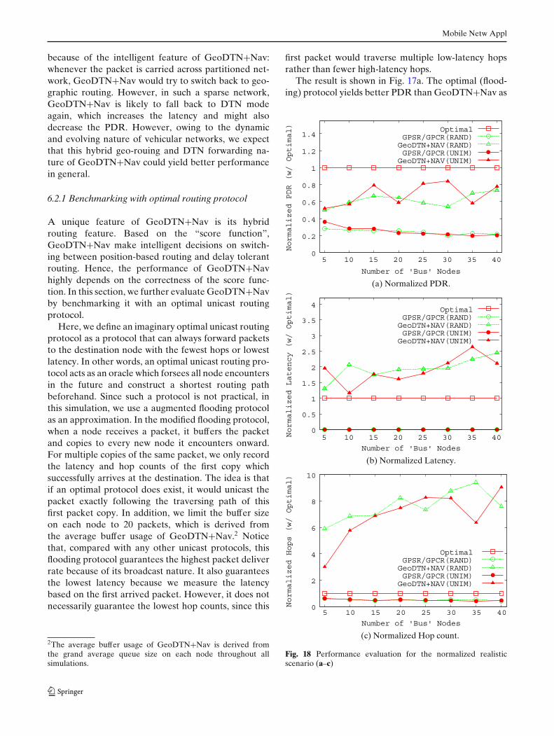
Here, we define an imaginary optimal unicast routingprotocol as a protocol that can always forward packetsto the destination node with the fewest hops or lowestlatency. In other words, an optimal unicast routing pro-tocol acts as an oracle which forsees all node encountersin the future and construct a shortest routing pathbeforehand. Since such a protocol is not practical, inthis simulation, we use a augmented flooding protocolas an approximation. In the modified flooding protocol,when a node receives a packet, it buffers the packetand copies to every new node it encounters onward.For multiple copies of the same packet, we only recordthe latency and hop counts of the first copy whichsuccessfully arrives at the destination. The idea is thatif an optimal protocol does exist, it would unicast thepacket exactly following the traversing path of thisfirst packet copy. In addition, we limit the buffer sizeon each node to 20 packets, which is derived fromthe average buffer usage of GeoDTN+Nav.2 Noticethat, compared with any other unicast protocols, thisflooding protocol guarantees the highest packet deliverrate because of its broadcast nature. It also guaranteesthe lowest latency because we measure the latencybased on the first arrived packet. However, it does notnecessarily guarantee the lowest hop counts, since this

2The average buffer usage of GeoDTN+Nav is derived fromthe grand average queue size on each node throughout allsimulations.

first packet would traverse multiple low-latency hopsrather than fewer high-latency hops.

The result is shown in Fig. 17a. The optimal (flood-ing) protocol yields better PDR than GeoDTN+Nav as

0

0.2

0.4

0.6

0.8

1

1.2

1.4

5 10 15 20 25 30 35 40

Normalized PDR (w/ Optimal)

Number of 'Bus' Nodes

OptimalGPSR/GPCR(RAND)GeoDTN+NAV(RAND)GPSR/GPCR(UNIM)GeoDTN+NAV(UNIM)

(a) Normalized PDR.

0

0.5

1

1.5

2

2.5

3

3.5

4

5 10 15 20 25 30 35 40Normalized Latency (w/ Optimal)

Number of 'Bus' Nodes

OptimalGPSR/GPCR(RAND)GeoDTN+NAV(RAND)GPSR/GPCR(UNIM)GeoDTN+NAV(UNIM)

(b) Normalized Latency.

0

2

4

6

8

10

5 10 15 20 25 30 35 40

Normalized Hops (w/ Optimal)

Number of 'Bus' Nodes

OptimalGPSR/GPCR(RAND)GeoDTN+NAV(RAND)GPSR/GPCR(UNIM)GeoDTN+NAV(UNIM)

(c) Normalized Hop count.

Fig. 18 Performance evaluation for the normalized realisticscenario (a–c)

Mobile Netw Appl

Table 5 Summary of normalized performance evaluation withrespect to “optimal routing”

Protocols Min Max

GeoDTN+Nav 50% 84%GPSR/GPCR 19% 36%

expected. In fact, we can take the result of the floodingprotocol as the upper bound of any unicast routing pro-tocols under the same configuration. Figure 18a showsthe PDR normalized with the PDR of the floodingprotocol. We can see that GeoDTN+Nav can achieveup to 80% of the highest possible PDR, as opposed toGPSR/GPCR, which only achieves around 30%. Thedownward trend of GPSR/GPCR’s normalized PDRreflects the fact that the increasing number of buseshelps flooding and GeoDTN+Nav but not enough tohelp GPSR/GPCR. The normalized performance issummarized in Table 5.

Figures 17b and 18b show the actual and nor-malized latency. Notice that the deliver latency ofGeoDTN+Nav is twice as large as the optimal latency.This is because whenever a node in GeoDTN+Navmakes a wrong switching decision, it might miss the busnode and has to wait for the next encounter of anotherbus node, which inadvertently increases the end-to-endlatency.

Finally, Figs. 17c and 18c show the actual and nor-malized hop count. Both GPSR and GPCR possesslower hop count and latency than the optimal proto-col because most of the successful delivery for GPSRand GPCR are one hop away. The optimal routing’shigher PDR verifies this claim: packets that have tobe delivered cross partitions are simply dropped byGPSR and GPCR; whereas, the optimal routing wouldstore the same packets and continue broadcasting themuntil they reach their destination. However, the opti-mal routing’s latency and hop count are lower thanGeoDTN+Nav’s as GeoDTN+Nav packets will haveto travel for more hops before switching to DTN mode.This is because we use a simple scoring function toguide the mode change in GeoDTN+Nav. The scoringfunction can be improved to choose a better neighborsor to remain longer in DTN mode, thereby reducingthe number of hops or latency. We leave this tunableparameter as future work.

6.2.2 Heterogeneity

In this section, we introduce ‘Taxi’ nodes as well as‘Bus’ nodes. We fix the total number of “Data Mules”(Buses and Taxis). We first let all data mules be taxis,then we gradually replace taxis with bus nodes by

5-node increment up to 40 bus nodes and 0 taxi nodes.For taxi nodes, the VNI only broadcasts its destinationcoordinates. When there are only taxi nodes in the

0

0.05

0.1

0.15

0.2

0.25

0.3

0.35

0.4

0 0.2 0.4 0.6 0.8 1

Packet Delivery Ratio

Percent of 'Bus' Nodes

Optimal(RAND)GeoDTN+NAV(RAND)

Optimal(UNIM)GeoDTN+NAV(UNIM)

(a) PDR.

0

50

100

150

200

250

300

350

0 0.2 0.4 0.6 0.8 1

Latency (sec)

Percent of 'Bus' Nodes

Optimal(RAND)GeoDTN+NAV(RAND)

Optimal(UNIM)GeoDTN+NAV(UNIM)

(b) Latency.

0

5

10

15

20

25

0 0.2 0.4 0.6 0.8 1

Number of Hops

Percent of 'Bus' Nodes

Optimal(RAND)GeoDTN+NAV(RAND)

Optimal(UNIM)GeoDTN+NAV(UNIM)

(c) Hop count.

Fig. 19 Performance evaluation for the heterogenous scenario.X-axis indicates the percent of ‘bus’ nodes out of 40 data mules.x-axis = 0 may emulate GeOpps while larger x-axis values showthe benefits of GeoDTN+Nav

Mobile Netw Appl

network, GeoDTN+Nav approximates the behavior ofGeOpps given that the routes of taxis are known. Asthere are more buses in the network, GeoDTN+Navenjoys the diversity of options in forwarding packets.Figure 19a shows that as the number of buses increases,the PDR increases, indicating the delivery quality ofbuses is better than the taxis’. By further investigation,we found that even though some taxi’s destinationis near the packet’s destination, from the networkingpoint of view, the taxi’s destination and the packet’sdestination are disconnected. There are also taxis whichmay have a destination that is far from the packet’s des-tination even though they pass the packet’s destination.By only looking at the destination coordinates may leadto suboptimal decisions.

The results shed light on the advantage of Geo-DTN+Nav over GeOpps which relies only on taxis todeliver packets3 and yields lower PDR of 13% and12% than GeoDTN+Nav’s in random and uniform busdeparture, respectively. By incorporating simply a fewbus nodes, GeoDTN+Nav is able to use both types ofvehicles to deliver packets successfully.

7 Future work

7.1 Moving destination

Moving destination is a common issue in geographicrouting, especially for vehicular networks in whichnodes move with comparatively higher speed. For rout-ing protocols that only have knowledge of the posi-tional information, a best effort solution to movingdestination is either to drop the packet or query thelatest destination’s location and forward the packettowards destination’s latest location again. A moreaggressive solution may even allow immediate nodes toquery and update the location of packet’s destination.However, these solutions inadvertently introduce addi-tional query delay and network traffic.

In GeoDTN+Nav, we propose solutions exploit-ing the navigation information. Two approaches areconsidered:

1. Passive Tracking: In this approach, packets are firstforwarded to the destination location. If the des-tination node has moved away, these packets are

3GeOpps cannot consider buses because buses do not havenavigation systems and therefore cannot provide information toGeOpps.

forwarded following the destination node’s mov-ing trajectory to try to catch up with the movingvehicle.

2. Active Predicting: In this approach, the destinationnode’s moving path is encoded in the packet. Basedon this information, node’s moving speed, and thetime it takes to forward the packet to the nodeat the old location, intermediate nodes can predictand recalibrate destination’s location as they par-ticipate in forwarding the packet. The packet thenwill eventually meet at where the moving vehicleis at. This approach is different from the solutiondescribed above because now intermediate nodesdo not have to do excessive location queries.

In this paper, we focus on developing an integratedrouting architecture and assume destination is static.We address the problem of moving destinations in ourfuture work.

7.2 Privacy issue

There may also be a privacy issue in VNI since itcould possibly expose users’ private commuting behav-ior. However, notice that VNI is designed for a widerange of vehicles. Some vehicles, especially of publictransportation, have much lower privacy concern thanothers. Still, we can consider the following approachesto preserve privacy:

1. Exchange Partial Information: In this approach,VNI only exchange partial navigation information.For example, instead of giving out the whole nav-igation path, VNI may choose to only advertise apath segment. The idea here is that VNI simplyexchange less information than it has.

2. Introduce Noise: In this approach, VNI can artifi-cially introduce controlled errors in the navigationinformation. For example, a vehicle can advertise abogus destination which is miles away from its realdestination and reduce the confidence accordingly.This would reduce the probability that other vehi-cles handover packets to this vehicle to protect thisvehicle’s privacy.

Notice that there is a tradeoff between privacy andthe routing performance. In GeoDTN+Nav, we areassuming a cooperative environment in which usersare willing to exchange private information in returnof better packet deliver. If this is not the case, thenGeoDTN+Nav would simply fall back to the conven-tional geographical routing. Moreover, GeoDTN+Navonly exploits navigation information to recover for the

Mobile Netw Appl

network separation, even partial or noise informationmight be sufficient for this purpose. We would addressthis issue in our future work.

Last but not least, in this paper, we focus on appli-cations that can tolerate some amount of delay. Futurework also includes improving the delivery guarantee forreal-time applications by resorting to alternative rout-ing solutions, such as different communication tech-nologies (satellites) or roadside infrastructure.

8 Conclusions

In this paper, we proposed a hybrid Geo-DTN routingsolution called GeoDTN+Nav, which incorporate thestrength of both Geo-routing and DTN forwarding.

First, for sparse or partitioned networks, Geo-DTN+Nav improves the packet delivery for delaytolerant applications by exploiting the vehicular mo-bility and on-board vehicular navigation systems tocarry packets between partitions. GeoDTN+Nav out-performs conventional Geo-routing, such as GPCRand GPSR, in packet delivery ratio as it improves thegraph reachability by using delay tolerant store-carry-forward solution to mitigate the impact of intermittentconnectivity.

The tradeoff is however an increased delivery de-lay. In order to evaluate this tradeoff and set opti-mal parameters, we conducted an analytical study ofGeoDTN+Nav. Then, in order to efficiently choosepotential nodes to carry packets between partitions,we proposed a generic Virtual Navigation Interface(VNI) which provides generalized navigation informa-tion even when vehicles are not equipped with naviga-tion systems. VNI is independent from GeoDTN+Navand can be used by other routing protocols servingdifferent purposes.

Second, for dense or connected networks, Geo-DTN+Nav simply falls back to Geo-routing and de-liver packets through radio propagation, This is muchfaster than pure DTN approaches, which deliver pack-ets through physical node mobility.

In conclusion, we have presented an efficient hybridrouting framework for both partitioned and connectedvehicular environments based on vehicular mobilitythat manages to deliver packets.

Acknowledgements We express our deepest gratitude to Jui-Ting Weng and Lung-Chih Tung for their initial contribution to

the paper. Without their help, the paper would not have beenpossible.

Open Access This article is distributed under the terms of theCreative Commons Attribution Noncommercial License whichpermits any noncommercial use, distribution, and reproductionin any medium, provided the original author(s) and source arecredited.

References

1. Chen ZD, Kung H, Vlah D (2001) Ad hoc relay wirelessnetworks over moving vehicles on highways. In: MobiHoc’01: proceedings of the 2nd ACM international symposium onmobile ad hoc networking & computing. ACM, New York,pp 247–250

2. Härri J, Filali F, Bonnet C, Fiore M (2006) VanetMobiSim:generating realistic mobility patterns for vanets. In: VANET’06: proceedings of the 3rd international workshop on vehic-ular ad hoc networks. ACM, Los Angeles, pp 96–97

3. Jain S, Fall K, Patra R (2004) Routing in a delay tolerantnetwork. SIGCOMM Comput Commun Rev 34(4):145–158

4. Karp B, Kung HT (2000) GPSR: greedy perimeter statelessrouting for wireless networks. In: Mobile computing and net-working, pp 243–254

5. Kim Y-J, Govindan R, Karp B, Shenker S (2005) Geographicrouting made practical. In: NSDI’05: proceedings of the 2ndconference on symposium on networked systems design &implementation. USENIX Association, Berkeley, pp 217–230

6. LeBrun J, Chuah C-N, Ghosal D, Zhang M (2005)Knowledge-based opportunistic forwarding in vehicular wire-less ad hoc networks. In: Vehicular Technology Conference,2005. VTC 2005-Spring. 2005 IEEE 61st, vol 4, 30 May–1 June2005, pp 2289–2293

7. Lee KC, Cheng P-C, Weng J-T, Tung L-C, Gerla M (2008)VCLCR: a practical geographic routing protocol in urban sce-narios. Technical report 080009, UCLA, 4732 Boelter Hall,Los Angeles, CA 90095, March 2008

8. Leontiadis I, Mascolo C (2007) GeOpps: geographical oppor-tunistic routing for vehicular networks. In: World of wire-less, mobile and multimedia networks, 2007. WoWMoM2007. IEEE international symposium on a, 18–21 June 2007,pp 1–6

9. Lochert C, Mauve M, Füssler H, Hartenstein H (2005) Geo-graphic routing in city scenarios. SIGMOBILE Mob ComputCommun Rev 9(1):69–72

10. Musolesi M, Hailes S, Mascolo C (2005) Adaptive routingfor intermittently connected mobile ad hoc networks. In:WOWMOM ’05: proceedings of the sixth IEEE interna-tional symposium on world of wireless mobile and multi-media networks. IEEE Computer Society, Washington, DC,pp 183–189

11. Nain D, Petigara N, Balakrishnan H (2004) Integrated rout-ing and storage for messaging applications in mobile ad hocnetworks. Mob Netw Appl 9(6):595–604

12. Ott J, Kutscher D (2005) A disconnection-tolerant transportfor drive-thru internet environments. In: INFOCOM 2005.24th annual joint conference of the IEEE computer and com-munications societies. Proceedings IEEE, vol 3, pp 1849–1862

Mobile Netw Appl

13. Shah R, Roy S, Jain S, Brunette W (2003) Data mules:modeling a three-tier architecture for sparse sensor networks.http://www.ee.washington.edu/research/funlab/Publications/2003/data_mules.pdf

14. Spyropoulos T, Psounis K, Raghavendra CS (2004) Single-copy routing in intermittently connected mobile networks. In:

Sensor and Ad Hoc Communications and Networks, 2004.IEEE SECON 2004. 2004 First Annual IEEE Communica-tions Society Conference on, October 2004, pp 235–244

15. Zhang Z (2006) Routing in intermittently connected mobilead hoc networks and delay tolerant networks: overview andchallenges. IEEE Commun Surv Tutor 8(1):24–37