© geoff rowlands. (2014) p1 - engineering integrity...


The Data Chain.

One of the themes of this course is the Data Chain. This chain links together

all of the elements that appear in a measurement system, from the transducer

through the conditioning and recording of the signals, analysis and

presentation of the data. The analogy of a chain is a good one, since the

strength of a chain depends upon the integrity of each link.

Before a measurement system is designed there are questions that need to be

answered. What is the data to be used for? How is data to be presented? To

what accuracy is the data required? The answers to these questions will dictate

how the measurements are made and the elements that are needed in the data

chain.


5


There is no virtue in measuring and collecting data just for its own sake. The

data must be useful to someone to justify its collection, otherwise it is a waste

of time and resources. Having said this it follows that the eventual user of the

data must have a say in how the results are to be presented.


Customers for Data.

Engineering data has many possible uses, but the uses that we will be concerned

with are those that are linked with product design and development. The data

may be used by test engineers who need to produce test schedules for rig testing

of products. Another common use is for design engineers who need to confirm the

calculations or finite element models that they have produced. When a product

has failed in service, measurements may be taken to ascertain the reason for

failure. In each of these cases the user may not be an expert in data processing or

measurement and needs to have the data presented in an easy to understand

format. Often readers of test reports will not be expert in interpreting the

meaning of the results. It is an integral part of the data chain to provide accurate,

condensed and interpreted data.


Some typical uses for data are shown here. Structural analysis is normally

concerned with peak loads and how often they occur. This enables analysis of

the strength of components and can give some information on durability.

Suspension designers are interested in the loads that have to be dealt with by

the suspension system. They also need to look at transfer of these loads into

the main structure.

Transmission departments are dealing with long life rotating components

whose service is defined by speeds and torques. A secondary interest is in the

temperature of the components.

Of course, more than one of these tests may be conducted at the same time, but

it is important to recognise the measurements of interest.


Data Collection is fundamentally the measurement and recording of physical quantities using electrical transducers. The data collection system is designed to take physical quantities such as force, displacement, acceleration, pressure, temperature, and convert them into electrical signals which are suitable for data analysis, or recording, or into a display device. Signal processing may be done to the recorded signals later, in order to gain valuable information about the nature of the signals and how they change in response to the physical quantities measured.

The techniques used in data collection are also used in instrumentation for control purposes. For instance, in a manufacturing process, a measurement of the speed of a machine may be needed to control the rate of production of paper. Another example is the measurement of the flow-rate of air into an engine.

The distinction we are drawing between these applications and data collection is the use of the output information. In instrumentation for control, the output is connected into the control system and is therefore a permanent installation. The data is either used by a computer controller to make adjustments to the process or is displayed for monitoring purposes.

In data collection the data is presented for use by engineers and so has to be produced in human readable format. It is usually a temporary measurement installation which lasts only until sufficient data is recorded.


There are many possible sensing elements that can convert physical

measurements into electrical quantities. The most popular is the strain gauge,

which we will look at in some detail. All of these sensing elements can be

built into a transducer together with some circuitry that converts the resistance,

capacitance, inductance into a measurable voltage. In other cases, this signal

conditioning must be done as a separate function before recording.


In this simple example, the level of fuel is sensed using a float that is

connected to a variable resistance “pot”. The “pot” is therefore converting

displacement into voltage.


The Strain gauge is a very versatile device that is used in many applications. It

comes in a range of sizes and configurations, is relatively cheap and is reliable

and stable over long periods of time, if installed correctly.


When a material is acted on by a force it has to deform in order to sustain it. In

structural materials this deformation is very small. The amount of deformation

that is seen with a force is known as the “stiffness” of the material. It follows

that if we can measure the deformation, and the stiffness does not change, then

we can measure the force. This is the principle behind the strain gauge.

In this figure we can see how a steel specimen behaves when loaded. The

stress is defied as the Load/Area of the specimen. The strain is defined as the

change in length/original length. If we assume that the area is more or less

constant, then this becomes Load against Change in length, which is the

expression for a spring – Hookes law. F=kX where k is the stiffness. This

only holds good for the shaded area. Once the loading exceeds this value, the

material behaves differently. The material is said to have yielded and the

stiffness changes. If the load is removed the material will not return to its

original length. Therefore the strain gauge is not a good measure of load in

this area.


The principle of operation of a strain gauge is quite simple. It uses the change

in electrical resistance of a conductor when its length and cross section are

changed. If we consider a single wire we know that the resistance depends on

its length, and cross sectional area and the resistivity of the material. A longer

wire has a higher resistance and a thinner wire also has a higher resistance.

If a wire is stretched (or strained) its resistance will change

because of the combination of greater length and smaller x-section. The

amount of resistance change also depends upon the material used to make the

conductor. The first strain gauges were simply a long wire that was formed

into a grid. Although these worked well there was a small amount of strain

sensitivity in the direction at right angles to the intended sensitive axis. This

was because the orientation of the wires at the turnrounds at the end of each

leg of the grid. This was a disadvantage where there were significant strains in

directions other than the axis of alignment. This attribute of strain gauges is

known as cross axis sensitivity. Foil strain gauges were later developed which

were etched onto a thin layer of backing material. The cross axis effect was

reduced by having the turn-rounds at each end of the grid of larger section than

the grid lines


Strain gauges can be used in stress analysis by positioning the gauge at points

of high stress on a component. The strain measured in the gauge is recorded

and the stresses involved can be calculated. As the strain gauge is only

sensitive in one axis or direction, care has to be taken to position the gauge in

the correct orientation. That is in line with the maximum or principal strain. In

many applications, the loading and shape of the component means that the

direction of the strain is not known. In these cases an array of 3 strain gauges

which are arranged in 3 directions can be used. This is called a strain rosette.

The strain measurements are analysed and combined mathematically which

enables the user to discover the maximum strain direction.


Strain gauges are made from special metal alloys that have stable temperature

characteristics. The amount of resistance change they have when strained is

given by the “gauge factor”. For foil gauges made from Nickel alloy, the gauge

factor is about 2. The exact gauge factor for the actual strain gauges in use will

be given in a specification sheet. The change in length of the strain gauge will

be very small when compared to the original length. In practice this gives

strain results that are typically 0.0005 or less. In order to make these results

more meaningful it is usual to express these as microstrain (με). This is done

by multiplying the strain by one million. His means that 0.0005 strain becomes

500 microstrain.

Stress or Strain measurements are often used to calculate the fatigue damage

on a component during its service life. An estimate of the likely time before

failure can then be made. Another use of these strain readings is to calibrate

finite element models of a component at the design stage. In both of these

applications the strain measured by an individual gauge is important and

although multiple gauges may be used on a component to investigate different

areas of interest, all the gauges are considered separately and each will require

its own signal conditioning. In order to measure the strain the strain gauge is

almost always connected into a Wheatstone bridge circuit.


If a constant voltage of 12 volts was applied across the 120 ohm gauge and an

ammeter connected to measure the current change, the current flowing would

change from 100 mA to 100.2 mA (Ohms Law). This clearly gives a

resolution problem, as the meter would have to have better than 5 digits

accuracy to measure the resistance change for a few microstrain. What is

needed is a way of removing the standing 120 ohms and just measuring the

change in resistance. This is what a Wheatstone bridge does.


The diagram on the left is the conventional one for a Wheatstone bridge. The

diagram on the right is electrically identical but it is easier to see the

relationships in the circuit. There are two resistors in series in each side of the

circuit, and the two sides are in parallel. A voltmeter V is placed to measure

the potential across the junctions of the two resistors. A voltage supply Vs+

Vs- is placed at the upper and lower ends of the circuit.


If a voltage reading is taken between the supply negative (0 volts) and one of

the junction points (apex) the reaing would be half of the supply voltage. In

this case 5 volts. This is because both resistors are the same value and half of

the voltage is dropped across each one.


The same would apply to the other half of the bridge that includes the strain

gauge.


If the voltage reading is taken across the two apexes then the reading will be

zero, since both are at 5 volts, and there is no potential difference between

them.


If the strain gauge has some tensile strain applied to it, the resistance will

change slightly and become higher. This means that more than 5 volts would

be dropped across the strain gauge than the resistor. The apex between the

strain gauge and the resistor will now be at 5.005 volts potential and so if we

measure between the other apex and this one, we will read the difference in

voltage which is 0.005 volts, or 5 mV. We can now switch range on our

voltmeter to display this accurately. If we want to record this voltage and

measure strain, we can substitute a data recorder for the voltmeter. Our

calibration is 1mV =1000/5 = 200 uE and we can resolve down to a few micro-

strain accurately. If we tried to measure the potential across the strain gauge

(5.005 volts) we would have to use the 0-10 volt range and the smallest change

we would be able to see would be 0.001 volts or 200 micro-strain.


When a single strain gauge is being used then one arm of the bridge becomes

the gauge. This is known as the active arm and because only one is used this

is a quarter bridge arrangement.. The other three arms are made up using

bridge completion resistors of the same resistance value as the gauge. These

are usually situated within the signal conditioning amplifier. If the amplifier

does not have this facility the bridge can be completed in the locality of the

strain gauge. The resistors used for bridge completion are specified to have

very low drift with temperature. This is because any drift with temperature will

cause an output from the bridge just as if a strain had been measured. This is

therefore to be avoided and so high stability resistors must be used.


In the quarter bridge configuration, the gauge would also be sensitive to axial

loads along the bar. In the half bridge circuit shown here, there is a second

gauge placed exactly underneath the first one. This now sees a contraction as

the bar is bent. It is therefore in compression and the resistance will reduce.

The top gauge is in tension and the resistance increases. The total output is

therefore twice that of the quarter bridge. Another advantage is that this

measurement will not be sensitive to changes in temperature of the bar.


In the Full bridge arrangement, there are four active arms of the bridge. If the

gauges are wired up as shown, the output will be four times that of a single

gauge. The measurement will also be insensitive to bending loads, and

temperature changes.


In the previous example we wanted to make our strain gauge insensitive to

axial loads. In this case we want to measure the axial load. This calls for the

use of a “poisson gauge” . This is placed at right angles to the axis of

measurement. When the link in the diagram is loaded, it stretches by a tiny

amount. At the same time, it gets slightly thinner. This is called the “poisson

effect”. The thinning strain is not the same magnitude as the axial strain and

the ratio is given by the poissons ratio for the material. This is usually around

0.3 for metals. If another pair of gauges are placed on the other side of the

force link, there is a greater output from the bridge. This configuration can be

made insensitive to bending forces. The output from the full bridge will be

twice that for the half bridge poisson arrangement. Temperature effects are

cancelled out since the gauges all expand by the same amount when the metal

rises in temperature.


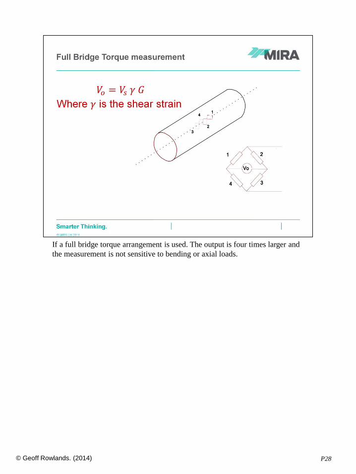
When a shaft is subjected to a torque or twisting force, the surface of the shaft

experiences shear strain. The amount of strain for a given torque is dependant

on the material properties and the radius of the shaft. A strain gauge can only

measure a linear change of length, and to measure the shear strain, the strain

gauge is placed at an angle of 45 degrees to the shaft axis. In order to calculate

the expected level of strain the given equation can be used.


If a full bridge torque arrangement is used. The output is four times larger and

the measurement is not sensitive to bending or axial loads.


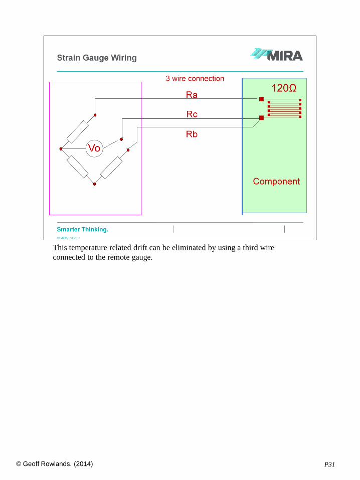
In this simple 2 wire configuration, the resistance of the connecting wires Ra

and Rb are in series with the gauge R2. The resistance of the wires will change

if there is a change in temperature. If the wires are long (>2m), this resistance

change may be significant and cause drifting errors on the signal, that seem to

be real strain.


This can be seen clearly in the equivalent circuit on the right.


This temperature related drift can be eliminated by using a third wire

connected to the remote gauge.


In this wiring configuration, the temperature drift is corrected. This is because

one wire appears in each arm of the right hand side of the bridge. If the

resistance of the wires Ra and Rb change by the same amount, the effect is

cancelled as adjacent arms subtract. Rc is the connection from the gauge to the

measuring instrument. Beacause the input impedance of the instrument is high,

no appreciable current flows through Rc, and so any change in resistance does

not cause a change in voltage seen by the instrument.


The output from the bridge when no strain is present should be zero volts. Due

to small inaccuracies in the strain gauges themselves, and also from the small

strains that result from the process of laying the gauge onto the test piece, there

is often an offset in the bridge voltage. It is important therefore to provide a

means of reducing this initial offset to zero. This is called bridge balancing or

“zeroing off”. There are several ways of achieving this, and one of which is

shown in the figure.

A high resistance potentiometer is placed across the supply apex points with its

wiper connected to one of the signal apex points. With the pot in its centre

position it adds no offset to the bridge but any deviation from the centre will

allow a resistance to be shunted across one arm of the bridge. The two

resistors R1 and R2 limit the amount of offset that can be provided, because

too much offset would lead to a non linear bridge output.

All strain gauge instrumentation amplifiers incorporate a

balancing facility but when using a general purpose amplifier or input card to a

PC based system this facility may be absent. A strain gauge bridge may be

brought into balance in these cases by soldering a suitable value of resistor

across one arm of the bridge, preferably near the gauge location.


One useful feature of strain gauges is that a calibration resistor can be placed

(shunted) across one arm of the bridge to simulate a known amount of strain.

This produces a step voltage change in the bridge output which provides a

check of the transducer /measurement system. The strain value simulated by

the resistor cannot change, and so gives a quick functional check of the whole

system. The choice of calibration resistor is important and should give a

reading that is similar to the expected signal. The calibration arrangement can

be simply that shown in the diagram where a particular value of resistor is

switched into parallel with one arm of the bridge. Depending on whether the

resistor is applied to the top arm or bottom arm, a positive or negative signal

can be simulated.


Strain Indicators.

The strain gauge may be connected directly into a strain

indicator box, a typical example is that made by Strainsense Ltd. Very

accurate strain readings can be made directly from this instrument which also

has facilities for balancing out any offset. This is a useful tool when the strain

gauges are first installed since it enables quick checking of gauge integrity and

will also show the magnitude of any offsets due to strain gauge laying faults.

It is also used when calibrating load cells that have been made using strain

gauges as the sensing element.


The strain gauge is a very common and versatile sensing element and will be

found in a great many types of transducer. This is useful since the same

instrumentation setup can therefore be used for a wide range of measurements.

In most cases the strain gauges will be in a full bridge arrangement. Each

transducer will have a calibration sheet which details the calibration

information needed to use the device.


Here are two examples of load cells. The one on the left is made from a “proof

ring” which is relatively compliant. This would be used for measuring small

forces accurately. The proof ring magnifies the strain appearing at the

locations where the strain gauges are placed. The example on the right is

much stiffer and can measure much larger loads. Both of these would be cased

in a steel housing to protect the gauges.


Strain gauge accelerometers have a mass that is suspended on a beam. When

the accelerometer is moved in the correct axis, the inertia of the mass acts

upon the beam and produces a bending load. This is then measured using the

bending arrangement we met before. The mass and sensing beam are all

mounted in a housing which is usually filled with a fluid to provide damping.

This is needed to prevent oscillation that happens in a spring/mass system. The

natural frequency of oscillations and the damping factor are two parameters

that dictate the maximum frequency of acceleration that can be measured.


In a pressure transducer, there are strain gauges mounted upon a diaphragm

sealed inside a housing with two chambers, One of these is connected to high

pressure and the other one may be connected to a lower pressure. The strain

reading will then be proportional to the pressure difference. If the pressure is

being compared to the normal ambient atmospheric pressure then the low

pressure port would be open. If an absolute pressure was needed then the low

pressure port would be sealed, and that side of the diaphragm would be at a

vacuum.


There are more examples that will be found of transducers that use strain

gauges and obviously there are other transducers that use other sensing

methods. The specification sheet for proprietary strain gauged transducers will

have common features, enabling the user to set up his data acquisition system

correctly. The information which is of interest is shown in the following list:

1. Bridge resistance. This will give the nominal

resistance of the strain gauges used, usually 120 or 350 ohms.

2. Excitation voltage. There is usually specified an

excitation voltage to be used with the transducer, 5 or 10 volts are common.

Obviously, the higher the excitation voltage, the more power is consumed by

the bridge. This can cause self heating effects, especially if the strain gauge is

mounted on a surface which has poor conductivity or low thermal mass.

3. Sensitivity. This is sometimes quoted as

millivolts per volt of excitation voltage per engineering unit. For instance

10mV/V

4. Calibration resistor. Sometimes a value of

calibration resistor is quoted together with its equivalent engineering value.

5. Colour coding of transducer connections.


41


42


These “pot”’s use a variable resistance as the sensing element. These are

simple and relatively cheap. The resistive material on the track of the pot is

trimmed to give very good linearity. They are available in many sizes and

types. One version has a spool of cable attached which winds out on a spring

return. This “string pot” is commonly used for larger displacements up to a

metre.


These string pots can be used for suspension measurements, control movement

measurements and other measurements where a linear pot would not be

suitable.


The LVDT is an alternative to the linear pot. In the past, the linear pot used a wire-wound

resistor track, and there were concerns that the wiper of the pot would eventually wear out the

track and cause errors. The LVDT uses inductive coupling and therefore has no contact

between the sensing parts.

There is a primary winding which is energised by an alternating voltage, and two secondary

windings placed one each side of the primary. An armature is fixed to a non magnetic rod

which is attached to the item to be measured. If the armature is closer to the right hand side

secondary as shown in the figure then there is better magnetic coupling between it and the

primary and the induced voltage will be higher than that induced in the left hand side. The two

secondary windings are connected in series opposition, that means that the voltage across the

output terminals is the difference between the two secondaries. It follows that when the

armature is central then the two secondaries are equal and opposite and the output is zero.

The output voltage is an AC voltage at the same frequency as the input

voltage but whose amplitude depends upon the position of the armature. The direction of the

displacement cannot be found by simply measuring the amplitude of the AC output because

there will be two positions either side of the centre zero position where the amplitude is the

same. The signal conditioning amplifier intended for use with this type of device includes a

phase sensitive detector (PSD). The PSD can discriminate the direction of the displacement.

Because the two secondaries are 180 degrees out of phase with each other, by comparing the

output waveform phase with the input waveform the direction of the movement can be found.


47


Piezoelectric sensors use a property of certain piezoelectric materials that

when a crystal of the material is subjected to a force, an electric charge is

generated across the outside faces. This charge although small can be

measured using a special Charge Amplifier. Electrical charge is measured in

Coulombs and as one coulomb is rather a lot of charge, these transducers have

an output in the order of pica-Coulombs pC or 10^-12 C. One Amp is defined

as 1 coulomb of charge flowing per second.

Since the crystal is connected to a measurement circuit, the charge will drain

away – much like discharging a capacitor. This means that if we apply a force

to the transducer we will see the measurement gradually reduce to zero. These

types of transducer are therefore only suitable for measuring varying forces not

steady ones. Piezoelectric accelerometers employ a similar principle, and have

the same limitation, in that they are only suited to measuring oscillations rather

than constant steady acceleration.


49


50


One of the most common devices for measurement of temperature is the

thermocouple. The thermocouple uses an effect called the Seebeck effect

which is that when two different metal wires are joined at their ends and one

end is at a higher temperature their is a small potential difference and a current

flowing. This can be amplified and gives a measurement. Over a useful range

of temperatures the output is acceptably linear. The sensing end of the

thermocouple is put into the place where the temperature is required. The other

junction is made inside the signal conditioning unit. The temperature of this

junction also needs to be measured since the potential difference depends on

the temperature difference between the two junctions. This can be measured by

a secondary transducer such as a thermistor within the unit. This is sometimes

known as a simulated ice reference because the temperatures are referenced to

zero degrees centigrade. It is also known as cold junction compensation.


RTD – Resistance temperature devices use the property that the resistance of

some materials varies with temperature.

The most commonly used is a Thermistor, which is a semiconductor device.

These can be made extremely small but require linearisation circuitry..

Platinum Resistance thermometers can be used in a bridge circuit like a strain

gauge. The resistance change is very linear with temperature.


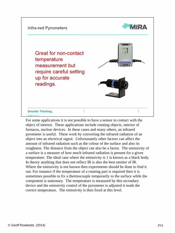
For some applications it is not possible to have a sensor in contact with the

object of interest. These applications include rotating objects, interior of

furnaces, nuclear devices. In these cases and many others, an infrared

pyrometer is useful. These work by converting the infrared radiation of an

object into an electrical signal. Unfortunately other factors can affect the

amount of infrared radiation such as the colour of the surface and also its

roughness. The distance from the object can also be a factor. The emissivity of

a surface is a measure of how much infrared radiation is present for a given

temperature. The ideal case where the emissivity is 1 is known as a black body.

In theory anything that does not reflect IR is also the best emitter of IR.

Where the emissivity is not known then experiments should be done to find it

out. For instance if the temperature of a rotating part is required then it is

sometimes possible to fix a thermocouple temporarily to the surface while the

component is stationary. The temperature is measured by this secondary

device and the emissivity control of the pyrometer is adjusted it reads the

correct temperature. The emissivity is then fixed at this level.


55


56


The WFT is measuring forces in the coordinates of the wheel which are

rotating. In order to resolve these into the vehicle coordinate system, a

measurement of wheel rotational angle is used. This requires a fixture to

restrain the outer part of the sensor so that rotation can be measured. If this

restraint is too “floppy”, it will flex when the vehicle hits a bump. This causes

an error in the rotational position which in turn causes errors in the wheel

forces. It is therefore very useful to record the rotational angle signal as it can

alert the user to any problems with restraint.


58


59


60


61


62


63


In this plot, the position of the vehicle was recorded as it was driven over a

road route. The analysis software was able to plot the route, and showed the

trace in a different colour for time spent in each gear ratio.

64


65


As has been described, all transducers are converting a physical quantity

which we want to measure into an electrical signal. It is vital to know that this

conversion is accurate or the recordings we make will be in error. This is why

calibration is so important. It gives us a connection between a known input

and the resulting voltage output. If the external conditions are the same, then

we can expect that the voltages we record will faithfully represent the wanted

measurement. It is however important to recognise that there are always errors

in any measurement. These may not be significant but we should know what

they are, and how to describe them.


Linearity is an expression of the closeness of the response of a system to a straight line. For

instance, if the response of the system can be modelled by an equation of the form y = mx+c ,

then it is said to have a linear response. A sensor need not have a straight line response and a

linearisation circuit may be used to make it linear. In these cases the linearity of the sensor

plus circuit would be useful to know. The linearity could be expressed as the maximum

deviation of any point from the straight line as a percentage of full scale. In this case 0.1 error

in a FS of 4 gives a linearity of 2.5%


Hysteresis is a term that describes how the measured value varies when

measurements are taken with an increasing input or a decreasing input. An

analogy in the mechanical engineering field is the backlash that occurs in

gears. It is best described using a diagram showing a hysteresis loop. This

effect is generally seen where there is something compliant in the

measurement system, like a rubber coupling.


Resolution is the smallest change in the measurement that can be detected by

the measurement system. An example would be the incremental resistance

change that could be seen on a wire wound potentiometer. Here the resolution

is the resistance of one turn. The other limiting factor for resolution is the

background noise in the system (more on noise later). On a digital voltmeter

the smallest resolution is dictated by the number of digits that can be

displayed. In a digital data acquisition system it may be the increment of the

measurement that is represented by the least significant bit of the analogue to

digital convertor.


Sensitivity gives a measure of the size of the output signal compared to the

input (supply) voltage.


What is noise?

There are many definitions that are possible but a comprehensive one is that noise is unwanted signal.

As an example, it may be required to measure the low frequency engine motions on its mountings, and an accelerometer could be mounted on the engine to do this task. The accelerometer also might pick up the much higher vibrations due to the engine firing pulses. In this case the higher frequency signal is noise. On another occasion the same set-up could be used to give engine speed using the higher frequency content. In this case the low frequencies would be considered to be noise.

A good analogy is that of tuning in a radio station. The airwaves are full of noise but in amongst it is the signal that you want. Your radio station is always someone elses noise however.

In a measurement environment there are usually sources of noise present and these can be identified with three different causes:

1. Inductive.

A changing magnetic field is produced by a nearby current carrier.

2. Capacitive.

Every conductor has some capacitance and can couple with an adjacent conductor that is carrying an alternating current,

3. Earth Loops.If there is an appreciable length between the transducer and the amplifier or power supply, connections at different points can form alternative loops for stray potentials causing interference. This type of interference is notoriously difficult to find since it does not remain stable but varies in a seemingly random way.


Inductive noise may be due to a power supply to some equipment outside the measuring system. the signal cables then become conductors in a changing magnetic field and have EMF's induced into them.

The cure is to use twisted pairs for signal cables. This has the effect that the emf's are induced firstly in one direction and then in the reverse direction. They therefore cancel out. Another guard against this is to use a differential amplifier. This only amplifies the difference between the signal high and signal low, if the noise is present on both, then it will be cancelled.

Capacitive noise is from a coupling with nearby metallic objects that can transmit noise. A remedy for this type of noise is to enclose the conductors in an earthed metal screen. Some signal cables are ready screened with a braided wire which affords a good level of protection but in very severe environments near to high power systems a specialised cable with solid continuous shielding may be required.

Earth Loops it is important that there is only one end of the system connected to ground. Connections at different points can form alternative loops for stray potentials causing interference. This type of interference is notoriously difficult to find since it does not remain stable but varies in a random way.

As a principle a decision must be made to earth each transducer at one end only. The most convenient is to earth the cables at the amplifier end of the system near to the power supply. The screens from the cables should only be connected at this end also. Some transducers have an earthed metal case and these may need to be mounted upon an insulated base.

The problem of earth loops can be eliminated on a vehicle installation by providing the amplifier and recorder with their own battery power supplies. This leaves the amplifier end of the system "floating" and means that some of the transducers can be allowed to connect to ground.


There are some classes of noise that do not seem to have

any useful data in them at all. These are random

fluctuations that occur due to small electrical effects. As

all Hi-Fi buffs will know, even a passive component like

a resistor can produce noise in an electrical circuit.

These sources of noise are always present and are broad

bandwidth in nature. They must be considered and

estimated because they limit the lower amplitude of

useful signal resolution.

At all times the main concern is to maximise the

wanted signal and minimise the noise and this is neatly

encapsulated in the concept of signal to noise ratio. (S/N

ratio).

This is usually expressed in decibels which is a

logarithmic relationship. In order to convert to decibels

the above equation can be used. As an example, 60 dB

signal to noise ratio means that the signal is 1000 times

larger than the noise.


76


77


78


79


80


81


Now we have chosen our transducers and have checked the calibration, its

time to connect them to the data recorder and actually collect some data.


83

© geoff rowlands. (2014) p1 - engineering integrity...

Documents