geography of poverty in mali - documents & reports - all documents | the world...
TRANSCRIPT

Report No. 88880-ML
Mali
Geography of Poverty in Mali
April 23, 2015
PREM 4
Africa Region
Document of the World Bank
Pub
lic D
iscl
osur
e A
utho
rized
Pub
lic D
iscl
osur
e A
utho
rized
Pub
lic D
iscl
osur
e A
utho
rized
Pub
lic D
iscl
osur
e A
utho
rized
i
CURRENCY EQUIVALENTS
(Exchange Rate as of March, 2015)
Currency unit = CFA franc (CFAF)
US$1.00 = CFAF 610
ABBREVIATIONS AND ACRONYMS
ACLED Armed Conflict Location and Event Dataset
AFD African Development Bank
AFISMA Afican-led International Support Mission to Mali
AICD Africa Infrastruture Country Diagnostic
AQIM Al-Qaeda in the Islamic Maghreb
CID Center for International Development
CPI Consumer Price Inflation
CSLP Cadre Stratégique de Lutte Contre la Pauvreté (Poverty Reduction
Strategy)
DNSI Discrimination and National Security Initiative
ELIM Enquête Intégrée auprès des Ménages
EMEP Enquête Malienne sur l’Evaluation de la Pauvreté
EMOP Enquête Modulaire et Permanente auprès des Ménages
F CFA Franc de la Communauté Financière Africaine
FEWSNET Famine Early Warning Systems Network
GDP Gross Domestic Product
GIS Geographic Information System
IDP Internal Development Program
IED Improvised Explosive Devises
IMF International Monetary Fund
INSTAT Institut National de la Statistique
MICS Multiple Indicator Cluster Survey
MICS Multiple Indicators Cluster Survey
MINUSMA United Nations Multidimensional Integrated Stabilization Mission in Mali
NOREF Norwegian Peacebuilding Resource Centre
PAPC Post-conflict Assistance Project
PIB Gross Domestic Product
RGPH Recensement Général de la Population et de l’Habitat
UEMOA West African States Monetary Union
UN United Nations
USD US dollar
WAEMU West African Economic and Monetary Union
WDI World Development Indicators
Regional Vice President:
Sector Director:
Country Director:
Sector Manager:
Task Team Leader:
Makhtar Diop
Ana Revenga
Paul Noumba Um
Pablo Fajnzylber
Johannes Hoogeveen
ii
Table of Contents
Aknowledgements .................................................................................................................... v
Executive Summary ................................................................................................................ vi
Introduction ........................................................................................................ 1
Mali by Agglomeration Type ............................................................................ 5
A. Introduction ......................................................................................................................................... 5 B. Classifying Mali by population density and size of the locality ......................................................... 6 C. Population Characteristics .................................................................................................................. 9 D. Spatial distribution of economic activities ........................................................................................ 14 E. Urban expansion and income growth................................................................................................ 19 F. Conclusion ........................................................................................................................................ 21
Mali by Livelihood Zone ................................................................................. 23
A. Introduction ....................................................................................................................................... 23 B. Livelihood zones in Mali .................................................................................................................. 23 C. Income and wealth ............................................................................................................................ 26 D. Patterns of consumption .................................................................................................................... 32 E. Access to services ............................................................................................................................. 34 F. Characteristics of poor households across livelihood zones ............................................................. 37 G. Discussion ......................................................................................................................................... 39
Explaining Well-being Using a Spatial Perspective ...................................... 42
A. Introduction ....................................................................................................................................... 42 B. Consumption ..................................................................................................................................... 42 C. New poverty lines for this report ...................................................................................................... 46 D. Poverty and poverty trends ............................................................................................................... 48 E. Caution When Interpreting poverty .................................................................................................. 59 F. Consumption and poverty and since 2010 ........................................................................................ 62 G. Ownership of assets .......................................................................................................................... 64 H. Other correlates of welfare ................................................................................................................ 65 I. Consumption regression.................................................................................................................... 69 J. Discussion ......................................................................................................................................... 73
Spatial Challenges to Service Delivery: Trading off Equity, Efficiency and
Quality 76
A. Introduction ....................................................................................................................................... 76 B. Unit costs and the delivery of services.............................................................................................. 76 C. Education: access versus quality ....................................................................................................... 78 D. Electricity .......................................................................................................................................... 89 E. Access to markets and roads ............................................................................................................. 91 F. Discussion ......................................................................................................................................... 97
Poverty Reduction and Growth in the Face of Spatial Challenges ........... 100
A. Introduction ..................................................................................................................................... 100 B. Poverty reduction requires accelerated growth ............................................................................... 100 C. Growth between 2000 and 2013 ..................................................................................................... 103 D. Spatially conscious strategies for accelerating growth ................................................................... 107
iii
Annex
Annex 1: Services trade policies for Member States of WAEMU ........................................................... 112
List of Tables
Table 2.1: City size and city rank (1987, 1998 and 2009) ............................................................................ 9 Table 2.2: Household characteristics by agglomeration type ..................................................................... 10 Table 2.3: Sorting of internal migrants (ages 15-64) by education level (2009) ........................................ 12 Table 2.4: Access to basic utilities (2009) .................................................................................................. 13 Table 2.5: Decomposition of the change in poverty between 2001 and 2010 ............................................ 20 Table 3.1: Wealth Characteristics According to Livelihood Zone ............................................................. 30 Table 3.2: Market access by livelihood zone .............................................................................................. 34 Table 3.3: Population density and access to basic utilities by livelihood zone (2009) ............................... 36 Table 4.1: Poverty incidence by livelihood zone ........................................................................................ 51 Table 4.2: Determinants of per capita consumption ................................................................................... 72 Table 5.1: Net enrollment in primary and secondary schools ..................................................................... 78 Table 5.2: Summary Data for Primary and Secondary Schools .................................................................. 86 Table 5.3: Percent of population living within a certain distance from a school ........................................ 88 Table 5.4: Road type and state of maintenance........................................................................................... 96 Table 7.1: Population estimates for census years...................................................................................... 102 Table 7.2: GDP per capita in 1987 prices ................................................................................................. 106 Table 7.3: Distance and time it takes to reach the main ports serving Mali ............................................. 107
List of Figures
Figure 1.1: Night-time lights 2012 ................................................................................................................ 1
Figure 1.2: Population density ...................................................................................................................... 2
Figure 1.3: Level of education of those aged 6 and above............................................................................ 4
Figure 2.1: Population urbaine et rurale au Mali .......................................................................................... 5
Figure 2.2: Voronoi polygons as approximation for the urban footprint of Bamako (2009) ........................ 6
Figure 2.3: Spatial distribution of urban areas (2009) ................................................................................. 7
Figure 2.4: Spatial distribution of the population (2009) .............................................................................. 8
Figure 2.5: Net interregional migration as percentage of population ......................................................... 11
Figure 2.6: Level of education of internal migrants as percentage of population ....................................... 11
Figure 2.7: Sectoral composition of employment by location (2009)......................................................... 14
Figure 2.8: Turnover of formal enterprises (2009-2010) and population (2009) ........................................ 15
Figure 2.9: Spatial distribution of jobs (1987, 1998 and 2009) .................................................................. 17
Figure 2.10: Contribution sectorielle par région et PIB par habitant (2009) .............................................. 18
Figure 2.11: GDP per capita and the degree of urbanization (1970-2012) ................................................. 20
Figure 2.12: Growth incidence curve for Bamako: 2001-2010 .................................................................. 21
Figure 2.13: Changes in economic sector of employment (*) .................................................................... 22
Figure 3.1: Livelihood Zones in Mali ......................................................................................................... 24
Figure 3.2: Household size by livelihood zone ........................................................................................... 25
Figure 3.3: Coping mechanisms for households affected by a crisis .......................................................... 27
Figure 3.4: Patterns of income generation by zone and household wealth ................................................. 29
Figure 3.5: Patterns of food consumption by zone and household wealth .................................................. 32
Figure 3.6: Quantities of milk and meat consumed by region (2001)......................................................... 33
Figure 3.7: Daily and weekly markets ........................................................................................................ 38
Figure 3.8: Percent of adult, non-pregnant women (15-49) that is anemic ................................................. 41
Figure 4.1: Distribution of rural and urban households by consumption quintile ...................................... 43

iv
Figure 4.2: Consommation par région: définitions différentes ................................................................... 44
Figure 4.3: Consumption per capita by livelihood zone ............................................................................. 45
Figure 4.4: Distribution of households by livelihood zone and by consumption quintile .......................... 46
Figure 4.5: Decomposition of the 2001 regional poverty lines in food and non-food components ............ 47
Figure 4.6: Decomposition of the newly estimated 2001 regional poverty lines ........................................ 47
Figure 4.7: Poverty trends: 2001-2010 by rural and urban ......................................................................... 48
Figure 4.8: Growth incidence curve national level: 2001-2010 .................................................................. 49
Figure 4.9: Poverty trends: 2001-2010, by region ...................................................................................... 51
Figure 4.10: Index of cereal production per capita (2000/1=100) .............................................................. 52
Figure 4.11: Production and value of production for cotton ....................................................................... 53
Figure 4.12: Index of per capita remittances from workers (2000=100) .................................................... 54
Figure 4.13: Road infrastructure in 1994 and 2007 .................................................................................... 55
Figure 4.14: Growth incidence curves by livelihood zone (2001-2010)..................................................... 55
Figure 4.15: Distribution of poor people across livelihood zones .............................................................. 59
Figure 4.16: Real consumption per capita between April-October in 2011 and 2013 ................................ 63
Figure 4.17: Projected poverty for 2013 calculated using EMOP consumption data ................................. 64
Figure 4.18: Ownership of televisions and motorbikes since 2001, by region ........................................... 65
Figure 4.19: Life expectancy and GDP per capita across Africa ................................................................ 66
Figure 4.20: Mortality rate and life expectancy by region .......................................................................... 67
Figure 4.21: Life expectancy (2009) and consumption per capita (‘000 FCFA) ........................................ 67
Figure 4.22: Malnutrition parmi des enfants 0-59 mois: 2006-2013 .......................................................... 67
Figure 4.23: Life expectancy and the degree of stunting (by region) ......................................................... 68
Figure 4.24: Malnutrition and poverty incidence ((by region) for children less than 5 years..................... 69
Figure 5.1: Population par densité .............................................................................................................. 77
Figure 5.2: Net enrollment in primary school 2011 and 2013 .................................................................... 79
Figure 5.3: Net primary school enrollment and fraction of population living within 2 km and 5 km from
primary school ............................................................................................................................................ 80
Figure 5.4: Map showing a 5km radius around every public schools ......................................................... 81
Figure 5.5: How school inputs would be reallocated for every region to be at the national average ......... 82
Figure 5.6 a & b: Distribution of newly constructed schools across regions (2009/10) and existing schools
(top panel) and people living within 2 km of a school (bottom panel) ....................................................... 83
Figure 5.7: Percent of children passing from one grade to the next in 2013 .............................................. 85
Figure 5.8: Number of households with access to electricity, by consumption quintile ............................. 89
Figure 5.9: Access to Roads ........................................................................................................................ 92
Figure 5.10: Percent of population living within 10 km of a market, by livelihood zone. ......................... 93
Figure 5.11: Minimum and maximum levels of quarterly per capita consumption, 2011. ......................... 94
Figure 5.12: Number of people per zone, living further than 10km from a market .................................... 95
Figure 5.13: Number of checkpoints per 100 km (1st quarter of 2013) ...................................................... 96
Figure 5.14: Location of savings banks ...................................................................................................... 99
Figure 6.1: Gini coefficients for selected countries in West Africa .......................................................... 101
Figure 6.2: GDP growth rates and growth rates needed to achieve various poverty targets by 2030 ....... 102
Figure 6.3: GDP per capita (columns) and its decomposition by sector ................................................... 104
Figure 6.4: Public and private investments as a percent of GDP .............................................................. 104
Figure 6.5: Cost to import a 20 foot container, 2005-2013 ....................................................................... 108
Figure 6.6: Internet Connectivity .............................................................................................................. 110
Figure 6.7: Map of Mineral Deposits ........................................................................................................ 111
List of Boxes
Box 6.1: An active industrial policy helps Ethiopia’s leather sector accelerate its growth ...................... 108
v
Aknowledgements
This study was prepared under the leadership of M. Sékouba Diarra Coordinator of the Cellule-
Technique of the CSLP, in collaboration with INSTAT and the World Bank. The INSTAT team
led by the Directeur Général, M. Seydou Moussa Traore, comprised Assa Doumbia-Gakou (Chef
de Département des Statistiques Démographiques et Sociales, M. Vinima Traore (Chef de
Division de la Cartographie), Abdoul Kdiawara (Chargé de Cartographie) and Siaka CISSE
(Chef de Division des Statistiques Démographiques et Sociales). The World Bank team led by
M. Johannes Hoogeveen (Senior Economist) comprised Yele Batana (Senior Economist), Brian
Blankespoor (GIS Specialist), Sebastien Dessus (Lead Economist), Cheikh Diop (Senior
Economist), Judite Fernandes (Team Assistant), Julia Lendorfer (Consultant), Yishen Liu
(consultant), Kristin Panier (Consultant), Mathieu Pellerin (Consultant), Harris Selod (Senior
Economist), Gael Raballand (Senior Economist) and Souleymane Traore (Team Assistant).
vi
Executive Summary
1. This study discusses the impact of economic geography and (low) population density
on development outcomes in Mali and explores how policies to reduce poverty could be
made more effective by taking these two factors into account.
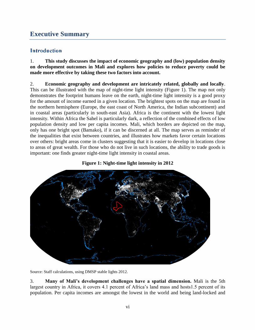
2. Economic geography and development are intricately related, globally and locally.
This can be illustrated with the map of night-time light intensity (Figure 1). The map not only
demonstrates the footprint humans leave on the earth, night-time light intensity is a good proxy
for the amount of income earned in a given location. The brightest spots on the map are found in
the northern hemisphere (Europe, the east coast of North America, the Indian subcontinent) and
in coastal areas (particularly in south-east Asia). Africa is the continent with the lowest light
intensity. Within Africa the Sahel is particularly dark, a reflection of the combined effects of low
population density and low per capita incomes. Mali, which borders are depicted on the map,
only has one bright spot (Bamako), if it can be discerned at all. The map serves as reminder of
the inequalities that exist between countries, and illustrates how markets favor certain locations
over others: bright areas come in clusters suggesting that it is easier to develop in locations close
to areas of great wealth. For those who do not live in such locations, the ability to trade goods is
important: one finds greater night-time light intensity in coastal areas.
Figure 1: Night-time light intensity in 2012
Source: Staff calculations, using DMSP stable lights 2012.
3. Many of Mali’s development challenges have a spatial dimension. Mali is the 5th
largest country in Africa, it covers 4.1 percent of Africa’s land mass and hosts1.5 percent of its
population. Per capita incomes are amongst the lowest in the world and being land-locked and
vii
located in a neighborhood of limited wealth, its opportunities for growth and development are
constrained. Mali cannot benefit from wealthy neighbors, population density is low and large
distances to West Africa’s coast limit opportunities for trade. Poverty is widespread and
significant spatial economic inequalities exist within the country. 40 percent of GDP is earned in
Bamako for instance. This economic dominance of the capital city spills over into welfare
outcomes: a person born in Bamako can expect to enjoy a level of per capita consumption that is
two and a half times higher than that of a person born in Ségou or Sikasso. The same person
from Bamako can also expect to live more than 6 years longer.
4. The crisis in north Mali which started in 2012 and continues to date has brought
questions of economic geography to the center of attention. The crisis raised questions about
whether it was fuelled by high levels of poverty and low levels of service delivery, whether too
many, or too few resources were spent in the north, whether it is reasonable to expect a
comparable level of service delivery in low density areas (the north) where unit costs are higher
and whether improved service delivery in the north could help secure peace.
5. To help answer such questions, and to analyze how to reduce poverty in Mali as a
whole, this study uses different sources of information to analyze the diversity of livelihood
patterns, in access to services and in living standards. The study uses quantitative information
from household surveys, population and firm censuses, administrative and geographic data and
qualitative information about livelihoods. By combining data from different sources we are able
to shed new light on various development issues: how different sources of income are associated
to poverty reduction, why poverty in Sikasso remains stubbornly high (though it may be lower
than previously thought) as well as the relationship between improved access to markets, poverty
and vulnerability. We discuss how differences in service delivery are associated with population
density and show the primacy of Bamako in the formal economy of the country. In the final
section we explore what it would take to reduce poverty by half by 2030.
6. The 2009 World Development Report (WDR) on Economic Geography offers useful
guidance to policy makers grappling with issues of economic geography. The WDR argues
that to reduce poverty, economies need to integrate economically. To this end, policy makers
have three instruments at their disposal: spatially-blind institutions (i.e. services that are offered
to all, irrespective of where one lives); connectivity (such as roads and railways), and spatially
targeted interventions (such as special incentives for enterprises, public works, agriculture
extension schemes, training programs). This study argues that the authorities will need to employ
all three policy instruments, while emphasizing that if the objective is poverty reduction, most
attention should be focused on spatially blind approaches.
7. A number of new analyses have been prepared to inform this study. A
reclassification of Mali’s rural and urban areas based on population density allows us to re-
estimate the degree of urbanization; a re-estimation of the poverty line addresses problems with
food-shares in the existing poverty lines, while a comparison between asset based and
consumption based poverty measures raises questions about the accuracy of the (consumption
based) poverty estimates for Sikasso. Integration of census and household surveys with
information on livelihoods permits us to link information about changes in poverty to sources of
income and growth –something that was not possible before. The study is informed by new

viii
estimates of market access (using population density and infrastructure) and of the size of
informal cross-border trade between Mali and Algeria. Finally, poverty- growth projections shed
light on the question whether significant reduction in poverty can be achieved by 2030.
8. Using a measure of population density to define rural and urban areas, we find that
Mali’s economy is predominantly rural: 73 percent of the population resides in rural areas. We
identify 75 towns and cities hosting 3.9 million people—out of a population of 14.5 million.
Bamako is the dominant city. It hosts more than 2.1 million people (15 percent of the
population), five times more than the next three largest cities combined: in Ségou, Sikasso and
Kayes live 166,000, 143,000 and 127,000 people respectively (3 percent of the population).
9. Agriculture remains important, in rural areas but also in cities. In rural areas 86
percent of all jobs are in agriculture as opposed to 3 percent in Bamako. Agricultural jobs
represent a significant portion of employment; in small cities with less than 30,000 people, 43
percent of people work in agriculture; in cities with over 30,000 inhabitants this is 24 percent (it
is 3 percent in Bamako). Inversely, the shares of administrative jobs, of service jobs and, above
all, of trade activities increase with city size. In the four largest cities, trade jobs account for 28
to 32 percent of employment.
10. The location of formal activities is skewed towards Bamako. Irrespective of whether
one considers the number of formal enterprises, or their turnover, Bamako is the dominant
location. The primacy of Bamako in generating income is such that with 15 percent of the
population about 40 percent of GDP is generated. With 18 percent of GDP, the region of Kayes
is another important contributor to GDP followed by Sikasso (12 percent) and Koulikoro (11
percent).
11. In the face of rapid population growth, Mali is urbanizing. The population of
Bamako grew at 3.7 percent on average per year between 1987 and 1998; between 1998 and
2009 growth accelerated to an annual average of 6.1 percent. At this rate of growth, the
population of Bamako will exceed 4 million by 2020.1 By contrast, between 1998 and 2009,
secondary cities and rural locations grew at 3.6 percent and 2.3 percent respectively. Because
cities grow at a faster pace than rural areas the country is urbanizing. In this context it is
worthwhile to note the rapid, and increasing, rate of general population growth: the population
growth rate accelerated from about 1.6-1.7 percent between 1976 and 1987, to 3.1-3.6 percent
between 1998 and 2009. Such a rapid rate of population growth has consequences for jobs,
unemployment and the demand for social services. It increases pressure on cultivable (irrigated)
land and access to water and has the potential to become a driver of social change and possibly
even conflict in the future.
12. While Bamako’s population increased rapidly, agglomeration effects are not leading
to a process of economic growth and transformation. Between 2001 and 2010 per capita
1 The crisis in Côte d’Ivoire may have contributed to the acceleration of Bamako’s growth, as migrants who used to
travel south, opted to go to Bamako instead. If this is the case, the growth of Bamako can be expected to slow down
as the economy of Côte d’Ivoire picks up.

ix
income growth hovered around 1 percent per annum for most households, except for the top 10
percent who became less well off. Decomposing the overall change into two periods, 2001-2006
and 2006-2010, we find that the city transformed from a place with high levels of per capita
growth in the early 2000s to a place in which per capita consumption growth is negative. This
lack of dynamism is corroborated by other evidence: a comparison of the 2009 and 1998
population censuses shows that the sectoral composition of jobs has changed little; macro-
economic statistics show that the secondary sector (which is largely located in Bamako) did not
grow – at least not in per capita terms.
13. Higher levels of consumption in Bamako are largely explained by higher levels of
education. Levels of consumption in Bamako are on average twice as high as elsewhere in the
country. This can be attributed to levels of education being much higher in Bamako. Bamako
also attracts the most qualified migrants (79 percent of internal migrants with a tertiary education
end up in Bamako; by contrast only 55 percent of migrants with no education go to Bamako).
14. Livelihoods in Mali vary from nomadic trade and pastoralism, to sedentary farming
and fishing to living as city dweller and come with a clear spatial demarcation. Rainfall is a
decisive factor in identifying different rural livelihood areas as rainfall drives the degree of
dependence on livestock herding in certain areas, the use of arable land in others and the degree
of dependence on labor and other sources of income. Following the rainfall pattern, four broad
livelihood areas are identified: (i) the dry area of the north, (ii) a transitional area stretching from
Kayes in the west to the border with Niger in the east, (iii) the agricultural area of the south and
(iv) various smaller areas defined by the potential to irrigate using water from the Niger river.
Each of these areas can be further
subdivided into a total of 12 rural
livelihood zones and one urban
livelihood zone (Bamako).
In the dry area nomadism,
transhumant pastoralism and
long distance trade are
dominant. Kidal, Gao and
Tombouctou lie in this area.
Households living in this area
have strong commercial and
social ties with Algeria, but
also with Niger, Burkina Faso
and Mauritania (livelihood
zones 1 & 2 in Figure 2).
In the transitional area
households rely on a mix of
income derived from
transhumant livestock
rearing, remittances from
migration and agriculture as
Figure 2: Livelihood zones identified for Mali
Source: FEWSNET 2010.
x
rainfall is too low to make a living based on crop income alone. The further south one goes
in this area, the less the dependence on livestock and the greater the importance of
cultivation. The location of this transitional zone means that it dominates the north-south
commercial axis with grain moving from the south towards the food deficit dry area in the
north, and with livestock and seasonal migrants moving from the north towards the south
(livelihood zones 4, 5, 8 & 9 in Figure 2).
The agricultural area in the south where farming is most productive. Income from livestock
is no longer important in this area as rainfall is adequate for households to fully depend on
income from cultivation. The main crops grown are cereals (sorghum, millet and maize),
cotton as well as fruits. It is the area with the highest population density but also the area
with the largest number of poor people (livelihood zones 10, 11 & 12 in Figure 2).
The potential to irrigate defines the last livelihood area. This area includes the fluvial basin
of the Niger stretching from Tombouctou to the international border between Mali and Niger,
it includes the delta stretching from Tombouctou to south of Mopti as well as the Office du
Niger, a manmade irrigation scheme reclaimed from the Sahel by irrigation canals and dams
(livelihood zones 3, 6 & 7 in Figure 2).
15. Livelihood areas not only characterize the ways household earn a living, they are
associated with other factors such as population density and household size. Population
density increases with the productivity of the land and varies from less than 2 inhabitants / km2
in the dry and inhospitable livelihood area of the north, to 18 in the transitional area to over 52
inhabitants / km2 in southern Mali. Livelihood zones with irrigation potential have higher levels
of population density than their surrounding areas: 27 inhabitants / km2 in zone 3 along the
borders of the river Niger as opposed to 1.9 in zone 2 through which the river flows; 33
inhabitants / km2 in zone 6, the Niger delta as opposed to 7.7 in zone 4 in which the delta lies;
181 inhabitants / km2 in the Office du Niger as opposed to 28 in the surrounding livelihood
zones. Family size is also correlated with the different types of livelihood. The largest families
(around 11 household members) are found in the southern agricultural area and smaller families
(average household size of 7 to 8) in zones where fisheries and commerce are dominant (the dry
area and zones with irrigation potential). The presence of large families in livelihood zones
where agriculture is dominant is explained by the fact that labor markets function poorly (a
characteristic common to all land-abundant tropical, rain-fed agriculture), which in combination
with very high demands for labor during the short planting season, creates a preference for
family labor.

xi
16. Access to markets, seasonal variations in consumption and differences in
malnutrition are associated with different livelihood zones. Access to markets (calculated as
the number of consumers that can be reached within a given time frame) is best around the urban
centers of south Mali (Figure 3), it is relatively good in the high agricultural potential areas of the
south and poor in all other areas. The livelihood area with (irrigated) agricultural potential in the
north such as the fluvial basin of the Niger (zone 3) and the Niger delta (zone 6) are
characterized by limited market
access. Differences in market
access are, in turn, associated
with differences in
consumption vulnerability,
which is the combined effect of
low average levels of
consumption and seasonal
differences in consumption
(possibly because the poorest
who depend on food purchases
pay higher prices in isolated
areas). Of particular concern is
the variation that occurs in the
northern livelihood zones in
which households practice
agriculture (zones 3, 4, 5 and 6)
but not in the desert (zones 1
and 2) where –at least prior to
the security crisis, levels of
household consumption were
relatively elevated and its
seasonal variation limited. The
northern agricultural zones are
also the zones where levels of
acute malnutrition (wasting)
are highest. By contrast, levels
of chronic malnutrition (stunting) are particularly high in the southern parts of the country, where
households rely almost exclusively on income from farming and where little animal protein is
consumed.
17. Between 2001 and 2010 poverty as well as inequality decreased rapidly. Poverty
incidence declined from 51 percent to 41 percent; the Gini coefficient dropped from 0.40 to
0.33. Despite the decline in poverty incidence the number of poor increased by around 360,000
as a consequence of Mali’s high population growth. The number of non-poor increased by
approximately 3 million.
18. The evolution of poverty since 2010 is not clear. In 2001, 2006 and 2010
EMEP/ELIM surveys collected comparable consumption information from which poverty
Figure 3: Access to Markets.
Source: RGPH 2009. Authors’ calculations.

xii
estimates could be derived. In 2011 and 2013 EMOP surveys were fielded which collect
consumption information differently. Consequently poverty estimates before and after 2010
should not be compared. A comparison of information from EMOP 2011 and 2013 suggests that
in south Mali (the north was not covered by EMOP 2013) per capita consumption declined by 10
percentage points. Macro data and predictions from a general equilibrium model of the economy
contradict this and suggest consumption declined by 2 percent per capita. Depending on which
estimates are used to predict poverty starting from the latest comparable survey, one finds that all
gains in poverty reduction were wiped out (poverty incidence returned to 51 percent) or that
there was hardly any change since 2010. The EMOP data for 2013 are preliminary and it is
critical that a final dataset becomes available. It is even more important that a survey is fielded
that collects consumption information that is comparable to what was collected by EMEP/ELIM.
19. Information on the ownership of consumer durables is comparable across surveys. Ownership increased significantly between 2001 (EMEP) and 2011 (EMOP) and stagnated
thereafter. Since 2001 the fraction of households owning fridges doubled from 5 percent to 11
percent, while the ownership of televisions almost tripled going from 14 percent to 37 percent.
The increase of mobile phone ownership amongst households is remarkable. It increased from
virtually zero in 2001 to 67 percent in 2011. A similar trend is observed with respect to motor
bikes. Over the course of
one decade ownership
more than tripled from 17
percent to 48 percent. The
increase in asset
ownership among
households can be
attributed to the drop in
real prices for many
consumer durables and the
increase in disposable
income amongst the
poorest households. Post
2011 asset ownership
declined slightly.
20. To better
understand the drivers
of change in poverty, we
focus our analysis on the
2001-2010 period for
which three comparable
household surveys are
available. Over this
period per capita consumption increased 2.2 percent, from FCFA 142,000 to FCFA 145,000.
That this tiny increase in consumption is associated with a 10 percentage point decline in poverty
is explained by the fact that for the poorest consumption grew most rapidly, while for better off
households consumption grew slowly or even declined (for households in the top wealth quintile
Figure 4: Growth incidence curve national level: 2001-2010(*)
(*) The band around the line represents the 95% confidence interval
Source: EMEP 2001, ELIM 2006 and ELIM 2010. Authors’ calculations

xiii
consumption fell – see Figure 4). These results have to be interpreted with care because the large
dependence on rain fed agriculture implies that weather differences are likely to have more
consequences for (short-term) welfare than policy changes. Moreover difficulties with the way in
which consumption quantities are ‘priced’ (using local prices, implying low monetary levels of
consumption in the grain baskets of the country) call for caution in the interpretation of
consumption and poverty data, including the data presented on the 2009 poverty map.
21. Most of the decline in poverty was realized between 2001 and 2006, while between
2006 and 2010 little changed. This is illustrated by the growth incidence curves at the bottom of
Figure 4. It shows how between 2001 and 2006 per capita incomes increased for all wealth
groups. This changed in the period between 2006 and 2010. Now only the poorest households
experienced positive consumption growth. The middle class experience no growth and per capita
consumption for those in the top 30 percentiles declined.
Table 1: Poverty incidence, population and population density by livelihood zone
Zone Description 2001 2006 2010 Population Density
1 Nomadism and trans-Saharan trade 12.7 42.3 37.5 69,762 0.2
Standard error 3.4 10.4 5.0
2 Nomadic and transhumant pastoralism 20.6 17.1 22.3 593,743 1.9
Standard error 7.9 4.6 2.3
3 Fluvial rice and transhumant livestock rearing
(agropastoral)
46.0 37.8 29.7 165,566 27.3
Standard error 8.9 9.6 3.7
4 Millet and transhumant livestock rearing 68.2 42.5 58.2 1,043,451 7.7
Standard error 4.7 4.2 4.3
5 Dogon plateau -- millet, shallots, wild foods and
tourism
82.4 87.5 40.7 264,780 44.5
Standard error 4.0 9.9 9.2
6 Niger delta - rice and livestock rearing
(agropastoral)
23.7 19.5 29.6 881,758 33.0
Standard error 4.9 5.3 2.9
7 Office du Niger (irrigated rice) 40.8 57.0 21.2 351,805 180.9
Standard error 8.3 9.2 6.3
8 North-west remittances, sorghum and transhumant
livestock rearing
62.6 30.4 19.6 791,037 18.4
Standard error 4.4 3.7 3.8
9 West and central rain-fed millet/sorghum 49.9 45.7 42.5 3,357,547 27.7
Standard error I 2.6 2.9
10 Sorghum, millet and cotton 54.6 70.9 74.3 1,291,649 52.3
Standard error 6.7 5.4 3.9
11 South maize, cotton and fruits 71.8 56.2 52.0 3,393,992 33.7
Standard error 3.0 2.8 3.1
12 South-west maize, sorghum and fruits 80.1 63.0 52.7 510,350 19.2
Standard error 5.6 6.4 6.0
13 Bamako 14.1 6.3 7.6 1,810,366 7,380.0
Standard error 3.4 2.3 1.1
Mali 50.9 41.7 41.1
Standard error 1.7 1.5 1.3 14,525,806 11.6
Source: ELIM 2001, 2006 and 2010. RHPH 2009. Authors’ calculations.
22. Internal (permanent) migration was not a driver of poverty reduction. Decomposing
the change in poverty that occurred between 2001 and 2010 (a decline by 9.9 percentage points)
we find that most of this change (9.4 percent) was due to a reduction in poverty amongst people
xiv
Figure 5: Cereal production per capita
(annual averages)
Source: Ministry of Agriculture 2014
75.4
55.2
75.1
27.9
106.3
84.7
138.1
101.9
0.0
20.0
40.0
60.0
80.0
100.0
120.0
140.0
160.0
Millet Sorghum Rice Maize
Cer
eal
pro
du
ctio
n
(k
g p
er c
ap
ita
)
2000-2003 2010-2013
who continued to reside in their location of origin (mostly in rural areas). The contribution to
poverty reduction of people shifting from rural to urban areas is tiny (0.3 percent) suggesting that
most of the migrants who move to urban areas were non-poor in their location of origin.
23. Even though the household surveys were not designed to be representative by
livelihood zone it is possible to estimate poverty by zone. We present these estimates in table 1
but urge the reader to take into account the standard errors when interpreting the results as in
some instances they are larger than usual.
24. As rule of thumb poverty is highest in southern zones where households rely on rain
fed agriculture (zones 4, 5, 9, 10, 11 and 12) and lower in the north of the country.
Households depending on nomadic and transhumant pastoralism living in zone 2, those
depending on irrigated agriculture (zones 3, 6 and 7) and those in north west Kayes who combine
income from remittances with livestock rearing (zone 8) are comparatively better off: their levels
of poverty are below 30 percent. With a rate of poverty of 74.3 percent the incidence of poverty
is highest in the area south of Ségou where sorghum, millet and cotton are grown (zone 10). The
incidence of poverty is lowest in Bamako (7.6 percent) and in zone 8 in north-west Kayes (19.6
percent).
25. In south Mali’s most populous areas (zones 9, 10, 11 and 12) divergent poverty
trends are observed. In zone 10, the area south of Ségou, poverty increased from 55 percent in
2001 to 74 percent in 2010. By contrast in west and central Mali (zone 9: millet and sorghum)
and in the two most southern zones (zones 11 and 12 where maize, cotton, fruits and sorghum
are grown) poverty decreased. Particularly in the latter two zones did poverty decline
significantly from 72 percent in 2001 to 52 percent in 2010. The divergent patterns of poverty
reduction within the region of Sikasso (zones 10, 11 and 12 lie in Sikasso region) challenge the
view that poverty in Sikasso is stagnant. Whereas this is holds for the regional as a whole, at sub-
regional (zonal) level considerable dynamism.
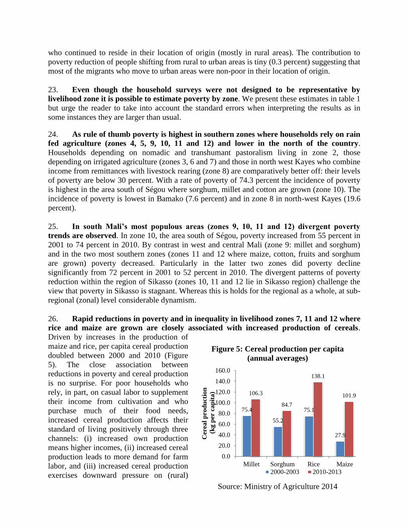
26. Rapid reductions in poverty and in inequality in livelihood zones 7, 11 and 12 where
rice and maize are grown are closely associated with increased production of cereals.
Driven by increases in the production of
maize and rice, per capita cereal production
doubled between 2000 and 2010 (Figure
5). The close association between
reductions in poverty and cereal production
is no surprise. For poor households who
rely, in part, on casual labor to supplement
their income from cultivation and who
purchase much of their food needs,
increased cereal production affects their
standard of living positively through three
channels: (i) increased own production
means higher incomes, (ii) increased cereal
production leads to more demand for farm
labor, and (iii) increased cereal production
exercises downward pressure on (rural)
xv
food prices. It is noteworthy that poverty amongst households living in the Niger delta (zone 6)
has increased, suggesting that they have not been able to benefit from increased rice production –
the reason why deserves to be explored.
27. For households in livelihood zone 8 whose incomes come from remittances, sorghum
cultivation and transhumant livestock rearing, the rapid decline in poverty is the combined
effect of increases sorghum production (Figure 5) and a three-fold increase in per capita
remittances. We find no association between (the value of) cotton production and poverty
reduction. This may be because ever since financial and management problems started to plague
the CMDT, cotton is primarily grown by non-poor households while poor households switched
to cereals. Consequently increased cotton production only benefits poor households indirectly
through the labor market and through improved market accessibility and the increased
availability of inputs brought about by the CMDT.
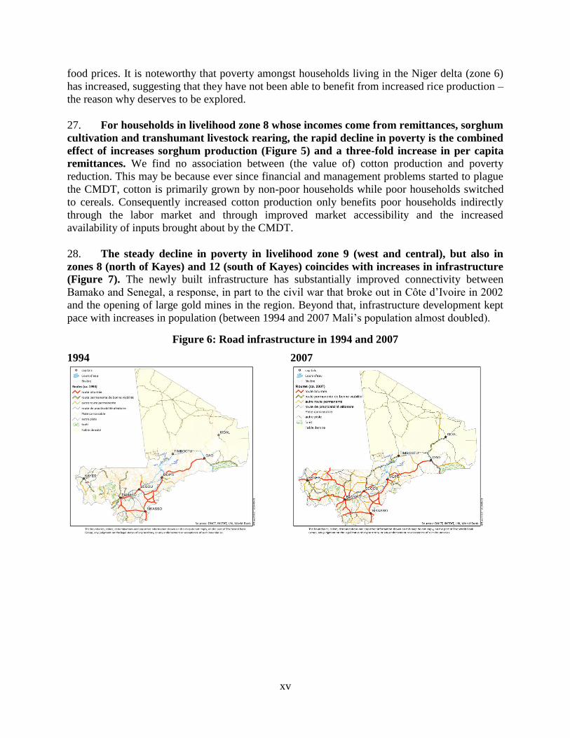
28. The steady decline in poverty in livelihood zone 9 (west and central), but also in
zones 8 (north of Kayes) and 12 (south of Kayes) coincides with increases in infrastructure
(Figure 7). The newly built infrastructure has substantially improved connectivity between
Bamako and Senegal, a response, in part to the civil war that broke out in Côte d’Ivoire in 2002
and the opening of large gold mines in the region. Beyond that, infrastructure development kept
pace with increases in population (between 1994 and 2007 Mali’s population almost doubled).
Figure 6: Road infrastructure in 1994 and 2007
1994 2007
xvi
Source: ELIM 2010. Authors’ calculations.
0.2 1.6
0.9
9.9 2.2
5.0 1.5
2.4
24.2
14.9
30.4
4.7 2.3
1. Nomadism and trans-Saharan trade
2. Nomadic and transhumant pastoralism
3. Fluvial rice and transhumant livestock rearing
4. Millet and transhumant livestock rearing
5. Dogon plateau -- millet, shallots, wild foods,
tourism6. Niger delta - rice and livestock rearing
7. Office du Niger (irrigated rice)
8. Remittances, sorghum, transhumant livestock
rearing9. West and central rainfed millet/sorghum
10. Sorghum, millet and cotton
11. South maize, cotton and fruits
12. South-west maize, sorghum and fruits
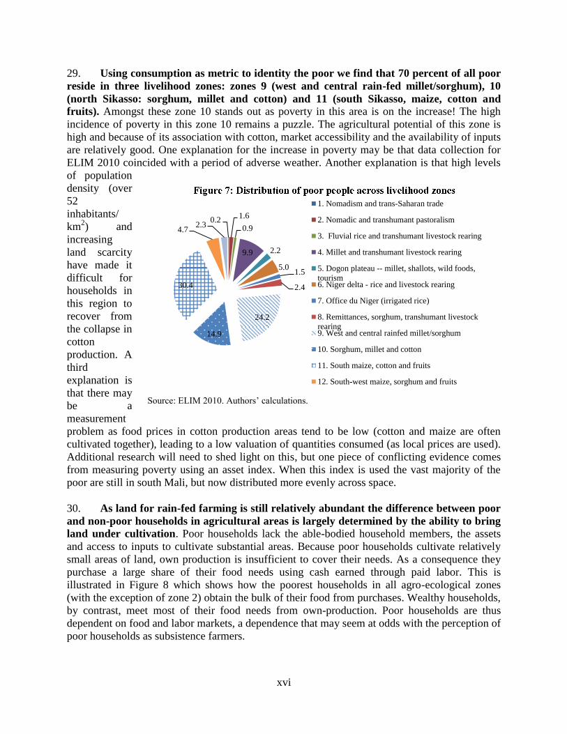
29. Using consumption as metric to identity the poor we find that 70 percent of all poor
reside in three livelihood zones: zones 9 (west and central rain-fed millet/sorghum), 10
(north Sikasso: sorghum, millet and cotton) and 11 (south Sikasso, maize, cotton and
fruits). Amongst these zone 10 stands out as poverty in this area is on the increase! The high
incidence of poverty in this zone 10 remains a puzzle. The agricultural potential of this zone is
high and because of its association with cotton, market accessibility and the availability of inputs
are relatively good. One explanation for the increase in poverty may be that data collection for
ELIM 2010 coincided with a period of adverse weather. Another explanation is that high levels
of population
density (over
52
inhabitants/
km2) and
increasing
land scarcity
have made it
difficult for
households in
this region to
recover from
the collapse in
cotton
production. A
third
explanation is
that there may
be a
measurement
problem as food prices in cotton production areas tend to be low (cotton and maize are often
cultivated together), leading to a low valuation of quantities consumed (as local prices are used).
Additional research will need to shed light on this, but one piece of conflicting evidence comes
from measuring poverty using an asset index. When this index is used the vast majority of the
poor are still in south Mali, but now distributed more evenly across space.
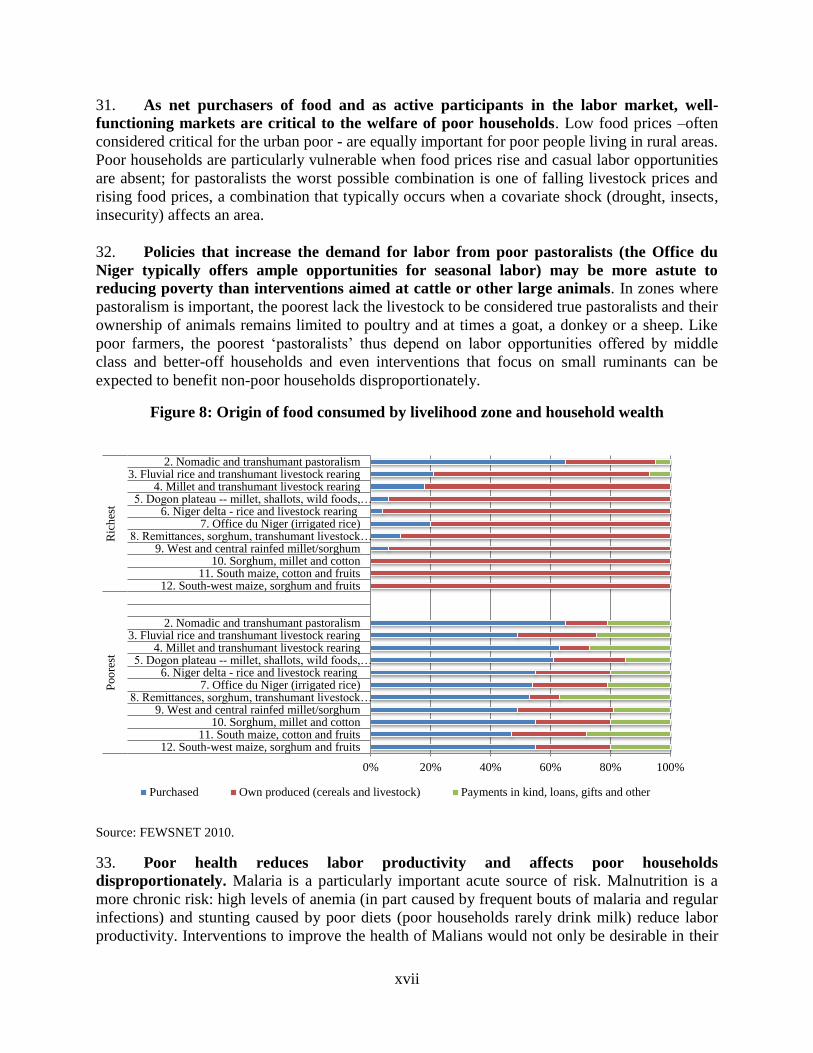
30. As land for rain-fed farming is still relatively abundant the difference between poor
and non-poor households in agricultural areas is largely determined by the ability to bring
land under cultivation. Poor households lack the able-bodied household members, the assets
and access to inputs to cultivate substantial areas. Because poor households cultivate relatively
small areas of land, own production is insufficient to cover their needs. As a consequence they
purchase a large share of their food needs using cash earned through paid labor. This is
illustrated in Figure 8 which shows how the poorest households in all agro-ecological zones
(with the exception of zone 2) obtain the bulk of their food from purchases. Wealthy households,
by contrast, meet most of their food needs from own-production. Poor households are thus
dependent on food and labor markets, a dependence that may seem at odds with the perception of
poor households as subsistence farmers.
xvii
31. As net purchasers of food and as active participants in the labor market, well-
functioning markets are critical to the welfare of poor households. Low food prices –often
considered critical for the urban poor - are equally important for poor people living in rural areas.
Poor households are particularly vulnerable when food prices rise and casual labor opportunities
are absent; for pastoralists the worst possible combination is one of falling livestock prices and
rising food prices, a combination that typically occurs when a covariate shock (drought, insects,
insecurity) affects an area.
32. Policies that increase the demand for labor from poor pastoralists (the Office du
Niger typically offers ample opportunities for seasonal labor) may be more astute to
reducing poverty than interventions aimed at cattle or other large animals. In zones where
pastoralism is important, the poorest lack the livestock to be considered true pastoralists and their
ownership of animals remains limited to poultry and at times a goat, a donkey or a sheep. Like
poor farmers, the poorest ‘pastoralists’ thus depend on labor opportunities offered by middle
class and better-off households and even interventions that focus on small ruminants can be
expected to benefit non-poor households disproportionately.
Figure 8: Origin of food consumed by livelihood zone and household wealth
Source: FEWSNET 2010.
33. Poor health reduces labor productivity and affects poor households
disproportionately. Malaria is a particularly important acute source of risk. Malnutrition is a
more chronic risk: high levels of anemia (in part caused by frequent bouts of malaria and regular
infections) and stunting caused by poor diets (poor households rarely drink milk) reduce labor
productivity. Interventions to improve the health of Malians would not only be desirable in their
0% 20% 40% 60% 80% 100%
12. South-west maize, sorghum and fruits11. South maize, cotton and fruits
10. Sorghum, millet and cotton9. West and central rainfed millet/sorghum
8. Remittances, sorghum, transhumant livestock…7. Office du Niger (irrigated rice)
6. Niger delta - rice and livestock rearing5. Dogon plateau -- millet, shallots, wild foods,…
4. Millet and transhumant livestock rearing3. Fluvial rice and transhumant livestock rearing
2. Nomadic and transhumant pastoralism
Poo
rest
Ric
hes
t
Purchased Own produced (cereals and livestock) Payments in kind, loans, gifts and other

xviii
own right, it would have an immediate economic benefit as it would improve labor productivity.
Moreover it would be a pro-poor policy measure. Not only is the capacity to work is the main
(and often only) asset of poor households, with fewer able bodied household members, poor
households are particularly vulnerable to the negative welfare consequences of a health shock.
34. The poorest often lack the means to migrate to casual labor opportunities, either
because they have too few able-bodied household members or lack the cash to pay for
transport. Many households engage in temporary labor migration as it offers an important
source of cash, more so to households in the north where livelihoods are more uncertain and
opportunities for work more restricted. Very poor households, however, lack the means to move
to where demand for labor is highest and depend on casual labor opportunities nearby.
35. Low population density creates trade-offs between equity (access to public services
for all) and efficiency (providing service access to as many people as possible for a given
budget). The unit cost of service provision is largely determined by fixed costs in relation to the
number of people that use a service. Services requiring large investments such as piped water or
electricity can only be offered in a cost-effective manner in areas where population density is
high: cities. To offer a comparable service in a low density area, a service would have to require
lower fixed costs. This explains why tarmacked roads are found in cities, and dirt tracks in low
density areas like rural villages. It also explains why the provision of the same level of service in
north Mali (where population density is low) will cost more than elsewhere in the country.
36. Low levels of income, a small public resource envelope, low population density and a
large unmet demand for public services, make the question how to make public services
cost-effective, pressing. How pressing this problem is can be illustrated with an example for
secondary schools. Imagine that the maximum distance a secondary student can be expected to
travel is 7 km (one way). The catchment area of a school is then 154 km2 (πr
2). Next assume that
a secondary school requires at least 250 students to operate in a cost-efficient manner. We know
that 30 out of every 100 children complete primary school and are eligible to go to secondary
school (Figure 11) and that children of secondary school age (those aged 13-18) make up 14
percent of the population. We can now calculate that to run a secondary school efficiently,
population density needs to be about 39 people per square kilometer. Only 50 percent of the
population of Mali lives in such areas. Does this mean that half the population should be
deprived of the opportunity access to a secondary school? This example illustrates not only how
efficiency is a prerequisite to achieve equity (spatially blind service delivery), it also shows that
efficiency and equity are related to aspects of quality (if the primary school retention rate were
higher, the density requirement for secondary schools would go down). The example also makes
clear that the challenges of service delivery in low population density areas extend beyond north
Mali. Only 12 of the 50 percent who live in areas with too low a density to offer secondary
education stay in the north. The remainder lives elsewhere.
37. To explore how to make public services available to all three case studies are
presented. They have been selected because they require different levels of fixed costs
(relatively low in the case of primary education; high in the case of electricity) and because of

xix
their relevance for economic integration (access to markets). Based on these case studies some
policy implications are presented at the end of the section.
Primary education
38. Levels of education in Mali are very low. Almost sixty percent of the population aged
six and above has no education at all, approximately 35 percent has primary education and less
than eight percent has secondary education or higher. In the northern regions of the country,
Mopti, Tombouctou and Kidal more than 80 percent of the population has not gone to school at
all. In Bamako the situation is better but even here as many as 34 percent of the population never
went to school. With an average of 2.38 years of education, Malians aged 15 and above are the
third least educated in the world.2 Only Mozambique and Niger do worse.
39. Despite improvements, school enrollment remains low. According to the EMEP/ELIM
surveys net primary school enrollment increased from 31 percent in 2001 to 54 percent by 2010.
Enrollment varies across the country from as low as 35 percent in Tombouctou and Mopti to 83
percent in Bamako (Figure 9). The poorest households who had the lowest enrollment rate in
2001 benefited most (in relative terms), but failed to close the gap in enrollment with the richest
households. In 2010, the net enrollment rate for children from the poorest households was 46
percent; for children from the wealthiest households it was 71 percent. Enrollment in secondary
schools went up from 10 percent in 2001 to 28 percent by 2010.
Figure 9: Net primary school enrollment and fraction of population living
within 2km and 5km from primary school
Source: EMOP 2011 (enrollment) and RGPH 2009 (distance). Authors’ calculations.
40. In terms of school construction much has been achieved: more than 80 percent of
the population lives within 2 km of a school. Comparisons of the fraction of the population
that live within 2 km from a school with enrollment rates, suggest that access is not the
2 Data downloaded from www.barrolee.com (June 2014). Barro, Robert and Jong-Wha Lee, April 2010, "A New
Data Set of Educational Attainment in the World, 1950-2010." Journal of Development Economics, 104(184-198).
63 64 66 59
36 35
68 66
83
86 90 90
82
70 64
87
67
100
0
10
20
30
40
50
60
70
80
90
100
0
10
20
30
40
50
60
70
80
90
Per
cen
t li
vin
g w
ith
in 2
km
En
roll
men
t ra
te
Net enrollment rate (2011) Living less than 2 km from school

xx
Figure 11: Retention rates in 2013
Source: EMOP, 2013 wave 1. Authors’ calculations.
62.7 58.9
54.7 48.8
41.0 34.9
28.9 25.2
19.3 14.6
0.0
10.0
20.0
30.0
40.0
50.0
60.0
70.0
80.0
90.0
100.0
Per
cen
t
binding constraint to increased enrollment. As Figure 9 illustrates, in all regions does the
percentage of households with access exceed the enrollment rate. The largest difference between
enrollment and the fraction of households living close to school is found in Mopti and
Tombouctou where more than 60 percent of the population lives within two kilometers of a
school, while attendance rates are 35 percent. The size of the gap, particularly in these two
regions, argues for a better understanding of the reasons for (non)enrollment.
41. There are differences in the allocations of school inputs by region, but there is no
obvious evidence of one region being favored over another. To explore the spatial allocation
of schools, classrooms and teachers we calculate how many additional (fewer) schools,
classrooms and teachers a region should get obtain an allocation that is spatially blind (i.e. it is
equal to the national (per capita) average). Doing so (Figure 10) suggests that Bamako, Ségou
and Mopti are underserved (they should receive additional schools, classrooms and teachers)
while Kidal, Koulikoro, and particularly Sikasso, Kidal and Gao are over-served (they should
have less). This approach is only a first approximation as many other factors determine whether a
region should get additional or fewer scholastic inputs. Population density in Bamako is so high
(and the cost of land so elevated) that it makes sense to have fewer but larger schools.
Enrollment rates in Mopti are so low, that it may make sense to expect teachers to teach multiple
grades. Gao, Tombouctou and Kidal are so lightly populated that it makes sense to build
relatively more schools but schools that are small. This indeed happens. The average primary
school in Bamako has 5.7 classrooms, in Tombouctou it only has 3.1 and in Gao and Mopti 3.4.
Figure 10: How school inputs would be reallocated if every region
had to be at the national average (2010/11)
Source: Ministry of Education Statistical
Abstract. Authors’ calculations
42. Addressing the low quality of
primary education (a spatially blind
policy) is more urgent than reducing
differences in the allocation of
(1,500)
(1,000)
(500)
-
500
1,000
1,500
2,000
Ecoles Salles Groupes
Pédagogiques
Maîtres
chargés de
cours

xxi
school infrastructure through spatially targeted interventions. Whereas 63 percent of eligible
children go to school, only 41 percent reach grade 5 (Figure 11). Education experts consider
students who does not complete at least grade 5 a loss as they leave school before they master
basic skills in reading, writing and arithmetic. The implication is that because 22 percent of
children never make it till grade 5, there are huge efficiency losses. The actual situation is even
worse as a national study carried out by PASEC in 2012/13 found that of the students that
complete grade 5 only 13 percent are able to analyze a text in French and the express themselves
in writing; 16 percent does not have any competence in French while 70 percent is able to extract
specific information. The results for mathematics are even more devastating: almost half the
students in grade 5 do not master the most basic math skills and only 10 percent performs at
grade level.
43. Low education quality is sustained by high student–teacher and student-classroom
ratios and inadequate study materials. The student-teacher ratio (60 to 1) and the number of
students per classroom (62) are so high that it is hard to imagine how effective learning can take
place. Moreover, the budget that is made available for education is not used efficiently. A
financial audit of the management of school textbooks and teaching materials in 2008 conducted
by the Office of the Auditor General revealed (i) the total absence of textbooks in some schools;
(ii) overestimated contract amounts and overcharges; (iii) failure to deliver textbooks under
several contracts; (iv) non-existence in most cases of allocative keys; and (v) unjustified
commitments of CFAF 2.4 billion. Low retention rates, teacher shortages and inadequate
procurement processes suggest a need to prioritize the quality of education while exploring the
scope for ways to increase enrollment and efficiency in spending. There is an obvious crisis in
the primary education sector that needs to be resolved.
Electricity
44. Unsurprising for a sector characterized by high fixed costs, access to electricity is
spatially unequal. As predicted, access is closely correlated to population density. Only 1
percent of households in villages have access to electricity, 8 percent in rural towns, 17 percent
in towns, 45 percent in cities and 68 percent in Bamako where population density is highest.
Between 2001 and 2010 access to electricity increased: in urban areas access more than doubled
from 28 percent in 2001 to 60 percent in 2010; in rural areas it quadrupled from 2.4 to 11.0
percent but remains strongly associated with rural towns. Access in the country’s 10,000 villages
remains negligible.
45. The electricity sector faces three distinct challenges. First, demand exceeds supply,
necessitating load shedding which, in turn, has a negative impact on productivity. A second
problem is that the sector is heavily subsidized. In 2014 alone, a subsidy of FCFA 50 billion
(USD 100 million) has been budgeted to go to EDM. The third issue is that electricity is not
available in rural areas, delaying growth and the reduction of poverty precisely in those areas
where most progress needs to be made.
46. If the objective is for all households to access electricity that can be used by
demanding appliances then inequitable access is likely to persist as the entire nation would
have to be connected to a network. If the ambition is re-formulated and the objective is for
households to have access to electricity for at least basic appliances then more equitable access is
xxii
feasible. In that case limited investments in generating power and a network have to be made
(mostly to connect urban centers where electricity will be needed for productive purposes) while
most of the rural population could be served by local networks in rural towns (to support
productive activities) and home based solar devices for less demanding uses such as lighting,
playing a radio or charging a mobile phone.
47. Greater spatial equity in access to electricity could be funded by a re-allocation of
the existing electricity subsidy which is targeted to non-poor urbanites, requiring an
increase in tariffs. A reallocated subsidy would probably suffice to purchase one solar unit for
every rural household (there are approximately 1.1 rural million households so as much as USD
90 is available per household). Such an approach would enhance equity and help close the rural-
urban divide by making electricity provision more spatially blind. The impact of a tariff increase
(which would be needed to compensate for the re-allocation of the subsidy) on enterprises can be
expected to be limited as most spending on electricity does not make up a large share of their
cost: load shedding and power surges are typically much more costly. The impact on urban
poverty is insignificant, because the average share of spending on electricity is limited, because
incomes in urban areas are amongst the highest in the country and because the poorest
households have limited access to electricity in any case.
Access to markets
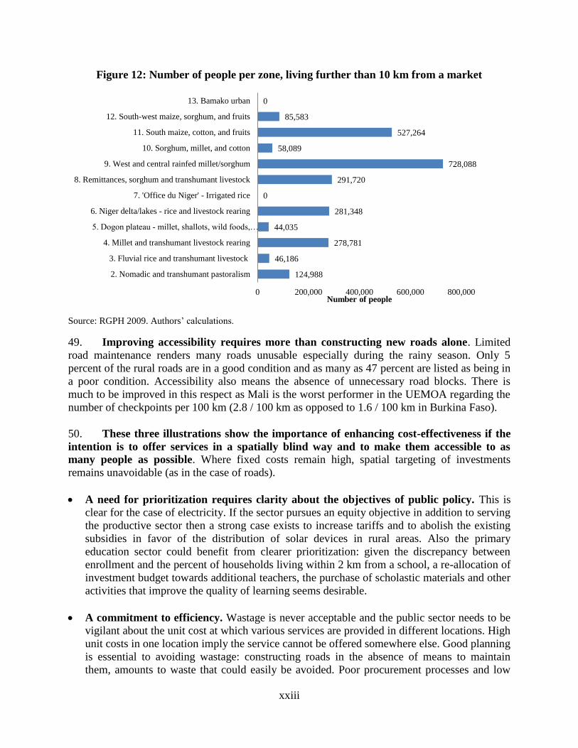
48. To assess where to prioritize improving accessibility we estimate the number of
households within each livelihood zone that do not live within 10 km of a road (Figure 12).
It suggests that despite relatively favorable access additional infrastructure in zones 9 and 11
(zones with good agricultural potential) could connect more than 1.2 million people to markets.
Also the Niger delta deserves to benefit from better access. Not only is current access poor, the
agro-ecological potential is high and the number of people that can be reached substantial.
Moreover, as will be argued in the next section, better connectivity to the Niger delta would fit
well a strategy to enhance security in north Mali through a stepwise approach.
xxiii
Figure 12: Number of people per zone, living further than 10 km from a market
Source: RGPH 2009. Authors’ calculations.
49. Improving accessibility requires more than constructing new roads alone. Limited
road maintenance renders many roads unusable especially during the rainy season. Only 5
percent of the rural roads are in a good condition and as many as 47 percent are listed as being in
a poor condition. Accessibility also means the absence of unnecessary road blocks. There is
much to be improved in this respect as Mali is the worst performer in the UEMOA regarding the
number of checkpoints per 100 km (2.8 / 100 km as opposed to 1.6 / 100 km in Burkina Faso).
50. These three illustrations show the importance of enhancing cost-effectiveness if the
intention is to offer services in a spatially blind way and to make them accessible to as
many people as possible. Where fixed costs remain high, spatial targeting of investments
remains unavoidable (as in the case of roads).
A need for prioritization requires clarity about the objectives of public policy. This is
clear for the case of electricity. If the sector pursues an equity objective in addition to serving
the productive sector then a strong case exists to increase tariffs and to abolish the existing
subsidies in favor of the distribution of solar devices in rural areas. Also the primary
education sector could benefit from clearer prioritization: given the discrepancy between
enrollment and the percent of households living within 2 km from a school, a re-allocation of
investment budget towards additional teachers, the purchase of scholastic materials and other
activities that improve the quality of learning seems desirable.
A commitment to efficiency. Wastage is never acceptable and the public sector needs to be
vigilant about the unit cost at which various services are provided in different locations. High
unit costs in one location imply the service cannot be offered somewhere else. Good planning
is essential to avoiding wastage: constructing roads in the absence of means to maintain
them, amounts to waste that could easily be avoided. Poor procurement processes and low
124,988
46,186
278,781
44,035
281,348
0
291,720
728,088
58,089
527,264
85,583
0
0 200,000 400,000 600,000 800,000
2. Nomadic and transhumant pastoralism
3. Fluvial rice and transhumant livestock
4. Millet and transhumant livestock rearing
5. Dogon plateau - millet, shallots, wild foods,…
6. Niger delta/lakes - rice and livestock rearing
7. 'Office du Niger' - Irrigated rice
8. Remittances, sorghum and transhumant livestock
9. West and central rainfed millet/sorghum
10. Sorghum, millet, and cotton
11. South maize, cotton, and fruits
12. South-west maize, sorghum, and fruits
13. Bamako urban
Number of people

xxiv
retention rates and little learning in primary school equally lead to waste that can be ill
afforded.
Unit cost reducing innovations. In a context of budgetary constraints the choice will often
be between adopting an innovation and the non-delivery of the service. To address high
student-teacher and high student - classroom ratios for example, the authorities could
consider the introduction of a double shift system in which teachers teach two classes on the
same day: one in the mornings and one in the afternoon. If a double shift system is too
demanding for the available teachers, the system could be introduced while hiring additional
teachers (maybe from neighboring countries). Instead of building schools in areas where
nomadic pastoralism is the norm, ambulant teachers who move with the people could be
considered. Identifying successful and scalable innovations and implementing these is an
important task for the public sector, particularly in an environment in which (low) population
density is such a dominant factor.
Migration. Temporary labor migration as well as permanent migration are already common,
and particularly in very low density areas, motivating people (and businesses) to move to the
service rather than the service to the people deserves to be explored as a potentially cost-
effective way of dealing with low-density problems. Policies could facilitate permanent
internal migration (of businesses and people) by reducing its cost and by increasing its
success rate (educated migrants are more likely to succeed than uneducated ones). Policies
could also facilitate temporary migration to a service such as through boarding schools or
outpatient facilities for pregnant women close to their delivery date.
51. Projections starting at 41 percent poverty in 2010, show that to reduce poverty to 20
percent by 2030 GDP growth has to reach 5.9 percent per annum. Mali’s low degree of
inequality implies that even though the incidence of poverty is high, the average distance to the
poverty line is not too large. Consequently much poverty reduction can be attained with
relatively little growth. Projections show that if the objective is to reduce poverty by half by
2030, the GDP growth rate has to reach 5.9 percent per year on average. If the objectives are
more ambitious then the average growth rate would have to be higher. Still even the target of 3
percent poverty by 2030 is attainable with a GDP growth rate that is less than 10 percent per year
on average.
52. The growth rates required to significantly reduce poverty in Mali, exceed the
growth achieved over the past two decades. As Figure 15 shows, growth rates in Mali have
fluctuated considerably over the past 20 years and rarely did they reach 5.9 percent. It implies
that halving poverty by 2030 is already an ambitious objective (the World Bank’s objective is to
reduce poverty to 3 percent) which requires a concerted effort to increase growth.

xxv
Figure 15: GDP growth rates and growth rates needed to achieve
various poverty targets by 2030
Source: Staff calculation using ELIM 2010 and IMF.
53. When it comes to designing a strategy to accelerate growth, security will need to be
restored in the north. In addition Mali’s landlocked status and the large distances to the nearest
ports need to be taken into account. Broadly speaking two growth enhancing approaches can be
envisaged: (i) a strategy that takes the high transport cost as a natural advantage; and (ii) an
export strategy for products in which Mali has a comparative advantage or for products of high
value.
Taking advantage of Mali’s landlocked status by expanding the production of cereals. The first approach is de facto being followed by the manufacturing sector, which focuses on
products that are too bulky, or too costly to be imported from elsewhere. This gives specific
local industries a local comparative advantage (production of beverages, electricity; cotton
ginning; construction). The potential for growth in this area is limited (although the
construction sector may have potential) but Mali has huge potential to export cereals to the
regional market for cereals. The Sahel is structurally food deficient (despite the increases in
cereal production even Mali imports food) and with its irrigation potential (much of which
still needs to be developed) and closeness to these markets, Mali is well placed to serve other
landlocked countries with maize, rice and other cereals. Doing so would boost poverty
reduction (i) as a strong link has been found between increasing cereal production and
reducing poverty, and (ii) as the areas with good potential for cereal production are those
where most poor people live. The poverty impact will be particularly large when poor
households are able to cultivate more land for instance because investments in human capital
improve their capacity to work (labor is the main asset of poor households) or when access to
productive assets (including irrigated land) is expanded.
Export strategy for high value added products. In the short run a growth strategy could
focus on enhanced agricultural production, but at some point the domestic and regional
16%
9%
-3%
4% 4% 2%
7%
5% 4%
6%
-3%
12%
4%
8%
2%
6% 5%
4% 5% 4%
6%
3%
0%
2%
-5%
0%
5%
10%
15%
20%
GD
P g
row
th r
ate
PIB reel objectif de 20% objectif de 10% objectif de 3%

xxvi
markets will be saturated and other sources of growth will need to be found. As domestic
demand is too limited to fuel growth and export markets will need to be tapped more
systematically. The growth potential of Mali’s main exports, cotton and gold, seems limited,
and markets will need to be developed for other products. Given the long distances to the
port, it seems unlikely that Mali will soon develop a comparative advantage in the production
of low value bulk produce, but with Paris only 5 hours away by plane, there is scope for
developing exports of high value per unit of volume or services that could be traded through
IT technology. High value products that could be considered include leather and leather
products, cut flowers, dried fruits or horticultural products. On the service side Bamako is the
music capital of West Africa, and Mali’s colorful crafts and leather work are appreciated
across the globe. Stimulating migration (and the remittances that are associated with it) and
tourism present yet another approach to exporting services. Developing any of these markets
is a long term objective requiring an educated labor force (which currently does not exist),
cheap and reliable communication and internet (does not exist) as well concerted government
action for which it is unclear whether the capacity exists.
54. Poverty can also be reduced through (cash) transfers: the potential of safety nets to
significantly reduce poverty is substantial. Reducing poverty to 3percent by 2030 would take
less than 2 percent of GDP in perfectly targeted transfers in combination with 2 percent per
capita growth (amongst the poorest households). Done well, a transfer program would not only
boost the consumption of households who are currently poor (and hence reduce their poverty),
some transfers will be invested thereby increasing productivity and enhancing growth amongst
the poor.
55. The successful implementation of these strategies will depend on applying the right
mix of spatially blind policies, policies to enhance spatial connectivity and spatially targeted
interventions. Amongst these spatially blind policies are possibly of greatest importance as
they benefit all.
Spatially blind policies are needed to create a secure environment (in the north as well as in
the rest of the country); to enhance the quality of education; to improve health services; to
provide access to the internet and cheap and reliable telecommunications; to reduce the unit
cost of service provision; to enhance the efficiency of spending; to stimulate national and
international migration (of skilled people) and to facilitate international trade. Other policies,
such as those related to the provision of electricity are presently not spatially blind, but could
be offered in a more spatially blind manner. While spatially blind are preferred,
implementation mechanisms should not be spatially blind: they need to reflect different needs
and conditions across livelihood zones.
Spatial connectivity needs to improve. To enhance economic integration and accelerate
growth travel times will need to be reduced through investments in road maintenance, a
reduction in road blocks and investments in new roads. International road connections (to
Senegal, Côte d’Ivoire, Burkina Faso and Niger) are relatively favorable (provided the roads
to Burkina Faso and Niger are secure) but within the country there remain areas with high
population density, economic potential and poor accessibility. Additional infrastructure in
zones 9 and 11 could connect another 1.2 million people to markets. Improving connectivity
xxvii
to the flood plains south of Tombouctou is equally interesting because this area has high
productive potential, is already relatively densely populated and could become the area in
which the Government of Mali demonstrates its commitment to security and its ability to
restore service delivery after the crisis.
Targeted interventions are justified and needed to reduce poverty. Where there are
pockets of deep poverty specific (spatially targeted) interventions are justified. In areas with
agricultural potential such interventions could focus on enhancing agricultural productivity
and stimulating off farm employment. Targeted interventions are equally needed in north
Mali to ensure security (from which all Malians will benefit) and to restore the delivery of
services.

1
Introduction
1.1 Space and development are intricately related.3 This is immediately clear when
considering the map of night time lights. Areas with high light intensity tend to lie in the
northern hemisphere. They also come in clusters: the east coast of the United States of America,
Europe, India and South East Asia. Areas with low levels of light intensity are also clustered: the
mid-west of the United States, the Amazon in South America, eastern China, the Sahara and,
actually, most of Africa. In areas with little light, coast lines lit up most. This is clear in South
America, the west of the United States as well as the coasts of West and Southern Africa.
1.2 Night time light intensity has been found to be a good proxy for population density
(hence the little light in the mid-west of the United States or the light in India) and for GDP per
capita (Ghosh et al. 2013).4 Thus the night time light intensity map serves to illustrate some
important spatial aspects of development. Neighborhood matters for instance. It is easier to grow
and develop if one lives near an area with great wealth. For those that do not live close to such
areas, the ability to trade goods is important, which is why the coasts are lit up.
: Night-time light intensity 2013
Source: World Bank, DECCT, 2013.
1.3 The night time light intensity map serves as reminder of some of the development
challenges Mali faces. The country only has a few bright spots of which the one associated with
3 See for instance Easterly, William and Ross Levine. (2003) "Tropics, germs, and crops: How endowments
influence economic development." Journal of Monetary Economics 2003, 50: 3-39 or Sachs, Jeffrey D. 2000.
‘Tropical Underdevelopment’. Center for International Development (CID) at Harvard University, Working Paper
No. 57. 4 Ghosh, Tilottama, Sharolyn J. Anderson, Christopher D. Elvidge and Paul C. Sutton (2013) “Using Nighttime
Satellite Imagery as a Proxy Measure of Human Well-Being”, Sustainability 2013, 5, 4988-5019.

2
Bamako is the most visible. Mali’s neighboring countries barely lit up, suggestive of being
located in a neighborhood of limited wealth due to a combination of low per capita incomes and
low population density. Mali is also far from West Africa’s ports: the distance from Bamako to
the port of Abidjan is 1,150 km, from Gao to Abidjan is 2,050 km; the distance from Bamako to
the port of Dakar is 1,400 km and from Kidal it is a whopping 2,950 km. The nearest major
market for Mali is Europe, but getting goods there requires either transporting them over long
distances of land before they can be shipped, or transporting them by air.
: Population density
Source: RGPH 2009. Authors’ calculations.
1.4 Space not only matters for patterns of development at a global scale. At a local level
space is equally important. One characteristic critical for Mali, is its low population density.
With an average population of 13.3 people per km2 Mali belongs to the 20 least densely
populated countries in the world. Averages may hide large variations and this certainly holds for
a country with vast swaths of desert where few people live. In Kidal in the north of the country,
population density is only.5 persons per square kilometer. In Tombouctou and Gao it is higher
but still low, respectively 2.0 and 3.1 people per square kilometer. In the south of the country
population density is substantially higher. It varies from 16.2 people per km2 in Kayes, to 26 in
Koulikoro and Mopti, to about 38 in Sikasso and Ségou. At over 7,400 people per square
kilometer, population density is highest in Bamako.

3
1.5 Because of the low population density, in 2009, only 9 percent of the population live in
the North of the country (Gao, Tombouctou and Kidal) even though the north comprises some 65
percent of the land mass of Mali.
1.6 Spatial differences are correlated with welfare outcomes. A person born in Bamako can
expect to live more than 6 years longer than a person born in Ségou or Sikasso. A person born in
Kidal can expect to consume almost twice as much as a person born in Mopti. A person with no
education living in Kayes can expect to consume 50 percent more than a person without
education in Sikasso, while a person with no education living in Kidal can expect to consume the
same amount as a person with an advanced degree living in Mopti.
1.7 Space is intrinsically related to geography, and as space matters, so does geography. In
Kidal, in the midst of the desert, commerce is the activity of choice, while in Sikasso with ample
fertile land available, agriculture is the primary activity. Family size is affected by geography
too. In the absence of labor markets, large families are preferred in Mali’s agricultural areas, but
less so where commerce is dominant. Hence average family size in Kayes is 12.8, but in Gao it is
8.0 and in Kidal 6.3.
1.8 These disparities in living standards and livelihoods are the outcome of a striking
attribute of economic development—its unevenness across space. This is true at all geographic
scales, from local to national to global. Cities pull ahead of the countryside. Living standards
improve in some regions while others lag. Entire countries and regions develop faster than
others. The impact of geography and space and the unevenness of development poses challenges
to decision makers who generally cannot simultaneously foster economic production and spread
it out smoothly.
1.9 The spatial differences one observes on the production side are more pronounced than
those on the welfare side. One observes that 90 percent of all formal enterprises are found in
Bamako and that an estimated 39 percent of GDP is generated in the capital city.5 Access to
services is much less skewed than production, but overall levels of access are low and spatial
differences exist: almost sixty percent of the population aged six and above has no education at
all, approximately 35 percent has primary education and slightly less than eight percent of the
population has secondary education or more.6 In the Northern regions of the country, Mopti,
Tombouctou and Kidal more than 80 percent of the population has not gone to school at all.
Contrast this with Bamako (see Figure 1.3). But even in Bamako, as many as 34 percent of the
population never went to school.
5 Note de Prospective N°6, Répartition Régionale du PIB National ou Estimation des PIB Régionaux du Mali, CAP-
Primature, Février 2014. 6 The situation in 2011 is a considerable improvement relative to 1998 when 80 percent of the population was
uneducated and less than 20 percent had gone to primary school.
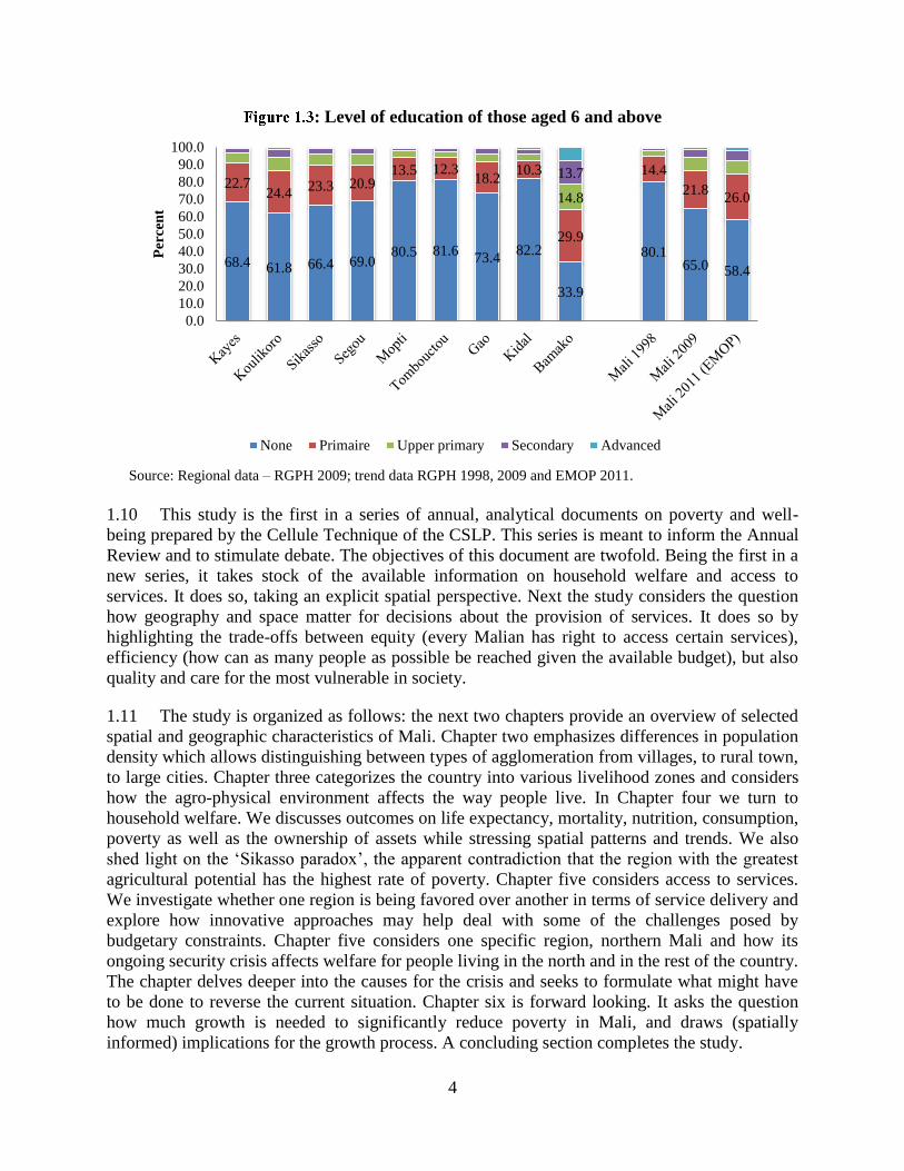
4
: Level of education of those aged 6 and above
Source: Regional data – RGPH 2009; trend data RGPH 1998, 2009 and EMOP 2011.
1.10 This study is the first in a series of annual, analytical documents on poverty and well-
being prepared by the Cellule Technique of the CSLP. This series is meant to inform the Annual
Review and to stimulate debate. The objectives of this document are twofold. Being the first in a
new series, it takes stock of the available information on household welfare and access to
services. It does so, taking an explicit spatial perspective. Next the study considers the question
how geography and space matter for decisions about the provision of services. It does so by
highlighting the trade-offs between equity (every Malian has right to access certain services),
efficiency (how can as many people as possible be reached given the available budget), but also
quality and care for the most vulnerable in society.
1.11 The study is organized as follows: the next two chapters provide an overview of selected
spatial and geographic characteristics of Mali. Chapter two emphasizes differences in population
density which allows distinguishing between types of agglomeration from villages, to rural town,
to large cities. Chapter three categorizes the country into various livelihood zones and considers
how the agro-physical environment affects the way people live. In Chapter four we turn to
household welfare. We discusses outcomes on life expectancy, mortality, nutrition, consumption,
poverty as well as the ownership of assets while stressing spatial patterns and trends. We also
shed light on the ‘Sikasso paradox’, the apparent contradiction that the region with the greatest
agricultural potential has the highest rate of poverty. Chapter five considers access to services.
We investigate whether one region is being favored over another in terms of service delivery and
explore how innovative approaches may help deal with some of the challenges posed by
budgetary constraints. Chapter five considers one specific region, northern Mali and how its
ongoing security crisis affects welfare for people living in the north and in the rest of the country.
The chapter delves deeper into the causes for the crisis and seeks to formulate what might have
to be done to reverse the current situation. Chapter six is forward looking. It asks the question
how much growth is needed to significantly reduce poverty in Mali, and draws (spatially
informed) implications for the growth process. A concluding section completes the study.
68.4 61.8 66.4 69.0 80.5 81.6
73.4 82.2
33.9
80.1 65.0 58.4
22.7 24.4
23.3 20.9 13.5 12.3
18.2 10.3
29.9
14.4
21.8 26.0 14.8
13.7
0.0
10.0
20.0
30.0
40.0
50.0
60.0
70.0
80.0
90.0
100.0P
erce
nt
None Primaire Upper primary Secondary Advanced
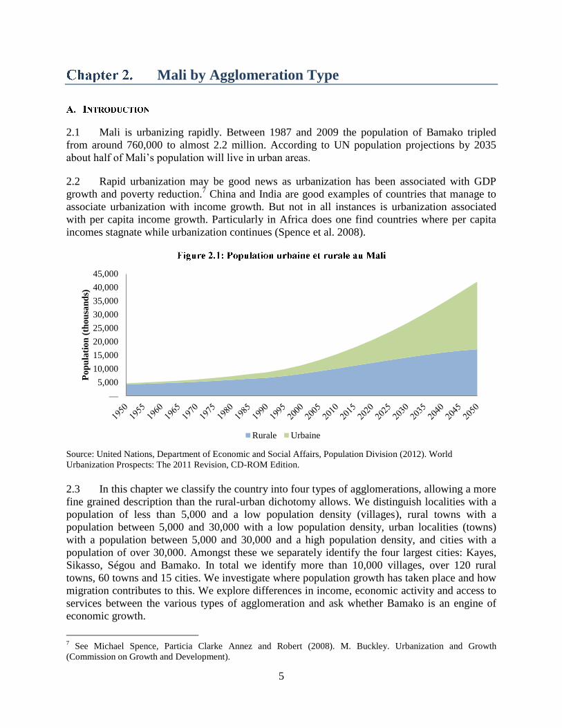
5
Mali by Agglomeration Type
2.1 Mali is urbanizing rapidly. Between 1987 and 2009 the population of Bamako tripled
from around 760,000 to almost 2.2 million. According to UN population projections by 2035
about half of Mali’s population will live in urban areas.
2.2 Rapid urbanization may be good news as urbanization has been associated with GDP
growth and poverty reduction.7 China and India are good examples of countries that manage to
associate urbanization with income growth. But not in all instances is urbanization associated
with per capita income growth. Particularly in Africa does one find countries where per capita
incomes stagnate while urbanization continues (Spence et al. 2008).
Source: United Nations, Department of Economic and Social Affairs, Population Division (2012). World
Urbanization Prospects: The 2011 Revision, CD-ROM Edition.
2.3 In this chapter we classify the country into four types of agglomerations, allowing a more
fine grained description than the rural-urban dichotomy allows. We distinguish localities with a
population of less than 5,000 and a low population density (villages), rural towns with a
population between 5,000 and 30,000 with a low population density, urban localities (towns)
with a population between 5,000 and 30,000 and a high population density, and cities with a
population of over 30,000. Amongst these we separately identify the four largest cities: Kayes,
Sikasso, Ségou and Bamako. In total we identify more than 10,000 villages, over 120 rural
towns, 60 towns and 15 cities. We investigate where population growth has taken place and how
migration contributes to this. We explore differences in income, economic activity and access to
services between the various types of agglomeration and ask whether Bamako is an engine of
economic growth.
7 See Michael Spence, Particia Clarke Annez and Robert (2008). M. Buckley. Urbanization and Growth
(Commission on Growth and Development).
—
5,000
10,000
15,000
20,000
25,000
30,000
35,000
40,000
45,000
Po
pu
lati
on
(th
ou
san
ds)
Rurale Urbaine
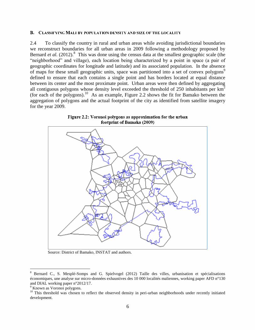
6
2.4 To classify the country in rural and urban areas while avoiding jurisdictional boundaries
we reconstruct boundaries for all urban areas in 2009 following a methodology proposed by
Bernard et al. (2012).8 This was done using the census data at the smallest geographic scale (the
“neighborhood” and village), each location being characterized by a point in space (a pair of
geographic coordinates for longitude and latitude) and its associated population. In the absence
of maps for these small geographic units, space was partitioned into a set of convex polygons9
defined to ensure that each contains a single point and has borders located at equal distance
between its center and the most proximate point. Urban areas were then defined by aggregating
all contiguous polygons whose density level exceeded the threshold of 250 inhabitants per km2
(for each of the polygons).10
As an example, Figure 2.2 shows the fit for Bamako between the
aggregation of polygons and the actual footprint of the city as identified from satellite imagery
for the year 2009.
Source: District of Bamako, INSTAT and authors.
8 Bernard C., S. Mesplé-Somps and G. Spielvogel (2012) Taille des villes, urbanisation et spécialisations
économiques, une analyse sur micro-données exhaustives des 10 000 localités maliennes, working paper AFD n°130
and DIAL working paper n°2012/17. 9 Known as Voronoi polygons.
10 This threshold was chosen to reflect the observed density in peri-urban neighborhoods under recently initiated
development.
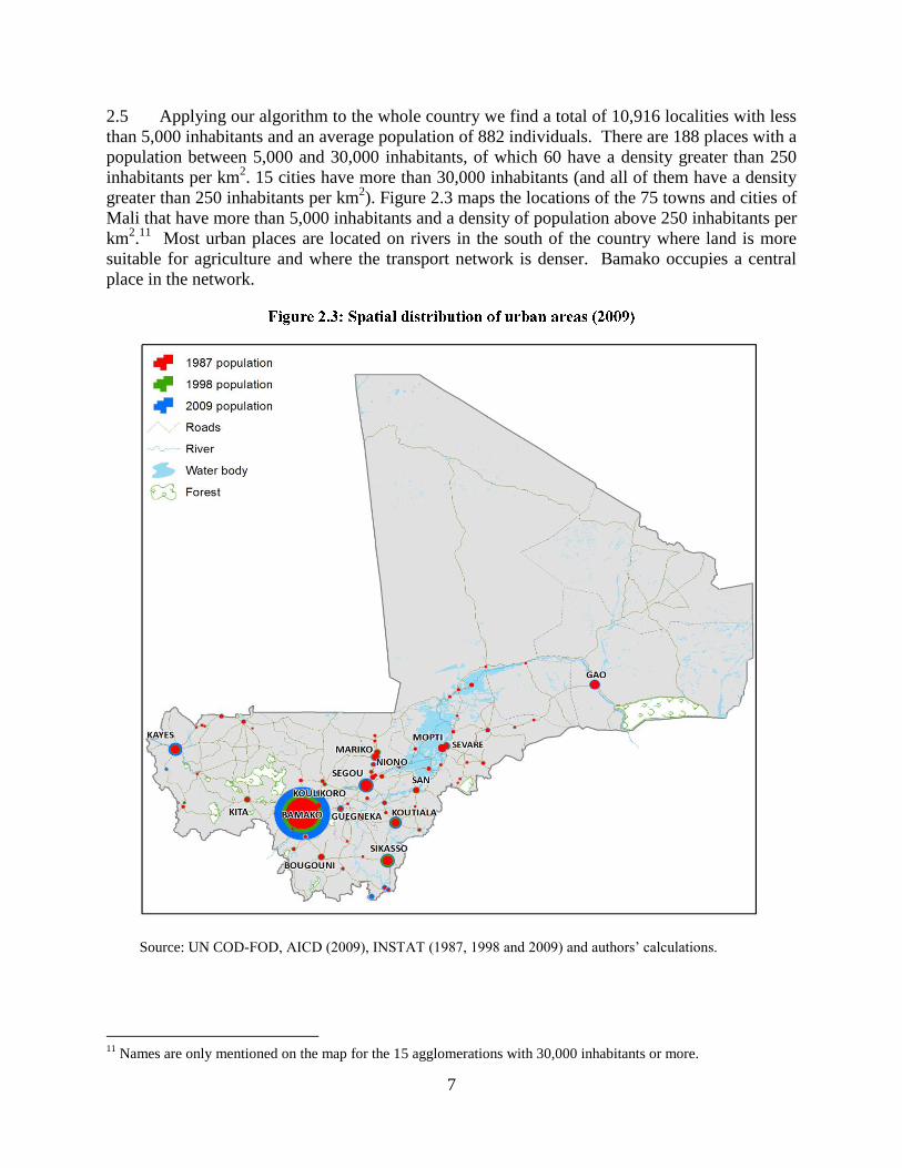
7
2.5 Applying our algorithm to the whole country we find a total of 10,916 localities with less
than 5,000 inhabitants and an average population of 882 individuals. There are 188 places with a
population between 5,000 and 30,000 inhabitants, of which 60 have a density greater than 250
inhabitants per km2. 15 cities have more than 30,000 inhabitants (and all of them have a density
greater than 250 inhabitants per km2). Figure 2.3 maps the locations of the 75 towns and cities of
Mali that have more than 5,000 inhabitants and a density of population above 250 inhabitants per
km2.11
Most urban places are located on rivers in the south of the country where land is more
suitable for agriculture and where the transport network is denser. Bamako occupies a central
place in the network.
Source: UN COD-FOD, AICD (2009), INSTAT (1987, 1998 and 2009) and authors’ calculations.
11
Names are only mentioned on the map for the 15 agglomerations with 30,000 inhabitants or more.

8
2.6 These 75 towns and cities host 3.9 million inhabitants—out of a population of 14.3
million—whereas the rest—69.5 percent of the population—resides in rural places (Figure 2.4
below).12
There is a very strong primacy of the capital city. Bamako hosts more than 2.1 million
people (15 percent of the population) whereas the three largest cities after Bamako, i.e. Ségou,
Sikasso and Kayes only host 166,000, 143,000 and 127,000 people respectively (3 percent of the
population).
Source: 2009 RGPH. Authors’ calculations.
2.7 With urbanization the size of cities can be expected to increase but the relative size
distribution typically remains unchanged. Size distributions are known to be stable over time
demonstrating how settlements of different sizes complement one another and how within a
country a wide range of city sizes coexist. The size-rank rule associates the population of any
city to the population of the largest city, divided by the rank of the city in question within the
country’s urban hierarchy. This rank-size rule, discovered in 1913, can be expressed as the rank r
associated with a city of size S is proportional to S to some negative power (World Bank 2009).13
The rule holds in Mali. Ranking cities from largest to smallest and comparing their sizes with
those predicted by the rank rule, one finds a closeness (the scale factor is 0.88 –suggesting a
strong dominance of the largest city) and a stable relation over time.
2.8 Despite the stability of the relation, the ranking of cities did change over time. Bamako
remains by far the largest city but Ségou and Sikasso have switched places: Sikasso took over
second place from Ségou in 1998 but lost it in 2009. Kayes remains in fourth rank (Table 2.1).
12
We define rural areas as places with less than 5,000 residents or with a population density below 250 people per
km2.
13 World Bank 2009. World Development Report 2009: Reshaping Economic Geography.
66% 7%
5%
4%
1%
1%
1% 15% population <5,000
population [5,000-30,000[, density<250 people/km2
population [5,000-30,000[, density>=250 people/km2
population >=30,000, density>=250 people/km2
Kayes
Sikasso
Ségou
Bamako

9
City rank
City size
1987
City size
1998
City size
2009
1 Bamako 757,051 Bamako 1,132,886 Bamako 2,156,177
2 Ségou 88,714 Sikasso 109,570 Ségou 166,128
3 Sikasso 69,840 Ségou 91,882 Sikasso 143,231
4 Kayes 58,720 Kayes 71,897 Kayes 127,473
Source: RGPH for 1998 and 2009, authors’ calculations.
2.9 Disproportionate primacy of the capital city is often a characteristic of developing
economies (Glaeser and Ades, 1994).14
There can be various reasons for such primacy (see
Overman and Venables, 2005);15
we suspect that the main ones explaining the lack of
specialization of cities and the dominance of Bamako have to do with the centralization of
political power, long distances between cities, the poor quality of the intercity transport and
communication network contributing to high communication and transport cost.
2.10 Interestingly, and unexpectedly, we find that demographic characteristics are not very
different between rural and urban areas. The average proportion of children in villages, for
instance, in towns (with a population below 30,000 inhabitants) and in cities (with a population
larger than 30,000) stands at 48.4 percent, 45.5 percent and 43.6 percent respectively in 2009
(see Annex, Table 3).16
It is only in the two biggest cities (Ségou and Bamako) where the
proportion of children falls below 40 percent (with 39.3 percent in Ségou and 38.9 percent in
Bamako).17
2.11 Average household size remains very high throughout Mali. Remarkably, as Table 2.2
demonstrates household size increases with the degree of urbanization. Average household size
is 8.1 in villages, between 8.7 and 8.9 in towns and more than 9 in the largest cities. This is
explained by the fact that urban households are more likely to accommodate extended family
members than rural households: although the average proportion of extended family members in
rural households is already high at 39.7 percent, it reaches about 50.0 percent in cities. This
difference is partially due to the presence of students and adults looking for jobs in medium sized
cities and in Bamako (as illustrated by the economic dependency ratios and the proportions of
student household members in Table 2.2).
2.12 Both push factors such as poor living conditions, weather, insecurity or other shocks and
limited economic opportunities in rural areas as well as pull factors may explain why so many
migrate to urban areas. In view of our spatial analysis of economic activities (see the next
14
Glaeser, E. and A. Ades (1994) Trade and Circuses: Explaining Urban Giants, Quarterly Journal of Economics,
110(1), 195-227. 15
Overman, H.G. and A.J. Venables (2005) “Cities in the Developing World”, CEP Discussion paper 695. 16
The demographic dependency ratio, however, ranks inversely as it is much lower in urban than in rural areas. (see
table 2.2). 17
The gap between Bamako and rural areas in the proportion of children (almost 10 percentage points) was actually
negative (-0.7 percentage points) in 1987 and only +7 percentage point in 1998, showing that the demographic
transition started very late in Mali, even in Bamako (see tables Annex 2.1 and Annex 2.2).
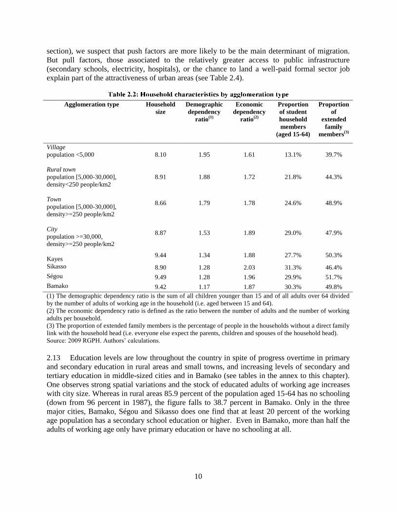
10
section), we suspect that push factors are more likely to be the main determinant of migration.
But pull factors, those associated to the relatively greater access to public infrastructure
(secondary schools, electricity, hospitals), or the chance to land a well-paid formal sector job
explain part of the attractiveness of urban areas (see Table 2.4).
Agglomeration type Household
size
Demographic
dependency
ratio(1)
Economic
dependency
ratio(2)
Proportion
of student
household
members
(aged 15-64)
Proportion
of
extended
family
members(3)
Village
population <5,000
8.10 1.95 1.61 13.1% 39.7%
Rural town
population [5,000-30,000],
density<250 people/km2
8.91 1.88 1.72 21.8% 44.3%
Town
population [5,000-30,000],
density>=250 people/km2
8.66 1.79 1.78 24.6% 48.9%
City
population >=30,000,
density>=250 people/km2
8.87 1.53 1.89 29.0% 47.9%
Kayes 9.44 1.34 1.88 27.7% 50.3%
Sikasso 8.90 1.28 2.03 31.3% 46.4%
Ségou 9.49 1.28 1.96 29.9% 51.7%
Bamako 9.42 1.17 1.87 30.3% 49.8%
(1) The demographic dependency ratio is the sum of all children younger than 15 and of all adults over 64 divided
by the number of adults of working age in the household (i.e. aged between 15 and 64).
(2) The economic dependency ratio is defined as the ratio between the number of adults and the number of working
adults per household.
(3) The proportion of extended family members is the percentage of people in the households without a direct family
link with the household head (i.e. everyone else expect the parents, children and spouses of the household head).
Source: 2009 RGPH. Authors’ calculations.
2.13 Education levels are low throughout the country in spite of progress overtime in primary
and secondary education in rural areas and small towns, and increasing levels of secondary and
tertiary education in middle-sized cities and in Bamako (see tables in the annex to this chapter).
One observes strong spatial variations and the stock of educated adults of working age increases
with city size. Whereas in rural areas 85.9 percent of the population aged 15-64 has no schooling
(down from 96 percent in 1987), the figure falls to 38.7 percent in Bamako. Only in the three
major cities, Bamako, Ségou and Sikasso does one find that at least 20 percent of the working
age population has a secondary school education or higher. Even in Bamako, more than half the
adults of working age only have primary education or have no schooling at all.

11
Source: RGPH 2009. Authors’ calculations.
2.14 Levels of interregional migration18
are high and an important contributor to city growth.
Bamako and Koulikoro are net recipients of migrants, while the regions of Ségou, Mopti,
Tombouctou and Gao are the largest net contributors of migrants. Levels of intra-regional
migration are relatively marginal: migrants go to urban areas, and less to other (rural) localities
in their region of origin.
Source: Source: RGPH 2009. Authors’ calculations.
2.15 Migrants tend to be better educated than the average person (Figure 2.6), but relative to
the average person living in Bamako, migrants are less well educated: about 6 percent of people
18
Here we mean permanent migration in which one changes his or her main residence and not temporary labor
migration.
-1.1
3.1
-1.1
-4.6 -3.5
-5.1 -3.9
-0.1
11.6
-6.00
-4.00
-2.00
0.00
2.00
4.00
6.00
8.00
10.00
12.00
14.00P
erce
nt
55.13
71.8
33.9
65.29
29.34 24.9
44.7
28.72
15.50
3.3
21.5
6.00
0.00
10.00
20.00
30.00
40.00
50.00
60.00
70.00
80.00
Average migrant Average returnee Average person in
Bamako
Average person in Mali
Per
cen
t
None Primary Secondary and above

12
in Mali have a secondary education but 15 percent of the migrants have one. Better educated
migrants have a greater likelihood of success and poorly educated migrants are more likely to
return: amongst the returning migrants one finds few people with a secondary education (3
percent) while the vast majority (72 percent) has no education.
Agglomeration type No
school
Primary Second. 1 Second. 2 Tertiary All
migrants
Village
population < 5000 20.5% 10.8% 8.5% 6.6% 3.9% 14.6%
Rural town
population [5,000-30,000],
density<250 people/km2
4.3% 4.6% 4.3% 3.9% 2.6% 4.2%
Town
population [5,000-30,000],
density>=250 people/km2
7.1% 6.6% 7.0% 6.1% 4.0% 6.6%
City (excl. KBSS)
population >=30,000,
density>=250 people/km2
8.0% 9.4% 10.5% 11.0% 6.6% 8.8%
Kayes 1.6% 2.2% 2.0% 2.1% 1.1% 1.7%
Sikasso 1.3% 1.7% 1.9% 2.1% 1.2% 1.6%
Ségou 1.5% 2.1% 2.7% 2.9% 1.7% 1.9%
Bamako 55.5% 62.7% 63.1% 65.4% 78.9% 60.5%
100% 100% 100% 100% 100% 100%
Total number of migrants 525,874 135,114 102,019 138,041 77,921 978,969
Source: 2009 RGPH. Authors’ calculations.
2.16 The strong migration selection according to level of education is illustrated by Table 2.3
which shows that skilled migrants are found in higher proportions in medium-sized cities and in
Bamako.19
Whereas 60.5 percent of all internal migrants are located in Bamako, the city hosts a
disproportionate share of migrants with a tertiary education (78.9 percent). In contrast,
Bamako’s share of migrants with no education is below the national average (55.5 percent).
Whereas 24.5 percent of uneducated migrants are in rural areas, only 10.9 percent and 6.5
percent of those with a high school or a tertiary education respectively migrate to rural areas.
These patterns are likely to reflect relatively better opportunities for skilled workers and possibly
higher returns to education in cities.
19
Table 2 breaks down internal migration destinations by educational level for the stock of migrants in 2009. We
are not able, however, to distinguish whether migrants acquired education before or after migrating.

13
Table 2.4: Access to
basic utilities
(2009)Agglomeration type
Households
whose main
supply of
water is from a
faucet
Households
whose main
supply of
water is from
a well or bore
hole
Proportion
of
households
with
electricity
Proportion
of
households
with toilets
Proportion
of
households
using
latrines
Village
population <5,000 1.8% 87.5% 1.1% 5.7% 61.7%
Rural town
population [5,000-30,000],
density<250 people/km2 12.9% 67.9% 8.1% 7.6% 73.2%
Town
population [5,000-30,000],
density>=250 people/km2 15.8% 69.1% 17.1% 7.0% 81.6%
City
population >=30,000,
density>=250 people/km2 32.5% 54.1% 42.2% 10.1% 83.7%
Kayes 60.1% 8.2% 50.7% 14.5% 81.3%
Sikasso 43.8% 50.7% 48.6% 11.3% 84.5%
Ségou 23.0% 63.8% 47.0% 11.9% 83.2%
Bamako 40.1% 34.3% 68.2% 21.3% 74.1%
Number of
schools
Number of
health centers
Schools
(per '000
residents)
Health centers
(per '000 residents)
Village
population <5,000
0.74 0.15 0.96 0.12
Rural town
population [5,000-30,000],
density<250 people/km2
6.06 1.55 0.40 0.15
Town
population [5,000-30,000],
density>=250 people/km2
6.28 1.38 0.55 0.12
City
population >=30,000,
density>=250 people/km2
22.73 5.27 0.47 0.10
Kayes
53.00 7.00 0.37 0.05
Sikasso 70.00 13.00 0.46 0.08
Ségou 96.00 9.00 0.58 0.05
Bamako 1,182.00 206.00 0.54 0.09
Source: 2009 RGPH. Authors’ calculations.
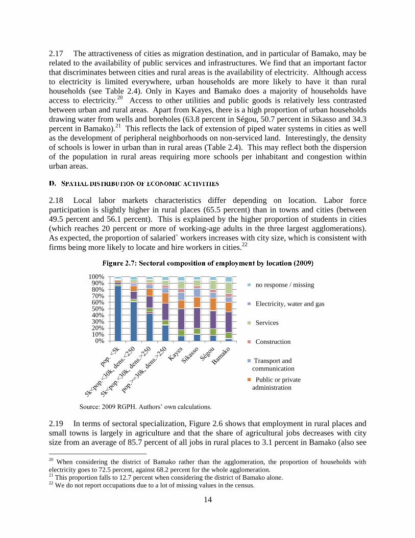
14
2.17 The attractiveness of cities as migration destination, and in particular of Bamako, may be
related to the availability of public services and infrastructures. We find that an important factor
that discriminates between cities and rural areas is the availability of electricity. Although access
to electricity is limited everywhere, urban households are more likely to have it than rural
households (see Table 2.4). Only in Kayes and Bamako does a majority of households have
access to electricity.20
Access to other utilities and public goods is relatively less contrasted
between urban and rural areas. Apart from Kayes, there is a high proportion of urban households
drawing water from wells and boreholes (63.8 percent in Ségou, 50.7 percent in Sikasso and 34.3
percent in Bamako).21
This reflects the lack of extension of piped water systems in cities as well
as the development of peripheral neighborhoods on non-serviced land. Interestingly, the density
of schools is lower in urban than in rural areas (Table 2.4). This may reflect both the dispersion
of the population in rural areas requiring more schools per inhabitant and congestion within
urban areas.
2.18 Local labor markets characteristics differ depending on location. Labor force
participation is slightly higher in rural places (65.5 percent) than in towns and cities (between
49.5 percent and 56.1 percent). This is explained by the higher proportion of students in cities
(which reaches 20 percent or more of working-age adults in the three largest agglomerations).
As expected, the proportion of salaried` workers increases with city size, which is consistent with
firms being more likely to locate and hire workers in cities.22
Source: 2009 RGPH. Authors’ own calculations.
2.19 In terms of sectoral specialization, Figure 2.6 shows that employment in rural places and
small towns is largely in agriculture and that the share of agricultural jobs decreases with city
size from an average of 85.7 percent of all jobs in rural places to 3.1 percent in Bamako (also see
20
When considering the district of Bamako rather than the agglomeration, the proportion of households with
electricity goes to 72.5 percent, against 68.2 percent for the whole agglomeration. 21
This proportion falls to 12.7 percent when considering the district of Bamako alone. 22
We do not report occupations due to a lot of missing values in the census.
0%10%20%30%40%50%60%70%80%90%
100%
no response / missing
Electricity, water and gas
Services
Construction
Transport and
communication
Public or private
administration
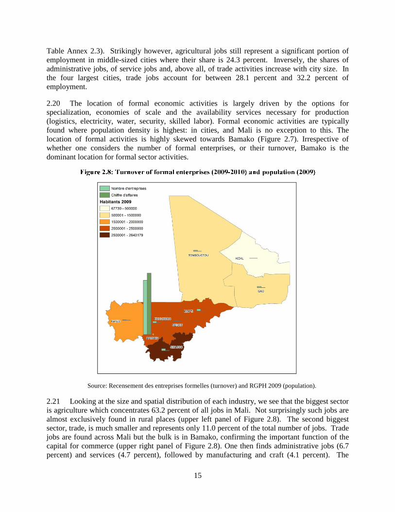
15
Table Annex 2.3). Strikingly however, agricultural jobs still represent a significant portion of
employment in middle-sized cities where their share is 24.3 percent. Inversely, the shares of
administrative jobs, of service jobs and, above all, of trade activities increase with city size. In
the four largest cities, trade jobs account for between 28.1 percent and 32.2 percent of
employment.
2.20 The location of formal economic activities is largely driven by the options for
specialization, economies of scale and the availability services necessary for production
(logistics, electricity, water, security, skilled labor). Formal economic activities are typically
found where population density is highest: in cities, and Mali is no exception to this. The
location of formal activities is highly skewed towards Bamako (Figure 2.7). Irrespective of
whether one considers the number of formal enterprises, or their turnover, Bamako is the
dominant location for formal sector activities.
Source: Recensement des entreprises formelles (turnover) and RGPH 2009 (population).
2.21 Looking at the size and spatial distribution of each industry, we see that the biggest sector
is agriculture which concentrates 63.2 percent of all jobs in Mali. Not surprisingly such jobs are
almost exclusively found in rural places (upper left panel of Figure 2.8). The second biggest
sector, trade, is much smaller and represents only 11.0 percent of the total number of jobs. Trade
jobs are found across Mali but the bulk is in Bamako, confirming the important function of the
capital for commerce (upper right panel of Figure 2.8). One then finds administrative jobs (6.7
percent) and services (4.7 percent), followed by manufacturing and craft (4.1 percent). The
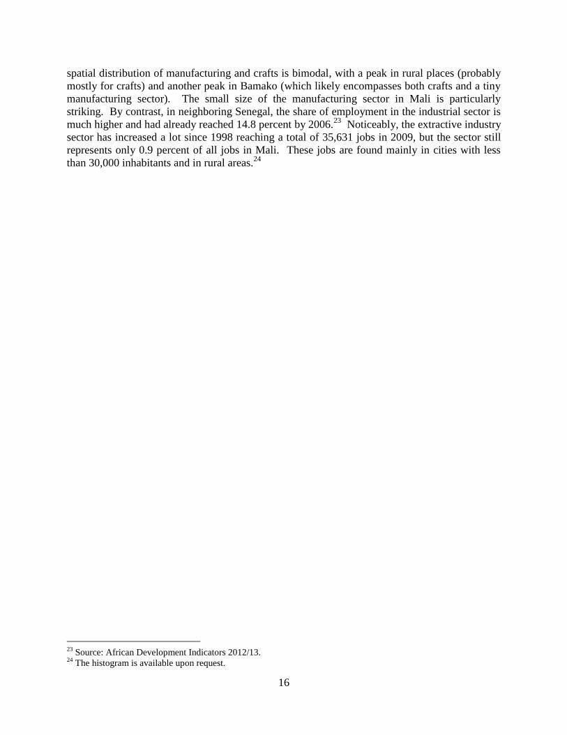
16
spatial distribution of manufacturing and crafts is bimodal, with a peak in rural places (probably
mostly for crafts) and another peak in Bamako (which likely encompasses both crafts and a tiny
manufacturing sector). The small size of the manufacturing sector in Mali is particularly
striking. By contrast, in neighboring Senegal, the share of employment in the industrial sector is
much higher and had already reached 14.8 percent by 2006.23
Noticeably, the extractive industry
sector has increased a lot since 1998 reaching a total of 35,631 jobs in 2009, but the sector still
represents only 0.9 percent of all jobs in Mali. These jobs are found mainly in cities with less
than 30,000 inhabitants and in rural areas.24
23
Source: African Development Indicators 2012/13. 24
The histogram is available upon request.
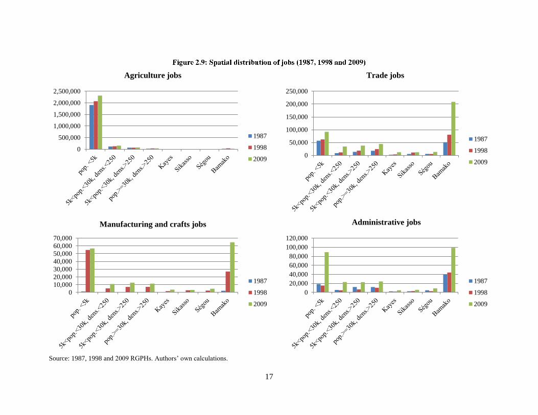
17
Agriculture jobs
Trade jobs
Manufacturing and crafts jobs Administrative jobs
Source: 1987, 1998 and 2009 RGPHs. Authors’ own calculations.
0
500,000
1,000,000
1,500,000
2,000,000
2,500,000
1987
1998
20090
50,000
100,000
150,000
200,000
250,000
1987
1998
2009
0
10,000
20,000
30,000
40,000
50,000
60,000
70,000
1987
1998
2009
0
20,000
40,000
60,000
80,000
100,000
120,000
1987
1998
2009

18
2.22 In terms of GDP the primary sector contributes about 25 percent. The contributions of the
secondary and tertiary sectors are about equal: 38 and 37 percent respectively (Figure 2.9).
Regions where the primary sector is largest contributor to income (Mopti, Ségou , Sikasso,
Koulikoro, Tombouctou and Gao) are those with the lowest GDP per capita. Regions where the
secondary and tertiary sectors are the important contributors to GDP (Kayes and Bamako) have
much higher levels of GDP per capita. The differences are striking. GDP per capita in Bamako is
five times more than that in Sikasso and eight times more than in Mopti. It illustrates the much
higher levels of productivity that are attained in the secondary and tertiary sectors than in the
primary.
2.23 The dominance of Bamako in generating income is such that with 15 percent of the
population about 40 percent of GDP is generated in the capita city. With 18 percent, Kayes is
another important contributor to GDP followed by Sikasso (12 percent) and Kouliloro (11
percent). It is no coincidence that the region with the highest levels of GDP per capita (Bamako)
is also the region with the largest urban population. The strong correlation between population
density and economic mass is consistent with urban areas being a conglomeration of consumers
and producers and possibly marks the presence of a virtuous cycle where the areas with the
highest contribution to GDP, attract most people.
Source: Repartition Regionale de la Population, de la Production et de la Consommation au Mali. Authors’
calculations.
25%
38% 37%
18%
11% 12% 9%
5% 2% 2% 1%
40%
$635
$312 $311 $273 $187
$243 $306
$782
$1,554
$486
$-
$200
$400
$600
$800
$1,000
$1,200
$1,400
$1,600
$1,800
0%
10%
20%
30%
40%
50%
60%
GD
P p
er c
ap
ita
Sh
are o
f G
DP
Primaire Secondaire Tertiaire PIB PIB par habitant (US$ 2005)

19
2.24 Using three waves of census data (1987, 1998 and 2009), we are able to characterize
urban population growth holding the spatial extent of agglomerations constant at their 2009
levels. We find that the population of Bamako grew on average at 4.9 percent annually over the
period 1987-2009, with an acceleration over the period 1998-2009, when it grew at an extremely
high annual average of 6.1 percent.25
By contrast, secondary cities and places in rural areas grew
at lower rates (3.6 percent and 2.3 percent respectively over 1987-2009).
2.25 In spite of the lower rural population growth rate, because Mali remains predominantly
rural, the population in rural locations grew by more than 4.1 million residents between 1987 and
2009 while the population of all towns and cities (defined as places with a density above 250
people per km2) “only” grew by 2.2 million. Hence cities and towns only contributed to 30.5
percent of the total population increase over the period whereas the bulk of the population
increase came from rural areas with a total contribution of 69.5 percent. Because cities grew at a
faster pace than rural areas Mali urbanized over the period. The urban population as we defined
it more than doubled between 1987 and 2009 (+129 percent).
2.26 Urbanization is believed to contribute to higher incomes through multiple channels.
Process industries, such as chemicals or steel operate more effectively at higher volumes; for this
reason they have traditionally establish in urban areas. Specialized services—such as accounting
or tax advice are easier to obtain in large cities. Specialization among input producers may allow
cost reductions, making local purchasers of their inputs more productive. Particularly in
countries with poor transportation and communication infrastructure are these important
advantages of agglomeration. Public services such as hospitals or sports stadiums also require a
minimum number of consumers to be economically viable.
2.27 High densities in cities allow workers with differentiated skills and firms with specific
needs to reduce their search costs and agglomeration effects in cities affect knowledge sharing.
By bringing together large numbers of people, cities facilitate the kinds of face to face
interactions needed to generate, diffuse, and accumulate knowledge, especially in industries that
experience rapid technological change.
2.28 Despite these various reasons as to why urbanization may lead to higher incomes we find
no clear association between urbanization and per capita incomes. This is illustrated in Figure
2.10 which shows, using World Bank data, how prior to the year 1995, the correlation between
urbanization and GDP was very weak: GDP per capita stagnated while urbanization continued.
Since the mid-1990s up to 2010 urbanization and GDP per capita appear to move in parallel. The
latest data suggest continued urbanization but stagnating GDP per capita.
25
Because the administrative definition of Bamako excludes peripheral areas that were progressively incorporated
into the agglomeration, our measure is greater than the official population figure of only 1.8 million for the six
communes that form the Bamako district (core urban area).
20
Source: World Development Indicators 2013.
2.29 An (indirect) way to get a sense as to whether urbanization is a driver of economic
growth is by checking how much rural-urban migration contributes to poverty reduction. If
structural transformation is taking place and people move from low productivity agriculture into
higher productive occupations in urban areas, then a rural-urban population shift can be expected
to contribute to poverty reduction. We find little evidence for this. Decomposing the change in
poverty that occurred between 2001 and 2010 (a decline by 9.9 percentage points) one finds that
most of this change (9.4 percent) was due to a reduction in poverty amongst people who
continued to reside in their location of origin. The contribution of people who shift from rural to
urban areas is tiny: 0.3 percent (Table 2.5).
Change in poverty -9.93%
of which: change of people who remained resident -9.37%
of which rural-urban migration -0.33%
.. of which interaction effect -0.23%
Source: EMEP 2001 and ELIM 2010. Authors’ calculations.
2.30 The contribution of Bamako proper to national poverty reduction is also very limited: 0.7
percent. This comes as no surprise because between 2001 and 2010 per capita consumption
levels remained more or less unchanged (at FCFA 279,000 per capita). That poverty fell none the
less from 14 percent on 2001 to 8 percent in 2010 is because poor households benefited from
(albeit) low levels of positive per capita growth while the wealthiest households started
consuming less. This is illustrated with the growth incidence curves for Bamako (Figure 2.11). A
growth incidence curve shows for every percentile in the consumption distribution the
(annualized) percentage change in consumption.
2.31 The Figure illustrates how over the period 2001-2010 per capita consumption growth
hovered around 1 percent per annum for most households, except for the top 10 percent who
became less well off. If one decomposes the overall change in two period, 2001-2006 and 2006-
0
5
10
15
20
25
30
35
0
100
200
300
400
500
600
Urb
an
po
pu
lati
on
GD
P p
er c
ap
ita
GDP per capita (constant 2005 US$) Urban population (% of total)
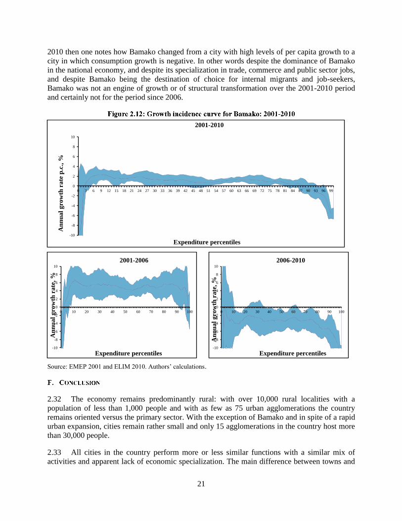
21
2010 then one notes how Bamako changed from a city with high levels of per capita growth to a
city in which consumption growth is negative. In other words despite the dominance of Bamako
in the national economy, and despite its specialization in trade, commerce and public sector jobs,
and despite Bamako being the destination of choice for internal migrants and job-seekers,
Bamako was not an engine of growth or of structural transformation over the 2001-2010 period
and certainly not for the period since 2006.
Source: EMEP 2001 and ELIM 2010. Authors’ calculations.
2.32 The economy remains predominantly rural: with over 10,000 rural localities with a
population of less than 1,000 people and with as few as 75 urban agglomerations the country
remains oriented versus the primary sector. With the exception of Bamako and in spite of a rapid
urban expansion, cities remain rather small and only 15 agglomerations in the country host more
than 30,000 people.
2.33 All cities in the country perform more or less similar functions with a similar mix of
activities and apparent lack of economic specialization. The main difference between towns and
-10
-8
-6
-4
-2
0
2
4
6
8
10
0 3 6 9 12 15 18 21 24 27 30 33 36 39 42 45 48 51 54 57 60 63 66 69 72 75 78 81 84 87 90 93 96 99
An
nu
al
gro
wth
ra
te p
.c.,
%
Expenditure percentiles
2001-2010
-10
-8
-6
-4
-2
0
2
4
6
8
10
0 10 20 30 40 50 60 70 80 90 100
An
nu
al
gro
wth
ra
te, %
Expenditure percentiles
2001-2006
-10
-8
-6
-4
-2
0
2
4
6
8
10
0 10 20 30 40 50 60 70 80 90 100
An
nu
al
gro
wth
ra
te, %
Expenditure percentiles
2006-2010

22
cities is the smaller share of the agricultural sector in cities which is replaced by a larger share of
the trade, public, and service sectors, but not by a manufacturing sector. The lack of
specialization suggests that the cities are not well connected among themselves, possibly due to
long distances and the poor quality of roads resulting in high transport and communication costs.
2.34 The manufacturing sector, although more present in larger urban areas, remains small,
even in Bamako. There is no evidence of the manufacturing sector expanding rapidly and the
share of the population working in manufacturing and crafts in Bamako has remained unchanged
since 1998 (while the trade and transport sectors have gained in importance, at the expense of
services and the public sector).
(*) Excludes those working in agriculture and non-responses.
Source: RGPH 1988 and 2009.
2.35 These traits –coupled with the observation that per capita incomes have not been growing
since 2001 are suggestive of an economy where agglomeration is not accompanied by structural
transformation towards productive industrial and services sectors and where a scattered urban
population of modest skills and modest incomes does not generate sufficient market size to boost
the demand for transformed goods or for high value-added services and does not provide the
educated workforce necessary for the development of such activities.26
It should equally be
noted as there is potential for development in rural areas through commercial agriculture and
better exploitation of mining resources, this requires functioning cities with adequate
infrastructure for transit and export. At present this does not seem to be the case. Instead the
relatively greater wealth of households in Bamako reflects more the sorting of educated workers
into the city and into greater opportunities for rent capture than true agglomeration effects
whereby density would be associated with higher productivity.
2.36 While Mali is likely to continue to urbanize, it will be important to reflect on the set of
policies that can address the deficiencies that prevent urbanization from being conducive to
sustained growth.
26
Substantial structural population shifts without growth has been coined “pathological urbanization”, a term that
seems to be applicable to Mali.
0%
11%
33%
0%
18%
8% 5%
23%
1% 0%
11%
36%
1%
17%
9% 6%
19%
1%
0%5%
10%15%20%25%30%35%40%
Per
cen
t
1988 2009
23
Mali by Livelihood Zone
3.1 In the previous chapter we classified the country by agglomeration based on population
density. In this chapter we introduce another type of classification: by economic activity or
livelihood. Agro-ecology is an important determinant of livelihood, and since this factor is
spatially correlated, it is possible to divide the country into a number of livelihood zones, defined
as areas within which people share broadly the same production system.
3.2 We follow a classification developed by FEWSNET (2010) based on an elaborate
research using key-informant interviews and stakeholder discussions. It identifies 13 livelihood
zones. We borrow extensively from the document FEWSNET produced to describe these
different zones.27
3.3 Livelihood zone boundaries do not follow administrative boundaries. One finds, for
instance, three different patterns of livelihood in Sikasso. But at finer administrative levels –the
commune, livelihood zones are defined by administrative boundaries. This makes it possible,
using geographic matching tools, to combine livelihood zone information with data from other
sources such as the population censuses and the various household surveys. This information is
used to complement the analysis presented by FEWSNET.
3.4 Rainfall is a decisive factor in identifying livelihood zones. Levels of rainfall help
explain the degree of dependence on livestock herding and the uses to which arable land can be
put. Rainfall levels vary from very low in the desert in the far north (receiving under 200mm of
precipitation per year) to between 1,000 and 1,300mm per year in the lusher zones in the south.
Following the broad rainfall pattern, 12 rural livelihood zones plus Bamako are distinguished
(see Figure 3.1 for their location)
3.5 Zone 1 represents the desert, an area of low population density in which nomadism and
commerce are the dominant activities. Kidal lies in zone 1. Like zone 1, zone 2 does not receive
sufficient rainfall to support rain fed agriculture: it is where nomadic and transhumant
pastoralism are the dominant activity. Gao and Tombouctou are the main urban centers in this
zone, even though strictly speaking both lie in the fluvial basin of the Niger river which is
classified as livelihood zone 3. The higher precipitation in zone 4 -the wide Sahelian band-
allows cultivation of millet and cowpeas, but low and unreliable levels of rainfall means that
depending on agriculture alone is risky. It explains why transhumant livestock rearing is an
important activity in this zone.
3.6 Zone 9, the band stretching roughly from Kayes to Bamako to Ségou represents a
transition from the north to the south; there is a decreasing dependence on livestock and an
increasingly diverse range of food and cash crops that are being grown. With increasing
agricultural potential, family size and population density increase. The three southern-most zones
27
FEWSNET 2010: Livelihood Zoning and Profiling Report: Mali.

24
(10, 11, 12) which are demarcated by Bamako to the north and Sikasso to the south, are not only
highly productive with the largest range of crops grown, these are also the zones with the largest
families and greatest population density.
Source: FEWSNET 2010.
3.7 The Niger river defines another three livelihood zones. The delta (zone 6) near Mopti is a
vast flood plain that is inundated for five months of the year; flooding is facilitated by another
factor - the very low slope of the ground, which allows the waters to spread out. This creates a
major resource in terms of pasture and allows households to cultivate rice and sorghum. The
river also defines the livelihoods of households living along its banks (zone 3) from the north of
the delta to the international border between Mali and Niger, where irrigated rice is a particular
feature. In a still more direct way, Bozo fishermen (representing a subzone in zone 6), who
operate along the length of the river, are dependent on it for survival. Finally the Office du Niger
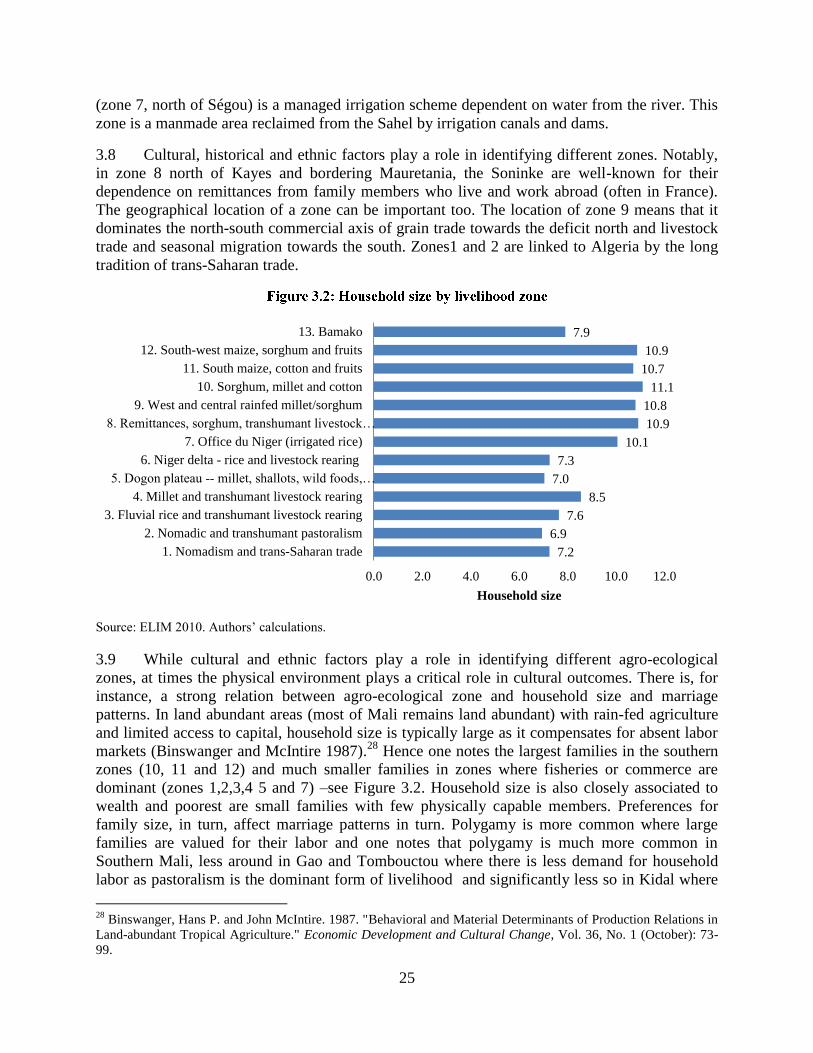
25
(zone 7, north of Ségou) is a managed irrigation scheme dependent on water from the river. This
zone is a manmade area reclaimed from the Sahel by irrigation canals and dams.
3.8 Cultural, historical and ethnic factors play a role in identifying different zones. Notably,
in zone 8 north of Kayes and bordering Mauretania, the Soninke are well-known for their
dependence on remittances from family members who live and work abroad (often in France).
The geographical location of a zone can be important too. The location of zone 9 means that it
dominates the north-south commercial axis of grain trade towards the deficit north and livestock
trade and seasonal migration towards the south. Zones1 and 2 are linked to Algeria by the long
tradition of trans-Saharan trade.
Source: ELIM 2010. Authors’ calculations.
3.9 While cultural and ethnic factors play a role in identifying different agro-ecological
zones, at times the physical environment plays a critical role in cultural outcomes. There is, for
instance, a strong relation between agro-ecological zone and household size and marriage
patterns. In land abundant areas (most of Mali remains land abundant) with rain-fed agriculture
and limited access to capital, household size is typically large as it compensates for absent labor
markets (Binswanger and McIntire 1987).28
Hence one notes the largest families in the southern
zones (10, 11 and 12) and much smaller families in zones where fisheries or commerce are
dominant (zones 1,2,3,4 5 and 7) –see Figure 3.2. Household size is also closely associated to
wealth and poorest are small families with few physically capable members. Preferences for
family size, in turn, affect marriage patterns in turn. Polygamy is more common where large
families are valued for their labor and one notes that polygamy is much more common in
Southern Mali, less around in Gao and Tombouctou where there is less demand for household
labor as pastoralism is the dominant form of livelihood and significantly less so in Kidal where
28
Binswanger, Hans P. and John McIntire. 1987. "Behavioral and Material Determinants of Production Relations in
Land-abundant Tropical Agriculture." Economic Development and Cultural Change, Vol. 36, No. 1 (October): 73-
99.
7.2
6.9
7.6
8.5
7.0
7.3
10.1
10.9
10.8
11.1
10.7
10.9
7.9
0.0 2.0 4.0 6.0 8.0 10.0 12.0
1. Nomadism and trans-Saharan trade
2. Nomadic and transhumant pastoralism
3. Fluvial rice and transhumant livestock rearing
4. Millet and transhumant livestock rearing
5. Dogon plateau -- millet, shallots, wild foods,…
6. Niger delta - rice and livestock rearing
7. Office du Niger (irrigated rice)
8. Remittances, sorghum, transhumant livestock…
9. West and central rainfed millet/sorghum
10. Sorghum, millet and cotton
11. South maize, cotton and fruits
12. South-west maize, sorghum and fruits
13. Bamako
Household size

26
the main economic activity is commerce. The age at first marriage follows a similar pattern.
Young people are more likely to be married in southern Mali and less so in Gao, Tombouctou or
Kidal.
3.10 The livelihood zones interact both with each other and with neighboring countries in a
number of ways. Transhumant livestock herders move their animals towards southern regions
during the dry season to take advantage of pastures there; migrant laborers also travel to other
zones, urban centers and neighboring countries in search of work. Every year, for example,
laborers from zone 6 move to zone 4 for the millet harvest; following this, laborers from zones 4
and 5 travel to the delta (zone 6) to work on the rice harvest. Trade is one of the most important
links between zones. The surplus producing southern zones provide cereals to the deficit north as
well as exporting cash crops to other zones and abroad. Livestock from the north is traded in the
south of the country as well as abroad (e.g. Algeria and Niger).
3.11 FEWSNET distinguishes four wealth categories: the very poor, poor, middle group and
the better off. They estimate for each zone the percent of households in each category and
provide a description of their wealth (Table 3.1). The Table demonstrates how small households
(without livestock) are typically perceived as poor –an observation that makes sense since the
ability to command labor and to share risks across household members is clearly associated to
wealth. This observation is, however, at odds with what is typically reported by analyses using
household surveys29
which report that (all else being equal) larger households are poor. This
deviation is caused by differences in definition; household surveys define as a household all
those eating together implying that polygamous households are not considered one but multiple
households. In the livelihoods approach this is not the case.
29
For instance DNSI 2007 shows that in 2006 poverty incidence amongst households with 1-3 members is 14.1
percent, while for households with 10 members of more it is 62.4 percent.
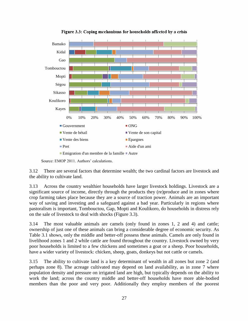
27
Source: EMOP 2011. Authors’ calculations.
3.12 There are several factors that determine wealth; the two cardinal factors are livestock and
the ability to cultivate land.
3.13 Across the country wealthier households have larger livestock holdings. Livestock are a
significant source of income, directly through the products they (re)produce and in zones where
crop farming takes place because they are a source of traction power. Animals are an important
way of saving and investing and a safeguard against a bad year. Particularly in regions where
pastoralism is important, Tombouctou, Gap, Mopti and Koulikoro, do households in distress rely
on the sale of livestock to deal with shocks (Figure 3.3).
3.14 The most valuable animals are camels (only found in zones 1, 2 and 4) and cattle;
ownership of just one of these animals can bring a considerable degree of economic security. As
Table 3.1 shows, only the middle and better-off possess these animals. Camels are only found in
livelihood zones 1 and 2 while cattle are found throughout the country. Livestock owned by very
poor households is limited to a few chickens and sometimes a goat or a sheep. Poor households,
have a wider variety of livestock: chicken, sheep, goats, donkeys but not cattle or camels.
3.15 The ability to cultivate land is a key determinant of wealth in all zones but zone 2 (and
perhaps zone 8). The acreage cultivated may depend on land availability, as in zone 7 where
population density and pressure on irrigated land are high, but typically depends on the ability to
work the land; across the country middle and better-off households have more able-bodied
members than the poor and very poor. Additionally they employ members of the poorest
0% 10% 20% 30% 40% 50% 60% 70% 80% 90% 100%
Kayes
Koulikoro
Sikasso
Ségou
Mopti
Tombouctou
Gao
Kidal
Bamako
Gouvernment ONG
Vente de bétail Vente de son capital
Vente des biens Epargnes
Pret Aide d'un ami
Emigration d'un membre de la famille Autre
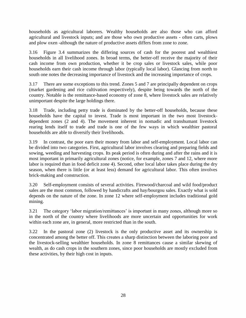
28
households as agricultural laborers. Wealthy households are also those who can afford
agricultural and livestock inputs; and are those who own productive assets - often carts, plows
and plow oxen -although the nature of productive assets differs from zone to zone.
3.16 Figure 3.4 summarizes the differing sources of cash for the poorest and wealthiest
households in all livelihood zones. In broad terms, the better-off receive the majority of their
cash income from own production, whether it be crop sales or livestock sales, while poor
households earn their cash income through labor (typically local labor). Glancing from north to
south one notes the decreasing importance of livestock and the increasing importance of crops.
3.17 There are some exceptions to this trend. Zones 5 and 7 are principally dependent on crops
(market gardening and rice cultivation respectively), despite being towards the north of the
country. Notable is the remittance-based economy of zone 8, where livestock sales are relatively
unimportant despite the large holdings there.
3.18 Trade, including petty trade is dominated by the better-off households, because these
households have the capital to invest. Trade is most important in the two most livestock-
dependent zones (2 and 4). The movement inherent in nomadic and transhumant livestock
rearing lends itself to trade and trade is one of the few ways in which wealthier pastoral
households are able to diversify their livelihoods.
3.19 In contrast, the poor earn their money from labor and self-employment. Local labor can
be divided into two categories. First, agricultural labor involves clearing and preparing fields and
sowing, weeding and harvesting crops. Its peak period is often during and after the rains and it is
most important in primarily agricultural zones (notice, for example, zones 7 and 12, where more
labor is required than in food deficit zone 4). Second, other local labor takes place during the dry
season, when there is little (or at least less) demand for agricultural labor. This often involves
brick-making and construction.
3.20 Self-employment consists of several activities. Firewood/charcoal and wild food/product
sales are the most common, followed by handicrafts and hay/bourgou sales. Exactly what is sold
depends on the nature of the zone. In zone 12 where self-employment includes traditional gold
mining.
3.21 The category ‘labor migration/remittances’ is important in many zones, although more so
in the north of the country where livelihoods are more uncertain and opportunities for work
within each zone are, in general, more restricted than in the south.
3.22 In the pastoral zone (2) livestock is the only productive asset and its ownership is
concentrated among the better off. This creates a sharp distinction between the laboring poor and
the livestock-selling wealthier households. In zone 8 remittances cause a similar skewing of
wealth, as do cash crops in the southern zones, since poor households are mostly excluded from
these activities, by their high cost in inputs.
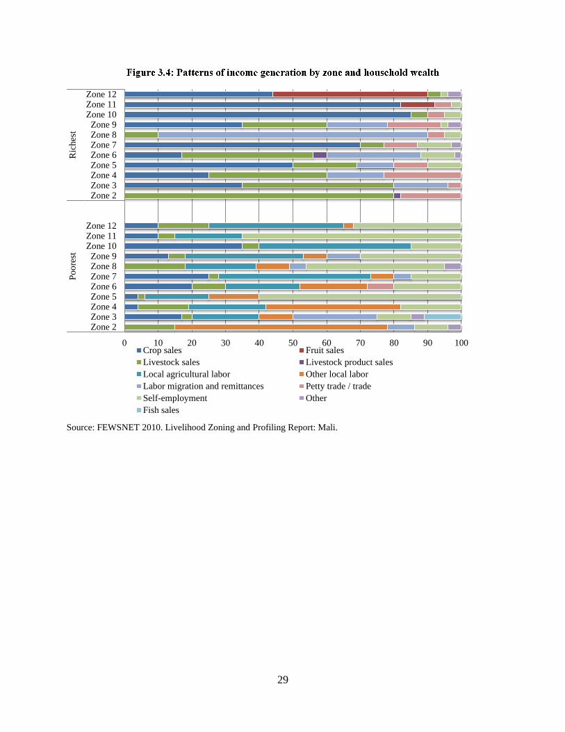
29
Source: FEWSNET 2010. Livelihood Zoning and Profiling Report: Mali.
0 10 20 30 40 50 60 70 80 90 100
Zone 2Zone 3Zone 4Zone 5Zone 6Zone 7Zone 8Zone 9
Zone 10Zone 11Zone 12
Zone 2Zone 3Zone 4Zone 5Zone 6Zone 7Zone 8Zone 9
Zone 10Zone 11Zone 12
Po
ore
stR
iches
t
Crop sales Fruit sales
Livestock sales Livestock product sales
Local agricultural labor Other local labor
Labor migration and remittances Petty trade / trade
Self-employment Other
Fish sales

30
Very poor
Per
cen
t
Ho
use
ho
l
d s
ize
La
nd
cult
iva
ted
Sh
eep
Go
ats
Do
nk
eys
Ca
mel
s
Ca
ttle
Plo
ug
h
Ox
en
Po
ult
ry
Other assets
2. Nomadic and transhumant pastoralism 30.0 6 - 0 0 1 0 0 0 0 4-6 small ruminants on loan from better off
3. Fluvial rice and transhumant livestock rearing 25.0 7 0.8 0 1 0 0 0 0 5 2-3 small ruminants on loan from better off
4. Millet and transhumant livestock rearing 15.0 3 0.3 0 0 0 0 0 0 5
5. Dogon plateau 15.0 4 0.5 0 0 0 0 0 0 5
6. Niger delta - rice and livestock rearing 10.0 4 1 0 0 0 0 0 0 4
7. Office du Niger (irrigated rice) 10.0 5 1 1 0 1 0 0 0 10
8. Remittances, sorghum, transhumant livestock 8.0 5 1 0 5 0 0 0 0 10
9. West and central rain-fed millet/sorghum 25.0 4 1 0 1 0 0 0 0 20
10. Sorghum, millet and cotton 15.0 4 2 0 0 0 0 0 0 2
11. South maize, cotton and fruits 10.0 4 2 0 0 0 0 0 0 10
12. South-west maize, sorghum and fruits 10.0 4 2 0 0 0 0 0 0 5
Poor
2. Nomadic and transhumant pastoralism 27.0 8 - 6 15 2 0 0 0 0 4-6 small ruminants on loaned from better off
3. Fluvial rice and transhumant livestock rearing 30.0 9 1.5 1 4 1 0 0 0 5 0-2 fishing nets; 2-3 small ruminants on loan
4. Millet and transhumant livestock rearing 40.0 10 1.0 1 4 0 0 0 0 8
5. Dogon plateau 43.0 10 3 2 1 1 0 0 0 10
6. Niger delta - rice and livestock rearing 40.0 7 2 4 7 2 0 0 0 12
7. Office du Niger (irrigated rice) 25.0 10 1 3 2 1 0 0 0 20 1 plow, 1 cart
8. Remittances, sorghum, transhumant livestock 25.0 12 2 2 10 2 0 0 0 20
9. West and central rain-fed millet/sorghum 30.0 8 3 2 4 1 0 1 0 30
10. Sorghum, millet and cotton 35.0 9 5 4 4 1 0 1 0 7 1 plow
11. South maize, cotton and fruits 20.0 10 5 0 5 0 0 0 0 30 1 plow
12. South-west maize, sorghum and fruits 30.0 6 4 0 2 0 0 0 0 10 1 plow

31
Middle
Per
cen
t
Ho
use
ho
l
d s
ize
La
nd
cult
iva
ted
Sh
eep
Go
ats
Do
nk
eys
Ca
mel
s
Ca
ttle
Plo
ug
h
Ox
en
Po
ult
ry
2. Nomadic and transhumant pastoralism 23.0 11 - 40 35 4 25 10 0 0
3. Fluvial rice and transhumant livestock rearing 25.0 11 5.5 8 13 2 0 9 2 6 0-1 canoe, 0-2 plows, 0-2 fishing nets
4. Millet and transhumant livestock rearing 35.0 20 4.0 7 20 2 1 22 0 18 1-2 carts, 1 plow
5. Dogon plateau 32.0 17 6 4 11 2 0 6 0 15 1-2 motorized pumps, 1 plow, 1 cart
6. Niger delta - rice and livestock rearing 35.0 11 7 10 15 2 0 25 0 25 1-2 plows, 1 cart
7. Office du Niger (irrigated rice) 50.0 20 4 7 5 2 0 6 0 20 2 plows, 1 cart
8. Remittances, sorghum, transhumant livestock 55.0 25 6 30 20 4 0 30 0 20 1-2 plows, 1 cart, 2-3 full time agricultural workers
9. West and central rain-fed millet/sorghum 40.0 12 8 10 10 2 0 6 0 40 1 plow, 1 cart, 1 seeding machine
10. Sorghum, millet and cotton 40.0 17 17 12 12 1 0 8 0 25 2 plows, 1 cart, 1 seeding machine, 1 motor cultivator
11. South maize, cotton and fruits 60.0 15 8 3 10 2 0 10 0 40
2 plows, 1 cart, 1 seeding machine, 1 motor cultivator, 2
fertilizer equipment
12. South-west maize, sorghum and fruits 50.0 10 11 6 8 2 0 10 0 30
1 plows, 1 cart, 1 seeding machine, 1 motor cultivator, 2
fertilizer equipment, orchards
Better off
2. Nomadic and transhumant pastoralism 20.0 18 - 70 35 8 50 25 0 0
3. Fluvial rice and transhumant livestock rearing 20.0 15 9.0 15 23 5 0 22 4
0-2 canoes, 1-2 plows, 0-2 fishing nets, 0-2 motor pumps
4. Millet and transhumant livestock rearing 10.0 35 8.0 17 40 4 2 35 0 25 3-4 carts, 2 plows
5. Dogon plateau 10.0 25 10 13 30 2 0 15 0 18 2-3 motorized pumps, 2-3 plow2, 2 carts
6. Niger delta - rice and livestock rearing 15.0 20 14 25 40 5 0 50 0 0 3-4 plows, 2-3 carts
7. Office du Niger (irrigated rice) 15.0 30 8 15 10 4 0 30 0 25 3-4 plows, 2-3 carts, 1 motorized cultivator
8. Remittances, sorghum, transhumant livestock 12.0 45 25 40 50 6 0 10
0 0 30 4-5 plows, 3-4 carts, 5-6 full time agricultural workers
9. West and central rain-fed millet/sorghum 5.0 20 15 30 30 4 0 30 0 60 2 plows, 2 carts, 1 seeding machine, 1 motorized cultivator,
2 full time agricultural laborers
10. Sorghum, millet and cotton 10.0 30 35 25 25 3 0 50 0 60 4 plows, 2 carts, 2 seeding machines, 2 motor cultivators
11. South maize, cotton and fruits 10.0 20 15 6 10 3 0 20 0 50 4 plows, 2 carts, 2 seeding machines, 2 motor cultivators, 2
fertilizer equipment
12. South-west maize, sorghum and fruits 10.0 15 20 10 8 3 0 35 0 60 4 plows, 2 carts, 2 seeding machines, 2 motor cultivators, 2
fertilizer equipment, orchards
Source: Calculated from FEWSNET 2010. Livelihood Zoning and Profiling Report: Mali.

32
3.23 Patterns of food consumption differ across livelihood zones and across wealth categories.
At the most general level, there is a north-south trend whereby households in the south depend
more on own production for food and less on the market. A difference exists between zones 3
and 4 in the north, which produce a deficit, import staple foods and are food insecure, and zones
10, 11 and 12 in the south, which produce a surplus, export cereals and are food secure.
However, households in all zones rely on the market for their food needs. Even in the south, the
very poor and poor depend heavily on the market and must use cash income to purchase food.
Thus the graph reveals something about the structure of poverty in that poor households are more
dependent on food purchases than are the better off households who mostly rely on own
production to meet their food needs.
Source: FEWSNET 2010. Livelihood Zoning and Profiling Report: Mali.
3.24 In all zones the poorest households receive payments in-kind for work carried out for the
middle and better-off. Under this type of arrangement wealthier households pay laborers using
grain from their own harvests; zone 2 is distinctive in that there is payment in-kind in bought
grain, but no agricultural production. In all zones the poor and very poor receive some of their
0 10 20 30 40 50 60 70 80 90 100
Zone 2
Zone 3
Zone 4
Zone 5
Zone 6
Zone 7
Zone 8
Zone 9
Zone 10
Zone 11
Zone 12
Zone 2
Zone 3
Zone 4
Zone 5
Zone 6
Zone 7
Zone 8
Zone 9
Zone 10
Zone 11
Zone 12
Po
ore
stR
iches
t
Own production Payment in kind Purchase
Loan and gift in kind Wild foods Labor migration
Milk an dlivestock products Other
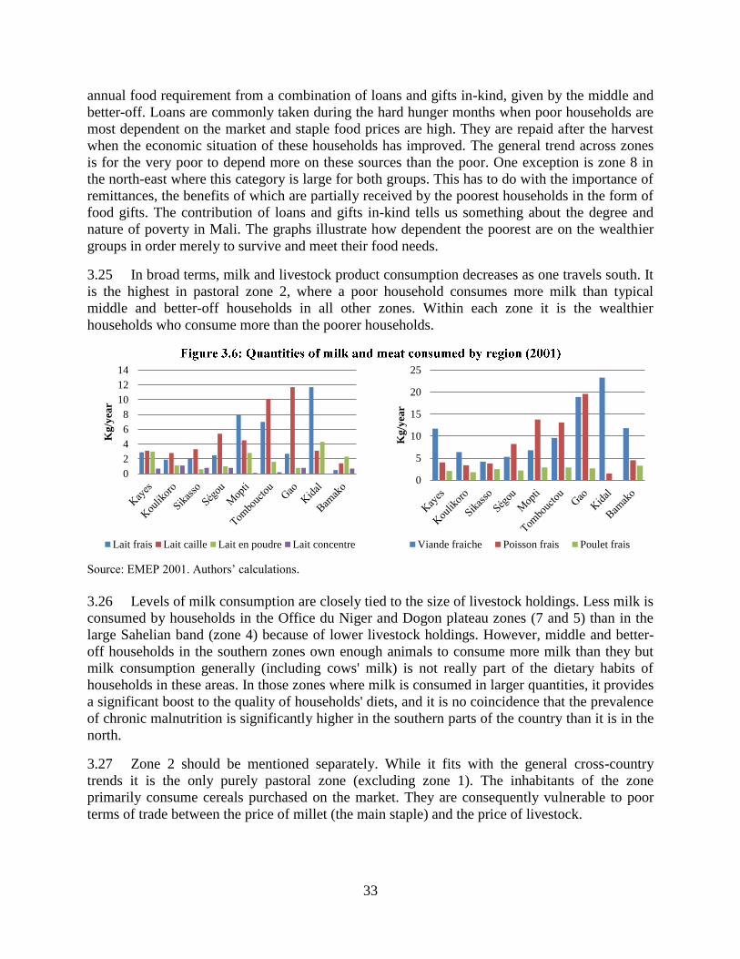
33
annual food requirement from a combination of loans and gifts in-kind, given by the middle and
better-off. Loans are commonly taken during the hard hunger months when poor households are
most dependent on the market and staple food prices are high. They are repaid after the harvest
when the economic situation of these households has improved. The general trend across zones
is for the very poor to depend more on these sources than the poor. One exception is zone 8 in
the north-east where this category is large for both groups. This has to do with the importance of
remittances, the benefits of which are partially received by the poorest households in the form of
food gifts. The contribution of loans and gifts in-kind tells us something about the degree and
nature of poverty in Mali. The graphs illustrate how dependent the poorest are on the wealthier
groups in order merely to survive and meet their food needs.
3.25 In broad terms, milk and livestock product consumption decreases as one travels south. It
is the highest in pastoral zone 2, where a poor household consumes more milk than typical
middle and better-off households in all other zones. Within each zone it is the wealthier
households who consume more than the poorer households.
Source: EMEP 2001. Authors’ calculations.
3.26 Levels of milk consumption are closely tied to the size of livestock holdings. Less milk is
consumed by households in the Office du Niger and Dogon plateau zones (7 and 5) than in the
large Sahelian band (zone 4) because of lower livestock holdings. However, middle and better-
off households in the southern zones own enough animals to consume more milk than they but
milk consumption generally (including cows' milk) is not really part of the dietary habits of
households in these areas. In those zones where milk is consumed in larger quantities, it provides
a significant boost to the quality of households' diets, and it is no coincidence that the prevalence
of chronic malnutrition is significantly higher in the southern parts of the country than it is in the
north.
3.27 Zone 2 should be mentioned separately. While it fits with the general cross-country
trends it is the only purely pastoral zone (excluding zone 1). The inhabitants of the zone
primarily consume cereals purchased on the market. They are consequently vulnerable to poor
terms of trade between the price of millet (the main staple) and the price of livestock.
0
2
4
6
8
10
12
14
Kg
/yea
r
Lait frais Lait caille Lait en poudre Lait concentre
0
5
10
15
20
25
Kg
/yea
r
Viande fraiche Poisson frais Poulet frais
34
3.28 Access to services differs across livelihood zones. The first aspect to note is that in
Bamako access to piped water, electricity as well as the use of (modern) toilet facilities is much
higher than elsewhere. At the same time the number of schools per ‘000 residents, as well as the
number of health facilities per ‘000 residents is amongst the lowest in the country. This pattern
has been observed before in Chapter 2: better access to piped water and electricity are associated
with high population density. The lower number of schools and health facilities is possibly also a
reflection of high density in that in a high density environment one can benefit from economies
of density and construct larger schools and health centers.
3.29 Between the different livelihood zones, access to piped water and electricity varies, but it
is in essence uniformly low, with the exception of households in zone 8 (Northern Kayes) who
rely on remittances amongst whom some 14 percent of households have access to electricity.
1 Nomadism and trans-Saharan trade Very poor.
2 Nomadic and transhumant pastoralism Sand and dirt roads are most frequent in this region, with very
few surfaced with bitumen. Market access in the zone is poor and
herders may have to travel long distances to take their animals to
market.
3 Fluvial rice and transhumant livestock
rearing (agropastoral)
Market access varies; communes in the middle section of the
zone are fairly isolated as the river flows along the edge of the
desert. During the rainy season, for example, it takes sometimes
two to three days to travel by road from Téméra to Gao.
4 Millet and transhumant livestock rearing Access to markets in this zone is generally easy during the dry
season, although areas of the zone are isolated. Access becomes
more difficult in the rainy season.
5 Dogon plateau -- millet, shallots, wild
foods and tourism
Market access is relatively good and better than in zone 6.
6 Niger delta - rice and livestock rearing
(agropastoral)
Market access in this zone is worse than in zones 4 and 5 and
during the flooding many roads are impassable. Trading is also
carried out by canoe and motorized canoes; this decreases from
March to July when the water levels are low.
7 Office du Niger (irrigated rice) Markets are generally accessible in all seasons, although during
the rains some areas can be cut off.
8 North-west remittances, sorghum and
transhumant livestock rearing
Access to markets is relatively poor; during the dry season roads
can very sandy and in the wet season very muddy.
9 West and central rainfed millet/sorghum Markets access in this zone is generally good; however, it can
become very difficult in some areas during the wet season,
because of rivers and muddy roads.
10 Sorghum, millet and cotton Market access is generally good, but can become difficult in
some areas during the rainy season.
11 South maize, cotton and fruits Market access is generally good, apart from during the rains
when areas can become isolated and lorries easily get bogged
down on the roads. Roads may also be blocked by seasonal
rivers.
12 South-west maize, sorghum and fruits Market access is this zone is generally good, but can become
difficult in some areas during the rainy season.
13 Bamako Good
Source: FEWSNET 2010. Authors’ compilation.

35
3.30 In the previous chapter it was noted that there is a clear pattern in the number of schools
or health centers, with relatively more schools and health facilities in low density areas
agglomerations (villages). Doing the breakdown by livelihood zone, one notes a substantial
variation which can only be partially explained. For instance, in the desert (zone 1) one finds a
relatively high number of schools, which is a reflection of the low population density
necessitating the construction of relatively many (presumably small) schools. But in Southern
Sikasso (zone 11) one finds a comparable number of schools, while in other low density areas
such as in zones 2 and 4 the number of schools per ‘000 residents seems pretty low. In chapter 5
we will consider the placement of schools across the country in greater detail.
3.31 Access to markets also varies by livelihood zone and is closely associated with
population density: it is worst in the north of the country (zones 1,2 and 3) better in the middle
(zones 4, 8 and 9) and best in the south (zones 10, 11 and 12).

36
Livelihood zone
Population
density
Households
whose main
supply of
water is from
a faucet
Households
whose main
supply of
water is
from a well
or bore hole
Households
with
electricity
Househo
lds with
toilets
Househol
ds using
latrines
Schools
(per '000
residents)
Health
centers
(per '000
residents)
1. Nomadism and trans-Saharan trade 0.2 2.5% 87.6% 0.6% 1.4% 15.8% 1.81 0.21
2. Nomadic and transhumant pastoralism 1.9 5.3% 73.2% 3.8% 2.5% 20.7% 0.77 0.23
3. Fluvial rice and transhumant livestock
rearing 27.3 1.0% 63.0% 0.5% 2.5% 40.0% 0.88 0.11
4. Millet and transhumant livestock
rearing 7.7 4.1% 77.1% 1.7% 4.3% 35.6% 0.57 0.05
5. Dogon plateau 44.5 2.5% 84.1% 3.4% 2.5% 15.4% 0.71 0.07
6. Niger delta - rice and livestock rearing 33.0 5.2% 72.4% 5.1% 5.1% 54.9% 0.39 0.06
7. Office du Niger (irrigated rice) 180.9 5.3% 85.9% 6.3% 8.4% 82.6% 0.84 0.05
8. Remittances, sorghum, transhumant
livestock 18.4 14.1% 71.3% 2.4% 7.2% 71.9% 0.80 0.13
9. West and central rain-fed
millet/sorghum 27.7 5.2% 83.0% 3.7% 7.1% 73.1% 0.90 0.10
10. Sorghum, millet and cotton 52.3 2.4% 92.0% 2.2% 5.4% 72.9% 0.89 0.12
11. South maize, cotton and fruits 33.7 3.2% 89.5% 4.1% 7.0% 79.4% 1.76 0.24
12. South-west maize, sorghum and fruits 19.2 2.2% 83.4% 3.0% 4.1% 65.1% 1.27 0.14
13. Bamako 7380.0 44.5% 27.9% 76.9% 21.5% 74.9% 0.54 0.09
Source: 2009 census of the Malian population. Authors’ calculations.

37
3.32 In the predominantly agricultural zones of Mali the ability to cultivate is the most
important determinant of wealth. In most livelihood zones access to land is not a limiting factor
but access to labor, to agricultural inputs and productive assets is.30
Hence a key difference
between wealthier and poorer households is less how much land they possess and more how
much land they are able to cultivate.
3.33 The number of able-bodied household members and the ownership of productive assets
(plow, oxen, fishing nets, motorized pumps) are critical determinants of the acreage that can be
cultivated and, consequently, of poverty. Poor households typically lack both and end-up with a
production system in which they cultivate small plots of land, obtain low yields and depend on
labor income to make ends meet. Once in it, it is very hard to escape this low productivity
system.
3.34 Poor households do not own the livestock to provide them with organic manure, nor do
they own carts (or the donkeys or the cattle to pull them) with which to transport manure to the
fields. Hence the poorest households do not use manure and are not able to fertilize their fields.
3.35 When the time for land preparation comes, access to a plow and plow oxen is important
as land preparation is labor-intensive. Poor households may own a plow, but will typically lack
the oxen. By the time oxen can be borrowed or rented, the better off households owning the
animals have already completed planting and the optimal time for planting has past. In the
meantime, poor households may prepare their land using the traditional daba (a type of hoe), thus
limiting the acreage that can be sowed. Alternatively they may opt (or be forced to) first work for
wealthier households, before devoting themselves to their own fields. In either case, poor
households sow late, weed less, and consequently receive lower yields.
3.36 Since little land is brought under cultivation, poor households prefer to grow food crops
over cash crops like cotton: these are predominantly grown by the better off households. It means
poor households forego the possibility to access fertilizer on credit which is offered by the
CDMT. So in comparison to better-off households, poor households not only have less able-
bodied household members, they end up working for better off households as laborers, are
unable to afford agricultural inputs such as fertilizer and pesticides, and do not grow cash crops
such as cotton.
3.37 The food poor household obtain from their own plots is insufficient to sustain them till
the next harvest (in fact some of it may be eaten prematurely prior to the harvest–thus reducing
yields further) and poor households rely heavily on casual labor as a source of income and on
markets to purchase their food. The dependence on food and labor markets may seem at odds
with the perception of poor households being subsistence households. The subsistence aspect
only references to the fact that poor households interact little with the market as a producer. As a
net purchaser of food, and as an active participant in the labor market, access to markets is
critical to poor households. Market access varies, however, across the county and is worst in the
north and in the west (Figure 3.7). In chapter 5 we will note that limited market access, is in turn
associated to high levels of consumption variability.
30
About 3.2 million hectares out of a total of 12 million with cultivation potential is cultivated.
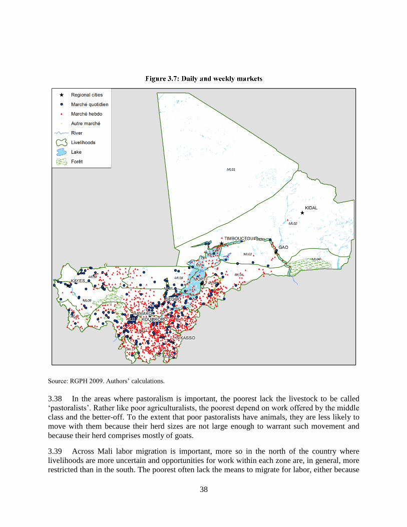
38
Source: RGPH 2009. Authors’ calculations.
3.38 In the areas where pastoralism is important, the poorest lack the livestock to be called
‘pastoralists’. Rather like poor agriculturalists, the poorest depend on work offered by the middle
class and the better-off. To the extent that poor pastoralists have animals, they are less likely to
move with them because their herd sizes are not large enough to warrant such movement and
because their herd comprises mostly of goats.
3.39 Across Mali labor migration is important, more so in the north of the country where
livelihoods are more uncertain and opportunities for work within each zone are, in general, more
restricted than in the south. The poorest often lack the means to migrate for labor, either because

39
they have too few able-bodied members or lack the cash to pay for transport. Hence the very
poor look for casual labor opportunities nearby, and often end up doing tasks like weeding,
plowing, winnowing, harvesting and construction work. Other kinds of work include
shepherding, fishing and punting/paddling canoes.
3.40 If poor households do migrate they tend to migrate less far than better off households
who have the means to pay for travel over long distances. Poor household thus have to forego the
most remunerative sources of income open to the better of who may end up working in Ghana,
Mauretania, Côte d’Ivoire, Algeria or even in Europe.
3.41 To diversify their income base, poor households may seek to self-employ by collecting
and sell firewood and wild fruits or by producing charcoal. Again the options open to the poor
are limited as they lack the capital to engage in more remunerative self-employment options such
as trade, commerce or agricultural transformation.
3.42 The dependence on labor as their main asset makes poor households extremely
vulnerable to health shocks. Malaria is a particularly important acute source of risk. When
malaria strikes during the lean season when food stocks have run out and households depend on
the income able bodied household members are able to make, or during the planting season when
the presence of able bodied household members determines the size of next years’ harvest, the
consequences can be severe. Malnutrition is a more chronic type of risk: high levels of anemia
(in part caused by frequent bouts of malaria and regular infections) reduce labor productivity,
and poor diets (poor households do not drink milk) increase the risk of stunting.
3.43 Dependence on purchased food during the lean season make poor households rely more
on wild foods (which are labor intensive to collect) and exposes poor households to the vagaries
of the market. Rising food prices and falling livestock prices are particularly harmful to the
poorest; for pastoralists the worst possible combination is one of falling livestock prices and
rising food prices, a combination that typically occurs when a covariate shock (drought, insects,
insecurity) affects an area.
3.44 The need for able bodied people to work also means that children from very poor
households are more likely to receive only a basic primary education (if at all), thus given an
intergenerational dimension to poverty.
3.45 The 13 livelihood zones offer a rich description of the various ways production systems
in the country. By delving deeper into the ways people earn a living it has become clear that poor
households are not able to realize their full productive potential. Policies that allow poor
households to break the cycle of poverty seem critical. As land is still relatively abundant, such
policies should seek ways to increase the capital base of poor households and/or to increase their
labor productivity. Policies leading to greater access to traction animals, improved seed or
fertilizer seem critical as do policies that reduce exposure to malaria and anemia and policies that
offer labor opportunities during the lean season.

40

41
Source: SMART 2013.
3.46 Poor households are (surprisingly?) dependent on food and labor markets. Low food
prices –often seen as critical for the urban poor, are equally critically for poor people in rural
areas. Increasing food production would be pro-poor as it can be expected to increase the
demand for labor and to reduce food prices. In the next section we will see that, indeed,
livelihood zones where poverty has dropped the fastest are those where food production has
increased.
3.47 Poor households are found not to have much livestock –even in pastoralist zones, and are
less likely to be involved in transhumant livestock rearing – other than as herders. Hence policies
that increase the demand for their labor may be more astute to reducing poverty than
interventions aimed at cattle or other large animals; also interventions that focus on small
ruminants can be expected to benefit non-poor households disproportionately.
3.48 The dependence on able-bodied household members for their labor is likely to exert a
negative influence on children from poor households to go to school, and particularly to
secondary school as the opportunity cost to labor is rises with age. Indeed for every 100 children
from the poorest wealth quintile attending primary school, only 36 continue to secondary school;
for children from the top wealth quintile the corresponding number is 57. Policies that reduce the
opportunity cost to labor while increasing school attendance would be welcome. This could
include reducing the age at school entry, but also offering school meals
31
34
38 39 40 38
36
15
24 25
29
24 22 23
2 2 3 2 2
1 2
0
5
10
15
20
25
30
35
40
45
Bamako Kayes Koulikoro Mopti Ségou Sikasso Mali
Per
cen
t
Anémie Légère Anémie Modérée Anémie Sévère

42
Explaining Well-being Using a Spatial Perspective
4.1 Well-being has different dimensions from happiness to poverty and from life expectancy
to literacy. In this chapter the focus is on those elements of well-being that are largely
determined at the household level, while aspects determined by decisions of the state are
discussed in the next chapter. Hence we discuss life expectancy, mortality and nutrition but not
access to health care. We consider literacy, but not access to education. We primarily focus on
consumption, ownership of assets as well as income poverty. In the next chapter we deal with
access to services.
4.2 The perspective remains a spatial one. We combine information about the livelihood zone
with household surveys and explore how poverty and poverty trends vary spatially and what
might explain these trends. We also consider more typical correlates of welfare such as education
and nutrition. At times the relation may be as expected: better educated people have, on average,
higher levels of consumption and lower levels of poverty. In other instances, the relation is less
obvious such as the relation between acute malnutrition and average levels of consumption.
4.3 Consumption captures the ability of an individual to meet his or her basic and other
needs. In doing so it is an important metric of well-being. Consumption data can be obtained
from household surveys. For Mali three comparable nationwide household surveys are available.
These surveys were administrated in 2001 (EMEP), 2006 (ELIM) and in 2009/2010 (ELIM) 31
and had sample sizes of 4966, 4494 and 9235 households respectively. The surveys had modules
capturing information about household consumption as well as dwelling characteristics, durable
goods ownership, education etc. The consumption measure we use is defined as the aggregate of
all household consumption, expressed in 2001 prices. This aggregate includes cash expenditure
on food and non-food items, consumption of home produced goods, and user values of owned
durable goods. A provision for owner-occupied dwellings is also taken into account.
4.4 Two other household surveys, EMOP32
, were implemented in 2011 and 2013. Unlike the
three annual surveys carried out between 2001 and 2010, the EMOP surveys are quarterly. The
consumption information they collect, however, is not comparable to that collected earlier.
Hence we treat this information separately. For 2013 only information for the first two waves is
available. As we are interested in trends most of our analysis will focus on data collected
between 2001 and 2010.
4.5 In 2010, levels of consumption in rural areas were approximately half (FCFA 119,000
per capita) those in urban areas (FCFA 239,000 per capita). Price differences between rural and
31
The 2001 survey was the Enquête Malienne d’Évaluation de la Pauvreté (EMEP), the Enquête Légère Intégrée
auprès des Ménages (ELIM) in 2006 and the Enquête par grappes à Indicateurs Multiples et de dépenses des
ménages (MICS-ELIM) in 2009 /2010. 32
Enquête Modulaire et Permanente auprès des Ménages (EMOP).

43
urban areas – life in urban areas is more expensive than in rural areas,33
reduce the difference in
real terms but it is evident that levels of consumption are considerably higher in urban than in
rural areas. Because of the large differences in consumption, the poorest households – those in
the first two wealth quintiles are almost exclusively found in the rural areas, whereas the richest
households are almost exclusively found in urban areas (Figure 4.1). Out of approximately 1
million rural households, only 90,000 belong to the top wealth quintile, while of the
approximately 330,000 urban households, more than half belong to the top wealth quintile.
Source: ELIM 2010. Authors’ calculations.
4.6 Breaking down the data by region one finds that expressed in consumption per capita,
households in Sikasso are worst off and those in Bamako best off (Figure 4.2). By expressing
consumption in per capita terms, we do not take into account that households in Sikasso are
amongst the largest, nor that not all household members have equal consumption needs, or that
certain consumption items (such as televisions or radios) can be shared. One approach to take
these aspects into consideration is by defining the number of adult equivalents. This can be done
using a formula where A is the number of adults in the household, and K is the number of
children. The parameter α is the cost of a child relative to that of an adult, and lies somewhere
between 0 and 1. The other parameter, β also lies between 0 and 1 and controls the extent of
economies of scale.
Adult equivalent = (A + αK) β
When both a and β are unity—the most extreme case—the number of adult equivalents is simply
household size, and consumption is expressed on a per capita basis.
4.7 Values for a used by INSTAT are provided in the footnote.34
The values suggest that
children are relatively cheap: small children count for less than half an adult. If we think of
33
This is reflected in the urban poverty lines which are approximately 20 percent higher than those for rural areas. 34
In Mali the following adult equivalence scales are used.
12,624 21,867 44,881
87,160
176,953
254,124 244,914 221,731
179,573
89,719
-
50,000
100,000
150,000
200,000
250,000
300,000
Le plus pauvre 2 3 4 Le plus riche
Quintile de consommation
Nu
mb
er o
f h
ou
seh
old
s
urbain rural

44
economies of scale as coming from the existence of shared goods in the household, then β has to
be high since households in Mali spend a large fraction of their budget on food and relatively
little on shared public goods. Deaton and Zaidi (2002) suggest to set in such circumstances the
economies of scale factor to 0.9.35
Source: ELIM 2010. Authors’ calculations.
4.8 Figure 4.2 presents the results for consumption per adult equivalent under various
assumptions. The first panel presents consumption per capita (setting α to 1 for all household
members); the second panel presents consumption per adult equivalent. The third panel does the
same but accounts for economies of scale at the household level as well (setting β equal to 0.9).
The Figure demonstrates that irrespective of the assumptions made the patterns of consumption
do not differ: those living in Sikasso invariably consume least, closely followed by those in
Ségou and Mopti while those living in Kayes, Kidal and particularly in Bamako consume most.
Because of the insensitivity of the pattern of consumption to the choice of adult equivalent
measure, we use per capita consumption in the remainder of this document.
4.9 Consumption data can also be presented by livelihood zone (see Figure 4.3). It is
informative in that – in addition to the large difference with Bamako, it demonstrates that
average consumption in two livelihoods zones, 4 (millet and transhumant livestock keeping) and
10 (sorghum, millet and cotton) are particularly low, while two other livelihood zones 2
Age range Male Female Age range Male Female
0-1 0.26 0.26 15-18 1.03 0.76
1-3 0.45 0.45 19-24 1 0.76
4-6 0.62 0.62 25-50 1 0.76
7-10 0.69 0.69 51-99 0.79 0.66
11-14 0.86 0.76
35
Deaton, A. and S. Zaidi (2002). A Guide to Aggregating Consumption Expenditures, Living Standards
Measurement Study, Working Paper 135.
172
128 104 111 117
140 148
218
279 239
176 143 152 162
194 205
300
367
298
220 179 189 196
230 245
348
449
0
50
100
150
200
250
300
350
400
450
500
Kay
es
Ko
uli
koro
Sik
asso
Ség
ou
Mo
pti
To
mb
ouct
ou
Gao
Kid
al
Bam
ako
Kay
es
Ko
uli
koro
Sik
asso
Ség
ou
Mo
pti
To
mb
ouct
ou
Gao
Kid
al
Bam
ako
Kay
es
Ko
uli
koro
Sik
asso
Ség
ou
Mo
pti
To
mb
ouct
ou
Gao
Kid
al
Bam
ako
Consommation par habitant Consommation par equivalent
adulte
Consommation par equivalent
adulte (avec facteur d'echelle)
Co
nsu
mp
tio
n (
FC
FA
'0
00
)
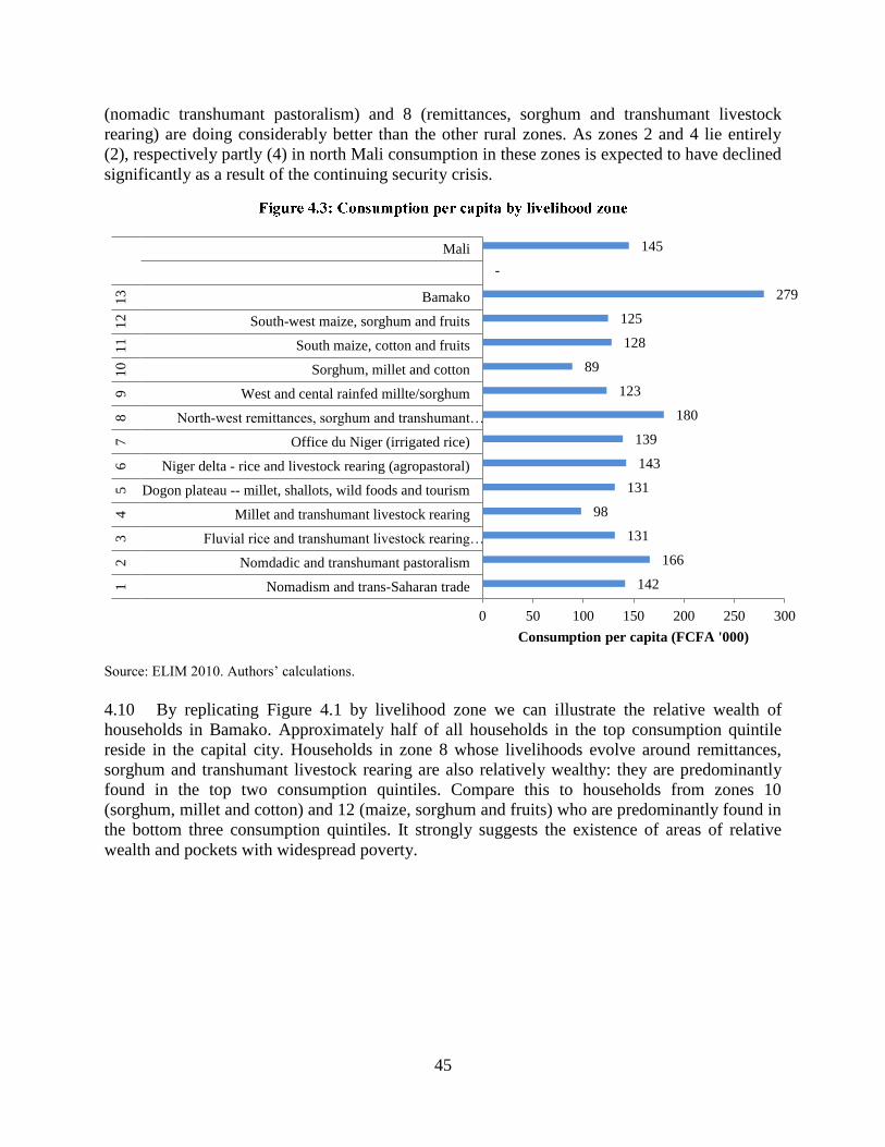
45
(nomadic transhumant pastoralism) and 8 (remittances, sorghum and transhumant livestock
rearing) are doing considerably better than the other rural zones. As zones 2 and 4 lie entirely
(2), respectively partly (4) in north Mali consumption in these zones is expected to have declined
significantly as a result of the continuing security crisis.
Source: ELIM 2010. Authors’ calculations.
4.10 By replicating Figure 4.1 by livelihood zone we can illustrate the relative wealth of
households in Bamako. Approximately half of all households in the top consumption quintile
reside in the capital city. Households in zone 8 whose livelihoods evolve around remittances,
sorghum and transhumant livestock rearing are also relatively wealthy: they are predominantly
found in the top two consumption quintiles. Compare this to households from zones 10
(sorghum, millet and cotton) and 12 (maize, sorghum and fruits) who are predominantly found in
the bottom three consumption quintiles. It strongly suggests the existence of areas of relative
wealth and pockets with widespread poverty.
142
166
131
98
131
143
139
180
123
89
128
125
279
-
145
0 50 100 150 200 250 300
Nomadism and trans-Saharan trade
Nomdadic and transhumant pastoralism
Fluvial rice and transhumant livestock rearing…
Millet and transhumant livestock rearing
Dogon plateau -- millet, shallots, wild foods and tourism
Niger delta - rice and livestock rearing (agropastoral)
Office du Niger (irrigated rice)
North-west remittances, sorghum and transhumant…
West and cental rainfed millte/sorghum
Sorghum, millet and cotton
South maize, cotton and fruits
South-west maize, sorghum and fruits
Bamako
Mali
12
34
56
78
91
01
11
21
3
Consumption per capita (FCFA '000)

46
Source: ELIM 2010. Authors’ calculations.
4.11 Based on the 2001 EMEP survey poverty lines were constructed by a joint
INSTAT/World Bank team following the cost of basic needs approach.36
To this end food
poverty lines were computed for each of the nine regions by identifying and costing the food
baskets consumed by Malian households that provide 2450 kcal per capita per day. That food
basket included some 20 items representing around 80% of the total food expenditure. The
quantities in this basket were then scaled so that they would provide exactly 2450 kilocalories
per day. The non-food component of the poverty line was estimated using the non-food
expenditure level of the households whose food consumption was within five percent of the food
poverty line. The poverty lines were estimated for rural and urban areas within each region
except Bamako which is exclusively urban.
4.12 One of the drawbacks of the approach used is that the non-food poverty lines were based
on a very small number of observations. For example the urban non-food poverty line for Kayes
used the non-food expenditure of 14 households. For Sikasso 14 respectively 53 observations
were used for urban and rural areas. The most extreme case was Gao where only four urban and
nine rural observations were used.
4.13 A consequence of estimating non-food poverty lines using such a small number of
observations is the considerable variation in the size of the non-food share components across
regions. This is illustrated in Figure 4.5: in rural and urban Sikasso but also in urban Ségou are
the non-food components very large relative to their comparators. Such large non-food
36
See Backiny-Yetna et al. (2007).
-
50,000
100,000
150,000
200,000
250,000
300,000
Le plus
pauvre
2 3 4 Le plus
riche
Quintile de consommation
Nu
mb
er o
f h
ou
seh
old
s
13. Bamako
12. South-west maize, sorghum and
fruits11. South maize, cotton and fruits
10. Sorghum, millet and cotton
9. West and central rainfed
millet/sorghum8. Remittances, sorghum,
transhumant livestock rearing7. Office du Niger (irrigated rice)
6. Niger delta - rice and livestock
rearing5. Dogon plateau -- millet, shallots,
wild foods, tourism4. Millet and transhumant livestock
rearing3. Fluvial rice and transhumant
livestock rearing2. Nomadic and transhumant
pastoralism
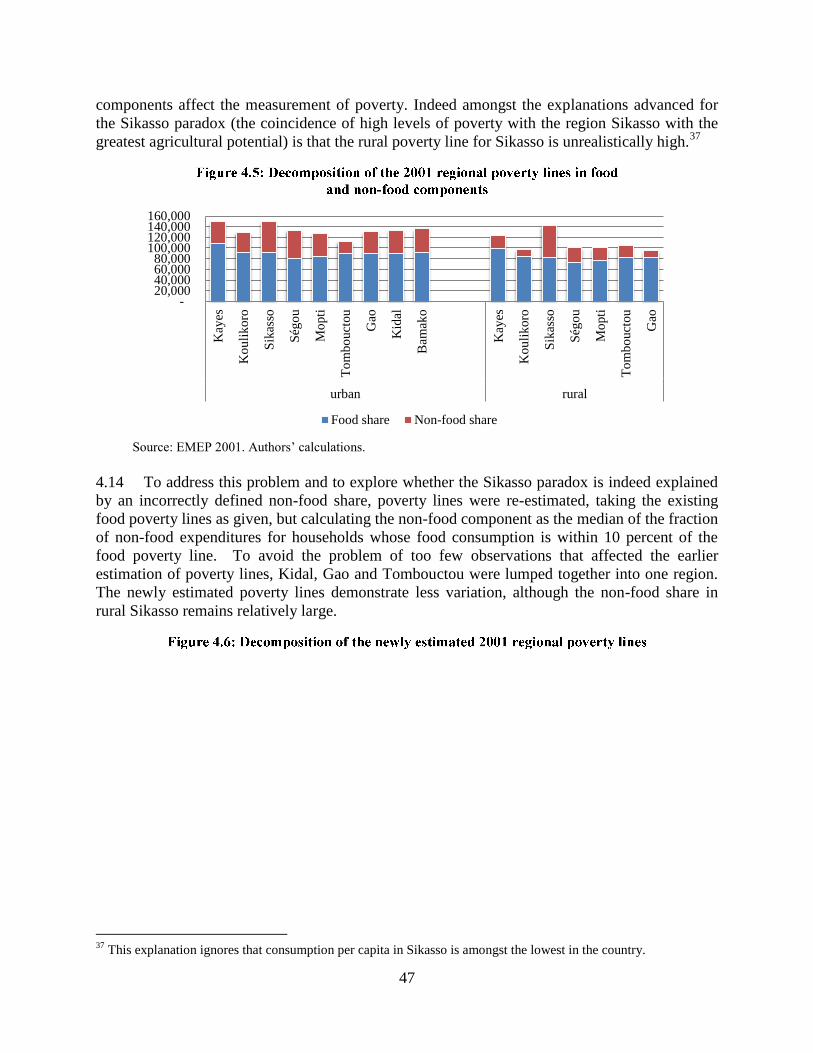
47
components affect the measurement of poverty. Indeed amongst the explanations advanced for
the Sikasso paradox (the coincidence of high levels of poverty with the region Sikasso with the
greatest agricultural potential) is that the rural poverty line for Sikasso is unrealistically high.37
Source: EMEP 2001. Authors’ calculations.
4.14 To address this problem and to explore whether the Sikasso paradox is indeed explained
by an incorrectly defined non-food share, poverty lines were re-estimated, taking the existing
food poverty lines as given, but calculating the non-food component as the median of the fraction
of non-food expenditures for households whose food consumption is within 10 percent of the
food poverty line. To avoid the problem of too few observations that affected the earlier
estimation of poverty lines, Kidal, Gao and Tombouctou were lumped together into one region.
The newly estimated poverty lines demonstrate less variation, although the non-food share in
rural Sikasso remains relatively large.
37
This explanation ignores that consumption per capita in Sikasso is amongst the lowest in the country.
- 20,000 40,000 60,000 80,000
100,000 120,000 140,000 160,000
Kay
es
Ko
uli
koro
Sik
asso
Ség
ou
Mo
pti
To
mb
ouct
ou
Gao
Kid
al
Bam
ako
Kay
es
Ko
uli
koro
Sik
asso
Ség
ou
Mo
pti
To
mb
ouct
ou
Gao
urban rural
Food share Non-food share
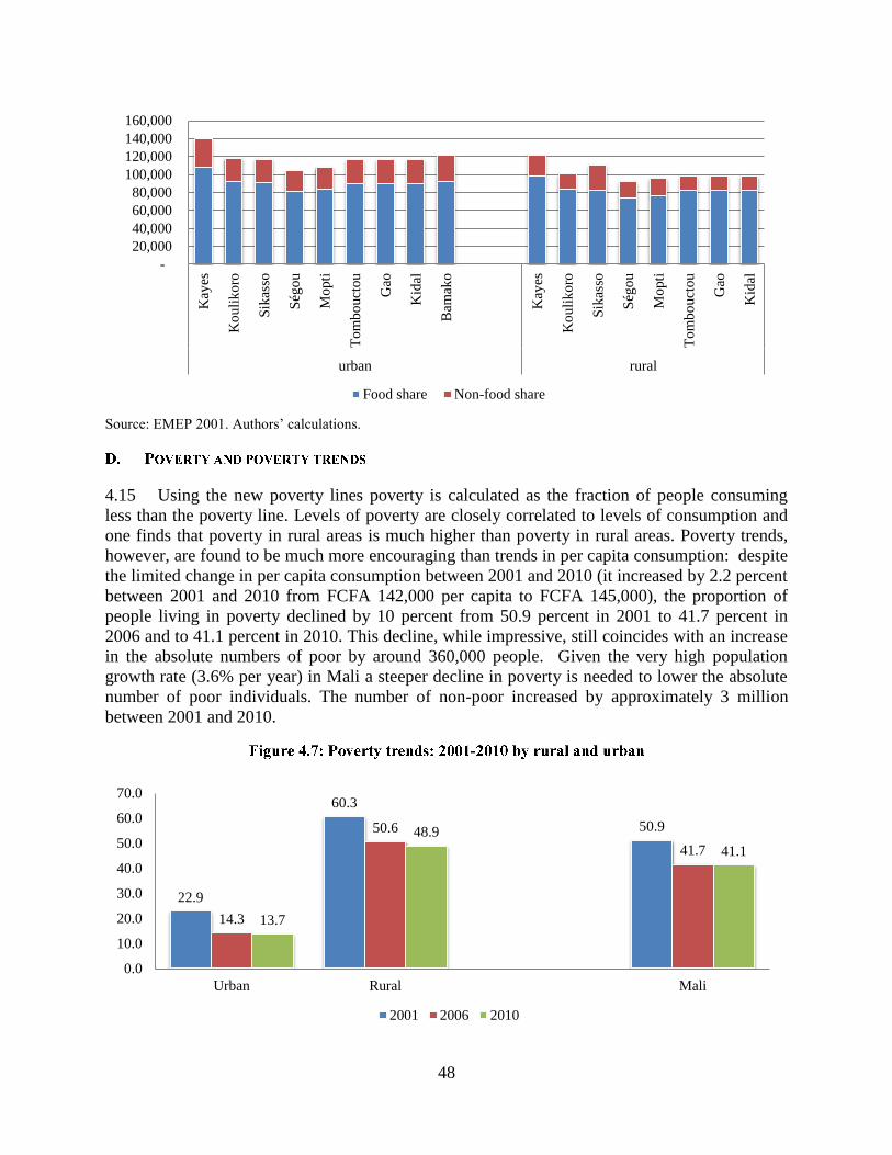
48
Source: EMEP 2001. Authors’ calculations.
4.15 Using the new poverty lines poverty is calculated as the fraction of people consuming
less than the poverty line. Levels of poverty are closely correlated to levels of consumption and
one finds that poverty in rural areas is much higher than poverty in rural areas. Poverty trends,
however, are found to be much more encouraging than trends in per capita consumption: despite
the limited change in per capita consumption between 2001 and 2010 (it increased by 2.2 percent
between 2001 and 2010 from FCFA 142,000 per capita to FCFA 145,000), the proportion of
people living in poverty declined by 10 percent from 50.9 percent in 2001 to 41.7 percent in
2006 and to 41.1 percent in 2010. This decline, while impressive, still coincides with an increase
in the absolute numbers of poor by around 360,000 people. Given the very high population
growth rate (3.6% per year) in Mali a steeper decline in poverty is needed to lower the absolute
number of poor individuals. The number of non-poor increased by approximately 3 million
between 2001 and 2010.
-
20,000
40,000
60,000
80,000
100,000
120,000
140,000
160,000
Kay
es
Ko
uli
koro
Sik
asso
Ség
ou
Mo
pti
To
mb
ouct
ou
Gao
Kid
al
Bam
ako
Kay
es
Ko
uli
koro
Sik
asso
Ség
ou
Mo
pti
To
mb
ouct
ou
Gao
Kid
al
urban rural
Food share Non-food share
22.9
60.3
50.9
14.3
50.6
41.7
13.7
48.9
41.1
0.0
10.0
20.0
30.0
40.0
50.0
60.0
70.0
Urban Rural Mali
2001 2006 2010

49
4.16 Most of the decline in poverty was realized between 2001 and 2006, while between 2006
and 2010 very little changed. The rapid reduction in poverty is explained by the fact that for the
poorest households consumption grew most rapidly, while for the better off households
consumption grew much more slowly: in fact for households in the top wealth quintile
consumption fell between 2001 and 2010. This is illustrated in Figure 4.8, presenting growth
incidence curves for the period 2001-2010, and curves for the sub-periods 2001-2006 and 2006-
2010. The Figure covering the entire period demonstrates that consumption growth was positive
for households up to the 78th
percentile (the curve lies above the zero line) and growth was
highest for the poorest households. Consequently growth was pro-poor – even though the
average per capita rate of growth was very low (only 0.2% per annum), consumption was being
redistributed towards the poor. It is therefore unsurprising that the reduction in poverty coincided
with a fall in the Gini coefficient from 0.40 in 2001 to 0.33 in 2010.
4.17 The curves for the sub-periods 2001-2006 and 2006-2010 demonstrate that the patterns of
growth were very different for each sub-period. During the first half of the decade growth was
positive for households in all wealth categories, with households in the 2nd
and 3rd
decile
benefiting most. In the second half of the decade, between 2006 and 2010, growth continued to
be positive for the poorest households, but for households in the 3rd
till the 7th
decile it was
negligible, while for the wealthiest households it was negative. Figure 4.8: Growth incidence
curve national level: 2001-2010
-4
-2
0
2
4
6
8
0 3 6 9 12 15 18 21 24 27 30 33 36 39 42 45 48 51 54 57 60 63 66 69 72 75 78 81 84 87 90 93 96 99
An
nu
al
gro
wth
ra
te, %
Expenditure percentiles
2001-2010

50
Source: EMEP 2001, ELIM 2006 and ELIM 2010. Authors’ calculations.
4.18 Considering changes in poverty from a regional perspective one notes how poverty
declined rapidly in Kayes, Koulikoro and Mopti. In Koulikoro and Mopti most of the decline
occurred during the first half of the decade, in Kayes the reduction in poverty continued
throughout the period. The reduction in poverty in these two regions, contrasts with that in
Sikasso where poverty remained very high and largely unchanged. In Ségou, Tombouctou and
Gao, finally, regions with the lowest incidence of poverty (apart from Kidal and Bamako which
have even lower poverty levels), levels of poverty increased somewhat.
-2
-1
0
1
2
3
4
5
6
7
0 10 20 30 40 50 60 70 80 90 100
An
nu
al
gro
wth
ra
te, %
Expenditure percentiles
2001-2006
-15
-10
-5
0
5
10
15
0 10 20 30 40 50 60 70 80 90 100
An
nu
al
gro
wth
ra
te, %
Expenditure percentiles
2006-2010
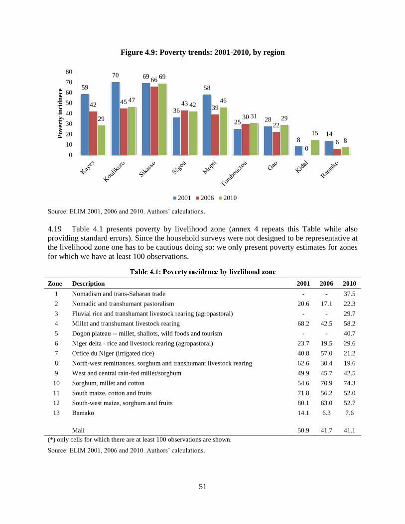
51
Figure 4.9: Poverty trends: 2001-2010, by region
Source: ELIM 2001, 2006 and 2010. Authors’ calculations.
4.19 Table 4.1 presents poverty by livelihood zone (annex 4 repeats this Table while also
providing standard errors). Since the household surveys were not designed to be representative at
the livelihood zone one has to be cautious doing so: we only present poverty estimates for zones
for which we have at least 100 observations.
Zone Description 2001 2006 2010
1 Nomadism and trans-Saharan trade - - 37.5
2 Nomadic and transhumant pastoralism 20.6 17.1 22.3
3 Fluvial rice and transhumant livestock rearing (agropastoral) - - 29.7
4 Millet and transhumant livestock rearing 68.2 42.5 58.2
5 Dogon plateau -- millet, shallots, wild foods and tourism - - 40.7
6 Niger delta - rice and livestock rearing (agropastoral) 23.7 19.5 29.6
7 Office du Niger (irrigated rice) 40.8 57.0 21.2
8 North-west remittances, sorghum and transhumant livestock rearing 62.6 30.4 19.6
9 West and central rain-fed millet/sorghum 49.9 45.7 42.5
10 Sorghum, millet and cotton 54.6 70.9 74.3
11 South maize, cotton and fruits 71.8 56.2 52.0
12 South-west maize, sorghum and fruits 80.1 63.0 52.7
13 Bamako 14.1 6.3 7.6
Mali 50.9 41.7 41.1
(*) only cells for which there are at least 100 observations are shown.
Source: ELIM 2001, 2006 and 2010. Authors’ calculations.
59
70 69
36
58
25 28
8 14
42 45
66
43 39
30
22
0 6
29
47
69
42 46
31 29
15
8
0
10
20
30
40
50
60
70
80
Po
ver
ty i
nci
dn
ece
2001 2006 2010
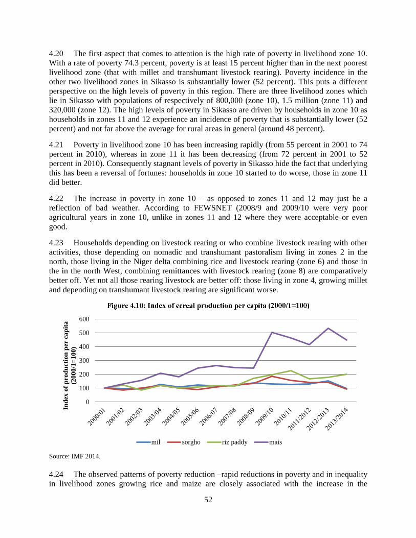
52
4.20 The first aspect that comes to attention is the high rate of poverty in livelihood zone 10.
With a rate of poverty 74.3 percent, poverty is at least 15 percent higher than in the next poorest
livelihood zone (that with millet and transhumant livestock rearing). Poverty incidence in the
other two livelihood zones in Sikasso is substantially lower (52 percent). This puts a different
perspective on the high levels of poverty in this region. There are three livelihood zones which
lie in Sikasso with populations of respectively of 800,000 (zone 10), 1.5 million (zone 11) and
320,000 (zone 12). The high levels of poverty in Sikasso are driven by households in zone 10 as
households in zones 11 and 12 experience an incidence of poverty that is substantially lower (52
percent) and not far above the average for rural areas in general (around 48 percent).
4.21 Poverty in livelihood zone 10 has been increasing rapidly (from 55 percent in 2001 to 74
percent in 2010), whereas in zone 11 it has been decreasing (from 72 percent in 2001 to 52
percent in 2010). Consequently stagnant levels of poverty in Sikasso hide the fact that underlying
this has been a reversal of fortunes: households in zone 10 started to do worse, those in zone 11
did better.
4.22 The increase in poverty in zone 10 – as opposed to zones 11 and 12 may just be a
reflection of bad weather. According to FEWSNET (2008/9 and 2009/10 were very poor
agricultural years in zone 10, unlike in zones 11 and 12 where they were acceptable or even
good.
4.23 Households depending on livestock rearing or who combine livestock rearing with other
activities, those depending on nomadic and transhumant pastoralism living in zones 2 in the
north, those living in the Niger delta combining rice and livestock rearing (zone 6) and those in
the in the north West, combining remittances with livestock rearing (zone 8) are comparatively
better off. Yet not all those rearing livestock are better off: those living in zone 4, growing millet
and depending on transhumant livestock rearing are significant worse.
Source: IMF 2014.
4.24 The observed patterns of poverty reduction –rapid reductions in poverty and in inequality
in livelihood zones growing rice and maize are closely associated with the increase in the
0
100
200
300
400
500
600
Ind
ex o
f p
rod
uct
ion
per
ca
pit
a
(20
00
/1=
10
0)
mil sorgho riz paddy mais

53
production of cereals. The remarkable increase is illustrated in Figure 4.10 presenting production
per capita. Production is expressed as an index to illustrate for the four most important cereal
crops, maize, rice, millet and sorghum the increase in production relative to the base year. Since
2000/1 maize production increased five-fold; particularly since 2008/9 one observes accelerating
maize production. The rapid increase in maize production is associated to the rapid decline in
poverty incidence in livelihoods zones 11 and 12, where most of the maize is grown. And, as the
growth incidence curves for zones 11 and 12 demonstrate, the increase in maize production has
been highly pro-poor. Poor households benefited even more from the boom in maize production
than did better of households. This comes as no surprise. For poor households who rely, in part,
on farm jobs for their income and who purchase much of their food needs, increased maize
production affects their welfare positively through at least two channels. Increasing cereal
production leads to more demand for farm work and secondly, increased cereal production
exercises downward pressure on (rural) food prices.38
Better off households also benefit from
increased cereal production but as net sellers of maize the positive effect of increased production
is mitigated by lower prices.
4.25 Like maize, rice production per capita increased significantly, doubling relative to
2001/1. The increase in rice production is equally reflected in the poverty trends: poverty in rice
growing areas declined, especially in the zone office du Niger and the areas where rice is grown
on the borders of the Niger around Tombouctou and Gao. As the growth incidence curve
demonstrates, and as was the case for maize, poor households benefited most from the increase
in rice production. It is somewhat surprising that households living in the Niger delta (zone 6)
have not been able to benefit from increased rice production. It will be explored later whether
this may be associated to a limited access to markets in the delta.
Source: IMF 2014.
38
A third channel is that poor households themselves increased their production and became less deficient in food.
-
20.00
40.00
60.00
80.00
100.00
120.00
140.00
160.00
180.00
200.00
-
100,000
200,000
300,000
400,000
500,000
600,000
700,000
va
lue
of
pro
du
ctio
n (
$ m
illi
on
s)
Pro
du
ctio
n (
ton
s)
Production (CMDT) Valuer de la production
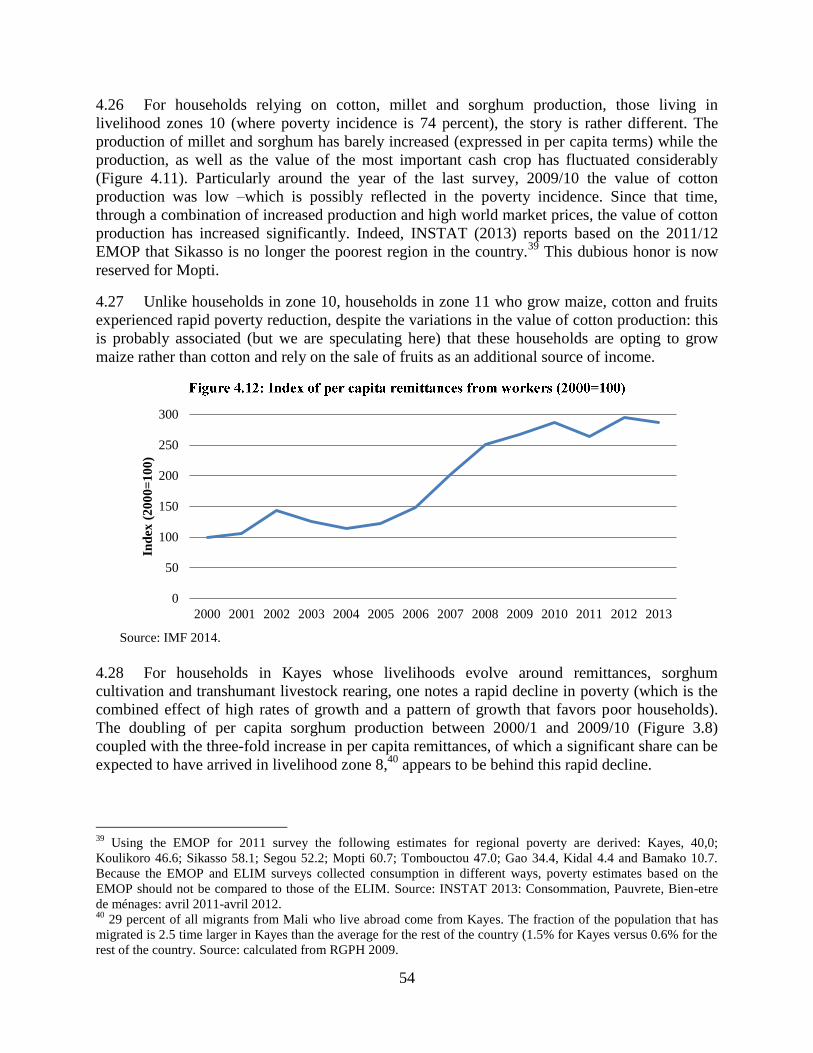
54
4.26 For households relying on cotton, millet and sorghum production, those living in
livelihood zones 10 (where poverty incidence is 74 percent), the story is rather different. The
production of millet and sorghum has barely increased (expressed in per capita terms) while the
production, as well as the value of the most important cash crop has fluctuated considerably
(Figure 4.11). Particularly around the year of the last survey, 2009/10 the value of cotton
production was low –which is possibly reflected in the poverty incidence. Since that time,
through a combination of increased production and high world market prices, the value of cotton
production has increased significantly. Indeed, INSTAT (2013) reports based on the 2011/12
EMOP that Sikasso is no longer the poorest region in the country.39
This dubious honor is now
reserved for Mopti.
4.27 Unlike households in zone 10, households in zone 11 who grow maize, cotton and fruits
experienced rapid poverty reduction, despite the variations in the value of cotton production: this
is probably associated (but we are speculating here) that these households are opting to grow
maize rather than cotton and rely on the sale of fruits as an additional source of income.
Source: IMF 2014.
4.28 For households in Kayes whose livelihoods evolve around remittances, sorghum
cultivation and transhumant livestock rearing, one notes a rapid decline in poverty (which is the
combined effect of high rates of growth and a pattern of growth that favors poor households).
The doubling of per capita sorghum production between 2000/1 and 2009/10 (Figure 3.8)
coupled with the three-fold increase in per capita remittances, of which a significant share can be
expected to have arrived in livelihood zone 8,40
appears to be behind this rapid decline.
39
Using the EMOP for 2011 survey the following estimates for regional poverty are derived: Kayes, 40,0;
Koulikoro 46.6; Sikasso 58.1; Segou 52.2; Mopti 60.7; Tombouctou 47.0; Gao 34.4, Kidal 4.4 and Bamako 10.7.
Because the EMOP and ELIM surveys collected consumption in different ways, poverty estimates based on the
EMOP should not be compared to those of the ELIM. Source: INSTAT 2013: Consommation, Pauvrete, Bien-etre
de ménages: avril 2011-avril 2012. 40
29 percent of all migrants from Mali who live abroad come from Kayes. The fraction of the population that has
migrated is 2.5 time larger in Kayes than the average for the rest of the country (1.5% for Kayes versus 0.6% for the
rest of the country. Source: calculated from RGPH 2009.
0
50
100
150
200
250
300
2000 2001 2002 2003 2004 2005 2006 2007 2008 2009 2010 2011 2012 2013
Ind
ex (
20
00
=1
00
)
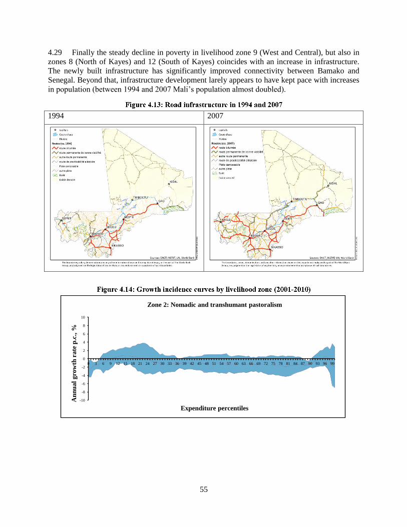
55
4.29 Finally the steady decline in poverty in livelihood zone 9 (West and Central), but also in
zones 8 (North of Kayes) and 12 (South of Kayes) coincides with an increase in infrastructure.
The newly built infrastructure has significantly improved connectivity between Bamako and
Senegal. Beyond that, infrastructure development larely appears to have kept pace with increases
in population (between 1994 and 2007 Mali’s population almost doubled).
1994 2007
-10
-8
-6
-4
-2
0
2
4
6
8
10
0 3 6 9 12 15 18 21 24 27 30 33 36 39 42 45 48 51 54 57 60 63 66 69 72 75 78 81 84 87 90 93 96 99
An
nu
al
gro
wth
ra
te p
.c.,
%
Expenditure percentiles
Zone 2: Nomadic and transhumant pastoralism
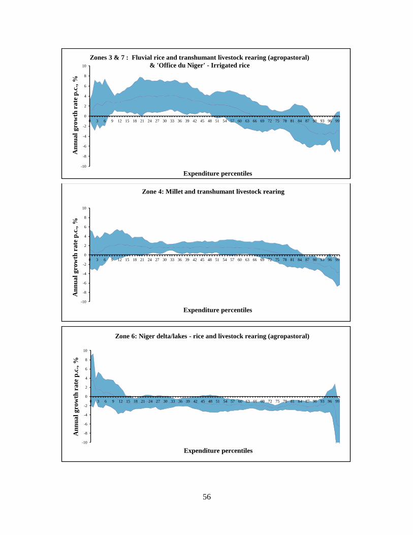
56
-10
-8
-6
-4
-2
0
2
4
6
8
10
0 3 6 9 12 15 18 21 24 27 30 33 36 39 42 45 48 51 54 57 60 63 66 69 72 75 78 81 84 87 90 93 96 99
An
nu
al
gro
wth
ra
te p
.c.,
%
Expenditure percentiles
Zones 3 & 7 : Fluvial rice and transhumant livestock rearing (agropastoral)
& 'Office du Niger' - Irrigated rice
-10
-8
-6
-4
-2
0
2
4
6
8
10
0 3 6 9 12 15 18 21 24 27 30 33 36 39 42 45 48 51 54 57 60 63 66 69 72 75 78 81 84 87 90 93 96 99
An
nu
al
gro
wth
ra
te p
.c.,
%
Expenditure percentiles
Zone 4: Millet and transhumant livestock rearing
-10
-8
-6
-4
-2
0
2
4
6
8
10
0 3 6 9 12 15 18 21 24 27 30 33 36 39 42 45 48 51 54 57 60 63 66 69 72 75 78 81 84 87 90 93 96 99
An
nu
al
gro
wth
ra
te p
.c.,
%
Expenditure percentiles
Zone 6: Niger delta/lakes - rice and livestock rearing (agropastoral)

57
-10
-8
-6
-4
-2
0
2
4
6
8
10
0 3 6 9 12 15 18 21 24 27 30 33 36 39 42 45 48 51 54 57 60 63 66 69 72 75 78 81 84 87 90 93 96 99
An
nu
al
gro
wth
ra
te p
.c.,
%
Expenditure percentiles
Zone 8: North-west remittances, sorghum, and transhumant livestock rearing
-10
-8
-6
-4
-2
0
2
4
6
8
10
0 3 6 9 12 15 18 21 24 27 30 33 36 39 42 45 48 51 54 57 60 63 66 69 72 75 78 81 84 87 90 93 96 99
An
nu
al
gro
wth
ra
te p
.c.,
%
Expenditure percentiles
Zone 9: West and central rainfed millet/sorghum
-10
-8
-6
-4
-2
0
2
4
6
8
10
0 3 6 9 12 15 18 21 24 27 30 33 36 39 42 45 48 51 54 57 60 63 66 69 72 75 78 81 84 87 90 93 96 99
An
nu
al
gro
wth
ra
te p
.c.,
%
Expenditure percentiles
Zone 10: Sorghum, millet, and cotton

58
Source: EMEP 2001 and ELIM 2010. Authors’ calculations.
4.30 Figure 4.16 presents the distribution of poor people across livelihood zones. One key
message from the Figure is that 70 percent of all poor are located in only three livelihood zones:
9 (west and central rain-fed millet/sorghum), 10 (sorghum, millet and cotton) and 11 (south,
maize, cotton and fruits). Encouraging is the fact that in the zone in which the greatest number of
poor can be found (zone 11) poverty has been falling, while the potential for further declines in
poverty seems real given the realistic prospect that the cotton and maize markets will continue to
expand and the fact that access to markets is relatively good (see chapter 5). Also in zone 9 (west
and central rain-fed millet/sorghum) poverty has been on the decline, albeit at a lower pace than
in zone 11. The zone that is in need of the greatest attention is zone 10, where 15% of poor
people reside and where poverty is on the increase. Zone 4 (millet and transhumant livestock
rearing) also needs to be mentioned, not only because some 10 percent of all poor live in this
zone, but also because it is not evident that much progress in poverty reduction is being made.
Poverty in this livelihood zone declined rapidly between 2001 and 2006 and then rose again in
2010. It can be expected that after 2010 poverty has increased further, due to the exposure of
households in this zone to the negative consequences of the conflict in the North.
-10
-8
-6
-4
-2
0
2
4
6
8
10
0 3 6 9 12 15 18 21 24 27 30 33 36 39 42 45 48 51 54 57 60 63 66 69 72 75 78 81 84 87 90 93 96 99
An
nu
al
gro
wth
ra
te p
.c.,
%
Expenditure percentiles
Zone 11: South maize, cotton, and fruits
-10
-8
-6
-4
-2
0
2
4
6
8
10
0 10 20 30 40 50 60 70 80 90 100
An
nu
al
gro
wth
ra
te, %
Expenditure percentiles
Zone 12: South-west maize, sorghum and fruits
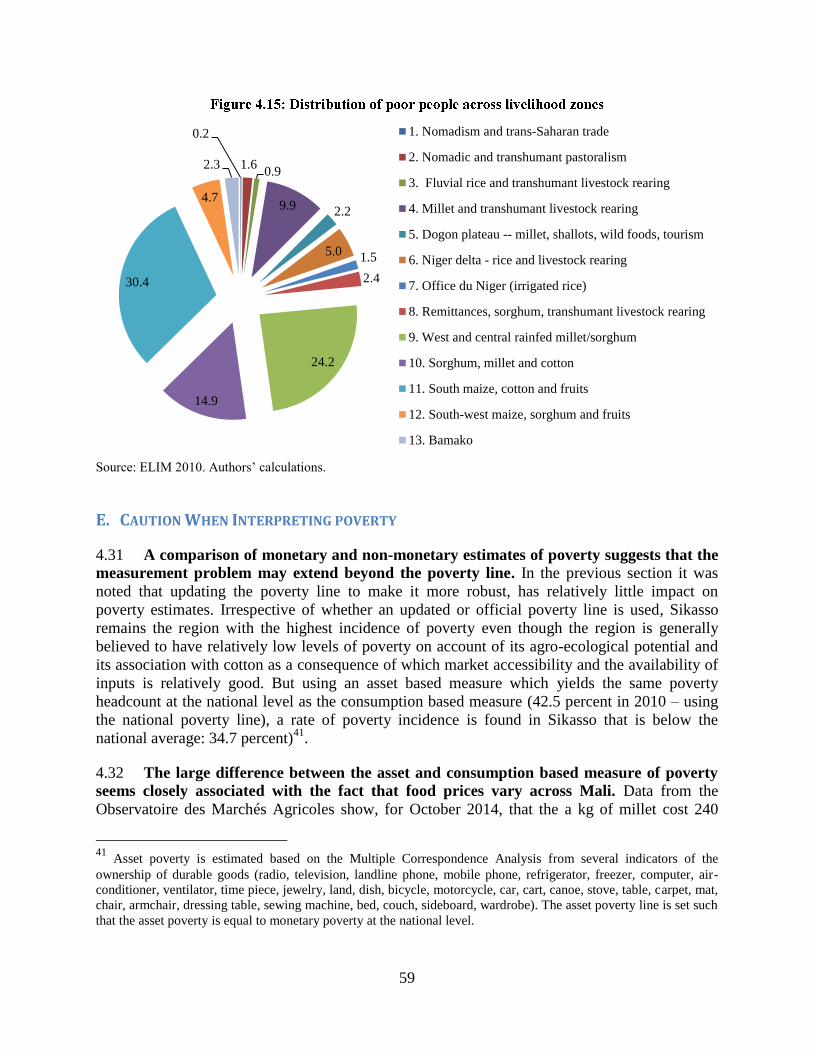
59
Source: ELIM 2010. Authors’ calculations.
E. CAUTION WHEN INTERPRETING POVERTY
4.31 A comparison of monetary and non-monetary estimates of poverty suggests that the
measurement problem may extend beyond the poverty line. In the previous section it was
noted that updating the poverty line to make it more robust, has relatively little impact on
poverty estimates. Irrespective of whether an updated or official poverty line is used, Sikasso
remains the region with the highest incidence of poverty even though the region is generally
believed to have relatively low levels of poverty on account of its agro-ecological potential and
its association with cotton as a consequence of which market accessibility and the availability of
inputs is relatively good. But using an asset based measure which yields the same poverty
headcount at the national level as the consumption based measure (42.5 percent in 2010 – using
the national poverty line), a rate of poverty incidence is found in Sikasso that is below the
national average: 34.7 percent)41
.
4.32 The large difference between the asset and consumption based measure of poverty
seems closely associated with the fact that food prices vary across Mali. Data from the
Observatoire des Marchés Agricoles show, for October 2014, that the a kg of millet cost 240
41
Asset poverty is estimated based on the Multiple Correspondence Analysis from several indicators of the
ownership of durable goods (radio, television, landline phone, mobile phone, refrigerator, freezer, computer, air-
conditioner, ventilator, time piece, jewelry, land, dish, bicycle, motorcycle, car, cart, canoe, stove, table, carpet, mat,
chair, armchair, dressing table, sewing machine, bed, couch, sideboard, wardrobe). The asset poverty line is set such
that the asset poverty is equal to monetary poverty at the national level.
0.2
1.6 0.9
9.9 2.2
5.0 1.5
2.4
24.2
14.9
30.4
4.7
2.3
1. Nomadism and trans-Saharan trade
2. Nomadic and transhumant pastoralism
3. Fluvial rice and transhumant livestock rearing
4. Millet and transhumant livestock rearing
5. Dogon plateau -- millet, shallots, wild foods, tourism
6. Niger delta - rice and livestock rearing
7. Office du Niger (irrigated rice)
8. Remittances, sorghum, transhumant livestock rearing
9. West and central rainfed millet/sorghum
10. Sorghum, millet and cotton
11. South maize, cotton and fruits
12. South-west maize, sorghum and fruits
13. Bamako
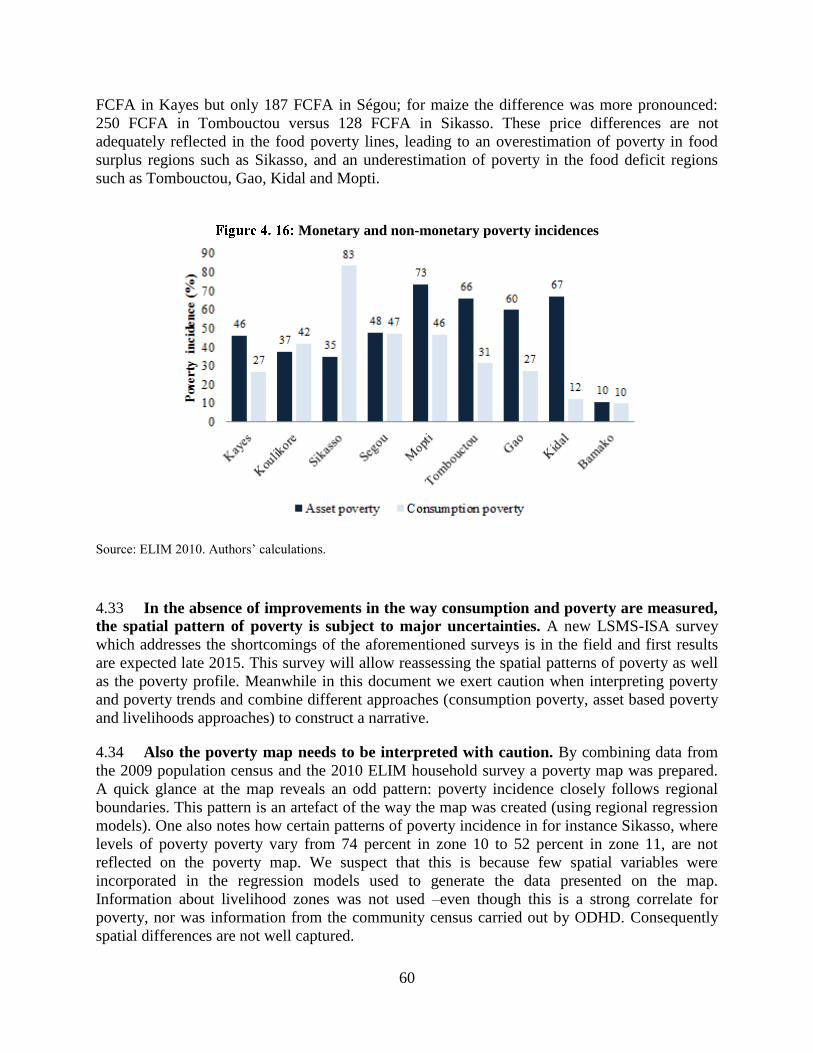
60
FCFA in Kayes but only 187 FCFA in Ségou; for maize the difference was more pronounced:
250 FCFA in Tombouctou versus 128 FCFA in Sikasso. These price differences are not
adequately reflected in the food poverty lines, leading to an overestimation of poverty in food
surplus regions such as Sikasso, and an underestimation of poverty in the food deficit regions
such as Tombouctou, Gao, Kidal and Mopti.
Monetary and non-monetary poverty incidences
Source: ELIM 2010. Authors’ calculations.
4.33 In the absence of improvements in the way consumption and poverty are measured,
the spatial pattern of poverty is subject to major uncertainties. A new LSMS-ISA survey
which addresses the shortcomings of the aforementioned surveys is in the field and first results
are expected late 2015. This survey will allow reassessing the spatial patterns of poverty as well
as the poverty profile. Meanwhile in this document we exert caution when interpreting poverty
and poverty trends and combine different approaches (consumption poverty, asset based poverty
and livelihoods approaches) to construct a narrative.
4.34 Also the poverty map needs to be interpreted with caution. By combining data from
the 2009 population census and the 2010 ELIM household survey a poverty map was prepared.
A quick glance at the map reveals an odd pattern: poverty incidence closely follows regional
boundaries. This pattern is an artefact of the way the map was created (using regional regression
models). One also notes how certain patterns of poverty incidence in for instance Sikasso, where
levels of poverty poverty vary from 74 percent in zone 10 to 52 percent in zone 11, are not
reflected on the poverty map. We suspect that this is because few spatial variables were
incorporated in the regression models used to generate the data presented on the map.
Information about livelihood zones was not used –even though this is a strong correlate for
poverty, nor was information from the community census carried out by ODHD. Consequently
spatial differences are not well captured.
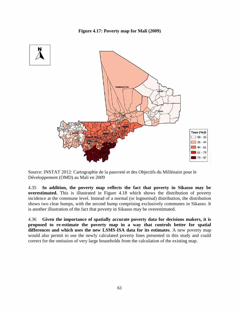
61
Figure 4.17: Poverty map for Mali (2009)
Source: INSTAT 2012: Cartographie de la pauvreté et des Objectifs du Millénaire pour le
Développement (OMD) au Mali en 2009
4.35 In addition, the poverty map reflects the fact that poverty in Sikasso may be
overestimated. This is illustrated in Figure 4.18 which shows the distribution of poverty
incidence at the commune level. Instead of a normal (or lognormal) distribution, the distribution
shows two clear humps, with the second hump comprising exclusively communes in Sikasso. It
is another illustration of the fact that poverty in Sikasso may be overestimated.
4.36 Given the importance of spatially accurate poverty data for decisions makers, it is
proposed to re-estimate the poverty map in a way that controls better for spatial
differences and which uses the new LSMS-ISA data for its estimates. A new poverty map
would also permit to use the newly calculated poverty lines presented in this study and could
correct for the omission of very large households from the calculation of the existing map.

62
Figure 4.18: Density estimate of poverty incidence at commune level
Source: Staff calculations based on 2009 poverty map
4.37 The EMOP surveys can be used to explore what happened to consumption after 2010.
The consumption aggregates derived from EMOP and ELIM are not comparable, so we only
present a comparison between the two EMOP surveys. To ensure comparability we express the
EMOP 2013 consumption in prices for 2011 (between the two surveys the rate of inflation was
6.0 percent, we only use waves 1 and 2 of both surveys (for EMOP 2013 preliminary data for the
two waves are available) and we exclude the regions of the North (they were not covered by
EMOP 2013 for reasons of security).
4.38 The data suggest that consumption declined significantly between 2011 and 2013: by 10
percent. This decline in consumption is unequally distributed. Consumption declined by as much
as 22 and 20 percent per capita in respectively Koulikoro and Mopti, declined by between 7 and
11 percent in Kayes, Ségou and Sikasso and increased in Bamako. These dramatic changes in
consumption are the combined effect of declines in the production of cereals as a result of bad
rains, an increase in the value of cotton production (see Figures 4.10 and 4.11) and spillovers
from the security crisis in North Mali.
0
.01
.02
.03
Den
sity
0 20 40 60 80 100Incidence of poverty (%)
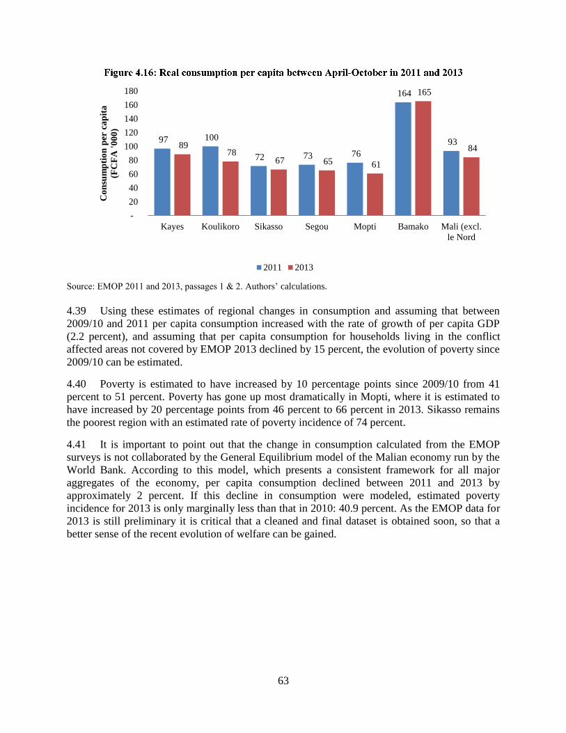
63
Source: EMOP 2011 and 2013, passages 1 & 2. Authors’ calculations.
4.39 Using these estimates of regional changes in consumption and assuming that between
2009/10 and 2011 per capita consumption increased with the rate of growth of per capita GDP
(2.2 percent), and assuming that per capita consumption for households living in the conflict
affected areas not covered by EMOP 2013 declined by 15 percent, the evolution of poverty since
2009/10 can be estimated.
4.40 Poverty is estimated to have increased by 10 percentage points since 2009/10 from 41
percent to 51 percent. Poverty has gone up most dramatically in Mopti, where it is estimated to
have increased by 20 percentage points from 46 percent to 66 percent in 2013. Sikasso remains
the poorest region with an estimated rate of poverty incidence of 74 percent.
4.41 It is important to point out that the change in consumption calculated from the EMOP
surveys is not collaborated by the General Equilibrium model of the Malian economy run by the
World Bank. According to this model, which presents a consistent framework for all major
aggregates of the economy, per capita consumption declined between 2011 and 2013 by
approximately 2 percent. If this decline in consumption were modeled, estimated poverty
incidence for 2013 is only marginally less than that in 2010: 40.9 percent. As the EMOP data for
2013 is still preliminary it is critical that a cleaned and final dataset is obtained soon, so that a
better sense of the recent evolution of welfare can be gained.
97 100
72 73 76
164
93 89 78
67 65 61
165
84
-
20
40
60
80
100
120
140
160
180
Kayes Koulikoro Sikasso Segou Mopti Bamako Mali (excl.
le Nord
Co
nsu
mp
tio
n p
er c
ap
ita
(FC
FA
'0
00
)
2011 2013
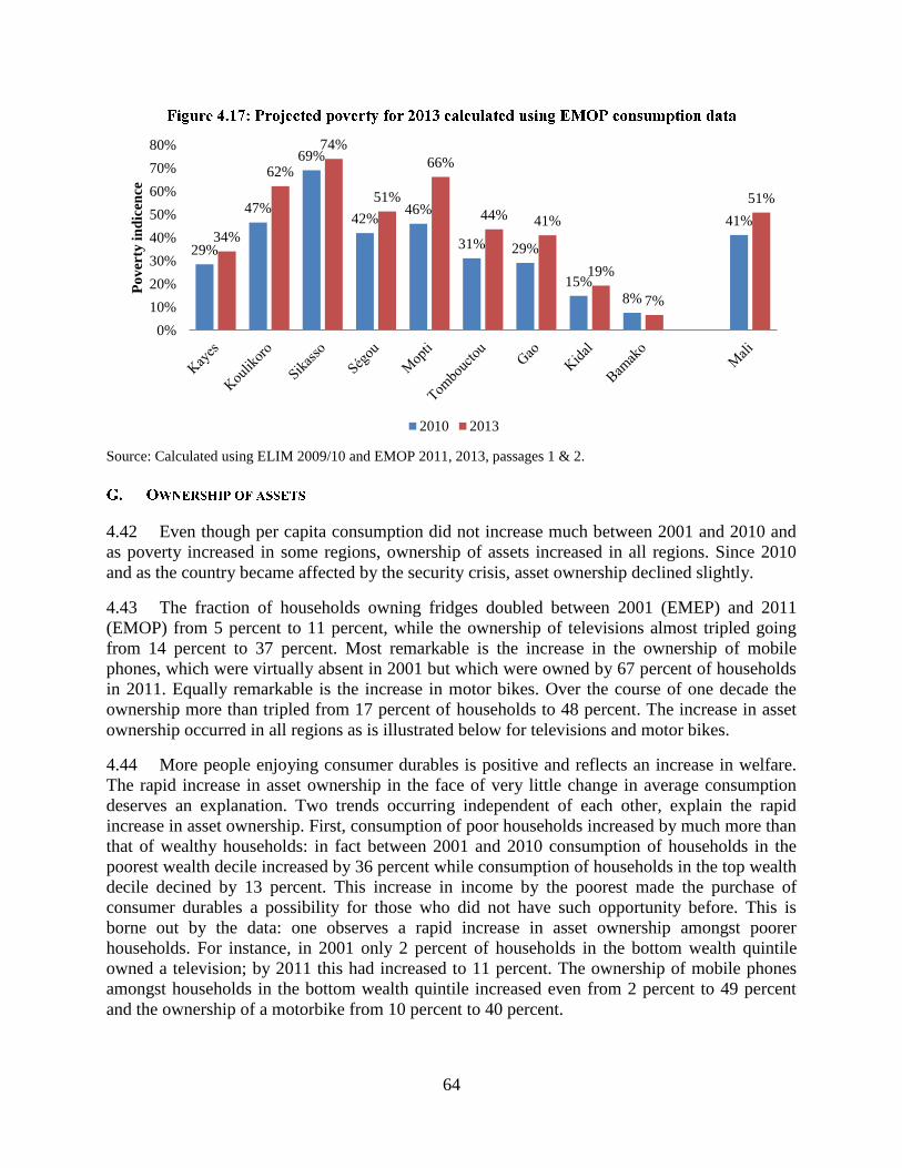
64
Source: Calculated using ELIM 2009/10 and EMOP 2011, 2013, passages 1 & 2.
4.42 Even though per capita consumption did not increase much between 2001 and 2010 and
as poverty increased in some regions, ownership of assets increased in all regions. Since 2010
and as the country became affected by the security crisis, asset ownership declined slightly.
4.43 The fraction of households owning fridges doubled between 2001 (EMEP) and 2011
(EMOP) from 5 percent to 11 percent, while the ownership of televisions almost tripled going
from 14 percent to 37 percent. Most remarkable is the increase in the ownership of mobile
phones, which were virtually absent in 2001 but which were owned by 67 percent of households
in 2011. Equally remarkable is the increase in motor bikes. Over the course of one decade the
ownership more than tripled from 17 percent of households to 48 percent. The increase in asset
ownership occurred in all regions as is illustrated below for televisions and motor bikes.
4.44 More people enjoying consumer durables is positive and reflects an increase in welfare.
The rapid increase in asset ownership in the face of very little change in average consumption
deserves an explanation. Two trends occurring independent of each other, explain the rapid
increase in asset ownership. First, consumption of poor households increased by much more than
that of wealthy households: in fact between 2001 and 2010 consumption of households in the
poorest wealth decile increased by 36 percent while consumption of households in the top wealth
decile decined by 13 percent. This increase in income by the poorest made the purchase of
consumer durables a possibility for those who did not have such opportunity before. This is
borne out by the data: one observes a rapid increase in asset ownership amongst poorer
households. For instance, in 2001 only 2 percent of households in the bottom wealth quintile
owned a television; by 2011 this had increased to 11 percent. The ownership of mobile phones
amongst households in the bottom wealth quintile increased even from 2 percent to 49 percent
and the ownership of a motorbike from 10 percent to 40 percent.
29%
47%
69%
42% 46%
31% 29%
15%
8%
41% 34%
62%
74%
51%
66%
44% 41%
19%
7%
51%
0%
10%
20%
30%
40%
50%
60%
70%
80%P
ov
erty
in
dic
ence
2010 2013

65
Televisions Motor bikes
Percent owning
Unit cost
Source: Asset data (ELIM and EMOP), price data (Mercuriales 2005-2012).
4.45 The second trend is that consumer durables became more affordable because prices
dropped. Since the early 2000s East-Asian manufacturers have begun to flood the market with
cheap consumer durables. Price data collected and published in the Mercuriale demonstrate how
the nominal price of a 21 inch televisions dropped from FCFA 180,000 to 110,000 a 40 percent
drop in nominal terms and an almost 50 percent drop if inflation is taken into account. The
pattern for motor bikes is slightly different. Here the price of the premium brand from Japan did
not drop much (in nominal terms at least), but the arrival of alternatives –they are first recorded
in the Mercuriale in 2005, the power KTM and a Yamaha from China, meant that households
now could purchase a motor bike which cost less than a third of the price of the Japanese bikes
which previously dominated the market.
4.46 In 2009 life expectancy was 55.6 years, down slightly relative to 1987 when it was
estimated at 56.9 years (RGPH 2009). Given Mali’s level of income, life expectancy is in line
11 11 7
11 8 7 15 15
50
14 12 18
22
13 17 19
6
20
61
21
31 35
39 33
24 18
26
42
69
37
01020304050607080
Per
cen
t
2001 2006 2011
7 13
17
27
15
5 12
0
28
17 23
27
48
38
29
9 17
13
42
32
43 48
60 53
44
22
33 32
55 48
01020304050607080
Per
cen
t
2001 2006 2011
100,000
120,000
140,000
160,000
180,000
200,000
2004 2005 2006 2007 2008 2009 2010 2011
FC
FA
0
500
1,000
1,500
2,000
2005 2006 2007 2008 2009 2010 2011 2012
FC
FA
('0
00
)
Yamaha 100 cc (Japon)
Power KTM 110 cc (Jacarta)
Yamaha 100 cc (Chine)

66
with that in comparator countries in Africa. Mali does better than Guinea Bissau or Sierra Leone
and worse than for instance Togo which attains the same life expectancy for a lower level of per
capita income. Countries like Eritrea, Ethiopia or Rwanda, which can be found in the bottom
right quadrant of Figure 3.15 attain higher levels of life expectancy for lower levels of income,
suggesting that though things could be worse (bottom left quadrant), they could be considerably
better as well.
Source: WDI 2013.
4.47 Life expectancy varies from as low as 53 years in Sikasso to almost 60 in Bamako and
Kidal. Mortality –here measured as comparative life expectancy, a measure that controls for
differences in the composition of a population, follows a pattern which is the mirror image of
that of life expectancy. Mortality is highest in Sikasso and Tombouctou and lowest in Kidal and
Bamako.
BDI
BEN
BFA
CAF
CIV
CMR
COM
ERI
ETH
GHA
GIN
GMB
GNB
KEN
LBR
LSO
MDG
MLI
MRT
MWI
NER
NGA
RWA
SDN
SEN
SLE
STP
TCD
TGO
TZA
UGA
ZAR
ZMB
50
01
00
01
50
02
00
0
BIP
par
hab
itan
t (P
PP
20
05
)
45 50 55 60 65Esperance de vie 2009

67
Source: RGPH 2009.
4.48 There exists a strong association between life expectancy and income per capita. Those
living in regions with higher levels of per capita consumption can expect to live longer. Sikasso
is the region doing worst, Bamako is doing best.
Source: RGPH 2009 and ELIM 2010. Authors ’calculations.
4.49 Nutrition indicators for Mali are troubling. Almost three out of every 10 children aged 0
to 59 months are chronically undernourished and thus too short for their age; and one in 10
children are acutely malnourished. The incidence of malnutrition reduced significantly since
2006, but ever since 2010 the incidence of malnutrition has remained more or less unchanged.
13.4 12.4 13.7 13.1 12.7 15.1 13.7 8.4 7.5 12.5
55.3 56.3
53.2 53.8
55.0
56.5 56.2
59.9 59.6
55.6
0
2
4
6
8
10
12
14
16
48.0
50.0
52.0
54.0
56.0
58.0
60.0
62.0
Mo
rta
liy
tra
e
life
exp
ecta
ncy
(y
ears
)
Taux de mortalite Esperance de vie
172 128 104 111 117 140 148 218 279 145
55.3 56.3
53.2 53.8
55.0
56.5 56.2
59.9 59.6
55.6
0
50
100
150
200
250
300
48.0
50.0
52.0
54.0
56.0
58.0
60.0
62.0
Co
nso
mp
tio
n p
er c
ap
ita
Lif
e ex
pec
tan
cy (
yea
rs)
Consommation moyenne (FCFA '000) Esperance de vie
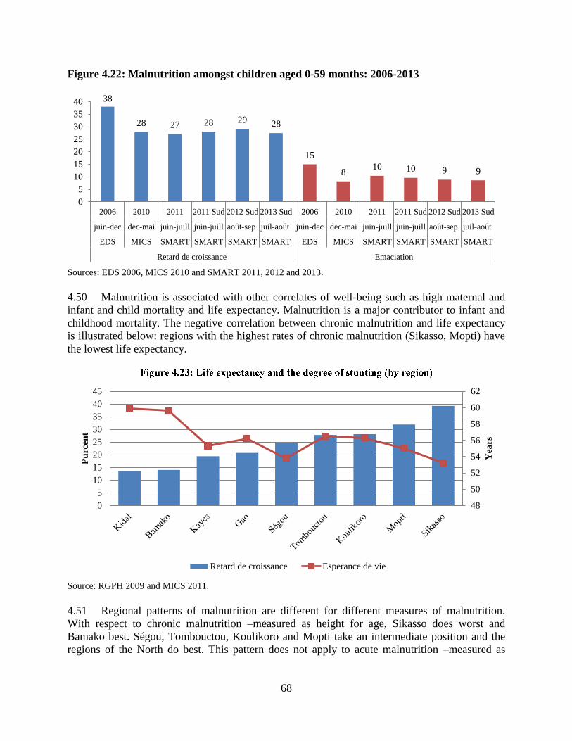
68
Figure 4.22: Malnutrition amongst children aged 0-59 months: 2006-2013
Sources: EDS 2006, MICS 2010 and SMART 2011, 2012 and 2013.
4.50 Malnutrition is associated with other correlates of well-being such as high maternal and
infant and child mortality and life expectancy. Malnutrition is a major contributor to infant and
childhood mortality. The negative correlation between chronic malnutrition and life expectancy
is illustrated below: regions with the highest rates of chronic malnutrition (Sikasso, Mopti) have
the lowest life expectancy.
Source: RGPH 2009 and MICS 2011.
4.51 Regional patterns of malnutrition are different for different measures of malnutrition.
With respect to chronic malnutrition –measured as height for age, Sikasso does worst and
Bamako best. Ségou, Tombouctou, Koulikoro and Mopti take an intermediate position and the
regions of the North do best. This pattern does not apply to acute malnutrition –measured as
38
28 27 28 29 28
15
8 10 10 9 9
0
5
10
15
20
25
30
35
40
2006 2010 2011 2011 Sud 2012 Sud 2013 Sud 2006 2010 2011 2011 Sud 2012 Sud 2013 Sud
juin-dec dec-mai juin-juill juin-juill août-sep juil-août juin-dec dec-mai juin-juill juin-juill août-sep juil-août
EDS MICS SMART SMART SMART SMART EDS MICS SMART SMART SMART SMART
Retard de croissance Emaciation
48
50
52
54
56
58
60
62
0
5
10
15
20
25
30
35
40
45
Yea
rs
Pu
rcen
t
Retard de croissance Esperance de vie

69
weight for height. Now Sikasso is amongst the best performers, while the Northern regions Gao
and Tombouctou (but not Kidal) do worst.
4.52 Poor diets (quantity as well as quality), inadequate caring practices and unhealthy living
environments are generally the major factors contributing to chronic malnutrition, while an
urgent lack of food is the main driver of acute malnutrition. Hence it may be less surprising that
a region like Sikasso (zones 10, 11 and 12) with high agricultural potential faces the highest level
of chronic malnutrition in the country. Demands on labor are high (less time for child care), per
capita of incomes are low and the diet is short on milk and livestock products: even the
wealthiest households consume very little of this (see chapter 3).
4.53 Acute malnutrition is more closely correlated with an urgent inability to access food:
either from one’s own production or through purchases. In a normal agricultural year like 2011,
overall levels of acute malnutrition should be relatively low. The fact that they are still high in
Gao and Tombouctou underscores how during the lean season when food prices are high and
prices for livestock low, when opportunities for gainful employment are limited, poor households
in this zone, are vulnerable and susceptible to acute malnutrition.
4.54 Differing spatial patterns for different types of malnutrition implies different correlations
with income poverty. Hence one finds a high and positive correlation between income poverty
and chronic malnutrition, a correlation that does not exist for acute malnutrition, for which the
most vulnerable populations live in Northern Mali (but not Kidal).
Source: EMOP 2011 and MICS 2011.
4.55 To more formally explore the effect of livelihood zone on consumption per capita we
present a regression in which consumption depends on (1) household demographic
characteristics, which affect household consumption choices, (2) the occupation of household
0
10
20
30
40
50
60
70
80
0
5
10
15
20
25
30
35
40
45
Yea
rs
Po
ver
ty i
nci
den
ce
Retard de croissance Emaciation Taux de pauvrete

70
members, which determines household income, and (3) local characteristics, which influences
choice sets. The model can be written as follows:
𝑙𝑜𝑔𝐶ℎ = 𝐻ℎ′𝜹 +∑ 𝛾𝑗
𝑗𝟙𝑤(ℎ)=𝑗 +∑ 𝜃𝑙
𝑙𝟙𝑧(ℎ)=𝑙 +∑ 𝜌𝑙
𝑙𝟙𝑧(ℎ)=𝑙𝟙𝑤(ℎ)=𝐴𝐺𝑅 + 𝐿𝑐(ℎ)
′ 𝜶 + 𝜖ℎ
where 𝐶ℎ is of per capita consumption expenditure for household h. 𝐻ℎ is a vector of
demographic characteristics of the household, including demographic and educational
characteristics of the household head (with 𝜹 the corresponding vector of coefficients). The
occupation of the household head is given by a set of indicator variables 𝟙𝑤(ℎ)=𝑗 (equal to 1 if
the household head in household h works in occupation 𝑤(ℎ) = 𝑗 and 0 otherwise). The
coefficient 𝛾𝑗 thus measures how consumption per head varies for different professions. 𝟙𝑧(ℎ)=𝑙
is a dummy variable indicating livelihood zone 𝑙 (it is equal to one is 𝑧(ℎ) = 𝑙 and 0 otherwise)
and it is interacted with another dummy variable 𝟙𝑤(ℎ)=𝐴𝐺𝑅 which takes the value 1 if the
household head is working in agriculture and 0 otherwise. Therefore, the estimates of our
coefficients of interest 𝜃𝑙and 𝜌𝑙 shed light on the possible effect of livelihood zones on
consumption for people with non-agricultural occupations and for people working in agriculture
respectively. The vector 𝐿𝑐(ℎ) further introduces local controls at the commune level which may
affect consumption in ways not related to the livelihood zone, such as variations in the presence
of public services. Although the model has as many controls as possible, we cannot completely
rule out endogeneity, in particular that which is related to sorting of household across zones on
unobservables that would impact consumption. The results should thus be interpreted more in
terms of correlation than causation.
4.56 The results are presented in Table 3.2. We first present the model without commune
controls (columns 1 and 2) and then add commune controls (columns 3 and 4). In columns 1 and
3, the interaction terms between livelihood zones and agricultural occupation is dropped. Most
of the estimated coefficients remain stable across model specifications, including the effects of
livelihood zones. Our preferred specification is the complete model which is presented in
column (4).42
4.57 We find that consumption is higher if the household head is male. The estimated
coefficient on gender reflects a 7 percent increase in the per-capita consumption of male headed
households compared to those headed by females. Household consumption decreases with age
of the household head.43
Education of the household head has an important impact on per-capita
consumption. Compared to the benchmark group (those with primary education), per-capita
consumption for households headed by college graduates is about 41 percent higher. We
interacted the education variables with livelihood zone dummies to explore whether returns
differed by zone. The results –not presented here, demonstrate no differences in returns to
education by zone, with the exception of zone 1 where the return to education was higher than
elsewhere.
4.58 Not surprisingly –and in confirmation with the finding by the livelihoods approach that
large households are wealthier, the number of labor-force participants in the household increases
per-capita consumption, whereas having more children or additional old household members in
42
To shorten the table, coefficients on commune level local controls and ethnic groups are omitted from the table. 43
Although the relation is convex, the negative effect dominates for any plausible age.

71
the household decreases consumption. Urban residents consume significantly more compared to
their rural counterparts.
4.59 The estimated coefficients on the occupational controls reflect the ranking of expected
incomes for occupations in Mali. Compared to the benchmark group (people who work in
agriculture), those working in mining, commerce, finance, public administration, health and
extraterritorial organization enjoy noticeably higher per-capita consumption. This reflects better
skilled jobs, opportunities for profit, and shortages in some sectors such as health occupations.44
On the contrary, the advantage from working in education is not as high.
4.60 Addition of commune controls in the regression (columns 3 and 4) reduces the magnitude
and significance of the estimated coefficients on livelihood zones—which are the focus of our
regression. Therefore, in what follows, we only comment on columns 3 and 4. Noticing that
zone 10 (Sorghum, millet, and cotton) had the lowest household per-capita consumption on
average, we selected it to be the comparator. Column 3 reports the results for the model with
commune controls only. We find that there are 10 out of 12 zones with significantly higher
household per-capita consumption levels. Residing in zone 12 (South-west maize, sorghum, and
fruits) provides the smallest significant increase compared to the benchmark zone, with a per-
capita consumption that is higher by 18.2 percent. The largest increases are for zone 8 (North-
west remittances, sorghum, and transhumant livestock rearing) and 13 (Bamako), which has
household per-capita consumptions that are higher by 62 percent and 58 percent respectively.
4.61 Introducing interaction terms between zones and the agricultural occupation dummy for
the household head provides a decomposition of the increase in per-capita consumption by zone
accruing to agricultural and non-agricultural households. We find that many zone coefficients
that were previously significant become insignificant, suggesting that residing in these zones
does not affect non-agricultural households. In zone 8 and zone 13 however, the level effects
(for non-agricultural households) remains significant at the 1 percent although their magnitude is
reduced to 41 percent and 45 percent. Interestingly, interaction terms in 7 and 2 regions out of
13 are significant at the 5 percent and 10 percent level respectively. In zone 5 in particular, per-
capita consumption for households whose household head works in the agricultural sector is 40
percent greater than that of the benchmark zone while the per-capita consumption of non-
agricultural households is no different than that of the benchmark zone. The significance of
these interaction terms combined to the lack of significance in the levels suggests that in many
zones in Mali, differences in consumption levels between zone are driven by different returns to
those working in agriculture.
4.62 In summary, the regression analysis shows important geographic differences in
household consumption, especially across livelihood zones. The capital area, Bamako, and zone
8 (North-west remittances, sorghum, and transhumant livestock rearing) have the highest
household consumption level, an effect which is driven both by agricultural and non-agricultural
activities.
44
There is roughly 1 hospital or clinic available for every 100,000 people in Mali (source: ODHD 2008).

72
(Dependent variable: log per capita consumption in 2001 monetary value)
(1) (2) (3) (4)
Household characteristics:
Gender 0.0799*** 0.0750*** 0.0745*** 0.0721***
Age of household head -0.00978*** -0.00990*** -0.0102*** -0.0103***
Age squared 0.0000761*** 0.0000780*** 0.0000796*** 0.0000815***
Education: Middle school 0.0733** 0.0744** 0.0750*** 0.0756***
Education : High school 0.215*** 0.220*** 0.210*** 0.215***
Education: Advanced 0.415*** 0.420*** 0.405*** 0.413***
Education unreported -0.0785*** -0.0724*** -0.0705*** -0.0648***
# of people under 14 -0.0407*** -0.0402*** -0.0396*** -0.0393***
# of people in labor force 0.00849*** 0.00824*** 0.00725*** 0.00715***
# of elderly -0.0254** -0.0252** -0.0227* -0.0230**
Urban residence 0.216*** 0.203*** 0.0877 0.0709
other than Bamako
Occupational controls:
Fishing 0.0348 0.190** 0.0111 0.204**
Mining 0.373*** 0.515*** 0.341*** 0.527***
Manufacturing 0.151*** 0.300*** 0.131*** 0.316***
Utilities 0.0374 0.180* 0.0113 0.194*
Construction 0.129*** 0.272*** 0.0987*** 0.280***
Commerce 0.246*** 0.389*** 0.209*** 0.391***
Hotel 0.212*** 0.360*** 0.179** 0.365***
Transportation 0.208*** 0.347*** 0.160*** 0.341***
Finance 0.326*** 0.453*** 0.287*** 0.454***
Real estate 0.204*** 0.340*** 0.163** 0.341***
Public administration 0.278*** 0.415*** 0.243*** 0.418***
Education 0.0407 0.180** 0.0224 0.200**
Health 0.265*** 0.408*** 0.242*** 0.421***
Collective self employment 0.166*** 0.314*** 0.129*** 0.315***
Employs domestic workers 0.175*** 0.332*** 0.148*** 0.341***
International organization 0.261* 0.396** 0.249* 0.420***
Employment unreported 0.206*** 0.329*** 0.171** 0.332***
Livelihood zones:
Zone 1 0.0477 -0.0321 0.0955 -0.018
Zone 2 0.272*** 0.164* 0.261*** 0.119
Zone 3 0.193*** -0.00559 0.190** -0.0179
Zone 4 0.0295 -0.147 0.02 -0.180*
Zone 5 0.412*** 0.132 0.397*** 0.108
Zone 6 0.226*** 0.117 0.212*** 0.0895
Zone 7 0.317*** 0.163 0.262*** 0.104
Zone 8 0.625*** 0.451*** 0.617*** 0.416***
Zone 9 0.207*** 0.108 0.194*** 0.0548
Zone 11 0.228*** 0.173** 0.195*** 0.106
Zone 12 0.199*** 0.0832 0.182** 0.0362

73
(1) (2) (3) (4)
Zone 13 0.732*** 0.628*** 0.582*** 0.453***
Livelihood zone interacted with AGR:
Zone 1*AGR
0.0891
0.127
Zone 2*AGR
0.156
0.195*
Zone 3*AGR
0.281***
0.288***
Zone 4*AGR
0.241**
0.267***
Zone 5*AGR
0.387***
0.396***
Zone 6*AGR
0.156**
0.162*
Zone 7*AGR
0.223**
0.237**
Zone 8*AGR
0.240***
0.270***
Zone 9*AGR
0.142*
0.195**
Zone 11*AGR
0.0609
0.113
Zone 12*AGR
0.163
0.202*
Zone 13*AGR
0.261***
0.268***
Constant 11.82*** 11.79*** 11.74*** 11.70***
Ethnic group controls Y Y Y Y
Local characteristics
controls N N Y Y
Observation 9036 9036 9036 9036
R-squared 0.53 0.533 0.538 0.541
*** significant at 1% level, ** significant at 5% level, * significant at 10% level
Source: ELIM 2010. Authors’ calculations
4.63 This chapter discussed the importance of spatial characteristics, and particular livelihood
zones, for welfare. Urban households do much better than rural households, explaining in part
the attractiveness of urban areas for migrants. Amongst rural households the pattern that emerges
is that households in livelihood zone 10 –those growing sorghum, millet and cotton in the
Sikasso region are amongst the most destitute in the country. Relative to the rest of the nation,
their consumption is amongst the lowest, as is life-expectancy while levels of chronic
malnutrition and poverty are amongst the highest. In terms of other indicators Sikasso appears to
be doing better: acute malnutrition is relatively low in Sikasso, and the ownership of assets and
consumer durables is relatively elevated.
4.64 Increasing remittances and increases in the production of cereals, of maize and rice in
particular, have driven the rapid poverty reduction that occurred between 2001 and 2010. The
poorest households have benefited most from this. Improvements in welfare are strongly
associated with livelihood zones relying on remittances (zone 8 in north-west Kayes), zones 11
and 12 in South Sikasso, zones 3 and 6 (producing rice on the borders of the Niger or as part of
the office du Niger) and to a lesser degree zone 9 (west and central), producing millet and
sorghum under rain-fed conditions. Households depending on livestock rearing in zone 2 in the
regions of Gao and Tombouctou and those in the Niger delta (zone 6) have not been doing well.
4.65 Bamako and Kidal are the regions where households are best off in terms of
consumption, though the situation in Kidal can be expected to have changed dramatically as a
result of the security crisis.

74
4.66 There are a number of implications to be derived from the chapter. Mali has a
comparative advantage to serve the region with food (see also chapter 6 on growth) and there
seems to be potential for maize and rice to production to increase. To make this happen it is
important to ensure that these products can effectively be exported otherwise increases in
production might lead to declines in prices and incomes. With the continuing crisis in the North,
this may not be self-evident as it is unclear whether the highway to Gao is secure.
4.67 The elevated levels of poverty in livelihood zone 10 remain somewhat of a puzzle. The
agricultural potential of this zone is high. In part because of its association with cotton, market
accessibility and the availability of inputs are also relatively good in this zone. It may be that the
high levels of poverty are an artefact of the data because data collection for ELIM 2010
coincided with a period of adverse weather in this zone. Never the less, given the success of
maize production elsewhere and the high fluctuations in the value of cotton production, one
wonders–but additional research would have to clarify this, whether it is possible to expand
maize production in this zone, or alternatively what is the potential to increase sorghum and
millet production.
4.68 Zones 3 (on the borders of the Niger between Gao and Tombouctou and 7 -Office du
Niger) already benefited from increases in rice production and, the security situation allowing,
there seems to be potential to increase the production of rice in the Niger delta (zone 3). Doing
so requires improving market accessibility as this zone is affected by poor market access.
4.69 The long run policy implication that follows from this chapter is a huge need to invest in
education. Returns to education are high. Even though this is partly reflects the scarcity of
educated people, it is unimaginable for sustainable growth to occur without addressing the huge
education deficit. Doing so will require actions now that can only be expected to yield a return in
10 to 15 years’ time.
4.70 Important lessons can be learned from the success of households in zone 8 in north-west
Kayes who through migration and reliance on remittances have managed to build secure and
improving livelihoods. There is a clear link with education, as better educated migrants are more
likely to succeed–as discussed in chapter 2.
4.71 According to the ‘traditional’ poverty measure 70 percent of all poor are located in three
livelihood zones: 9 (west and central rain-fed millet/sorghum), 10 (sorghum, millet and cotton)
and 11 (south, maize, cotton and fruits). The case to focus policy interventions on households in
zone 10 is particularly strong because many households live in this zone, because the incidence
of poverty is high and because, unlike zones 9 and 11 poverty levels have been increasing. Zone
4, where 10 percent of poor households live, also deserves additional attention even though the
much lower population density of this zone might hinder the design of cost-effective
interventions. These results need to be interpreted with caution, however, as the asset based
poverty measure (presented in Figure 4.16) suggests that poverty is much more equally spread
across southern Mali.
4.72 Finally the north has been badly affected by the security crisis. A trade-off seems to have
to be made between efficiency (the north has low population density) and need. However, there
are many more aspects to interventions in the north than this simple trade-off. It is clear that
important spillover effects have occurred from the crisis in the north as consumption levels have

75
fallen throughout the country since 2011 (with the exception of Bamako) and not just in the
north: finding a solution to the crisis in the north is in the interest of all.
76
Spatial Challenges to Service Delivery: Trading
off Equity, Efficiency and Quality
5.1 In this chapter we focus on service delivery. Services come in many forms and include
social services such as health, water and education, economic services such as roads, markets,
banks and electricity, information services (radio, television, telephone) as well as security
services (police, military) or cultural services (sports facilities, theater). Not all services are
provided by the public sector but many are. For services that are provided by the private sector –
as is for instance the case with mobile telephony, or rural electricity, the public sector often plays
an important regulatory role.
5.2 In previous chapters we noted how geographic differences have important consequences
for livelihood choices, which in turn are closely associated to different levels of welfare. In this
chapter we focus on the consequences of spatial aspects for the provision of services. In this
instance we focus less on the livelihood zone, but more on the differences in population density
and how it forces decision makers to choose between access for all (equity) and efficiency
(providing access to as many people as possible for a given budget).
5.3 We illustrate this point with three examples: primary education, electricity and access to
markets. Each of these services faces its own trade-offs. For primary education in 2009 there
were almost 11,000 villages (Table Annex 2.3) and approximately 4,500 schools so in addition
to the challenge that every village cannot be served by a school, a trade-off exists between
improving access and improving quality. In electricity the trade-off is about whom to give
access: the urban rich or the rural poor. With respect to access to markets, finally, in addition to
access and efficiency issues, we again note that quality issues (road blocks, maintenance
planning) are critical. For all three services we show how innovations –from the introduction to
double shifting in schools, to solar lights and cheap motor bikes, help make certain trade-offs
more palatable.
5.4 Unit costs, which are the costs that need to be made before a service can be offered,
matter a great deal for whether a service can be offered, or in how many places a service can be
offered efficiently. Unit costs, in turn, are largely determined by the size of fixed costs: services
requiring large upfront investments such as piped water or electricity can only be offered in a
cost-effective manner in areas where population density is high: cities. How pressing this
problem is can be illustrated with an example for secondary schools. Imagine that the maximum
distance a secondary student can be expected to travel is 7 km (one way), and that a secondary
school requires at least 250 students to be cost-efficient. Moreover, assume that 30 out of every
100 children complete primary school (see section 5.2). Children of secondary school age (those
aged 13-18) make up 14 percent of the population.45
The catchment area of a school is 154 km2
45
Estimated using 2009 census data.
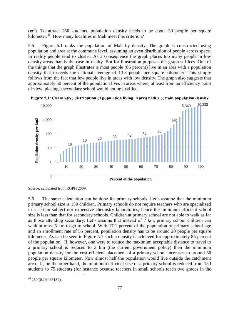
77
(πr2). To attract 250 students, population density needs to be about 39 people per square
kilometer.46
How many localities in Mali meet this criterion?
5.5 Figure 5.1 ranks the population of Mali by density. The graph is constructed using
population and area at the commune level, assuming an even distribution of people across space.
In reality people tend to cluster. As a consequence the graph places too many people in low
density areas than is the case in reality. But for illustration purposes the graph suffices. One of
the things that the graph illustrates is most people (85 percent) live in an area with a population
density that exceeds the national average of 13.3 people per square kilometer. This simply
follows from the fact that few people live in areas with low density. The graph also suggests that
approximately 50 percent of the population lives in areas where, at least from an efficiency point
of view, placing a secondary school would not be justified.
Source: calculated from RGPH 2009.
5.6 The same calculation can be done for primary schools. Let’s assume that the minimum
primary school size is 150 children. Primary schools do not require teachers who are specialized
in a certain subject nor expensive chemistry laboratories; hence the minimum efficient school
size is less than that for secondary schools. Children at primary school are not able to walk as far
as those attending secondary. Let’s assume that instead of 7 km, primary school children can
walk at most 5 km to go to school. With 17.1 percent of the population of primary school age
and an enrollment rate of 55 percent, population density has to be around 20 people per square
kilometer. As can be seen in Figure 5.1 such a density is achieved for approximately 85 percent
of the population. If, however, one were to reduce the maximum acceptable distance to travel to
a primary school is reduced to 3 km (the current government policy) then the minimum
population density for the cost-efficient placement of a primary school increases to around 50
people per square kilometer. Now almost half the population would live outside the catchment
area. If, on the other hand, the minimum efficient size of a primary school is reduced from 150
students to 75 students (for instance because teachers in small schools teach two grades in the
46
250/(0.14*.3*154).
10 19
26 33 42 54 80
469
5,340 10,332
0
1
10
100
1,000
10,000
10 20 30 40 50 60 70 80 90 100
Po
pil
ati
on
den
sity
per
km
2
Percent of the population
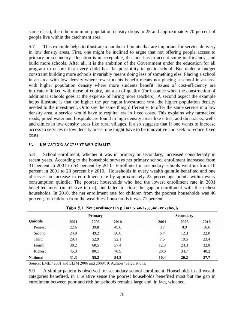
78
same class), then the minimum population density drops to 25 and approximately 70 percent of
people live within the catchment area.
5.7 This example helps to illustrate a number of points that are important for service delivery
in low density areas. First, one might be inclined to argue that not offering people access to
primary or secondary education is unacceptable, that one has to accept some inefficiency, and
build more schools. After all, it is the ambition of the Government under the education for all
program to ensure that every child has the possibility to go to school. But under a budget
constraint building more schools invariably means doing less of something else. Placing a school
in an area with low density where few students benefit means not placing a school in an area
with higher population density where more students benefit. Issues of cost-efficiency are
intricately linked with those of equity, but also of quality (for instance when the construction of
additional schools goes at the expense of hiring more teachers). A second aspect the example
helps illustrate is that the higher the per capita investment cost, the higher population density
needed to the investment. Or to say the same thing differently: to offer the same service in a low
density area, a service would have to require less in fixed costs. This explains why tarmacked
roads, piped water and hospitals are found in high density areas like cities, and dirt tracks, wells
and clinics in low density areas like rural villages. It also suggests that if one wants to increase
access to services in low density areas, one might have to be innovative and seek to reduce fixed
costs.
5.8 School enrollment, whether it was in primary or secondary, increased considerably in
recent years. According to the household surveys net primary school enrollment increased from
31 percent in 2001 to 54 percent by 2010. Enrollment in secondary schools went up from 10
percent in 2001 to 28 percent by 2010. Households in every wealth quintile benefited and one
observes an increase in enrollment rate by approximately 23 percentage points within every
consumption quintile. The poorest households who had the lowest enrollment rate in 2001
benefited most (in relative terms), but failed to close the gap in enrollment with the richest
households. In 2010, the net enrollment rate for children from the poorest households was 46
percent; for children from the wealthiest households it was 71 percent.
Primary Secondary
Quintile 2001 2006 2010
2001 2006 2010
Poorest 22.6 39.8 45.8
3.7 8.9 16.6
Second 24.9 49.2 50.8
6.4 12.3 22.0
Third 29.4 52.9 52.1
7.5 19.5 23.4
Fourth 38.2 60.5 57.4
12.3 24.4 32.8
Richest 45.3 80.1 70.9
20.9 34.7 40.2
National 31.3 55.2 54.3
10.4 20.2 27.7
Source: EMEP 2001 and ELIM 2006 and 2009/10. Authors’ calculations.
5.9 A similar pattern is observed for secondary school enrollment. Households in all wealth
categories benefited, in a relative sense the poorest households benefited most but the gap in
enrollment between poor and rich households remains large and, in fact, widened.

79
5.10 The regional pattern of enrollment is informative of between region differences; we do
consider it in Figure 5.2. The data show the presence of large variations. Using the 2011 EMOP,
which is the last household survey that was fielded in all regions, one observes how enrollment
varies from as low as 35 percent in Tombouctou and Mopti to as high as 83 percent in Bamako.
The Figure also shows the diversity of the North of the country: enrollment is extremely low in
Tombouctou and Mopti while in Gao and Kidal enrollment rates are comparable to elsewhere in
the country.
Source: EMOP 2011 & 2013.
5.11 Noteworthy is that the increase in enrollment has come to a halt. The 2013 EMOP did not
collect information in the north–where as a result of the crisis school enrollment has fallen
dramatically, however it did in south Mali. Its results show how with the exception of Bamako
and relative to 2011 net enrollment rates went down in all regions.
5.12 Figure 5.3 presents the fraction of people living within a certain distance of a school.
Distance is important for school attendance and children who live further from school have a
smaller chance of attending it. A study carried out by DNSI (2007)47
shows how children living
more than 45 minutes from the nearest school are more than twice as likely not to attend school,
than those who live less than 30 minutes away from school. The Figure shows that depending on
where one lives between 92 and 100 percent of people live within 5km of a primary school, with
the exception of households in Mopti and Tombouctou where between 82 and 86 percent live
within 5 km of a school. 5 km is quite a distance to cover –particularly for young children, which
is why we also present the fraction of the population living within 2 km. Again, the vast majority
of the population (more than 80 percent) lives within 2km of a school, but in Kidal, Tombouctou
and Mopti the percentage is significantly lower: around two-third live within 2 km of a school.
47
DNSI 2007. Pauvreté et Education au Mali: les determinants de la frequentation scolaire.
63 64 66 59
36 35
68 66
83
60 60 54
59 50
35
92
0102030405060708090
100
Per
cen
t
2011 2013

80
Source: EMOP 2011 (enrollment) and RGPH 2009 (distance). Authors’ calculations.
5.13 Distance is obviously not the only factor explaining low attendance in Mopti and
Tombouctou. In fact, with more than 60 percent of the population living within two kilometers of
a school, attendance rates could be substantially higher than the 35 percent reported in Figure
5.2. Also in other regions, Kayes, Koulikoro, Sikasso and Ségou shows the difference between
the fraction of the population that lives close to a school and the net enrollment rate significant.
In other words, even without constructing any new schools attendance rates could be much
higher. This is not to state that no new school construction should take place. Mapping the
information available and creating a 5km radius around every school (Figure 5.4) demonstrates
that certain localities do not benefit from a primary school, even though population density in the
area is relatively high. Such areas deserve to be targeted for new school construction.
5.14 To further explore the overall spatial allocation of schools, classroom and teachers we use
the data presented in Table 5.2, to calculate how many additional (fewer) schools a region should
have if every region was at the national average. Doing this suggests that Bamako, Ségou and
Mopti should receive additional schools, classrooms and teachers while Kidal, Koulikoro, and
particularly Sikasso, Kidal and Gao should receive less. This, however, just presents a first
approximation as many other variables determine whether a region should get additional or less
resources. Population density in Bamako is so high (and the cost of land so elevated) that it
makes sense to have fewer but larger schools. Enrollment rates in Mopti are so low, that it may
make sense to expect teachers to teach multiple grades at the same time. So few people live
within 2km of a school in Gao, Tombouctou and Kidal that it makes sense to put relatively more
schools in these regions. It also makes sense for these schools to be relatively small. Indeed the
63 64 66 59
36 35
68 66
83
86 90 90
82
70 64
87
67
93 97 97 97
86 82
97 92
100
0
10
20
30
40
50
60
70
80
90
100
0
10
20
30
40
50
60
70
80
90
Per
cen
t li
vin
g w
ith
in 5
km
of
sch
oo
l
Net
en
roll
men
t ra
te
Taux net de scolarisation Living less than 2 km from school
Living less 5km from school (RGPH 2009)
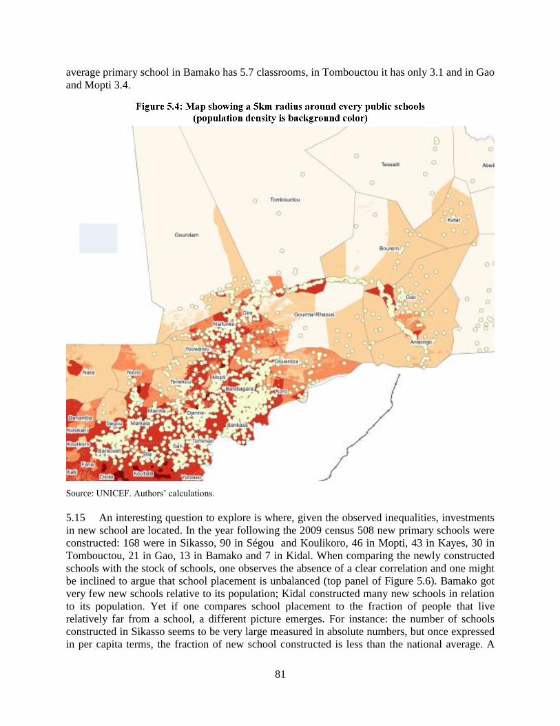
81
average primary school in Bamako has 5.7 classrooms, in Tombouctou it has only 3.1 and in Gao
and Mopti 3.4.
Source: UNICEF. Authors’ calculations.
5.15 An interesting question to explore is where, given the observed inequalities, investments
in new school are located. In the year following the 2009 census 508 new primary schools were
constructed: 168 were in Sikasso, 90 in Ségou and Koulikoro, 46 in Mopti, 43 in Kayes, 30 in
Tombouctou, 21 in Gao, 13 in Bamako and 7 in Kidal. When comparing the newly constructed
schools with the stock of schools, one observes the absence of a clear correlation and one might
be inclined to argue that school placement is unbalanced (top panel of Figure 5.6). Bamako got
very few new schools relative to its population; Kidal constructed many new schools in relation
to its population. Yet if one compares school placement to the fraction of people that live
relatively far from a school, a different picture emerges. For instance: the number of schools
constructed in Sikasso seems to be very large measured in absolute numbers, but once expressed
in per capita terms, the fraction of new school constructed is less than the national average. A

82
lower construction rate than the national average seems appropriate given the fact that Sikasso
already has more schools per citizen than the average for the country. Also the fraction of people
living within 2km of a school is higher in Sikasso than the average for the nation. Based on these
latter grounds, one could have argued for even less schools per capita to be constructed in
Sikasso. Kidal, on the other hand, got the same number of additional schools as the national
average, but based on the fraction of the population living close to a school, it could have
received some more. This contrary to Ségou, which received –in per capita terms, many schools
in an environment where the number of schools per capita was already much higher than the
national average and where the fraction of people living close to a school also exceeds the
national average.
Source: Ministry of Education Statistical Abstract. Authors’ calculations.
5.16 We also related new school construction to the number of additional students; we
considered classroom construction and the placement of teachers and repeated the exercise for
secondary schools. In all instances we do find sizeable regional differences, but no evidence of
gross misallocations or of one region being favored over another.
(1,500)
(1,000)
(500)
-
500
1,000
1,500
2,000
Ecoles Salles Groupes
Pédagogiques
Maîtres
chargés de
cours

83
Source: Ministry of education, statistical yearbooks. Authors’ calculations.
5.17 Education is not about facilities but about learning; teachers are indispensable for this
outcome. Unlike the number and allocation of schools across the country, the school system
faces serious challenges with the total number of teachers and their distribution across the
country. The total number of teachers is low as evidenced by the student – teacher ratio for the
country in 2010/11 (Table 5.2): 60 to 1 (45 to 1 is generally considered an upper bound of what
is acceptable). The average hides significant variation, which becomes already clear when
0
0.02
0.04
0.06
0.08
0.1
0.12
0
0.1
0.2
0.3
0.4
0.5
0.6
0.7
New
sch
oo
ls
Sch
oo
ls
Ecoles par '000 habitants Nouvelles ecoles par '000 habitants
0
10
20
30
40
50
60
70
80
90
100
0
0.02
0.04
0.06
0.08
0.1
0.12
Po
urc
en
t
New
sch
oo
ls
Moins de 2km d'une ecole Nouvelles ecoles par '000 habitants

84
considering the regional level. The student – teacher ratio varies from as low as 35 to 1 in Kidal
to as much as 73 to 1 in Bamako. These extremes are partly explained by population density as
in Kidal there are relatively few students per grade - consequently student teacher ratios are low.
In Bamako the reverse is the case.
5.18 Increasing the number of teachers –or for that matter increasing the number of
classrooms as also the number of students per classroom is very high, seems to be a matter of
policy priority even though it may be difficult to achieve in the short run, for both budgetary
reasons and because sufficient trained teachers are simply not available. This raises an issue
whether there might be other solutions –innovations if one likes, to this problem. Such
innovations do exist: for instance, constrained by the number of classrooms and the number of
available teachers, the authorities could consider the introduction of double shift system in which
teachers teach two classes on the same day: one in the mornings and one in the afternoon.
Needless to say, teachers would probably need to be paid extra in order to motivate them.
Alternatively, if a double shift system is too demanding for the current teachers, the system could
be introduced while hiring additional teachers (from neighboring countries?). Other innovations
need to be considered as well. In a context of hard budgetary constraints and major challenges,
the choice is between innovation and the non-delivery of the service.
5.19 Associated to the presence of sufficient teachers is the need to ensure quality. A huge
challenge lies here. Education experts consider any child who does not complete at least grade 5
a loss, which means that the child is considered not to have learned enough to contribute
significant economic value to society during the rest of the child’s life. Hence, it is important that
those children that enter the education system complete at least five years of education. This is
often not the case. Figure 3.6 shows that 63 percent of all children complete at least grade 1
(suggesting that 37 percent do not go to school at all) and that of these only 59 percent complete
grade 2. By the time one arrives at grade 5 only 41 out of every 100 children have managed to
complete this level. In other words, compared to a situation in which the 63 percent who attend
the first year of primary school were retained, 44 percent48
of all spending on children in grades
one to five can be considered a use of resources with little (economic) return on investment.
5.20 We conclude that progress has been made in enhancing access in the education sector.
With over 10,000 villages and approximately 5,000 schools, it is clear that choices have to be
made and that not every village can be served by a primary school and when they do get a
primary school it may be a one classroom school, or a school with multigrade teaching.
5.21 We also find that the education system is relatively balanced with respect to the
distribution of schools across regions. There are areas in which new schools need to be placed to
ensure access, but overall the evidence does not give reason to believe that one region is
structurally favored over another or that the placement of schools is seriously skewed.
48
Calculated as (34.9/62.7)-1.
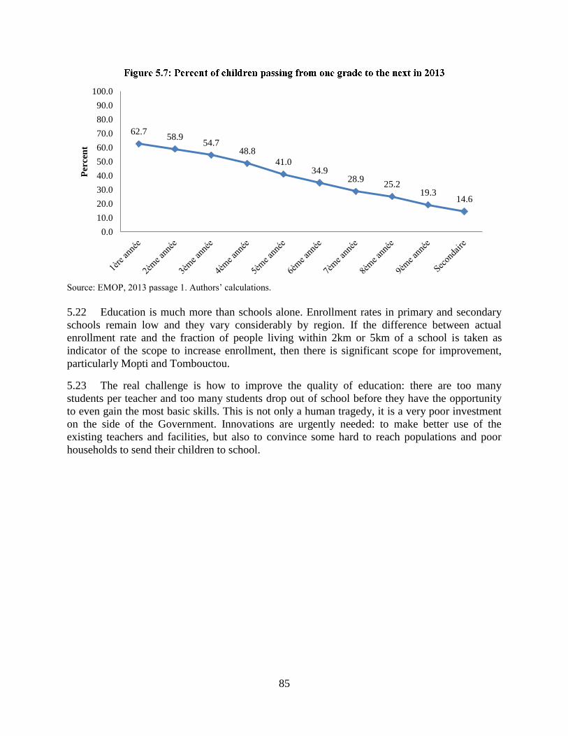
85
Source: EMOP, 2013 passage 1. Authors’ calculations.
5.22 Education is much more than schools alone. Enrollment rates in primary and secondary
schools remain low and they vary considerably by region. If the difference between actual
enrollment rate and the fraction of people living within 2km or 5km of a school is taken as
indicator of the scope to increase enrollment, then there is significant scope for improvement,
particularly Mopti and Tombouctou.
5.23 The real challenge is how to improve the quality of education: there are too many
students per teacher and too many students drop out of school before they have the opportunity
to even gain the most basic skills. This is not only a human tragedy, it is a very poor investment
on the side of the Government. Innovations are urgently needed: to make better use of the
existing teachers and facilities, but also to convince some hard to reach populations and poor
households to send their children to school.
62.7 58.9
54.7 48.8
41.0 34.9
28.9 25.2
19.3 14.6
0.0
10.0
20.0
30.0
40.0
50.0
60.0
70.0
80.0
90.0
100.0P
erce
nt
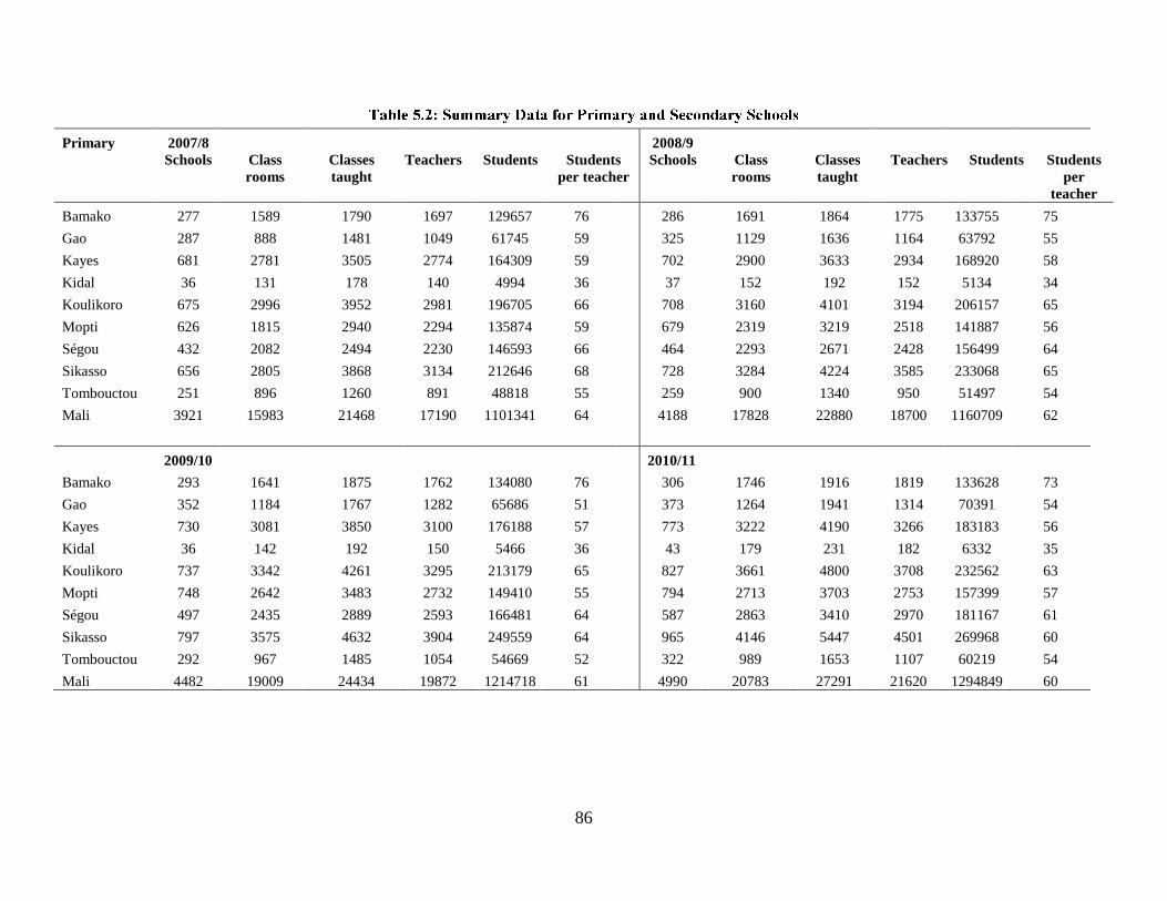
86
Primary 2007/8
2008/9
Schools Class
rooms
Classes
taught
Teachers Students Students
per teacher
Schools Class
rooms
Classes
taught
Teachers Students Students
per
teacher
Bamako 277 1589 1790 1697 129657 76
286 1691 1864 1775 133755 75
Gao 287 888 1481 1049 61745 59
325 1129 1636 1164 63792 55
Kayes 681 2781 3505 2774 164309 59
702 2900 3633 2934 168920 58
Kidal 36 131 178 140 4994 36
37 152 192 152 5134 34
Koulikoro 675 2996 3952 2981 196705 66
708 3160 4101 3194 206157 65
Mopti 626 1815 2940 2294 135874 59
679 2319 3219 2518 141887 56
Ségou 432 2082 2494 2230 146593 66
464 2293 2671 2428 156499 64
Sikasso 656 2805 3868 3134 212646 68
728 3284 4224 3585 233068 65
Tombouctou 251 896 1260 891 48818 55
259 900 1340 950 51497 54
Mali 3921 15983 21468 17190 1101341 64
4188 17828 22880 18700 1160709 62
2009/10
2010/11
Bamako 293 1641 1875 1762 134080 76
306 1746 1916 1819 133628 73
Gao 352 1184 1767 1282 65686 51
373 1264 1941 1314 70391 54
Kayes 730 3081 3850 3100 176188 57
773 3222 4190 3266 183183 56
Kidal 36 142 192 150 5466 36
43 179 231 182 6332 35
Koulikoro 737 3342 4261 3295 213179 65
827 3661 4800 3708 232562 63
Mopti 748 2642 3483 2732 149410 55
794 2713 3703 2753 157399 57
Ségou 497 2435 2889 2593 166481 64
587 2863 3410 2970 181167 61
Sikasso 797 3575 4632 3904 249559 64
965 4146 5447 4501 269968 60
Tombouctou 292 967 1485 1054 54669 52
322 989 1653 1107 60219 54
Mali 4482 19009 24434 19872 1214718 61
4990 20783 27291 21620 1294849 60
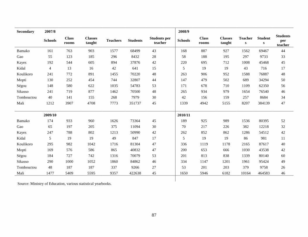
87
Secondary 2007/8
2008/9
Schools Class
rooms
Classes
taught Teachers Students
Students per
teacher Schools
Class
rooms
Classes
taught
Teacher
s
Student
s
Students
per
teacher
Bamako 161 763 903 1577 68499 43
168 887 927 1562 69467 44
Gao 55 123 185 296 8432 28
58 188 195 297 9733 33
Kayes 192 544 605 894 37876 42
220 695 712 1008 45468 45
Kidal 4 13 16 42 641 15
5 19 19 43 716 17
Koulikoro 241 772 891 1455 70220 48
263 906 952 1588 76887 48
Mopti 130 252 454 744 32807 44
147 479 502 689 34294 50
Ségou 148 580 622 1035 54783 53
171 678 710 1109 62350 56
Sikasso 241 719 877 1462 70500 48
265 934 979 1654 76540 46
Tombouctou 40 141 155 268 7979 30
42 156 159 257 8684 34
Mali 1212 3907 4708 7773 351737 45
1339 4942 5155 8207 384139 47
2009/10
2010/11
Bamako 174 933 960 1626 73364 45
189 925 989 1536 80395 52
Gao 65 197 205 375 11094 30
70 217 226 382 12218 32
Kayes 247 788 802 1213 50990 42
262 852 862 1286 54512 42
Kidal 5 19 19 49 847 17
5 19 19 86 981 11
Koulikoro 295 982 1042 1716 81304 47
336 1119 1178 2165 87617 40
Mopti 169 576 586 865 40832 47
200 653 666 1030 43538 42
Ségou 184 727 742 1316 70079 53
201 813 838 1339 80140 60
Sikasso 290 1000 1052 1860 84862 46
334 1147 1201 1961 95424 49
Tombouctou 48 187 187 337 9266 27
53 201 203 379 9758 26
Mali 1477 5409 5595 9357 422638 45
1650 5946 6182 10164 464583 46
Source: Ministry of Education, various statistical yearbooks.
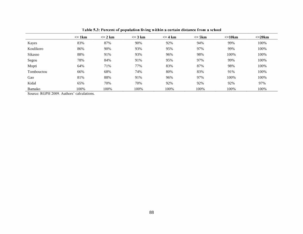
88
<= 1km <= 2 km <= 3 km <= 4 km <= 5km <=10km <=20km
Kayes 83% 87% 90% 92% 94% 99% 100%
Koulikoro 86% 90% 93% 95% 97% 99% 100%
Sikasso 88% 91% 93% 96% 98% 100% 100%
Segou 78% 84% 91% 95% 97% 99% 100%
Mopti 64% 71% 77% 83% 87% 98% 100%
Tombouctou 66% 68% 74% 80% 83% 91% 100%
Gao 81% 88% 91% 96% 97% 100% 100%
Kidal 65% 70% 70% 92% 92% 92% 97%
Bamako 100% 100% 100% 100% 100% 100% 100%
Source: RGPH 2009. Authors’ calculations.

89
5.24 More than education, access to electricity is complicated by the large investments in
generating capacity and a distribution network that it requires. It is unsurprising that access to
electricity is unequal and that access is closely associated to areas with high population density.
As Table 2.4 already demonstrated, only 1 percent of households in villages have access to
electricity, 8 percent in rural towns, 17 percent in towns and about 45 percent of the population
in cities. Access to electricity is highest in Bamako where 68 percent of households have access.
5.25 The ability to use electricity remains a crucial dimension of growth and poverty
reduction. It is encouraging that between 2001 and 2010 access to electricity increased from
about 9 percent nationwide to around 24 percent.49
Urban and rural areas have both seen their
access increase. In urban areas, access has more than doubled from 28 percent in 2001 to 60
percent in 2010. In rural areas it started from a much lower base and access quadrupled (from 2.4
to 11.0 percent). The increase in rural areas remains strongly associated to rural towns; access in
Mali’s 10,000 villages remains negligible.
Source: ELIM 2010. Authors’ calculations.
5.26 The upward trend in access to electricity benefited households in the lower wealth
quintiles more than the richer ones but at 3 percent the poorest households still have much less
access to electricity than better off households: 62 percent of households in the top wealth
quintile have electricity (see Figure 5.8).
5.27 Given the limited access to electricity it is no surprise that the vast majority of formal
enterprises is located in Bamako, and if not in Bamako, then in one of the regional capitals.
49
According to the EMOP 2011 access has increased to 34 percent. Relative to the access reported for 2009/10
based on the ELIM this increase seems very large. In this section we further use the ELIM.
0
50,000
100,000
150,000
200,000
250,000
300,000
Le plus pauvre 2 3 4 Le plus aise
Nu
mb
er o
f h
ou
sheo
lds
Quintile
access Sans access

90
Outside these localities electricity is not available. Even where electricity is available for
productive purposes, it is unreliable. Power surges harm equipment and in certain months
demand exceeds supply (by as much as 13 percent, February being the worst month) and
electricity is rationed through load shedding.
5.28 The challenges facing the electricity sector are threefold. First demand exceeds supply,
necessitating load shedding, which in turn has a negative impact on productivity. For future
growth it is critical that electricity is not a constraint, hence additional investments in generating
capacity are needed. A second problem is that the electricity sector is heavily subsidized. In 2014
alone, a subsidy of FCFA 30 billion has been budgeted to go to EDM. Even with this subsidy,
EDM is expected to make a loss of more than FCFA 5 billion (Government of Mali, 2014). The
third problem is that electricity is not available in rural areas, delaying growth and the reduction
of poverty precisely in areas where most progress is needed.
5.29 The electricity sector focuses most of its attention to solving the first problem and largely
ignores the second and third. But could the (urban) electricity sector not be made financially
sustainable without the need for subsidization, and is equitable access to electricity indeed
impossible?
5.30 To start with the last question: it depends. If the objective is for all households to access
electricity that can be used for productive purposes, and to run heavy equipment like air
conditioners, then inequitable access is likely to persist for a long time as the entire nation would
have to be hooked up to a network. But if the ambition is formulated in a more realistic way and
the objective is for all households to have access to electricity for basic appliances such as
lighting, running a radio or charging a mobile phone, then it may be feasible. The reason being
that to fulfill this ambition limited investments in generating power and a network have to be
made to connect small town while solar powered devices could be offered as an alternative to the
majority of the population who resides in rural areas.
5.31 What about subsidies. Could they be abolished? Doing so requires raising the electricity
tariff (and reducing the efficiency losses) to a level where financial losses are no longer incurred.
Doing so would help reduce the existing capacity problem as private electricity providers may
now want to consider producing and selling electricity to the network (as is the case already in
rural areas).
5.32 Abolishing the subsidy and increasing the electricity tariff could have negative
consequences for enterprises (who face higher costs) and could lead to increases in (urban)
poverty. The impact on enterprises can be expected to be limited as for most spending on
electricity does not make up a large share of their cost: load shedding and power surges are
typically much more costly. The impact on urban poverty has been shown to be limited, because
the share of spending on electricity is limited, because incomes in urban areas are amongst the
highest in the country and because the poorest households have limited access to electricity in
any case. A paper prepared by the World Bank (2013) demonstrates how the effect of a 6.5
percent tariff increase on poverty would be extremely marginal: an increase in poverty incidence
by less than 0.1 percent.50
50
World Bank 2013. The Effect of Electricity Tariff Increases on Poverty and Welfare Distribution in Mali.
91
5.33 Raising electricity tariffs might be politically unpalatable, unless a trade-off is
proposed that is acceptable: like giving access to electricity to the majority of the
population. The subsidy of FCFA 30 – 35 billion envisaged for 2014 is sufficient to provide up
to 1 million solar units, which could be used for lighting, listening to the radio or charging a
mobile phone. One million units would be sufficient to light up rural Mali. Access to a unit could
be made conditional on school enrollment, or on visiting a clinic during pregnancy, thus
achieving multiple objectives at the same time while solving the problem of what to use as
distribution channel. Access to the units would reduce the dependency on kerosene for lighting,
would create new economic opportunities as people can work in the evening, would allow
children to study at night (and do chores after school?), and could even help establish a new
sector of enterprises serving the solar market.
5.34 In conclusion, there are huge challenges associated to providing access to electricity,
which are associated to the high fixed cost of generating and distribution capacity. This section
acknowledges these challenges and accepts that the provision of networked electricity will
largely be limited to high density, urban areas. At the same time, it is argued that if the objective
is to reduce poverty, existing ways of doing business may have to be reviewed and innovative
and affordable approaches embraced.
5.35 Limited market access affects households in multiple ways. In chapter two we argued that
that the high cost of inter-city transport and communication contributes to a lack of specialization
between cities. Poor and non-poor households benefit from roads through the access they provide
to services in areas such as health, education, agricultural extension, and provision of
information. Improved access to markets also means improved economic opportunities. In rural
areas it means opportunities to sell produce from the harvest or livestock and to purchase food
and other consumer goods.
5.36 For people living in rural areas poor market access implies that prices obtained for
agricultural produce are relatively low, while prices for products that are purchased are relatively
high, which not only makes the cost of inputs higher, but also raises the prices of consumer
goods bought with the money earned. High transport cost thus leads to poor ‘terms of trade’ for
rural households and contributes to a decrease in the return to labor, which discourages the use of
modern inputs and the production of a surplus and makes it rational for households to opt for
subsistence agriculture. A recent study on Sub-Saharan Africa has shown that production areas
that are nine hours away from the market realize only 8 percent of their agricultural potential,
while those located four hours away from the market realize 46 percent of their potential.51
Hence, to enhance the agricultural production and rapidly reduce poverty, it is imperative that the
distance between markets and households is reduced.
51
Clesensio Tizikara and Loro George Leju Lugor, MAFCRD Post Conflict Development of Agriculture in South
Sudan, perspective on approaches to capacity strengthening. Juba 2012.

92
Source: RGPH 2009. Authors’ calculations.
5.37 In order to explore which localities in the country have good market access, a market
accessibility indicator was estimated following a methodology described by Deichmann (1997)52
and Nelson (2008).53
The approach estimates travel time from assumptions of speed on the road
network based on road category (primary, secondary and tertiary) and then identifies the
accessibility index as the sum of the population of urban/village centers in the vicinity of each
point in the country, weighted inversely by the time of travel on the transportation network to
each urban center along the road network. The index presented on a map in Figure 5.9, was
calculated with the negative exponential potential model54
with village level population from the
52
Deichmann, U. (1997). Accessibility indicators in GIS. United Nations Statistics Division. 53
Nelson, A. (2008). Travel time to major cities: A global map of Accessibility. Global Environment Monitoring
Unit - Joint Research Centre of the European Commission, Ispra Italy. Available at http://gem.jrc.ec.europa.eu/ 54
The market accessibility index is calculated with the negative exponential potential model. The following
parameters are in the accessibility model: cost-distance threshold = 3 hours, cost/distance decay exponent for the
negative exponential model of 1.5; and cost/distance to the point of inflection of the distance decay function at 90;
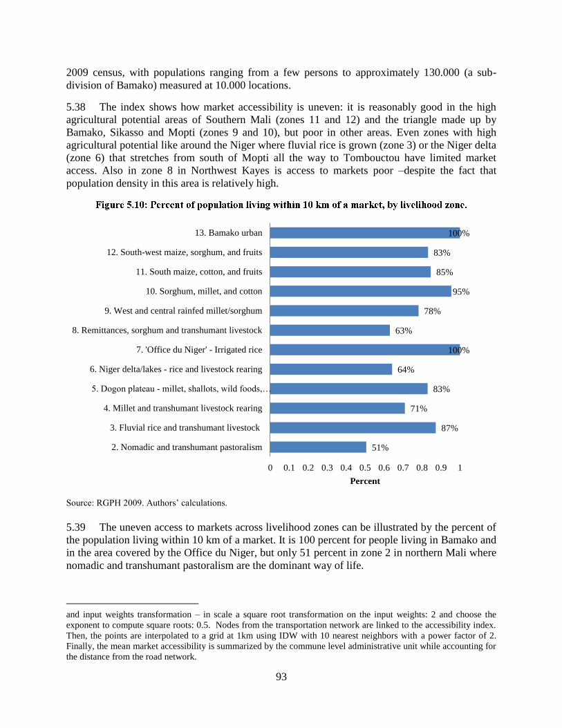
93
2009 census, with populations ranging from a few persons to approximately 130.000 (a sub-
division of Bamako) measured at 10.000 locations.
5.38 The index shows how market accessibility is uneven: it is reasonably good in the high
agricultural potential areas of Southern Mali (zones 11 and 12) and the triangle made up by
Bamako, Sikasso and Mopti (zones 9 and 10), but poor in other areas. Even zones with high
agricultural potential like around the Niger where fluvial rice is grown (zone 3) or the Niger delta
(zone 6) that stretches from south of Mopti all the way to Tombouctou have limited market
access. Also in zone 8 in Northwest Kayes is access to markets poor –despite the fact that
population density in this area is relatively high.
Source: RGPH 2009. Authors’ calculations.
5.39 The uneven access to markets across livelihood zones can be illustrated by the percent of
the population living within 10 km of a market. It is 100 percent for people living in Bamako and
in the area covered by the Office du Niger, but only 51 percent in zone 2 in northern Mali where
nomadic and transhumant pastoralism are the dominant way of life.
and input weights transformation – in scale a square root transformation on the input weights: 2 and choose the
exponent to compute square roots: 0.5. Nodes from the transportation network are linked to the accessibility index.
Then, the points are interpolated to a grid at 1km using IDW with 10 nearest neighbors with a power factor of 2.
Finally, the mean market accessibility is summarized by the commune level administrative unit while accounting for
the distance from the road network.
51%
87%
71%
83%
64%
100%
63%
78%
95%
85%
83%
100%
0 0.1 0.2 0.3 0.4 0.5 0.6 0.7 0.8 0.9 1
2. Nomadic and transhumant pastoralism
3. Fluvial rice and transhumant livestock
4. Millet and transhumant livestock rearing
5. Dogon plateau - millet, shallots, wild foods,…
6. Niger delta/lakes - rice and livestock rearing
7. 'Office du Niger' - Irrigated rice
8. Remittances, sorghum and transhumant livestock
9. West and central rainfed millet/sorghum
10. Sorghum, millet, and cotton
11. South maize, cotton, and fruits
12. South-west maize, sorghum, and fruits
13. Bamako urban
Percent
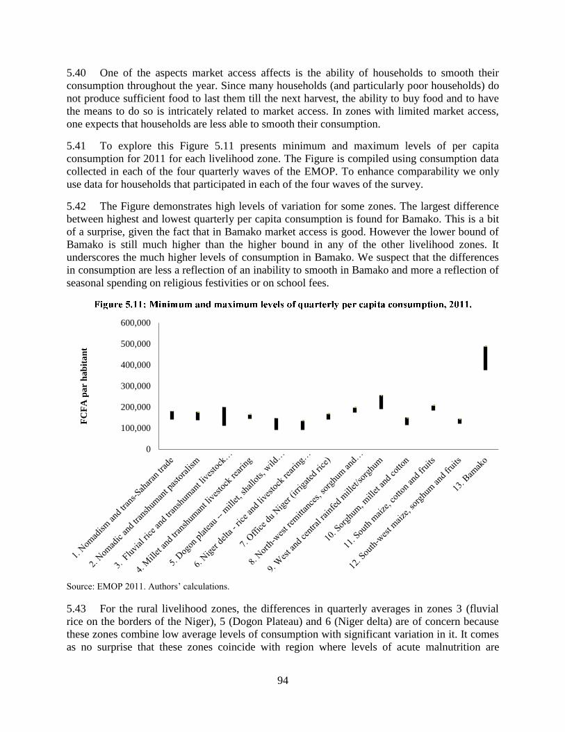
94
5.40 One of the aspects market access affects is the ability of households to smooth their
consumption throughout the year. Since many households (and particularly poor households) do
not produce sufficient food to last them till the next harvest, the ability to buy food and to have
the means to do so is intricately related to market access. In zones with limited market access,
one expects that households are less able to smooth their consumption.
5.41 To explore this Figure 5.11 presents minimum and maximum levels of per capita
consumption for 2011 for each livelihood zone. The Figure is compiled using consumption data
collected in each of the four quarterly waves of the EMOP. To enhance comparability we only
use data for households that participated in each of the four waves of the survey.
5.42 The Figure demonstrates high levels of variation for some zones. The largest difference
between highest and lowest quarterly per capita consumption is found for Bamako. This is a bit
of a surprise, given the fact that in Bamako market access is good. However the lower bound of
Bamako is still much higher than the higher bound in any of the other livelihood zones. It
underscores the much higher levels of consumption in Bamako. We suspect that the differences
in consumption are less a reflection of an inability to smooth in Bamako and more a reflection of
seasonal spending on religious festivities or on school fees.
Source: EMOP 2011. Authors’ calculations.
5.43 For the rural livelihood zones, the differences in quarterly averages in zones 3 (fluvial
rice on the borders of the Niger), 5 (Dogon Plateau) and 6 (Niger delta) are of concern because
these zones combine low average levels of consumption with significant variation in it. It comes
as no surprise that these zones coincide with region where levels of acute malnutrition are
0
100,000
200,000
300,000
400,000
500,000
600,000
FC
FA
pa
r h
ab
ita
nt

95
highest (Tombouctou, Figure 3.20). In zones 4 (millet and transhumant livestock rearing), 11 and
12 (South and South West) the variation in quarterly consumption is low, suggesting that
household are able to smooth their consumption throughout the year. We thus find a close
association between market access and food (in) security.
5.44 Much as the incidence of access to markets is informative and the association between
lack of access and acute malnutrition of concern, decisions about fixed investments such as roads
not only have to be informed by need but also by the number of people that are reached and their
economic potential. To assess this, we repeat Figure 5.9 but now show the number of households
within each livelihood zone that do not live within 10km of a road. This is presented in Figure
5.12, which suggests that despite relatively high access incidence rates of respectively 78 percent
and 85 percent, additional infrastructure in zones 9 and 11 could connect more than 1.2 million
people to markets. In combination with the relatively high agro-ecological potential of these
zones, it suggests an investment strategy that considers these two zones, but also the Niger delta
where not only the average access rate is poor, but the agro-ecological potential high and the
number of people that can be reached substantial.
Source: RGPH 2009. Authors’ calculations.
5.45 Accessibility is more than new road construction alone. Limited road maintenance
renders many roads unusable especially during the rainy season: rural roads, the pistes
améliorées, are in a poor state: only 5 percent are in a good condition and as many as 47 percent
are listed as being in a poor condition (Table 5.4).
0 200,000 400,000 600,000 800,000
2. Nomadic and transhumant pastoralism
3. Fluvial rice and transhumant livestock
4. Millet and transhumant livestock rearing
5. Dogon plateau - millet, shallots, wild foods,…
6. Niger delta/lakes - rice and livestock rearing
7. 'Office du Niger' - Irrigated rice
8. Remittances, sorghum and transhumant…
9. West and central rainfed millet/sorghum
10. Sorghum, millet, and cotton
11. South maize, cotton, and fruits
12. South-west maize, sorghum, and fruits
13. Bamako urban
Number of people without access
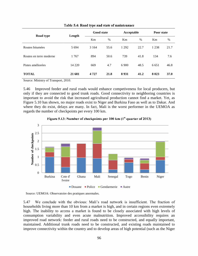
96
Road type Length Good state Acceptable Poor state
Km % Km % Km %
Routes bitumées 5 694 3 164 55.6 1 292 22.7 1 238 21.7
Routes en terre moderne 1 767 894 50.6 739 41.8 134 7.6
Pistes améliorées 14 220 669 4.7 6 900 48.5 6 651 46.8
TOTAL 21 681 4 727 21.8 8 931 41.2 8 023 37.0
Source: Ministry of Transport, 2010.
5.46 Improved feeder and rural roads would enhance competiveness for local producers, but
only if they are connected to good trunk roads. Good connectivity to neighboring countries is
important to avoid the risk that increased agricultural production cannot find a market. Yet, as
Figure 5.10 has shown, no major roads exist to Niger and Burkina Faso as well as to Dakar. And
where they do exist, delays are many. In fact, Mali is the worst performer in the UEMOA as
regards the number of checkpoints per every 100 km.
Source: UEMOA: Observatoire des pratiques anormales.
5.47 We conclude with the obvious: Mali’s road network is insufficient. The fraction of
households living more than 10 km from a market is high, and in certain regions even extremely
high. The inability to access a market is found to be closely associated with high levels of
consumption variability and even acute malnutrition. Improved accessibility requires an
improved road network: feeder and rural roads need to be constructed, and equally important,
maintained. Additional trunk roads need to be constructed, and existing roads maintained to
improve connectivity within the country and to develop areas of high potential (such as the Niger
0
0.5
1
1.5
2
2.5
3
Burkina Cote d'
Ivoire
Ghana Mali Senegal Togo Benin Niger
Nu
mb
er o
f ch
eck
po
ints
Douane Police Gendarmerie Autre

97
delta) to major markets. International connectivity (Bamako-Dakar, Bamako-Niger and Bamako-
Burkina Faso) also needs to be improved. Connections to other countries in the Sahel need to
improve particularly to support a poverty reduction strategy poised towards an increased
production of food crops. Without access to international markets a strategy that has brought
impressive results in the years 2000 may not be sustained, particularly when the domestic
demand for these crops become saturated.
5.48 High (fixed and other) costs and limited budgets create difficult choices for the provision
of public services. Trade-offs have to be made between giving as many as possible access (i.e.
offering the service where the cost per beneficiary is lowest) and ensuring that everybody has the
same opportunity to access a service (comparable access rates across space irrespective of the
cost of provision). This chapter noted how, in reality, the discussion is more complex than this
simple dichotomy. Quality matters as do complementary measures such as an adequate road
maintenance budget and policies to prevent unnecessary checkpoints.
5.49 The chapter illustrated how secondary schools could only be provided in a cost-efficient
manner in a limited fraction of all communities, which is unacceptable from an equity
perspective. Yet additional budget is unlikely to solve the problem, as the education system
would become prohibitively expensive, implying cuts in spending in other, equally important
sectors. So there is much pressure to deliver existing services to more people at lower cost.
5.50 The issue of high unit cost limiting the degree to which services can be provided exists
across the globe, but is particularly pressing in a low population density environment like in Mali
where the fixed cost of service provision can only be shared between relatively few beneficiaries.
Finding solutions to the challenge of high unit costs is, therefore, critical.
5.51 There are various ways to deal with these challenges. One is efficiency. Wastage is never
acceptable and it is critical that the public sector is vigilant about the unit cost at which various
services are provided in different locations.55 Good planning is essential to avoiding wastage:
constructing roads in the absence of means to maintain them amounts to waste that could easily
be avoided; high drop-out rates in primary school is equally wasteful.
5.52 Another way to address the “how to provide services in a cost-effective manner in a low
density environment challenge” is by embracing migration. In chapter two it was suggested that
pull factors –particularly better access to services and economic opportunities are amongst the
reasons for migration. Temporary labor migration as well as permanent migration are already
common, and moving people to the service rather than the service to the people deserves to be
embraced as a cost-effective way of dealing with low-density problems. Policies need to
facilitate internal migration by reducing its cost and increasing the probability of success.
Secondary schools or hospitals could offer boarding facilities. Pastoralists may be asked to travel
with their animals to veterinary services; businesses can be facilitated to move to towns where
electricity is can be offered. Improved education would increase the success rate of migration as
unskilled migrants are found to be least likely to succeed.
55
It is beyond the scope of this document to do so, but it is clear that the analysis that was prepared about the
distribution of primary and secondary schools could be complemented with an analysis of the unit cost of
investment.
98
5.53 A third way to reduce the unit cost of service delivery is by embracing innovation. The
challenge posed by low population density is so pressing that reducing the cost of service
provision through innovation deserves to be embraced as a core objective of public policy. There
are many ways to do so, some of which are already implemented as a matter of routine. Wells
and dirt roads are constructed in areas where population density is low; piped water and
tarmacked roads are available in cities where population density is high. Other approaches are
un-tried: in low density areas students of different grades could share classrooms and teachers;
secondary school teachers could be required to teach multiple subjects; veterinary and
vaccination services could be offered in an integrated manner.
5.54 With the advent of new technologies, new opportunities to reduce the unit cost of service
provision abound. Mobile phone technology allows offering a plethora of services from voice
calls to internet access to mobile money transfers and banking and can do so without the need to
invest in an expensive cable network. The implications of this for poor households living in
isolated areas are far-reaching. Compare for instance the limited availability of financial services
as presently offered by savings banks (Figure 5.14) with what would be feasible if mobile money
transfers, mobile savings and even full fletched banking services were available as they are in
Kenya, Uganda or Tanzania.
5.55 The options are not limited to mobile phone technology. In the chapter we discussed how
advances in solar technology makes it affordable to offer lighting and cell phone charging
services to all. Cheap tablet computers offer new –cheaper and faster- opportunities for data
collection; cheap motor bikes allow households to deal with poor rural roads and have made the
market for transport services more competitive.
5.56 Government can nurture innovations. In some cases (motor bikes for instance)
Government needs to do very little as the market is already taking care of it. In other instances
(mobile telephony) Government will need to provide the appropriate regulatory framework to
ensure that competition is increased such that the benefits of mobile telephony become available
to many. Vigilance is needed to avoid policies which go contrary to the objective of access for
all. The mandatory registration of SIM cards which is being considered is an illustration of a
policy that – if implemented, would yield little in benefits, but which would make it much harder
for those who need the service most, people living isolated in low density areas, to benefit from
mobile phone services.
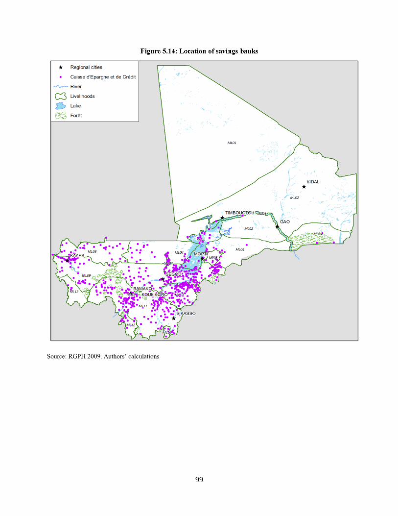
99
Source: RGPH 2009. Authors’ calculations
100
Poverty Reduction and Growth in the Face of
Spatial Challenges
6.1 One importance of physical distance to the world’s markets was illustrated by the night-
time lights map presented in the introduction. In this chapter we explore the connection between
poverty reduction and growth and conclude that Mali is well poised to rapidly reduce poverty,
provided growth is accelerated. The required growth acceleration falls within the realm of the
feasible. The chapter then considers how, in the face of spatial constraints, such an acceleration
might be brought about.
6.2 At an average rate of 1.5 percent per capita since 2000, growth has been lackluster. The
main reason why poverty declined between 2001 and 2010 is because of the decline in
inequality56
as a consequence of the fact that consumption of the poorest segments of the
population increased, while consumption of the wealthiest declined. As a consequence of this
redistribution the Gini coefficient for Mali dropped from 0.40 in 2001 to around 0.33 in 2010.
6.3 Looking to the future it is relevant to know what the rate of growth would have to be to
half poverty by, say, 2030. This is an ambitious objective as it implies that poverty would reduce
to around 20 percent, but it is significantly less ambitious than the World Bank’s objective of 3
percent poverty by 2030.
6.4 To prepare poverty projections, assumptions have to be made about future changes in
inequality, the relation between GDP growth and consumption growth and the rate of population
increase. With respect to inequality we make the simplifying assumption that inequality will not
change. In other words, it is hypothesized that the shape of the consumption distribution will
remain unchanged implying that poverty reduction will not come from changes in inequality but
from consumption growth which benefits all households equally. The reason to assume this –in
spite of the fact that in the recent past inequality reduction was the main driver of poverty
reduction is that, while future decreases in inequality cannot be ruled out, already the level of
inequality in Mali is the lowest in the region (Figure 6.1). Further decreases in inequality can be
expected to be increasingly difficult to realize.
56
A decomposition of the change in poverty between 2001 and 2010 shows that of the decline of 9.8 percentage
points, 1 percentage point can be attributed to growth and 8 to a change in inequality. The remainder is attributable
to the interaction between both effects.
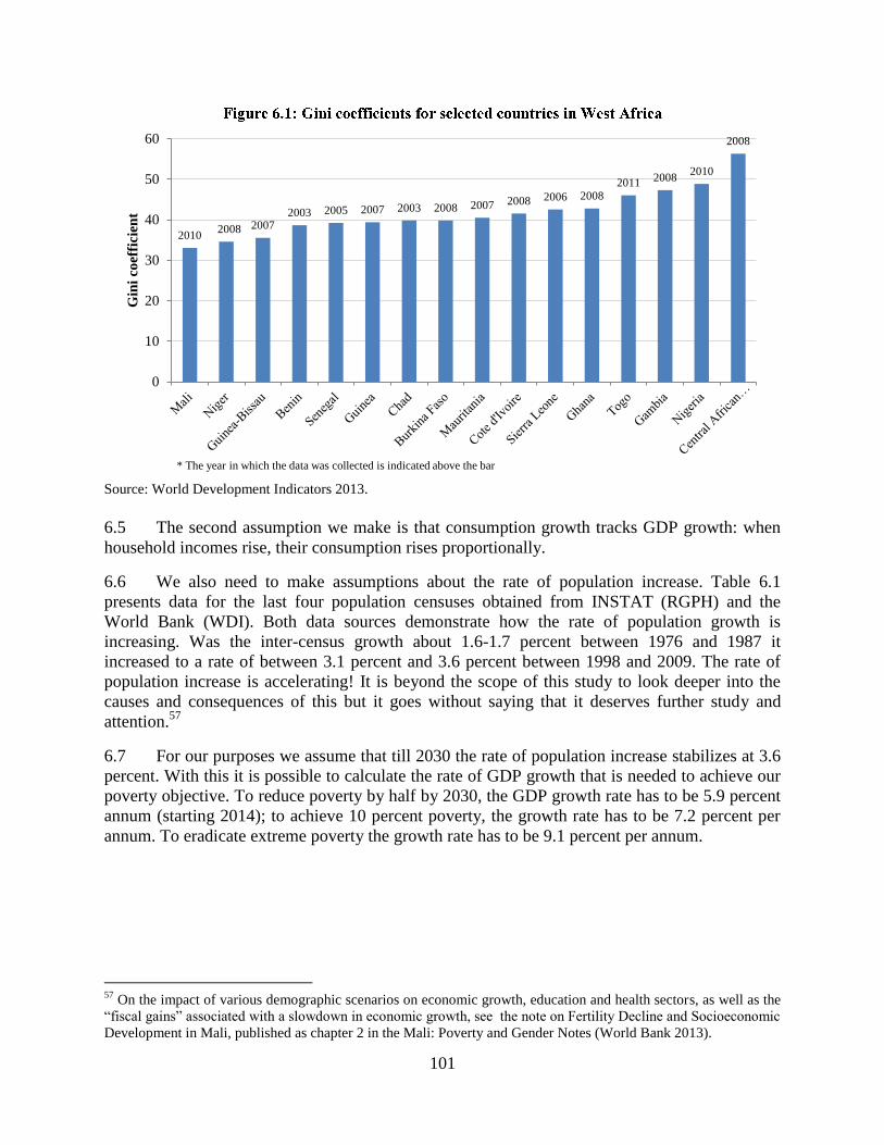
101
Source: World Development Indicators 2013.
6.5 The second assumption we make is that consumption growth tracks GDP growth: when
household incomes rise, their consumption rises proportionally.
6.6 We also need to make assumptions about the rate of population increase. Table 6.1
presents data for the last four population censuses obtained from INSTAT (RGPH) and the
World Bank (WDI). Both data sources demonstrate how the rate of population growth is
increasing. Was the inter-census growth about 1.6-1.7 percent between 1976 and 1987 it
increased to a rate of between 3.1 percent and 3.6 percent between 1998 and 2009. The rate of
population increase is accelerating! It is beyond the scope of this study to look deeper into the
causes and consequences of this but it goes without saying that it deserves further study and
attention.57
6.7 For our purposes we assume that till 2030 the rate of population increase stabilizes at 3.6
percent. With this it is possible to calculate the rate of GDP growth that is needed to achieve our
poverty objective. To reduce poverty by half by 2030, the GDP growth rate has to be 5.9 percent
annum (starting 2014); to achieve 10 percent poverty, the growth rate has to be 7.2 percent per
annum. To eradicate extreme poverty the growth rate has to be 9.1 percent per annum.
57
On the impact of various demographic scenarios on economic growth, education and health sectors, as well as the
“fiscal gains” associated with a slowdown in economic growth, see the note on Fertility Decline and Socioeconomic
Development in Mali, published as chapter 2 in the Mali: Poverty and Gender Notes (World Bank 2013).
2010 2008 2007
2003 2005 2007 2003 2008 2007 2008 2006 2008 2011 2008
2010
2008
0
10
20
30
40
50
60G
ini
coef
fici
ent
* The year in which the data was collected is indicated above the bar
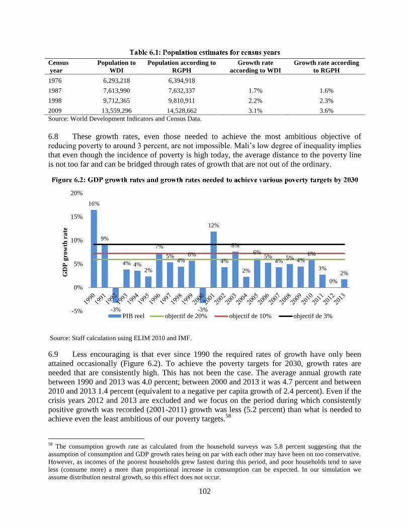
102
Census
year
Population to
WDI
Population according to
RGPH
Growth rate
according to WDI
Growth rate according
to RGPH
1976 6,293,218 6,394,918
1987 7,613,990 7,632,337 1.7% 1.6%
1998 9,712,365 9,810,911 2.2% 2.3%
2009 13,559,296 14,528,662 3.1% 3.6%
Source: World Development Indicators and Census Data.
6.8 These growth rates, even those needed to achieve the most ambitious objective of
reducing poverty to around 3 percent, are not impossible. Mali’s low degree of inequality implies
that even though the incidence of poverty is high today, the average distance to the poverty line
is not too far and can be bridged through rates of growth that are not out of the ordinary.
Source: Staff calculation using ELIM 2010 and IMF.
6.9 Less encouraging is that ever since 1990 the required rates of growth have only been
attained occasionally (Figure 6.2). To achieve the poverty targets for 2030, growth rates are
needed that are consistently high. This has not been the case. The average annual growth rate
between 1990 and 2013 was 4.0 percent; between 2000 and 2013 it was 4.7 percent and between
2010 and 2013 1.4 percent (equivalent to a negative per capita growth of 2.4 percent). Even if the
crisis years 2012 and 2013 are excluded and we focus on the period during which consistently
positive growth was recorded (2001-2011) growth was less (5.2 percent) than what is needed to
achieve even the least ambitious of our poverty targets.58
58
The consumption growth rate as calculated from the household surveys was 5.8 percent suggesting that the
assumption of consumption and GDP growth rates being on par with each other may have been on too conservative.
However, as incomes of the poorest households grew fastest during this period, and poor households tend to save
less (consume more) a more than proportional increase in consumption can be expected. In our simulation we
assume distribution neutral growth, so this effect does not occur.
16%
9%
-3%
4% 4% 2%
7%
5% 4%
6%
-3%
12%
4%
8%
2%
6% 5%
4% 5% 4%
6%
3%
0%
2%
-5%
0%
5%
10%
15%
20%
GD
P g
row
th r
ate
PIB reel objectif de 20% objectif de 10% objectif de 3%

103
6.10 One implication is that growth acceleration is needed. Doing so will require a serious
policy effort. Before saying more about what would be needed to accelerate growth, another
implication is equally important: it is critical that the low rates of inequality are maintained either
by ensuring that growth remains broadly shared, or through redistributive measures. Particularly
when more is being earned from natural resources, redistribution measures may have to be
considered.
6.11 As an aside, poverty can also be reduced through transfers. These can be in kind (skill
training) or in cash offered by a social safety net. Social safety nets can be used as short term
instruments to help the poor cope with economic shocks, but also as medium/long-term poverty
alleviation programs, supporting minimum consumption levels and promoting the accumulation
of human and physical capital. When cash transfers are provided over multiple periods to poor
households, it is typically first used it to pay off debts and later to accumulate productive assets
or to buy inputs (fertilizer). 59
This enhances productive capacity and resilience such that
eventually they no longer require support. Experience shows that these objectives are more
effectively achieved when safety net support is combined with investments in livelihoods.60
Adaptive social protection is one of the tools to be used. It enables beneficiaries to invest in
productive assets, stimulates use of basic social services and reduces sensitivity to future shocks
6.12 The combination on income growth with transfers has the potential to reduce poverty
rapidly in Mali. Expanding the simulations presented above by including a (perfectly targeted)
transfer equivalent of 2 percent of GDP shows that is feasible to reduce poverty to 3 percent by
2030 as long as the consumption growth amongst the poorest households is 2 percent per capita.
6.13 Between 2000 and 2010, GDP per capita grew steadily, before much of the gains were
lost as a result of the combined effects of poor rains and the crisis in the north. By 2013, GDP
per capita was at the same level as it was in 2007-8 (Table 7.1). GDP growth has been driven by
the primary and tertiary sectors, largely gold, cotton, cereals and aid while the secondary sector
stagnated. Growth in the primary sector was driven by agriculture and within agriculture by food
crops (57 percent of total agricultural production) and rice (28 percent of total agricultural GDP).
Industrial crops, and cotton only play a limited role within the agricultural sector (both contribute
8 percent to agricultural GDP). Within the primary sector, livestock rearing is important but the
sector has not grown much since 2010. It makes up about a quarter of primary sector GDP.
59 See for instance for evidence from Niger: Quentin Stoeffler and Bradford Mills (2014): Households’ investments
in durable and productive assets in Niger: quasi-experimental evidences from a cash transfer project. 60
Even so, for some households, depending on the context, this process can take a long time.

104
Source: calculated from IMF 2014.
6.14 In the tertiary sector growth was driven by trade, transport and telecom and fuelled in part
by large private investments in the mining sector which led to large increases in the volume of
trade (total imports quadrupled between 2001 and 2013 from CFAF 600 billion to over CFAF
2,500 billion). The high level of investments by the private sector is matched by significant
public sector investments which comprised a significant part of the budget. Of concern are the
large fluctuations in public investment spending – which hamper efficient planning and
execution, and the fact that the level of public investments declined significantly during the crisis
(Figure 6.4).
Source: IMF 2014.
0
20
40
60
80
100
120
2000 2001 2002 2003 2004 2005 2006 2007 2008 2009 2010 2011 2012 2013
GD
P p
er c
ap
ita
('0
00
FC
FA
)
BIP Secteur primaire Secteur secondaire Secteur tertiare
0.0
5.0
10.0
15.0
20.0
25.0
30.0
35.0
2000 2001 2002 2003 2004 2005 2006 2007 2008 2008 2009 2009 2010 2011 2012 2013
Per
cen
t o
f G
DP
Secteur public Secteur prive

105
6.15 The lack of growth in the secondary sector was flagged in chapter two when it was found
that despite rapid urbanization Bamako is not a driver of growth. Possibly with the exception of
New Zealand there are no countries that have reached middle income status without going
through a phase of industrialization. Particularly as the scope for increased mineral production or
for increased aid (another important driver of consumption and investment) is limited –at least as
long as the north remains insecure, and as domestic demand is limited, growth will need to come
from factors that combine Mali’s comparative advantages in the primary sector, with industrial
processing and exports.
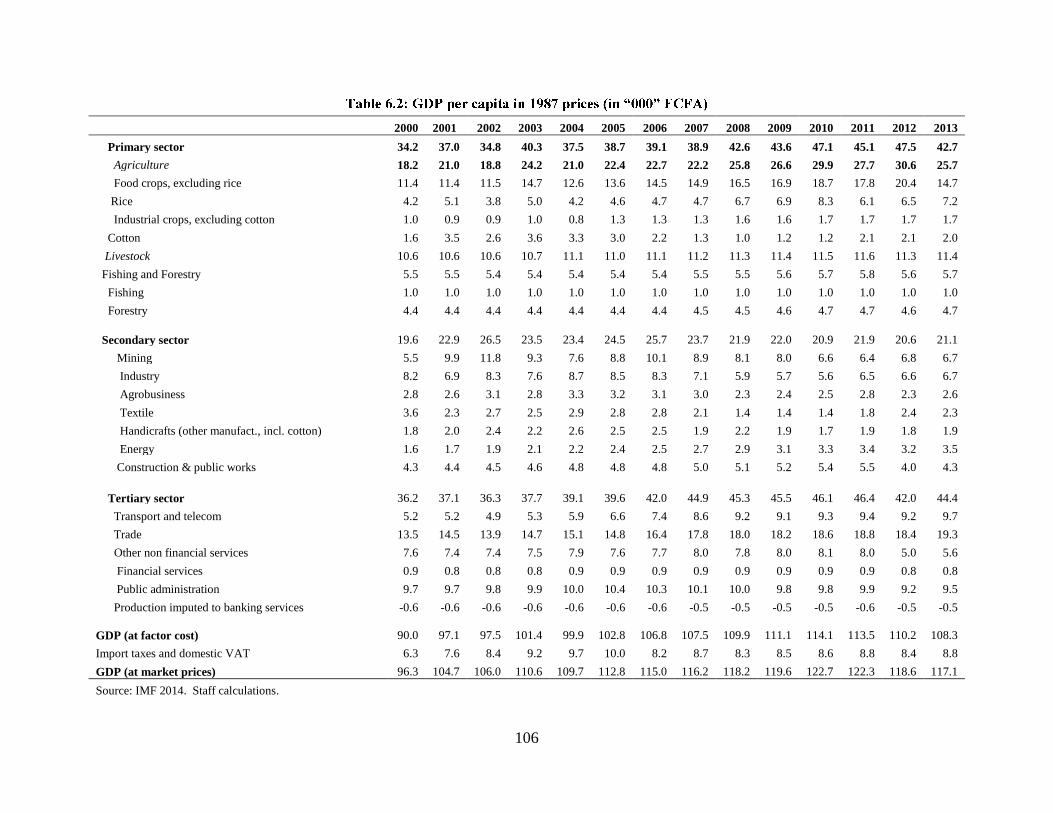
106
2000 2001 2002 2003 2004 2005 2006 2007 2008 2009 2010 2011 2012 2013
Primary sector 34.2 37.0 34.8 40.3 37.5 38.7 39.1 38.9 42.6 43.6 47.1 45.1 47.5 42.7
Agriculture 18.2 21.0 18.8 24.2 21.0 22.4 22.7 22.2 25.8 26.6 29.9 27.7 30.6 25.7
Food crops, excluding rice 11.4 11.4 11.5 14.7 12.6 13.6 14.5 14.9 16.5 16.9 18.7 17.8 20.4 14.7
Rice 4.2 5.1 3.8 5.0 4.2 4.6 4.7 4.7 6.7 6.9 8.3 6.1 6.5 7.2
Industrial crops, excluding cotton 1.0 0.9 0.9 1.0 0.8 1.3 1.3 1.3 1.6 1.6 1.7 1.7 1.7 1.7
Cotton 1.6 3.5 2.6 3.6 3.3 3.0 2.2 1.3 1.0 1.2 1.2 2.1 2.1 2.0
Livestock 10.6 10.6 10.6 10.7 11.1 11.0 11.1 11.2 11.3 11.4 11.5 11.6 11.3 11.4
Fishing and Forestry 5.5 5.5 5.4 5.4 5.4 5.4 5.4 5.5 5.5 5.6 5.7 5.8 5.6 5.7
Fishing 1.0 1.0 1.0 1.0 1.0 1.0 1.0 1.0 1.0 1.0 1.0 1.0 1.0 1.0
Forestry 4.4 4.4 4.4 4.4 4.4 4.4 4.4 4.5 4.5 4.6 4.7 4.7 4.6 4.7
Secondary sector 19.6 22.9 26.5 23.5 23.4 24.5 25.7 23.7 21.9 22.0 20.9 21.9 20.6 21.1
Mining 5.5 9.9 11.8 9.3 7.6 8.8 10.1 8.9 8.1 8.0 6.6 6.4 6.8 6.7
Industry 8.2 6.9 8.3 7.6 8.7 8.5 8.3 7.1 5.9 5.7 5.6 6.5 6.6 6.7
Agrobusiness 2.8 2.6 3.1 2.8 3.3 3.2 3.1 3.0 2.3 2.4 2.5 2.8 2.3 2.6
Textile 3.6 2.3 2.7 2.5 2.9 2.8 2.8 2.1 1.4 1.4 1.4 1.8 2.4 2.3
Handicrafts (other manufact., incl. cotton) 1.8 2.0 2.4 2.2 2.6 2.5 2.5 1.9 2.2 1.9 1.7 1.9 1.8 1.9
Energy 1.6 1.7 1.9 2.1 2.2 2.4 2.5 2.7 2.9 3.1 3.3 3.4 3.2 3.5
Construction & public works 4.3 4.4 4.5 4.6 4.8 4.8 4.8 5.0 5.1 5.2 5.4 5.5 4.0 4.3
Tertiary sector 36.2 37.1 36.3 37.7 39.1 39.6 42.0 44.9 45.3 45.5 46.1 46.4 42.0 44.4
Transport and telecom 5.2 5.2 4.9 5.3 5.9 6.6 7.4 8.6 9.2 9.1 9.3 9.4 9.2 9.7
Trade 13.5 14.5 13.9 14.7 15.1 14.8 16.4 17.8 18.0 18.2 18.6 18.8 18.4 19.3
Other non financial services 7.6 7.4 7.4 7.5 7.9 7.6 7.7 8.0 7.8 8.0 8.1 8.0 5.0 5.6
Financial services 0.9 0.8 0.8 0.8 0.9 0.9 0.9 0.9 0.9 0.9 0.9 0.9 0.8 0.8
Public administration 9.7 9.7 9.8 9.9 10.0 10.4 10.3 10.1 10.0 9.8 9.8 9.9 9.2 9.5
Production imputed to banking services -0.6 -0.6 -0.6 -0.6 -0.6 -0.6 -0.6 -0.5 -0.5 -0.5 -0.5 -0.6 -0.5 -0.5
GDP (at factor cost) 90.0 97.1 97.5 101.4 99.9 102.8 106.8 107.5 109.9 111.1 114.1 113.5 110.2 108.3
Import taxes and domestic VAT 6.3 7.6 8.4 9.2 9.7 10.0 8.2 8.7 8.3 8.5 8.6 8.8 8.4 8.8
GDP (at market prices) 96.3 104.7 106.0 110.6 109.7 112.8 115.0 116.2 118.2 119.6 122.7 122.3 118.6 117.1
Source: IMF 2014. Staff calculations.
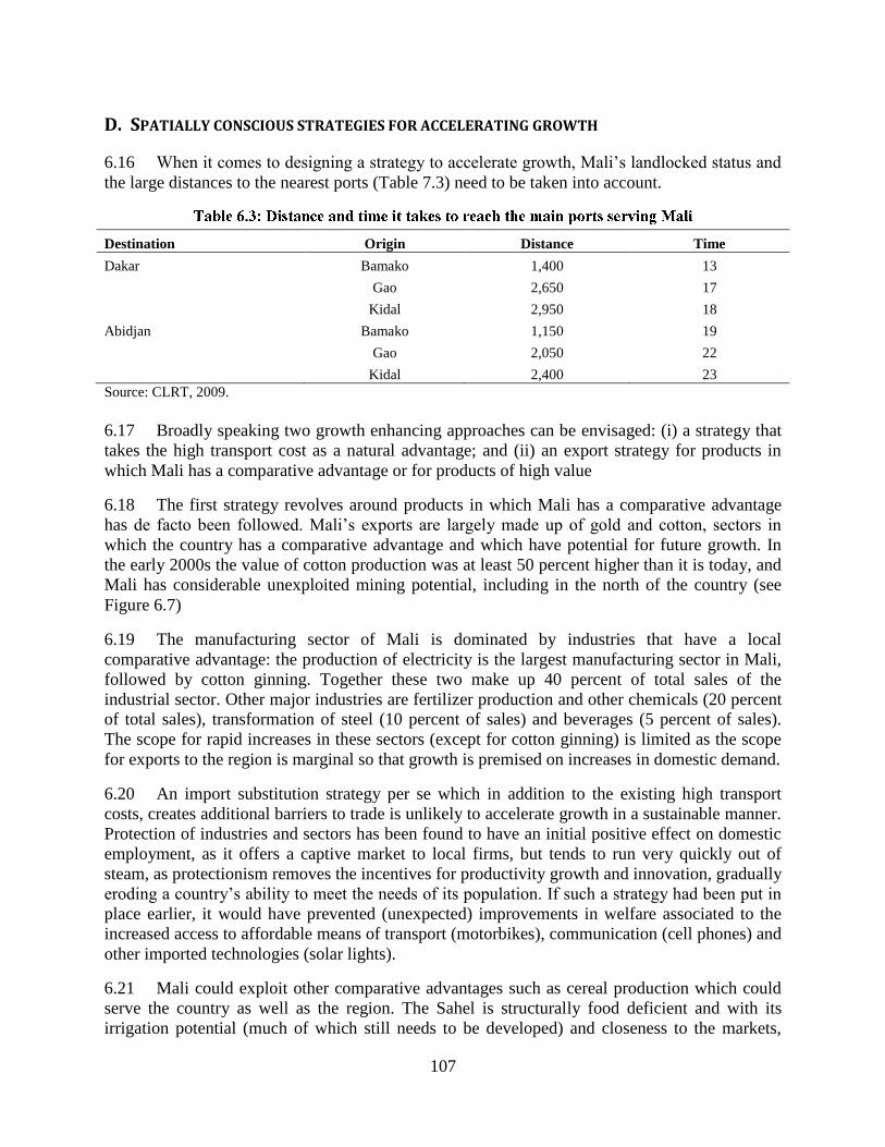
107
D. SPATIALLY CONSCIOUS STRATEGIES FOR ACCELERATING GROWTH
6.16 When it comes to designing a strategy to accelerate growth, Mali’s landlocked status and
the large distances to the nearest ports (Table 7.3) need to be taken into account.
Destination Origin Distance Time
Dakar Bamako 1,400 13
Gao 2,650 17
Kidal 2,950 18
Abidjan Bamako 1,150 19
Gao 2,050 22
Kidal 2,400 23
Source: CLRT, 2009.
6.17 Broadly speaking two growth enhancing approaches can be envisaged: (i) a strategy that
takes the high transport cost as a natural advantage; and (ii) an export strategy for products in
which Mali has a comparative advantage or for products of high value
6.18 The first strategy revolves around products in which Mali has a comparative advantage
has de facto been followed. Mali’s exports are largely made up of gold and cotton, sectors in
which the country has a comparative advantage and which have potential for future growth. In
the early 2000s the value of cotton production was at least 50 percent higher than it is today, and
Mali has considerable unexploited mining potential, including in the north of the country (see
Figure 6.7)
6.19 The manufacturing sector of Mali is dominated by industries that have a local
comparative advantage: the production of electricity is the largest manufacturing sector in Mali,
followed by cotton ginning. Together these two make up 40 percent of total sales of the
industrial sector. Other major industries are fertilizer production and other chemicals (20 percent
of total sales), transformation of steel (10 percent of sales) and beverages (5 percent of sales).
The scope for rapid increases in these sectors (except for cotton ginning) is limited as the scope
for exports to the region is marginal so that growth is premised on increases in domestic demand.
6.20 An import substitution strategy per se which in addition to the existing high transport
costs, creates additional barriers to trade is unlikely to accelerate growth in a sustainable manner.
Protection of industries and sectors has been found to have an initial positive effect on domestic
employment, as it offers a captive market to local firms, but tends to run very quickly out of
steam, as protectionism removes the incentives for productivity growth and innovation, gradually
eroding a country’s ability to meet the needs of its population. If such a strategy had been put in
place earlier, it would have prevented (unexpected) improvements in welfare associated to the
increased access to affordable means of transport (motorbikes), communication (cell phones) and
other imported technologies (solar lights).
6.21 Mali could exploit other comparative advantages such as cereal production which could
serve the country as well as the region. The Sahel is structurally food deficient and with its
irrigation potential (much of which still needs to be developed) and closeness to the markets,

108
Mali is a well placed to serve other landlocked countries with maize, rice and other cereals. A
strategy that focuses on increased maize, rice and other cereal production also has immediate
benefits for Mali’s food security, and as we have seen in Chapter 4 was one of the reasons
behind the rapid reduction in poverty.
Source: World Bank, World Development Indicators 2013.
6.22 An agricultural growth strategy will only be viable in the long run if the country can to
tap into the demand originating from the region. Even then, the regional market for cereals is tiny
compared to the huge OECD market. For goods to reach this market they either need to be
profitably shipped by airplane (Paris is only 5 hours away) implying that they need to be (i) of
high value per unit of volume (cut flowers, dried mangos, horticultural products) or they need to
be (ii) goods for which Mali experiences a large favorable productivity differential with the rest
of the world like leather and leather products. Instead of physically transporting goods (iii)
services could also be traded through IT technology. Bamako is the music capital of West Africa,
and Mali’s colorful crafts and leather work are appreciated across the globe. Migration and
tourism (iv) present yet another approach to exporting services. One of the zones with the highest
rate of consumption growth is in north Kayes (zone 8) in which international migration is a
dominant (and successful) livelihood strategy.
6.23 This second approach which combines structural-transformation with exports will take a
long gestation period, and requires a consistent, multi-faceted and active government
involvement to facilitate coordination in the sector, to address information externalities and to
reduce high levels of transaction costs. It can be done: Ethiopia, Kenya and Tanzania have
successfully entered the cut flower industry, and Ethiopia has successfully developed its leather
industry. However such a strategy requires considerable demands on Government capacity, and a
long term vision, to be successful (see box 6.1).
While many agree that the private sector is a driver of growth, there appears to have been little consensus on
governments’ ability to push the private sector to promoting growth and development; let alone on whether such
interventions are necessary for industrial take-off. With the right polices, governments in poor countries can
systematically improve the welfare of their society through technological catch up and industrial upgrading. Given
2,740 2,740 2,740 2,962 3,015 3,127 3,127 3,127
4,405
1,720 1,720 1,720 1,920 1,940 1,940
1,740 1,740 1,740
-
500
1,000
1,500
2,000
2,500
3,000
3,500
4,000
4,500
5,000
2005 2006 2007 2008 2009 2010 2011 2012 2013
Co
st t
o i
mp
ort
(U
S$
per
con
tain
er)
Mali Senegal Cote d'Ivoire

109
the ubiquity of market failures ranging from information externalities to high levels of transaction costs and co-
ordination problems, government intervention in the allocation of productive resources is often unavoidable, but
intervening successfully is demanding on government capacity and requires a long term vision.
The leather industry in Ethiopia can illustrate what an active industrial policy entails and what it can achieve. Like
Mali Ethiopia is endowed with the resource base required for the commercial production of leather and leather
products and like in Mali there is a history of leather processing in the country. Unlike Mali, Ethiopia also has a
history of shoe manufacturing that dates back to the 1920s. Ethiopia’s resources remained largely untapped due to a
host of reasons ranging from poor hides and skins collection to limited technology knowhow at the leather
processing phase.
The Ethiopian government employed multiple forms of industrial polices to reinvigorate the sector. In addition to
non-discriminatory general incentives that are available to all investors, several interventions were aimed at
upgrading the leather and leather products industry.
First the Ethiopian government helped organize six state-owned and two privately held companies to form the
Ethiopian Tanners Association, as a first step to properly organize the markets for semi-processed leather and leather
articles. The government also engaged in building the local production and marketing capacity through technology
learning from abroad. To his end a local institute, LLPTI, was selected to facilitate technology diffusion and upgrade
the skills of workers and managers in the industry and enterprises were encouraged enterprises to use foreign experts
by subsidizing the costs involved in their employment. The leather and leather goods industry had preferential
access to finance from the Development Bank of Ethiopia (DBE). The government also provided land and semi-
constructed factories to large and medium sized tanneries and footwear producers at highly discounted lease rates.
Finally, the government extensively used its tax and regulatory policies to encourage upgrading along the leather
value chain. The export
of raw hides and skins,
for example, became
banned to push local
processing of leather.
Similarly, the export of
semi-finished leather
products was subjected
to a 150% export tax in
2008. In 2012, the same
level of tax was imposed
on the export of crust
leather products. All
these interventions had
the combined effects of
improving value
addition, export and
employment in the
leather and leather
products industry (Figure B5.1).
Despite Ethiopia’s achievements there remains much room for improvements. Policies to improve facets of livestock
management and hide and skin collection would greatly improve raw hides and skins supply and quality for the
leather processing enterprises. Formal means of communication whereby all stakeholders are fairly represented
would facilitate dialogue and facilitate finding solutions to issues impacting the industry and would help build
greater trust among various stakeholders in the industry while enhancing the quality and ownership of regulations.
Source: Girum Abebe and Florian Schaefer (2013): High hopes and limited successes: experimenting with industrial
policies in the leather industry in Ethiopia. Authors’compilation.
6.24 Realizing Mali’s competitive potential requires addressing a number of cross-cutting
constraints, many of which have been identified before. A first element is to address high
transport and transit costs, both domestically, regionally and internationally. To stimulate trade
to OECD countries, and it addition to efforts to reduce transport costs to the ports of Dakar and
Figure B5.1: Export earnings in Ethiopia’s leather and leather products industry

110
Abidjan and to the Sahel it should be explored how Mali can become a regular (and cheap)
destination for cargo planes, or alternatively, whether cargo and passenger transport can be
combined efficiently.
6.25 Another cross cutting
factor is the need to exploit the
existing IT infrastructure. Mali has
a fiber-optic network which links
all major cities to the rest of the
world, and most citizens live
within reach of a mobile telephone
network. In combination this could
mean affordable internet access for
(almost) all, but it requires that the
right policies are put in place to
stimulate innovation and
competition. The present two
internet service providers and two
mobile telephone operators are
insufficient to induce the
competition needed to spur
innovation and price reductions.
International experience has shown
that the mobile telephony market is
most efficient and innovative when
a dominant party who is able to
innovate is challenged by 2 or 3
smaller and aggressive operators,
suggesting that additional telecom and ISP licenses would have to be issued.
6.26 A third cross cutting factor is the need to invest in human capital. This requires more than
improving the quality of primary and secondary education, but also that the right skills are
developed for international migrants to succeed or for entrepreneurs to benefit from the
opportunities offered by access to internet and the mobile phone network.
6.27 A final and critical cross cutting factor is peace and stability in the north. The
consequences of the continued crisis for economic growth are severe: resources which otherwise
could be used for developmental purposes (whether from donors or the Government) are being
re-allocated towards peace keeping efforts –viz. the decline in public investments. Meanwhile
international investors can be expected to shy away as long as security concerns remain –viz. the
increase in transport cost (Figure 6.5) and the decline in private investments. In the absence of
stability throughout the country sectors with growth potential like mining and tourism will
remain under-developed.
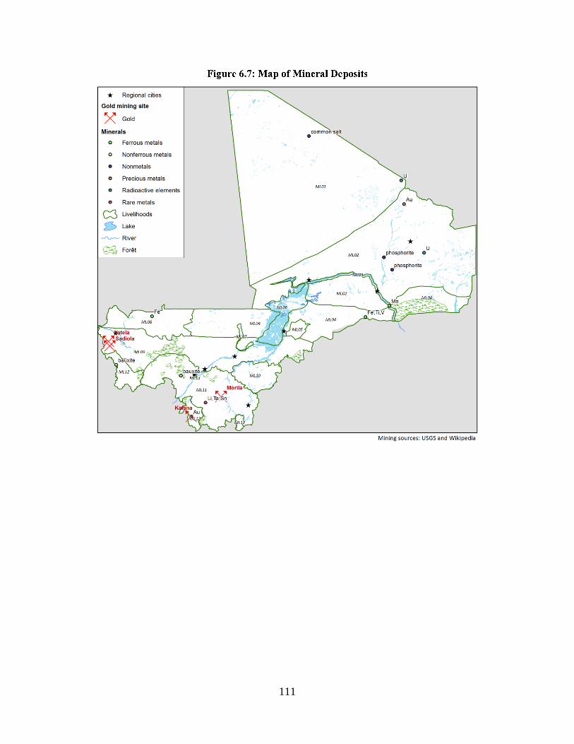
111
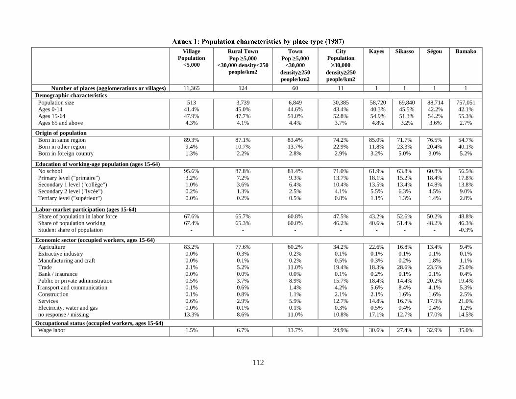
112
Village
Population
<5,000
Rural Town
Pop 5,000
<30,000 density<250
people/km2
Town
Pop 5,000
<30,000
density250
people/km2
City
Population
30,000
density250
people/km2
Kayes Sikasso Ségou Bamako
Number of places (agglomerations or villages) 11,365 124 60 11 1 1 1 1
Demographic characteristics
Population size
Ages 0-14
Ages 15-64
Ages 65 and above
513
41.4%
47.9%
4.3%
3,739
45.0%
47.7%
4.1%
6,849
44.6%
51.0%
4.4%
30,385
43.4%
52.8%
3.7%
58,720
40.3%
54.9%
4.8%
69,840
45.5%
51.3%
3.2%
88,714
42.2%
54.2%
3.6%
757,051
42.1%
55.3%
2.7%
Origin of population
Born in same region
Born in other region
Born in foreign country
89.3%
9.4%
1.3%
87.1%
10.7%
2.2%
83.4%
13.7%
2.8%
74.2%
22.9%
2.9%
85.0%
11.8%
3.2%
71.7%
23.3%
5.0%
76.5%
20.4%
3.0%
54.7%
40.1%
5.2%
Education of working-age population (ages 15-64)
No school
Primary level ("primaire")
Secondary 1 level ("collège")
Secondary 2 level ("lycée")
Tertiary level ("supérieur")
95.6%
3.2%
1.0%
0.2%
0.0%
87.8%
7.2%
3.6%
1.3%
0.2%
81.4%
9.3%
6.4%
2.5%
0.5%
71.0%
13.7%
10.4%
4.1%
0.8%
61.9%
18.1%
13.5%
5.5%
1.1%
63.8%
15.2%
13.4%
6.3%
1.3%
60.8%
18.4%
14.8%
4.5%
1.4%
56.5%
17.8%
13.8%
9.0%
2.8%
Labor-market participation (ages 15-64)
Share of population in labor force
Share of population working
Student share of population
67.6%
67.4%
-
65.7%
65.3%
-
60.8%
60.0%
-
47.5%
46.2%
-
43.2%
40.6%
-
52.6%
51.4%
-
50.2%
48.2%
-
48.8%
46.3%
-0.3%
Economic sector (occupied workers, ages 15-64)
Agriculture
Extractive industry
Manufacturing and craft
Trade
Bank / insurance
Public or private administration
Transport and communication
Construction
Services
Electricity, water and gas
no response / missing
83.2%
0.0%
0.0%
2.1%
0.0%
0.5%
0.1%
0.1%
0.6%
0.0%
13.3%
77.6%
0.3%
0.1%
5.2%
0.0%
3.7%
0.6%
0.8%
2.9%
0.1%
8.6%
60.2%
0.2%
0.2%
11.0%
0.0%
8.9%
1.4%
1.1%
5.9%
0.1%
11.0%
34.2%
0.1%
0.5%
19.4%
0.1%
15.7%
4.2%
2.1%
12.7%
0.3%
10.8%
22.6%
0.1%
0.3%
18.3%
0.2%
18.4%
5.6%
2.1%
14.8%
0.5%
17.1%
16.8%
0.1%
0.2%
28.6%
0.1%
14.4%
8.4%
1.6%
16.7%
0.4%
12.7%
13.4%
0.1%
1.8%
23.5%
0.1%
20.2%
4.1%
1.6%
17.9%
0.4%
17.0%
9.4%
0.1%
1.1%
25.0%
0.4%
19.4%
5.3%
2.5%
21.0%
1.2%
14.5%
Occupational status (occupied workers, ages 15-64)
Wage labor 1.5% 6.7% 13.7% 24.9% 30.6% 27.4% 32.9% 35.0%
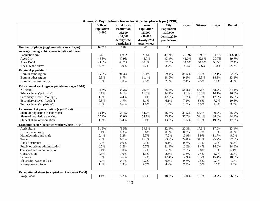
113
Annex 2: Population characteristics by place type (1998) Village
Population
<5,000
Rural Town
Population
5,000
<30,000
density<250
people/km2
Town
Population
5,000
<30,000
density250
people/km2
City
Population
30,000
density250
people/km2
Kayes Sikasso Ségou Bamako
Number of places (agglomerations or villages) 10,713 128 60 11 1 1 1 1
Average demographic characteristics of place
Population size
Ages 0-14
Ages 15-64
Ages 65 and above
646
46.8%
48.9%
4.3%
4,902
47.9%
48.2%
3.9%
7,564
45.7%
50.0%
4.2%
36,746
43.4%
52.9%
3.7%
71,897
41.0%
54.6%
4.4%
109,570
42.6%
54.8%
2.6%
91,882
39.7%
56.5%
3.8%
1,132,886
39.7%
57.4%
2.9%
Origin of population
Born in same region
Born in other region
Born in foreign country
96.7%
2.5%
0.8%
91.3%
6.7%
2.0%
86.1%
11.4%
2.5%
79.4%
18.0%
2.6%
88.5%
9.1%
2.4%
79.0%
16.5%
4.5%
82.1%
14.8%
3.1%
62.3%
33.1%
4.6%
Education of working-age population (ages 15-64)
No school
Primary level ("primaire")
Secondary 1 level ("collège")
Secondary 2 level ("lycée")
Tertiary level ("supérieur")
94.3%
4.1%
1.0%
0.3%
0.3%
84.2%
9.1%
4.4%
1.7%
0.6%
76.9%
11.0%
8.0%
3.1%
1.0%
65.5%
14.7%
12.3%
6.1%
1.4%
58.8%
19.1%
13.7%
7.1%
1.3%
58.1%
18.3%
13.5%
8.6%
1.5%
58.2%
16.1%
17.0%
7.2%
1.4%
54.1%
16.6%
15.3%
10.5%
3.5%
Labor-market participation (ages 15-64)
Share of population in labor force
Share of population working
Student share of population
68.1%
67.9%
1.5%
56.4%
56.0%
5.4%
54.7%
54.1%
9.0%
46.7%
45.7%
13.0%
39.5%
37.7%
15.5%
53.3%
52.4%
16.3%
40.2%
38.8%
19.3%
45.9%
44.4%
17.6%
Economic sector (occupied workers, ages 15-64)
Agriculture
Extractive industry
Manufacturing and craft
Trade
Bank / insurance
Public or private administration
Transport and communication
Construction
Services
Electricity, water and gas
no response / missing
91.9%
0.1%
2.4%
2.3%
0.0%
0.5%
0.1%
0.3%
0.9%
0.0%
1.4%
78.5%
0.3%
3.2%
6.7%
0.0%
3.2%
1.0%
1.0%
3.6%
0.1%
2.3%
59.8%
0.6%
5.7%
15.6%
0.1%
5.7%
2.2%
1.3%
6.2%
0.2%
2.7%
32.4%
0.6%
7.2%
23.7%
0.1%
11.4%
5.0%
2.5%
12.4%
0.5%
4.2%
20.3%
0.3%
10.9%
24.8%
0.3%
12.2%
7.0%
3.6%
12.9%
0.6%
7.3%
17.6%
0.2%
8.9%
34.5%
0.1%
9.4%
8.8%
2.4%
13.2%
0.5%
4.5%
17.0%
0.3%
11.7%
25.7%
0.1%
14.0%
6.0%
2.2%
15.4%
0.9%
6.6%
13.4%
0.3%
9.0%
27.0%
0.2%
14.8%
6.1%
3.9%
18.5%
1.0%
5.6%
Occupational status (occupied workers, ages 15-64)
Wage labor 1.1% 5.2% 9.7% 18.2% 16.0% 15.9% 23.7% 26.0%

114
Annex 3: Population characteristics by place type (2009) Village
Population
<5,000
Rural Town
Population
5,000
<30,000
density<250
people/km2
Town
Population
5,000
<30,000
density250
people/km2
City
Population
30,000
density250
people/km2
Kayes Sikasso Ségou Bamako
Number of places (agglomerations or villages) 10,713 128 60 11 1 1 1 1
Average demographic characteristics of place
Population size
Ages 0-14
Ages 15-64
Ages 65 and above
882
48.4%
46.1%
3.6%
7,521
48.0%
47.0%
3.0%
12,360
45.5%
49.2%
3.2%
55,148
43.6%
52.3%
2.7%
127,473
41.7%
54.8%
2.5%
143,231
42.1%
54.6%
2.1%
166,128
39.3%
57.2%
3.0%
2,156,177
38.9%
57.5%
2.1%
Origin of population
Born in same region
Born in other region
Born in foreign country
95.1%
4.0%
0.9%
87.3%
10.4%
2.2%
84.9%
11.9%
3.2%
81.3%
16.0%
2.8%
78.5%
18.2%
3.3%
80.7%
14.9%
4.5%
80.0%
15.7%
4.3%
57.4%
37.1%
5.5%
Education of working-age population (ages 15-64)
No school
Primary level ("primaire")
Secondary 1 level ("collège")
Secondary 2 level ("lycée")
Tertiary level ("supérieur")
85.9%
7.8%
4.3%
1.6%
0.4%
70.2%
13.5%
8.8%
6.0%
1.6%
63.3%
14.9%
11.6%
8.1%
2.1%
49.1%
17.0%
15.1%
15.5%
3.4%
44.8%
20.8%
16.0%
15.6%
2.8%
42.1%
18.9%
15.9%
19.5%
3.7%
39.3%
19.0%
19.3%
18.7%
3.8%
38.7%
16.6%
15.9%
18.5%
10.3%
Labor-market participation (ages 15-64)
Share of population in labor force
Share of population working
Student share of population
63.5%
63.1%
3.6%
56.1%
55.3%
8.8%
53.0%
52.2%
11.4%
50.9%
49.4%
18.0%
53.4%
51.5%
14.9%
47.4%
46.2%
22.6%
49.5%
47.3%
21.1%
53.4%
50.4%
20.0%
Economic sector (occupied workers, ages 15-64)
Agriculture
Extractive industry
Manufacturing and craft
Trade
Bank / insurance
Public or private administration
Transport and communication
Construction
Services
Electricity, water and gas
no response / missing
85.7%
0.4%
2.1%
2.9%
0.0%
3.0%
0.9%
0.7%
1.2%
0.0%
3.1%
60.8%
0.8%
3.7%
11.6%
0.1%
8.4%
3.6%
2.3%
3.8%
0.3%
4.7%
42.9%
2.2%
6.1%
18.5%
0.1%
12.1%
5.7%
2.9%
5.3%
0.3%
4.1%
24.3%
1.0%
7.1%
26.4%
0.2%
15.3%
8.4%
3.5%
7.8%
0.7%
5.4%
7.4%
0.4%
9.8%
32.2%
0.2%
13.1%
12.6%
6.1%
11.0%
0.9%
6.4%
10.2%
0.3%
8.8%
32.2%
0.3%
16.2%
13.6%
3.8%
9.3%
0.7%
4.5%
8.4%
0.2%
10.1%
28.1%
0.3%
19.3%
9.0%
4.7%
13.4%
0.8%
5.6%
3.1%
0.4%
9.8%
31.6%
0.5%
14.9%
8.2%
5.7%
16.9%
1.1%
7.9%
Occupational status (occupied workers, ages 15-64)
Wage labor 2.3% 8.9% 13.0% 17.5% 20.0% 20.8% 24.3% 25.5%
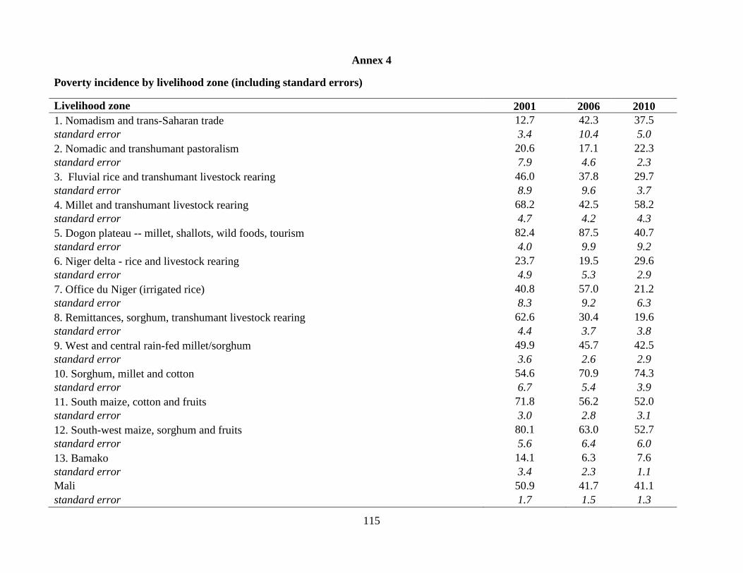
115
Annex 4
Poverty incidence by livelihood zone (including standard errors)
Livelihood zone 2001 2006 2010
1. Nomadism and trans-Saharan trade 12.7 42.3 37.5
standard error 3.4 10.4 5.0
2. Nomadic and transhumant pastoralism 20.6 17.1 22.3
standard error 7.9 4.6 2.3
3. Fluvial rice and transhumant livestock rearing 46.0 37.8 29.7
standard error 8.9 9.6 3.7
4. Millet and transhumant livestock rearing 68.2 42.5 58.2
standard error 4.7 4.2 4.3
5. Dogon plateau -- millet, shallots, wild foods, tourism 82.4 87.5 40.7
standard error 4.0 9.9 9.2
6. Niger delta - rice and livestock rearing 23.7 19.5 29.6
standard error 4.9 5.3 2.9
7. Office du Niger (irrigated rice) 40.8 57.0 21.2
standard error 8.3 9.2 6.3
8. Remittances, sorghum, transhumant livestock rearing 62.6 30.4 19.6
standard error 4.4 3.7 3.8
9. West and central rain-fed millet/sorghum 49.9 45.7 42.5
standard error 3.6 2.6 2.9
10. Sorghum, millet and cotton 54.6 70.9 74.3
standard error 6.7 5.4 3.9
11. South maize, cotton and fruits 71.8 56.2 52.0
standard error 3.0 2.8 3.1
12. South-west maize, sorghum and fruits 80.1 63.0 52.7
standard error 5.6 6.4 6.0
13. Bamako 14.1 6.3 7.6
standard error 3.4 2.3 1.1
Mali 50.9 41.7 41.1
standard error 1.7 1.5 1.3

116