Geological Modeling: Climate-hydrological modeling of

sediment supply

Dr. Irina Overeem Community Surface Dynamics Modeling System

University of Colorado at Boulder

September 2008

2

Course outline 1 •  Lectures by Irina Overeem:

•  Introduction and overview •  Deterministic and geometric models •  Sedimentary process models I •  Sedimentary process models II •  Uncertainty in modeling

•  This Lecture •  Predicting the amount of sediment supplied to a basin •  Quantifying sediment supply processes •  Quantifying input parameters •  Predicting the variability of sediment supply

•  Classroom discussion on paleo-basins

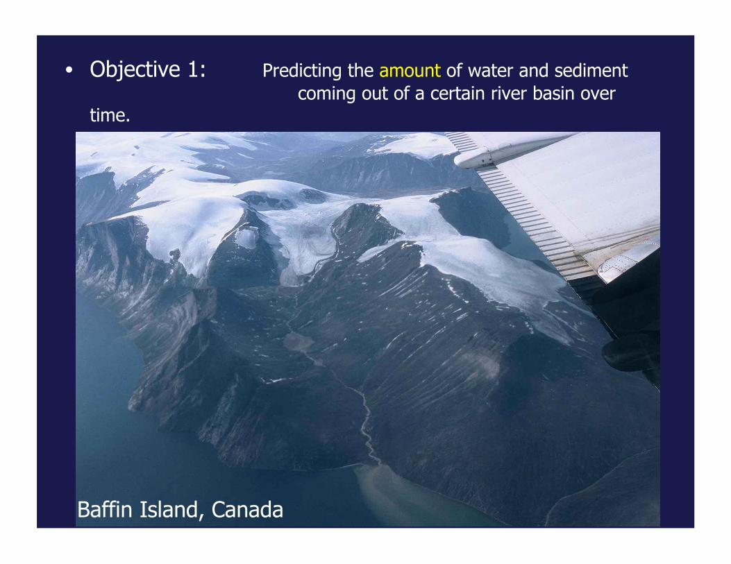
•  Objective 1: Predicting the amount of water and sediment coming out of a certain river basin over

time.

Baffin Island, Canada

4

Classroom Discussion: Constructing the web of sediment supply

•  What are the controls on water supply? •  What are the controls on sediment supply?

•  LIST>>>>>

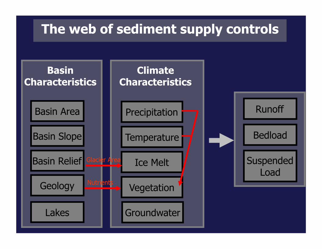
The web of sediment supply controls

Basin Area

Basin Slope

Basin Relief

Geology

Basin Characteristics

Lakes

Precipitation

Temperature

Ice Melt

Vegetation

Climate Characteristics

Groundwater

Runoff

Bedload

Suspended Load

Glacier Area

Nutrients

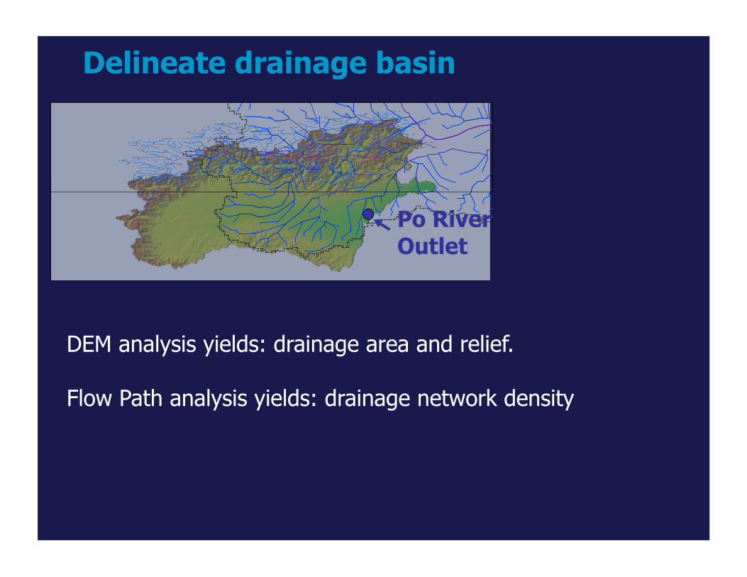
Delineate drainage basin

Po River Outlet

DEM analysis yields: drainage area and relief.

Flow Path analysis yields: drainage network density

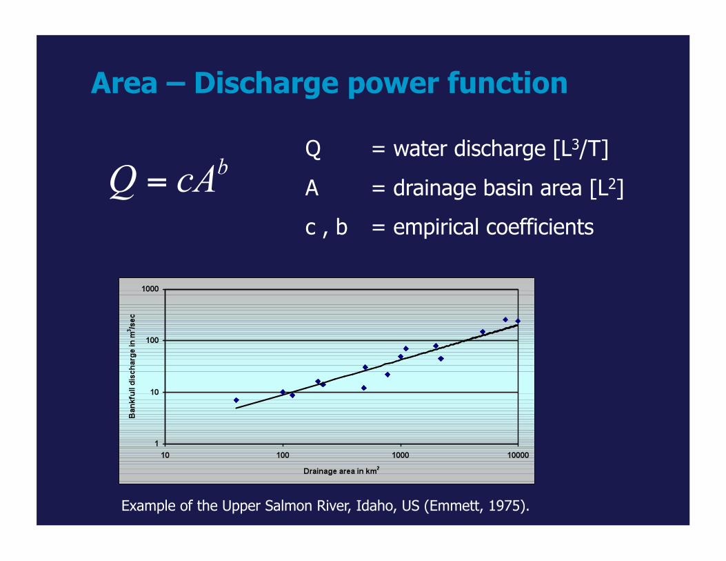
Area – Discharge power function

Q = water discharge [L3/T]

A = drainage basin area [L2]

c , b = empirical coefficients

Example of the Upper Salmon River, Idaho, US (Emmett, 1975).

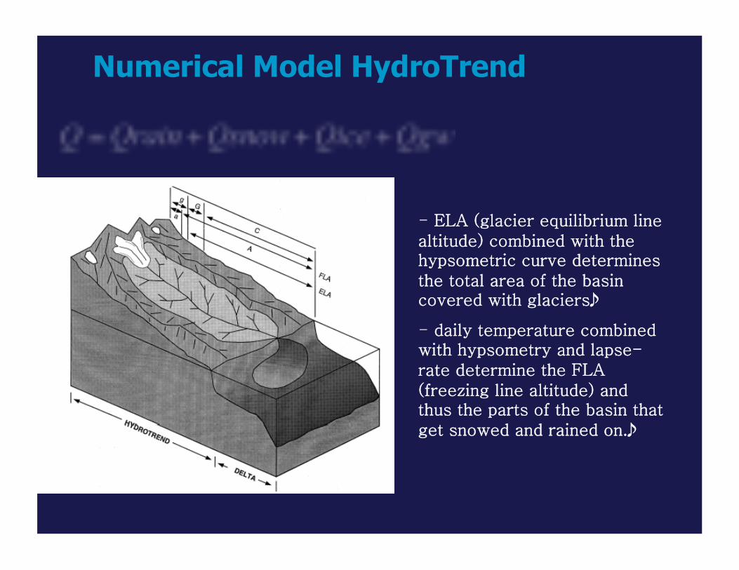
Numerical Model HydroTrend

-  ELA (glacier equilibrium line altitude) combined with the hypsometric curve determines the total area of the basin covered with glaciers

-  daily temperature combined with hypsometry and lapse-rate determine the FLA (freezing line altitude) and thus the parts of the basin that get snowed and rained on.

9

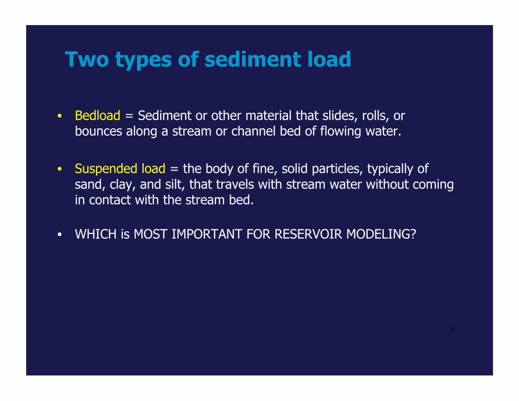
Two types of sediment load

•  Bedload = Sediment or other material that slides, rolls, or bounces along a stream or channel bed of flowing water.

•  Suspended load = the body of fine, solid particles, typically of sand, clay, and silt, that travels with stream water without coming in contact with the stream bed.

•  WHICH is MOST IMPORTANT FOR RESERVOIR MODELING?

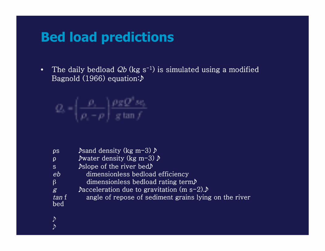
•  The daily bedload Qb (kg s-1) is simulated using a modified Bagnold (1966) equation:

ρs sand density (kg m-3) ρ water density (kg m-3) s slope of the river bed eb dimensionless bedload efficiency β  dimensionless bedload rating term g acceleration due to gravitation (m s-2). tan f angle of repose of sediment grains lying on the river bed

Bed load predictions

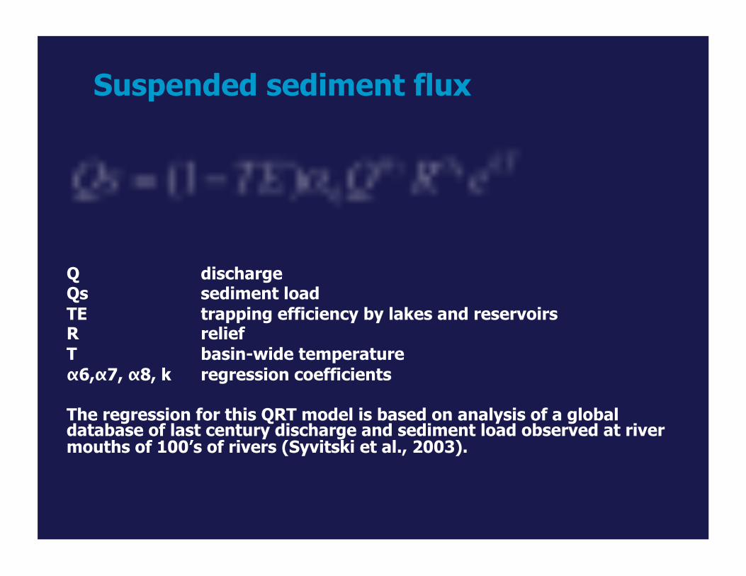
Q discharge Qs sediment load TE trapping efficiency by lakes and reservoirs R relief T basin-wide temperature α6,α7, α8, k regression coefficients

The regression for this QRT model is based on analysis of a global database of last century discharge and sediment load observed at river mouths of 100’s of rivers (Syvitski et al., 2003).

Suspended sediment flux

August 5, 2009 12

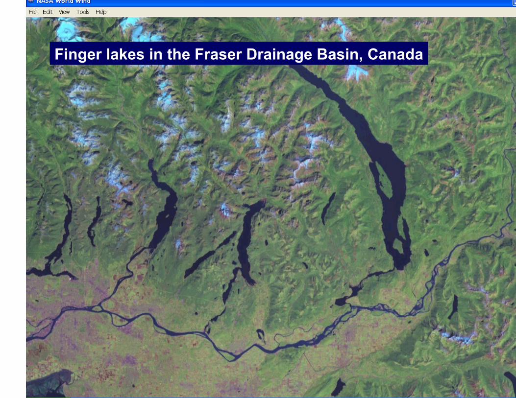
Finger lakes in the Fraser Drainage Basin, Canada

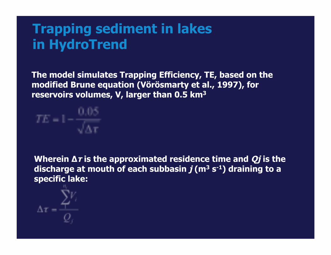
The model simulates Trapping Efficiency, TE, based on the modified Brune equation (Vörösmarty et al., 1997), for reservoirs volumes, V, larger than 0.5 km3

Trapping sediment in lakes in HydroTrend

Wherein ∆τ is the approximated residence time and Qj is the discharge at mouth of each subbasin j (m3 s-1) draining to a specific lake:

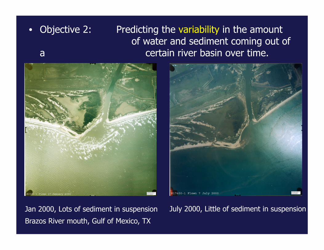
•  Objective 2: Predicting the variability in the amount of water and sediment coming out of

a certain river basin over time.

Jan 2000, Lots of sediment in suspension July 2000, Little of sediment in suspension

Brazos River mouth, Gulf of Mexico, TX

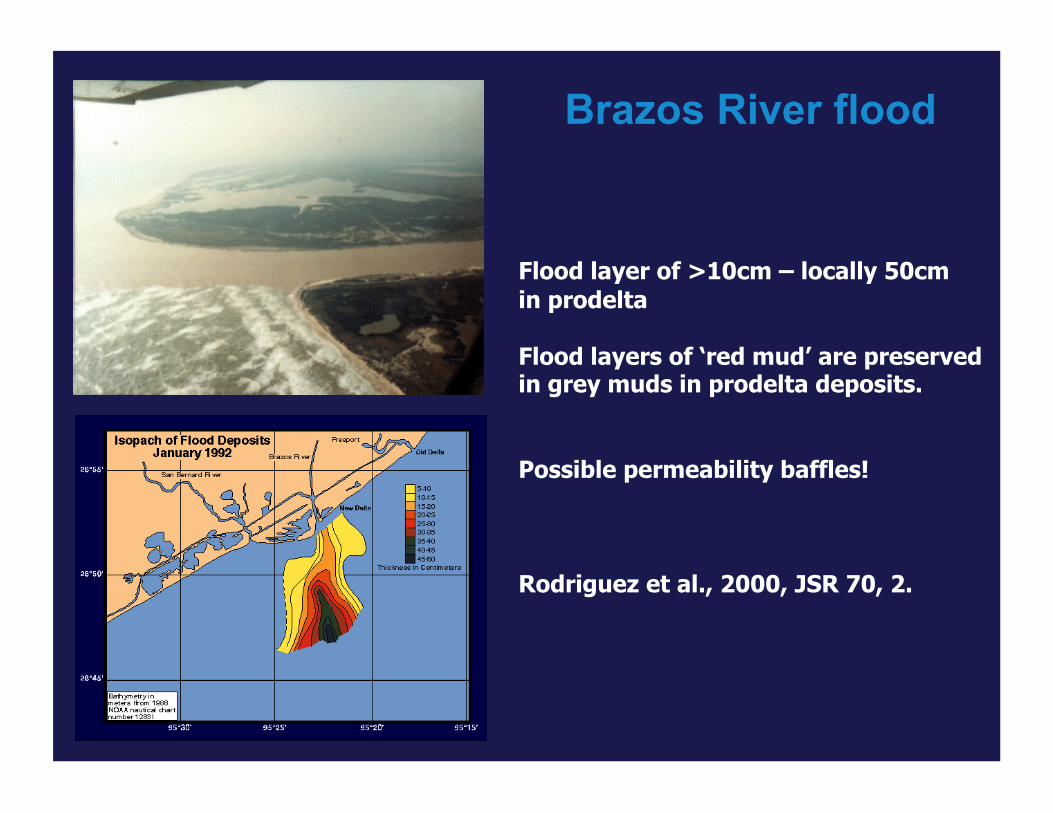
Brazos River flood

Flood layer of >10cm – locally 50cm in prodelta

Flood layers of ‘red mud’ are preserved in grey muds in prodelta deposits.

Possible permeability baffles!

Rodriguez et al., 2000, JSR 70, 2.

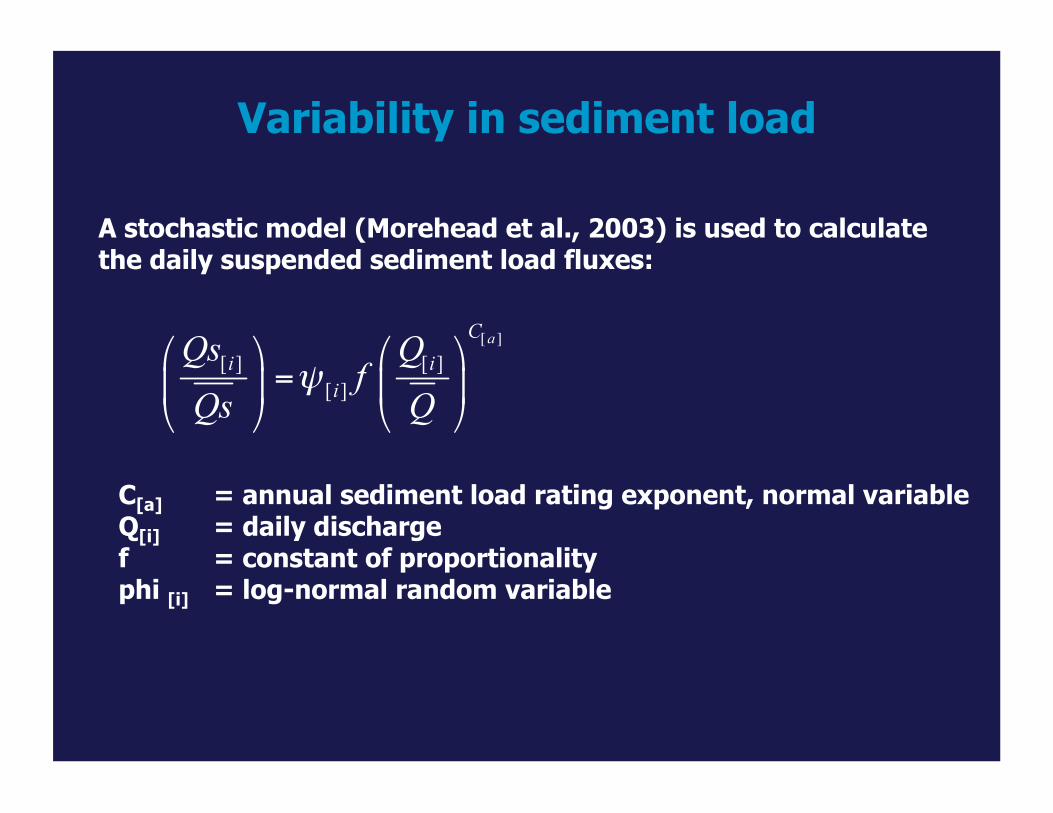
Variability in sediment load

A stochastic model (Morehead et al., 2003) is used to calculate the daily suspended sediment load fluxes:

C[a] = annual sediment load rating exponent, normal variable Q[i] = daily discharge f = constant of proportionality phi [i] = log-normal random variable

17

HydroTrend Model Example

•  Po River, Northern Italy •  100 years validation experiment •  21,000 years simulation

•  Intended as input to a number of stratigraphic models to predict the stratigraphy of the Adriatic basin.

•  Kettner, A.J., and Syvitski, J.P.M., In Press. Predicting discharge and sediment flux of the Po River, Italy since the Last Glacial Maximum, in de Boer, P.L., et al., eds., Analogue and numerical forward modelling of sedimentary systems; from understanding to prediction, International Association of Sedimentologists, special publication, 40.

August 5, 2009 18

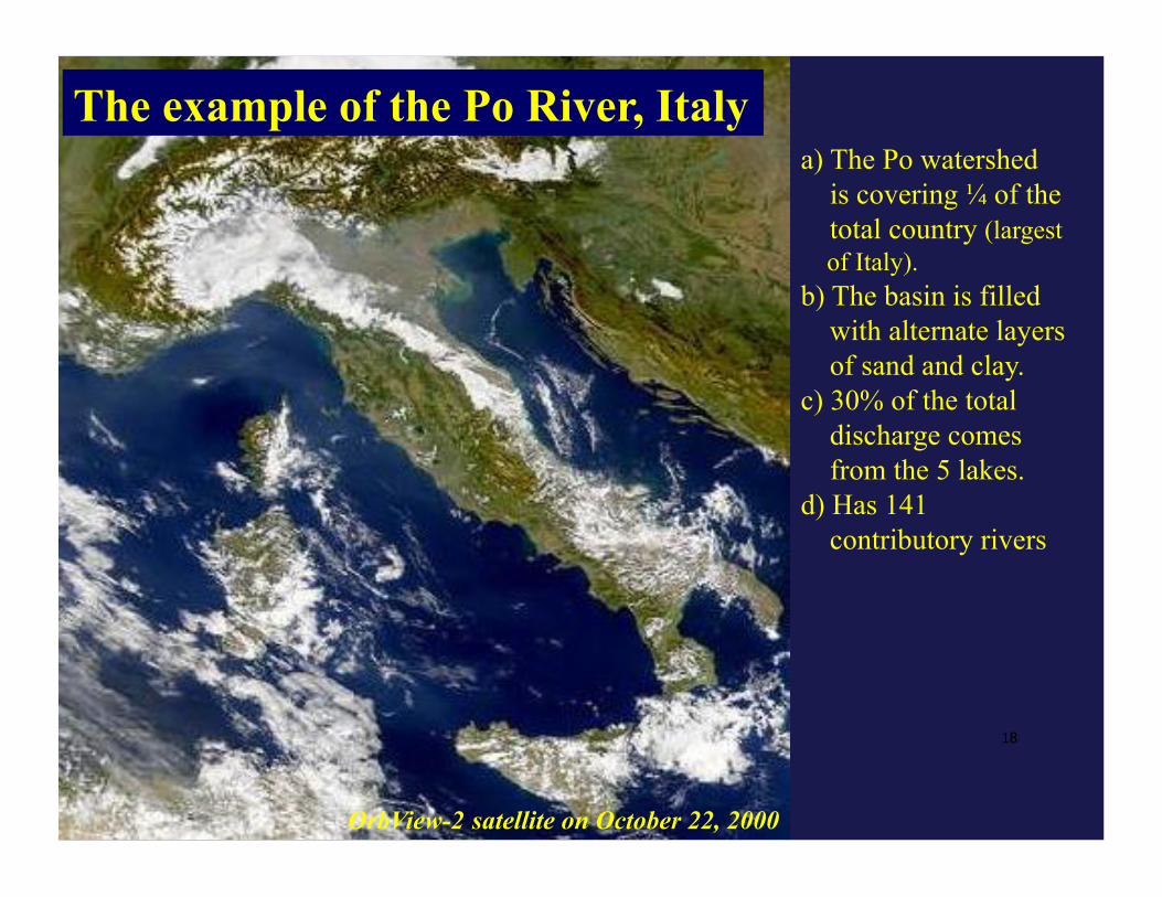
OrbView-2 satellite on October 22, 2000

a) The Po watershed is covering ¼ of the total country (largest of Italy). b) The basin is filled with alternate layers of sand and clay. c) 30% of the total discharge comes from the 5 lakes. d) Has 141 contributory rivers

The example of the Po River, Italy

August 5, 2009 19

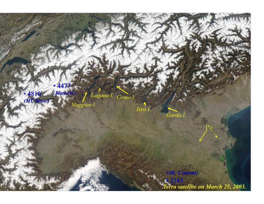
Terra satellite on March 25, 2003.

Garda l.

Como l.

Iseo l. Maggiore l.

Lugano l.

August 5, 2009 20

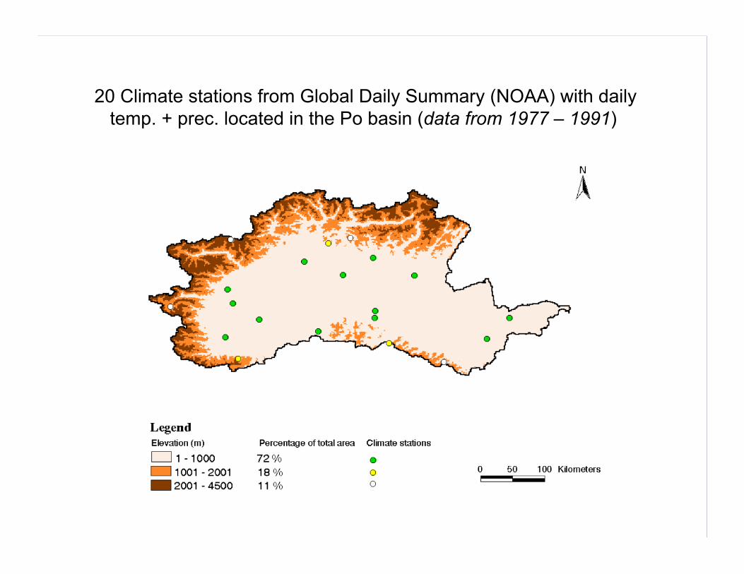
20 Climate stations from Global Daily Summary (NOAA) with daily temp. + prec. located in the Po basin (data from 1977 – 1991)

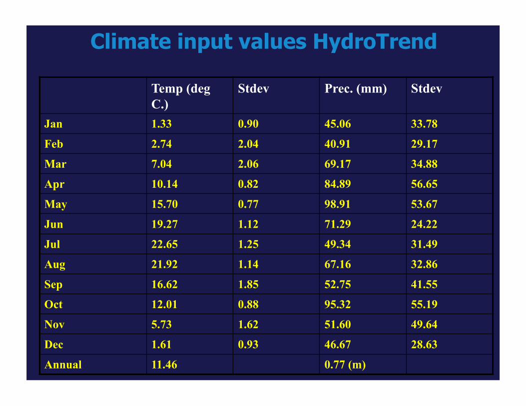
Temp (deg C.)

Stdev Prec. (mm) Stdev

Jan 1.33 0.90 45.06 33.78

Feb 2.74 2.04 40.91 29.17

Mar 7.04 2.06 69.17 34.88

Apr 10.14 0.82 84.89 56.65

May 15.70 0.77 98.91 53.67

Jun 19.27 1.12 71.29 24.22

Jul 22.65 1.25 49.34 31.49

Aug 21.92 1.14 67.16 32.86

Sep 16.62 1.85 52.75 41.55

Oct 12.01 0.88 95.32 55.19

Nov 5.73 1.62 51.60 49.64

Dec 1.61 0.93 46.67 28.63

Annual 11.46 0.77 (m)

Climate input values HydroTrend

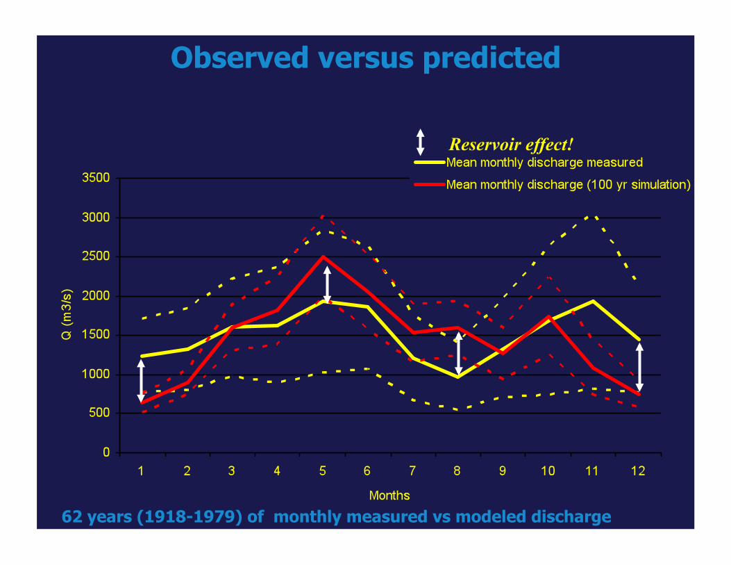
Observed versus predicted

Reservoir effect!

62 years (1918-1979) of monthly measured vs modeled discharge

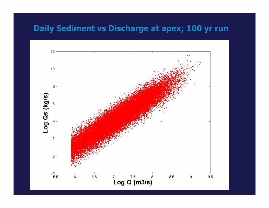
Daily Sediment vs Discharge at apex; 100 yr run

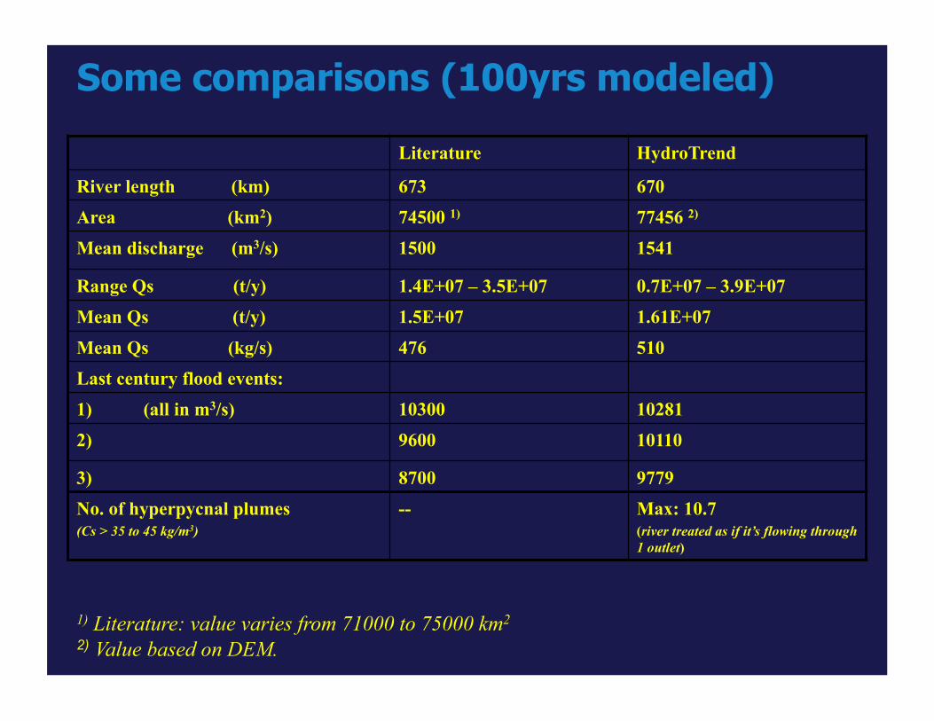
Some comparisons (100yrs modeled)

Literature HydroTrend

River length (km) 673 670 Area (km2) 74500 1) 77456 2)

Mean discharge (m3/s) 1500 1541

Range Qs (t/y) 1.4E+07 – 3.5E+07 0.7E+07 – 3.9E+07 Mean Qs (t/y) 1.5E+07 1.61E+07 Mean Qs (kg/s) 476 510 Last century flood events: 1) (all in m3/s) 10300 10281 2) 9600 10110

3) 8700 9779 No. of hyperpycnal plumes (Cs > 35 to 45 kg/m3)

-- Max: 10.7 (river treated as if it’s flowing through 1 outlet)

1) Literature: value varies from 71000 to 75000 km2

2) Value based on DEM.

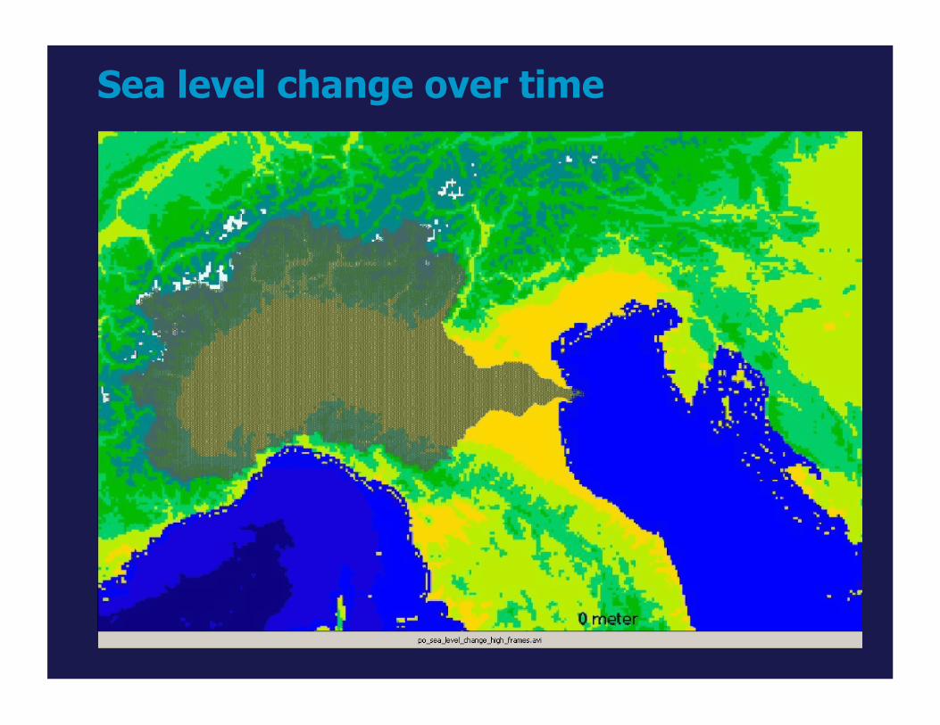
Sea level change over time

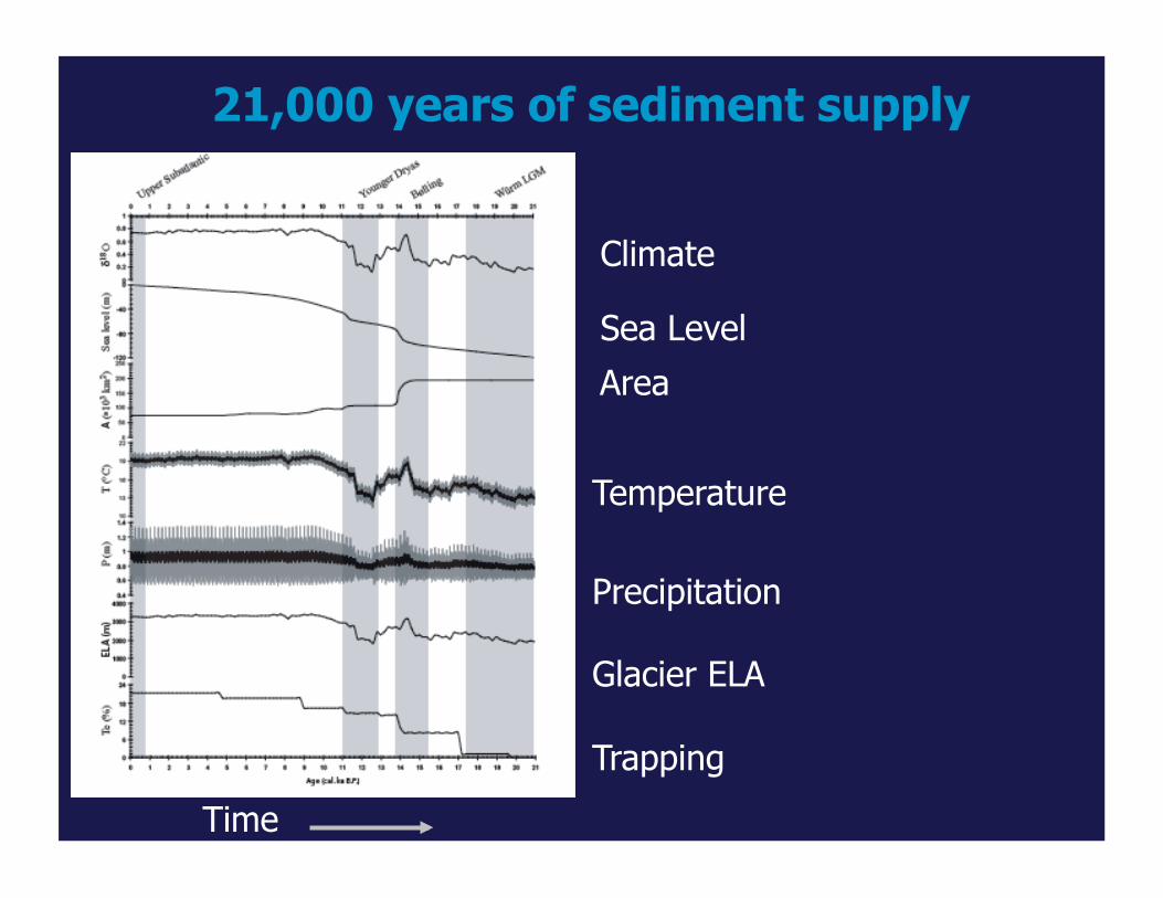
21,000 years of sediment supply

Trapping

Glacier ELA

Precipitation

Time

Temperature

Area

Sea Level

Climate

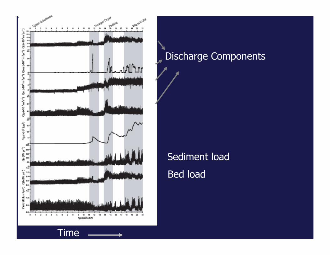
Time

Discharge Components

Sediment load

Bed load

28

References

•  Syvitski, J.P.M., Morehead, M.D., and Nicholson, M, 1998. HydroTrend: A climate-driven hydrologic-transport model for predicting discharge and sediment load to lakes or oceans. Computers and Geoscience 24(1): 51-68.

•  Kettner, A.J., and Syvitski, J.P.M., in press. HydroTrend version 3.0: a Climate-Driven Hydrological Transport Model that Simulates Discharge and Sediment Load leaving a River System. Computers & Geosciences, Special Issue.

29

Classroom discussion

•  Shortcoming of DEM’s for paleo drainage basins? •  What is an alternative strategy?

•  Sources of information for paleo temperature? •  Sources of information for paleo precipitation?

•  How do you quantify variability in proxy data?

•  How can we use ART-equation for paleo river?