GEOMETRIC

ABELIAN CLASS FIELD THEORY

By

Peter Toth

SUBMITTED IN PARTIAL FULFILLMENT OF THE

REQUIREMENTS FOR THE DEGREE OF

MASTER OF SCIENCE

AT

UNIVERSITEIT UTRECHT

MAY 2011

c© Copyright by Peter Toth, 2011

UNIVERSITEIT UTRECHT

DEPARTMENT OF

MATHEMATICS

The undersigned hereby certify that they have read and

recommend to the Faculty of Science for acceptance a thesis entitled

“Geometric Abelian Class Field Theory” by Peter Toth in partial

fulfillment of the requirements for the degree of Master of Science.

Dated: May 2011

Supervisor:Dr. Jochen Heinloth

Formal Supervisor at UUProf. Gunther L.M. Cornelissen

External Examiner:Prof. Frits Beukers

Examing Committee:Prof. Gunther L.M. Cornelissen

Prof. Frits Beukers

ii

To Anett and Belian.

iii

Table of Contents

Table of Contents iv

Abstract vi

Acknowledgements vii

Introduction 2

1 Unramified Geometric Abelian Class Field Theory 5

1.1 The Main Theorem: Artin’s Reciprocity Law . . . . . . . . . . . . . . 6

1.2 Symmetric Powers of a Curve . . . . . . . . . . . . . . . . . . . . . . 14

1.3 The Picard Scheme of a Curve . . . . . . . . . . . . . . . . . . . . . . 20

1.4 The Etale Fundamental Group . . . . . . . . . . . . . . . . . . . . . . 24

1.5 l-adic Local Systems and Representations . . . . . . . . . . . . . . . . 31

1.6 The Faisceaux-Fonctions Correspondence . . . . . . . . . . . . . . . . 38

2 The Proof of the Main Theorem of the Unramified Theory 43

2.1 Preliminary Constructions . . . . . . . . . . . . . . . . . . . . . . . . 43

2.2 Deligne’s Geometric Proof . . . . . . . . . . . . . . . . . . . . . . . . 50

3 Tamely Ramified Geometric Abelian Class Field Theory 65

3.1 The Main Theorem . . . . . . . . . . . . . . . . . . . . . . . . . . . . 66

3.2 The Symmetric Power U (d) and the relative Picard Scheme PicC,S . . 74

3.3 The Tame Fundamental Group . . . . . . . . . . . . . . . . . . . . . 77

4 The Proof of the Main Theorem of the Tamely Ramified Theory 83

4.1 Preliminary Constructions . . . . . . . . . . . . . . . . . . . . . . . . 83

4.2 A Geometric Proof . . . . . . . . . . . . . . . . . . . . . . . . . . . . 90

iv

Bibliography 105

v

Abstract

The purpose of this thesis has been twofold. First to give a detailed treatment of

unramified geometric abelian class field theory concentrating on Deligne’s geometric

proof in order to remedy the unfortunate situation that the literature on this topic is

very deficient, partial and sketchy written1. In the second place to give also a detailed

treatment of ramified geometric abelian class field theory and more importantly to

find a new geometric proof for the ramified theory by trying to adapt or to lean on

Deligne’s geometric argument in the unramified case.

What was achieved is the following: we begin with discussing and building up the

unramified theory in details, which describes a remarkable connection between the

Picard group and the abelianized etale fundamental group of a smooth, projective,

geometrically irreducible curve over a finite field. We give the necessary background

culminating in the fully presented geometric proof of Deligne. Then we turn to

a detailed discussion of the tamely ramified theory, which transforms the classical

situation to the open complement of a finite set of points of the curve, establishing

a connection between a modified Picard group and the tame fundamental group of

the curve with respect to this finite subset of points. In the end we finally present a

geometric proof for the tamely ramified theory.

1Probably due to the fact that people working on this field are mostly concentrating on the higherdimensional theory, that is on the geometric Langlands program, instead of writing down relativelyclassical works in a fairly didactic way.

vi

Acknowledgements

First and foremost I am very grateful to my supervisor Dr. Jochen Heinloth, who

unintendedly was able to give me THE master thesis theme I have been looking for. He

patiently introduced me into this wonderful topic and taught me a lot of mathematics

especially by answering all my painful questions on our regular meetings. His help

and support was really invaluable and I hope we will continue to work in some sense,

in some time...

I am very grateful to my formal supervisor Prof. Gunther L.M. Cornelissen, who

hosted my thesis at Utrecht University, read the final version and has been one of the

member of the Examing Committee. Also I am thankful to Prof. Frits Beukers to be

an external reader and the other member of the Examing Committee.

I am very grateful to Prof. Gavril Farkas who helped me a lot to be able to come

to the Netherlands and to participate on the MRI Master Class 2010/2011 Moduli

Spaces, which was the main reason for that I finished my undergraduate studies in

Utrecht instead of Berlin. I wish to thank the organizers, lecturers and participants

of the Master Class for the great time I had with them.

I thank a lot my soul-keeping brothers, Dimiter and Gabor, also to Kriszta and

Balazs and to my family in Hungary.

At last but not least I am very grateful, thankful and everythingful to my wife

Anett and my son, Belian for constantly supporting, encouraging and loving me...

Utrecht, The Netherlands Peter Toth

May 15, 2011

vii

...d¨lon gr ±c ÍmeØc màn taÜta (tÐ pote boÔlesje shmaÐnein åpìtan >än

fjèggesje) plai gign¸skete, meØc dà prä toÜ màn ¶ìmeja, nÜn d' por kamen...

...for manifestly you have long been aware of what you mean when you use

the expression ’being’. We, however, who used to think we understood it,

have now become perplexed...

Plato, Sophist 244a

Introduction

Abelian class field theory aims to provide a description of the abelian extensions of

a global field K in terms of arithmetic data attached to it. A natural way to encode

this information is to consider all algebraic extensions of K at once resulting the

big Galois group Gal(K/K) and take its abelianization Gal(Kab/K) describing the

abelian extensions. The main goal is then to capture this Galois world relying on the

arithmetic of the field K.

Mysteriously the suitable arithmetic data associated to the field K is its idele

group IK which is a topological group defined by the restricted product

IK :=∏′

vK×v

using the completions Kv at all primes (places) of the field K. On the Galois side

one can associate to each prime v of K the Frobenius element Frobv ∈ Gal(Kab/K)

which enables us to define Artin’s Reciprocity Map

ΦK : IK −→ Gal(Kab/K)

given by

ΦK : (. . . , av, . . . ) 7→∏

v Frobordv(av)v .

2

3

For precise definitions and proofs of the statements what follows the reader is referred

to the classical references, such as V.5. in [Mil08b] and Chapters VII., VIII. in [AT90].

Different base fields need different treatments and provide different end results.

For number fields the high-light of the classical theory is Artin’s Reciprocity Law,

which states that the Reciprocity Map is surjective and factors through the idele

class group CK := K×\IK of K giving an isomorphism

ΦK : CK/O∼=−→ Gal(Kab/K)

where O is the connected component of 1 ∈ CK .

For function fields the Reciprocity Map is no longer surjective but factors also

through the the idele class group and results an injective map with dense image

ΦK : K×\IK/∏

vO×v → Gal(Kab/K).

In this thesis we will concentrate on the function field case, i.e. geometric abelian

class field theory, starting with the unramified theory where we take the function field

K = k(C) of a smooth, projective, geometrically irreducible curve C defined over a

finite base field k = Fq and consider all abelian unramified extensions Gal(Kun/K)ab.

We will proceed with the theory in a geometric manner interpreting the Reciprocity

Map in purely geometric terms, namely the adelic double quotient on the left hand

side can be identified with the Picard group PicC(k) of C and on the Galois side we

have the ablianized etale fundamental group πab1 (C). Then relying on brilliant ideas

of Deligne in order to prove Artin’s Reciprocity Law we will begin a long geometric

journey going on a by-pass road through l-adic representations, l-adic local systems

and Grothendieck’s faisceaux-fonctions correspondence leading finally to a geometric

proof of the unramified theory.

4

Then we turn our attention to the tamely ramified theory considering a finite set

of points S ⊂ C and its open complement U := C \ S and we transplant the results

of the unramified theory by establishing a Reciprocity Map

ΦK,S : PicC,S(k) −→ πt,ab1 (U)

between the k-rational points of a modified Picard group and the abelianized tame

etale fundamental group of C with respect to S. In this case we will be able to adapt

Deligne’s geometric argument leading to a geometric proof for the tamely ramified

theory.

Geometric class field theory is now embedded as the one dimensional case in

big theories, such as the geometric Langlands Program or higher dimensional class

field theory. There are many references for the subject, but as far as I know none

of them endeavors completeness and/or does particularly not dwell into the details

concerning Deligne’s geometric proof in this one dimensional case. A good overview is

given in [Fre05] or in [Gai04]. Deligne’s argument is contained in [Lau90], [Hei07] and

[Hei04]. We give later specific references for all other geometric instruments needed

for fulfilling Deligne’s idea. In the higher dimensional class field theory direction we

refer to [Sch05], which gives a detailed overview and [SS99] which deals with our

subject in a different way. Based upon these articles, the concerned reader will find

other useful references in these directions. I want to mention also [Sza09a] and last

but not least the classical book of Serre [Ser88], which gives a self-contained geometric

approach discussing also the ramified case, but with slightly different end results and

particularly with different techniques.

Chapter 1

Unramified Geometric AbelianClass Field Theory

In this chapter we will present unramified geometric abelian class field theory which

establishes a remarkable connection between the Picard group and the abelianized

etale fundamental group of a smooth projective curve over a finite field.

We begin with stating the main theorem of the unramified theory in different

forms without going into the details and trace out a way how we will prove it.

Then in the subsequent sections we will discuss and develop the background needed

to fully understand and to be able to follow in details the theory. In particular we

will define the basic concepts appearing in both sides of the correspondence, namely

the Picard scheme and the etale fundamental group of a smooth, projective curve

and we will also perform the necessary constructions leading to a proof of the main

theorem, which finally will be provided in the next chapter.

5

6

1.1 The Main Theorem: Artin’s Reciprocity Law

Let C be a smooth, projective, geometrically irreducible curve over a finite field

k = Fq. Let K = k(C) be its function field and for every closed point p ∈ |C| let

Op be the completion of the local ring at the point p and Kp its quotient field. Let

AK :=∏′

p∈|C|Kp be the ring of adeles and IK the idele group of C. Recall that every

p ∈ |C| defines an (additive) discrete valuation ordp of the field K and for an idele

(. . . , ap, . . . )p∈|C| it holds that for all but finitely many p ∈ |C| ordp(ap) = 0. The

main theorem of unramified geometric abelian class field theory is the following:

Theorem 1.1.1 (Artin’s Reciprocity Law, adelic form). The Artin Reciprocity Map

ΦK : IK/∏

p∈|C| O×p πab1 (C)

[(. . . , ap, . . . )p∈|C|]∏

p∈|C| Frobordp(ap)p

ΦK

factors through the quotient

ΦK : K×\IK/∏

p∈|C| O×p πab1 (C)ΦK

and fits into the commutative diagram

Ker(deg) K×\IK/∏

p∈|C| O×p Z

Ker(ϕ) πab1 (C) Z

deg

ϕ

ΦK can

such that there is an induced isomorphism on the kernels

Ker(deg)∼=−→ Ker(ϕ)

7

where ϕ : πab1 (C) −→ Z is the map between the abelianized etale fundamental groups

induced by the structure morphism C −→ Spec(k) (section 1.4).

We can characterize the adelic double quotient in terms of geometric data associ-

ated to the curve C in the following way

Proposition 1.1.2. There is an isomorphism

K×\IK/∏

p∈|C| O×p ∼= PicC(k)

between the adelic double coset space and isomorphism classes of invertible sheaves

on C.

Proof. This is a special case of the more general statement (cf. 2.1 in [Gai04]), which

gives an adelic description of isomorphism classes of vector bundles on C.1

Given an invertible sheaf F on C, we choose a trivialization at the generic point

ξ of C

fξ : F ⊗OC K∼=−→ K

as the local ring Oξ is isomorphic to the function field K. We choose also a trivial-

ization for every closed point p ∈ |C|

fp : F ⊗OC Op∼=−→ Op

as Fp is a free Op-module of rank 1. The natural morphism Op −→ K induces the

diagram

1There is a one-to-one correspondence between isomorphism classes of vector bundles of rank non C and the double coset space GLn(K)\GLn(AK)/

∏p∈|C|GLn(Op).

8

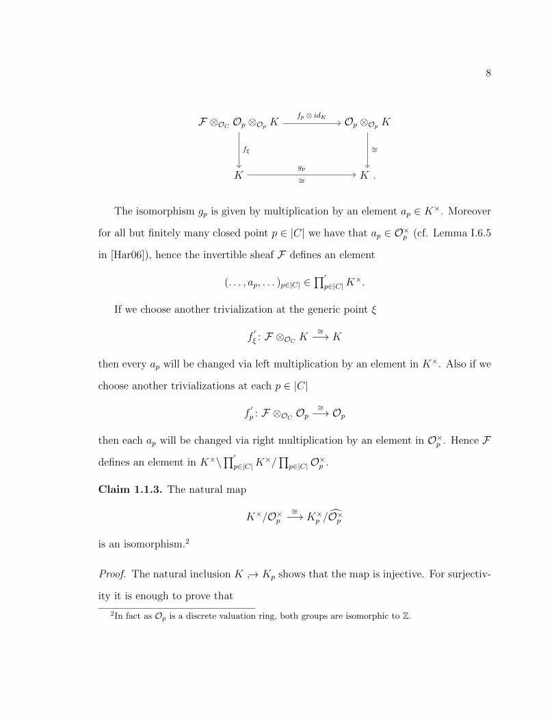
F ⊗OC Op ⊗Op K Op ⊗Op K

K K .

fp ⊗ idK

fξ

∼=

gp

∼=

The isomorphism gp is given by multiplication by an element ap ∈ K×. Moreover

for all but finitely many closed point p ∈ |C| we have that ap ∈ O×p (cf. Lemma I.6.5

in [Har06]), hence the invertible sheaf F defines an element

(. . . , ap, . . . )p∈|C| ∈∏′

p∈|C|K×.

If we choose another trivialization at the generic point ξ

f′

ξ : F ⊗OC K∼=−→ K

then every ap will be changed via left multiplication by an element in K×. Also if we

choose another trivializations at each p ∈ |C|

f′p : F ⊗OC Op

∼=−→ Op

then each ap will be changed via right multiplication by an element in O×p . Hence F

defines an element in K×\∏′

p∈|C|K×/

∏p∈|C|O×p .

Claim 1.1.3. The natural map

K×/O×p∼=−→ K×p /O×p

is an isomorphism.2

Proof. The natural inclusion K → Kp shows that the map is injective. For surjectiv-

ity it is enough to prove that

2In fact as Op is a discrete valuation ring, both groups are isomorphic to Z.

9

K×p = K×O×p .

Let a ∈ K×p be given. By Theorem II.4.4 in [Neu07] we can write a uniquely as

a = uπm(a0 + a1π + a2π2 + . . . )

where u ∈ O×p , π ∈ Op is a primelement ordp(π) = 1, m ∈ Z, ai ∈ R ⊂ Op, where R

is a representative system for the residue field Op/mp, a0 6= 0, hence

(a0 + a1π + a2π2 + . . . ) ∈ O×p .

By Theorem II.3.8 in [Neu07] we have that uπm ∈ K× completing the proof of the

claim.

Now we use this isomorphism to get an element in K×\IK/∏

p∈|C| O×p defined by F ,

which depends only on the isomorphism class of F by construction.

On the other hand given an element a = (. . . , ap, . . . ) ∈ IK we define a sheaf Fa

on C by

Fa(U) := x ∈ K| a−1p x ∈ Op ∀ p ∈ U.

It follows from this local description that Fa defines a sheaf on C. Moreover changing

the coset representative a from the right by an element in∏

p∈|C| O×p does not change

anything in Fa and changing from the left by an element b ∈ K× gives an isomorphism

of sheaves Fab×−→ Fba, so the only thing to prove is that Fa is locally free of rank

1. If ap ∈ O×p for all p ∈ U then Fa(U) = OC(U) by construction, hence it is free

on U . Otherwise using the above claim 1.1.3 we take an element t ∈ K× such that

tap ∈ O×p . Now define U := p ∈ |C| : t ∈ O×p and use the isomorphism Fat×−→ Fta

which gives that Fa is locally free of rank 1 on U .

These two constructions are inverses to each other which completes the proof.

10

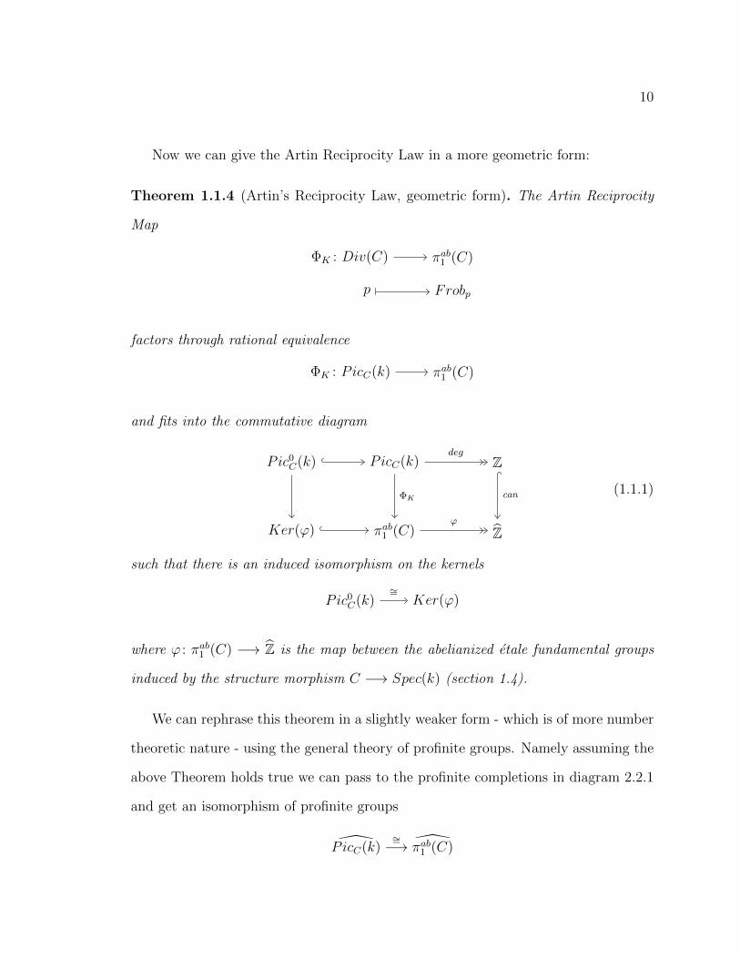
Now we can give the Artin Reciprocity Law in a more geometric form:

Theorem 1.1.4 (Artin’s Reciprocity Law, geometric form). The Artin Reciprocity

Map

ΦK : Div(C) πab1 (C)

p Frobp

factors through rational equivalence

ΦK : PicC(k) πab1 (C)

and fits into the commutative diagram

Pic0C(k) PicC(k) Z

Ker(ϕ) πab1 (C) Z

deg

ϕ

ΦK can (1.1.1)

such that there is an induced isomorphism on the kernels

Pic0C(k) Ker(ϕ)

∼=

where ϕ : πab1 (C) −→ Z is the map between the abelianized etale fundamental groups

induced by the structure morphism C −→ Spec(k) (section 1.4).

We can rephrase this theorem in a slightly weaker form - which is of more number

theoretic nature - using the general theory of profinite groups. Namely assuming the

above Theorem holds true we can pass to the profinite completions in diagram 2.2.1

and get an isomorphism of profinite groups

PicC(k)∼=−→ πab1 (C)

11

by Corollary 10.3 in [AM69] (as the isomorphism Pic0C(k)

∼=−→ Ker(ϕ) induces an

isomorphism between the completions andZ = Z, hence there is an isomorphism

between the completions in the middle).

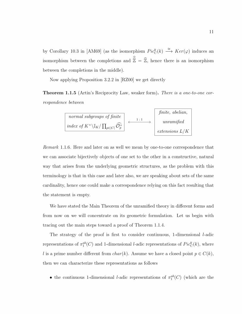
Now applying Proposition 3.2.2 in [RZ00] we get directly

Theorem 1.1.5 (Artin’s Reciprocity Law, weaker form). There is a one-to-one cor-

respondence between

normal subgroups of finite

index of K×\IK/∏

p∈|C| O×p

finite, abelian,

unramified

extensions L/K

1 : 1

Remark 1.1.6. Here and later on as well we mean by one-to-one correspondence that

we can associate bijectively objects of one set to the other in a constructive, natural

way that arises from the underlying geometric structures, as the problem with this

terminology is that in this case and later also, we are speaking about sets of the same

cardinality, hence one could make a correspondence relying on this fact resulting that

the statement is empty.

We have stated the Main Theorem of the unramified theory in different forms and

from now on we will concentrate on its geometric formulation. Let us begin with

tracing out the main steps toward a proof of Theorem 1.1.4.

The strategy of the proof is first to consider continuous, 1-dimensional l-adic

representations of πab1 (C) and 1-dimensional l-adic representations of Pic0C(k), where

l is a prime number different from char(k). Assume we have a closed point p ∈ C(k),

then we can characterize these representations as follows

• the continuous 1-dimensional l-adic representations of πab1 (C) (which are the

12

same as the continuous 1-dimensional l-adic representations of the algebraic fun-

damental group π1(C, s)) are in one-to-one correspondence with 1-dimensional

l-adic local systems L on C together with a rigidification, i.e. a fixed isomor-

phism ϕ : Ls ∼= Ql, where s : Spec(Ω) −→ C is a geometric point (cf. section

1.5);

• 1-dimensional l-adic representations of Pic0C(k) together with a Frobenius action

Frobp : Z −→ Q×l are in one-to-one correspondence with 1-dimensional l-adic

local systems AL on PicC together with a rigidification, i.e. a fixed isomorphism

ψ : AL|0 ∼= Ql satisfyingm−1Ad+eL∼= AdLAeL, wherem : PicdC×PiceC −→ Picd+e

C

is the group operation on PicC and 0: Spec(k) → Pic0C is the identity section

(the class of the trivial bundle) (cf. section 1.6).

Using these correspondences we will present Deligne’s geometric argument in sec-

tion 2.2, which gives a one-to-one correspondence between rigidified 1-dimensional

l-adic local systems on C and rigidified multiplicative 1-dimensional l-adic local sys-

tems on PicC . Having done this we will get the following diagram:

13

continous 1-dimensional

l-adic representations of

πab1 (C) χ : πab1 (C) → Q×l

1-dimensional l-adic rep-

resentations of Pic0C(k)

χ : Pic0C(k) → Q×l

together with a Frobenius

action Frobp : Z → Q×l

1-dimensional l-adic

local systems L on C

together with a fixed

isomorphism ϕ : Ls ∼= Ql

1-dimensional l-adic

local systems AL on

PicC together with

a fixed isomorphism

ψ : AL|0 ∼= Ql satisfying

m−1Ad+eL = AdL AeL

1 : 1

1 : 1

Deligne

1 : 1

faisceaux-fonctions1 : 1(1.1.2)

Finally in section 2.2 we will use the correspondences appearing in this diagram

to prove Artin’s Reciprocity Law.

14

1.2 Symmetric Powers of a Curve

In this section we will recall the construction of symmetric powers of a curve over a

field k and investigate their relationship to effective divisors on the curve. The main

references will be [Mum70] and [Mil08a].

First we will work in a fairly general setting and then descend to the case of curves.

So let X be a quasi-projective scheme of finite presentation over a field k. For an

integer d ≥ 1 let us consider the d-fold product

Xd := X ×Spec(k) · · · ×Spec(k) X.

There is an action of the symmetric group Sd on Xd by permuting the factors.

Definition 1.2.1. A morphism g : Xd −→ Y of schemes over k is said to be sym-

metric if it is invariant under the Sd action on Xd.

Then the main theorem is the following:

Theorem 1.2.2. Let X be a quasi-projective scheme of finite presentation over a

field k and d ≥ 1 a positive integer. Then there exists a scheme X(d) over k and

a symmetric morphism π : Xd −→ X(d) called the dth symmetric power of the

scheme X/k having the following properties:

1. the underlying topological space is the quotient X(d) := Xd/Sd of Xd by the

action of Sd;

2. for an affine open subset U ⊂ X, U (d) ⊂ X(d) is affine open and it holds that

OX(d)(U (d)) = (OXd(Ud))Sd.

15

The pair (X(d), π) has the following universal property: every symmetric k-morphism

g : Xd −→ Y factors uniquely through π and (X(d), π) is uniquely determined up

to a unique isomorphism by this universal property. Moreover the map π is finite,

surjective and separated.

Proof. See II.7 in [Mum70].

In the case of curves we have additionally the very important property:

Proposition 1.2.3. Let C be a nonsingular curve over a field k and d ≥ 1 a positive

integer. Then the dth symmetric power C(d) is also nonsingular.

Proof. See Proposition 3.2. in [Mil08a] and Proposition 11.24 in [AM69].

Next we turn to the connection between effective divisors and symmetric powers.

First we note the following

Proposition 1.2.4. For a noetherian, integral, locally factorial separated scheme X

the group Div(X) of Weil divisors on X is isomorphic to the group of Cartier divi-

sors H0(X,K∗/O∗X) on X (principal Weil divisors corresponding to principal Cartier

divisors).

Proof. This is Proposition 6.11 in [Har06].

Now we define effective Cartier divisors in a relative situation.

Definition 1.2.5. Let f : X −→ T be a morphism of schemes over k. A relative

effective Cartier divisor on X/T is an effective Cartier divisor D on X, which is flat

over T considered as a subscheme of X.

16

If the base scheme is affine T = Spec(A), then a subscheme D ⊂ X is a relative

effective Cartier divisor, if there exists an open affine covering X =⋃i∈I Spec(Ai)

such that for all i ∈ I

1. D⋂Spec(Ai) = Spec(Ai/(hi)) where hi ∈ Ai is not a zero divisor

2. Ai/(hi) is a flat A-algebra.

We can characterize relative effective Cartier divisors D on X/T in the following

way. Assume D is represented by (Ui, gi)i∈I where X =⋃i∈I Ui is an open covering,

and gi ∈ Γ(Ui,OX) such that for all i, j, gigj∈ Γ(Ui ×X Uj,O∗X). Then the ideal sheaf

I(D) of the relative effective Cartier divisor D is the invertible sheaf defined locally

on Ui by gi, denoted also by O(−D) suggesting that the invertible sheaf O(D) is

defined locally on Ui by 1gi

. So we have the exact sequence of sheaves on X

0 −→ O(−D) −→ OX −→ OD −→ 0

whereOD is the structure sheaf ofD considered as a closed subscheme ofX. Tensoring

by O(D) we get the exact sequence of sheaves X

0 −→ OXsD−→ O(D) −→ O(D)/sDOX −→ 0

where sD is the canonical non-zero global section of O(D) defined by the inclusion

OX → O(D), such that the subscheme defined by sD is flat over T .

Proposition 1.2.6. The map D 7→ (O(D), sD) establishes a one-to-one correspon-

dence between relative effective Cartier divisors D on X/T and isomorphism classes

of pairs (G, s), where G is a locally free OX-module of rank 1 and s ∈ H0(X,G) \ 0

is a non-zero global section such that the subscheme defined by s is flat over T .

17

Proof. See Remark 3.6. in [Mil08a].

Next we state some basic properties of relative effective Cartier divisors.

Proposition 1.2.7. 1. Let D1 and D2 be relative effective Cartier divisors for

X/T . Then also the sum D1 + D2 is a relative effective Cartier divisor for

X/T .

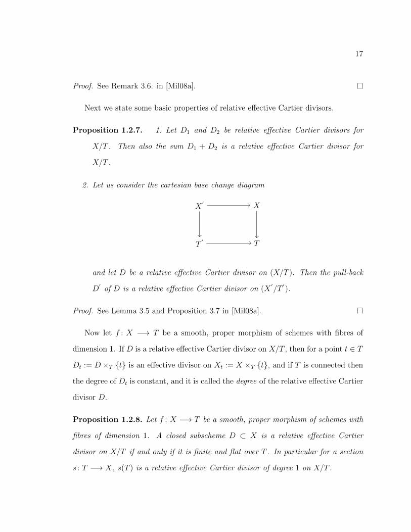
2. Let us consider the cartesian base change diagram

X′

X

T′

T

and let D be a relative effective Cartier divisor on (X/T ). Then the pull-back

D′

of D is a relative effective Cartier divisor on (X′/T′).

Proof. See Lemma 3.5 and Proposition 3.7 in [Mil08a].

Now let f : X −→ T be a smooth, proper morphism of schemes with fibres of

dimension 1. If D is a relative effective Cartier divisor on X/T , then for a point t ∈ T

Dt := D ×T t is an effective divisor on Xt := X ×T t, and if T is connected then

the degree of Dt is constant, and it is called the degree of the relative effective Cartier

divisor D.

Proposition 1.2.8. Let f : X −→ T be a smooth, proper morphism of schemes with

fibres of dimension 1. A closed subscheme D ⊂ X is a relative effective Cartier

divisor on X/T if and only if it is finite and flat over T . In particular for a section

s : T −→ X, s(T ) is a relative effective Cartier divisor of degree 1 on X/T .

18

Proof. Corollary 3.9. in [Mil08a].

Now we restrict ourselves to the case of smooth, projective curves over a field k

and we define the following functor:

Definition 1.2.9. Let C be a smooth, projective curve over a field k, d ≥ 1 a positive

integer and define the functor

DivdC : Sch/k −→ Set

which to a k-scheme T associates the set DivdC(T ) of relative effective Cartier divisors

of degree d on (C ×Spec(k) T )/T .

By the above Proposition 1.2.7 this is well-defined concerning morphisms. For

the proof that this functor is representable by C(d), we construct a canonical rela-

tive effective Cartier divisor on (C ×Spec(k) C(d))/C(d). For that let us consider the

projection

pr : C ×Spec(k) Cd −→ Cd

which has canonical sections for all i = 1, . . . , d

si : Cd −→ C ×Spec(k) Cd

defined by

si((p1, p2, . . . , pd)) := (pi, (p1, p2, . . . , pd)).

Then define the relative effective Cartier divisor D =∑d

i=1Di on C×Spec(k)Cd/Cd,

where Di := si(Cd) is a relative effective Cartier divisor for all i = 1, . . . , d. The

19

divisor D is stable as a subscheme under the action of Sd, and so is Cd, hence it

defines a relative effective Cartier divisor Dcan on C ×Spec(k) C(d)/C(d).

Now we can state the main theorem about the representability of the relative

effective Cartier divisor functor:

Theorem 1.2.10. Let C be a smooth, projective curve over a field k and d ≥ 1 a

positive integer. Then for any relative effective Cartier divisor D on (C×Spec(k) T )/T

there exists a unique morphism α : T −→ C(d) such that

D = (idC × α)−1(Dcan),

that is the functor DivdC is representable by C(d).

Proof. This is Theorem 3.13 in [Mil08a].

20

1.3 The Picard Scheme of a Curve

In this section let C be a smooth, projective curve over a field k. We will define Picard

functors PicdC of various degrees from the category of k-schemes to the category of

abelian groups and investigate under which circumstances are these representable by

a group scheme, denoted also by PicdC over k, such that the k-rational points of this

group scheme should be isomorphic to the group of invertible sheaves of degree d on

C.

First assume for simplicity that C(k) 6= ∅ and let p ∈ C(k) be a k-rational point.

Definition 1.3.1. For an integer d ∈ Z define the Picard functor of degree d of C as

the functor from the category of schemes over k to the category of abelian groups

PicdC : Sch/k −→ Ab

which to a k-scheme T associates the abelian group

PicdC(T ) := G ∈ Pic(C ×Spec(k) T )| deg(Gt) = d ∀t ∈ T/pr−12 (Picd(T ))

i.e. families of invertible sheaves of degree d on C parametrized by T modulo those

coming from T .

We note that for any d ∈ Z and a scheme T over k we have an isomorphism

Pic0C(T )

∼=−→ PicdC(T )

given by

G 7→ G ⊗ pr−11 O(dp).

21

Remark 1.3.2. Hence concerning representability of the Picard functors it is enough

to prove that a Picard functor of some appropriate degree d is representable. Now

the main theorem is the following

Theorem 1.3.3. There exists an abelian variety Jac over k and a natural transfor-

mation of functors α : Pic0C −→ hJac (where hJac is the functor of points of Jac) such

that α(T ) : Pic0C(T )

∼=−→ hJac(T ) is an isomorphism of abelian groups if C(T ) 6= ∅.

Even if C(k) = ∅ by definition there exists a finite extension k′/k in a fixed

algebraic closure k ⊂ k′ ⊂ k such that Ck′ := C ×Spec(k) Spec(k

′) has a k

′-rational

point. Then the following proposition ensures that we can always assume that C has

a k-rational point:

Proposition 1.3.4. If for a finite separable extension k′/k Theorem 1.3.3 holds for

Ck′ , then it also holds for C.

Proof. This is Chapter III.,Proposition 1.14 in [Mil08a].

Now we turn to the construction of this Jacobian variety taking into account the

fact (1.3.2) that it is enough to show representability of a Picard functor PicdC of an

arbitrary degree d.

We choose a fixed degree d satisfying d ≥ 2g−1, where g is the genus of the curve

C. We define the following natural transformation of functors

Definition 1.3.5. The Abel-Jacobi map

AJd : DivdC −→ PicdC

is defined for a scheme T over Spec(k) and for a relative effective Cartier divisor D

of degree d on (C ×Spec(k) T )/T by

22

AJd(T )(D) := [O(D)]

where [O(D)] is the class of the invertible sheaf O(D) on (C ×Spec(k) T )/T . Equiva-

lently if D is represented by the pair (G, s) (1.2.6), then the Abel-Jacobi map is given

by

AJd(T )((G, s)) := [G].

Note that by Theorem 1.2.10 the functor DivdC is representable by the dth sym-

metric power C(d). Now consider the following construction:

Construction 1.3.6. Assume that the natural transformation of functors

AJd : DivdC −→ PicdC

has a section

s : PicdC −→ DivdC

i.e. a natural transformation such that AJd s ∼= idPicdC , then the functor PicdC is

representable by a closed subscheme of C(d) denoted by Jac or PicdC later on.

Proof. Given the section s : PicdC −→ DivdC we can define a natural transformation

of functors

λ = s AJd : DivdC −→ DivdC

which induces a morphism of schemes λ : C(d) −→ C(d). Now consider the diagram

Jac C(d)

C(d) C(d) ×Spec(k) C(d)

closed

idC(d) × λ

∆

23

where Jac is defined as the fibre product

Jac := C(d) ×(C(d)×Spec(k)C(d)) C(d).

By definition we have for a k-scheme T

Jac(T ) := (x, y) ∈ C(d)(T )× C(d)(T )|(x, x) = (y, λ(y))

hence we have that

Jac(T ) = x ∈ C(d)(T )|λ(x) = x

which means that

Jac(T ) = x ∈ C(d)(T )|x = s(z), z ∈ PicdC(T )

but as the section s(T ) is injective for every k-scheme T , so we finally get that

Jac(T ) = PicdC(T )

as we wanted. The statement concerning closedness follows from the separability of

C(d), i.e. from the closedness of the diagonal ∆.

Now the question is how to find such a section. Unfortunately there is no such

section, because - as we will see later in Corollary 2.1.4 - for large enough d there is

a d− g-dimensional family of effective divisors over every invertible sheaf of degree d

and there is no canonical way to choose one such effective divisor. However one can

define representable open subfunctors of PicdC covering PicdC using this section trick

and hence one can construct Jac locally glueing together this open parts. For more

details see III.4 in [Mil08a], pp.99-101.

24

1.4 The Etale Fundamental Group

In this section we will define the etale fundamental group of a scheme and present

some of its most important properties according to the scope of our purposes. The

main reference for this section is the wonderful book [Sza09b].

For the section let k be a (base) field with fixed separable and algebraic closures

ks ⊆ k and S a (base) scheme.

Definition 1.4.1. A finite dimensional k-algebra A is etale over k if it is isomorphic

to a finite direct product of separable field extensions of k.

We can characterize etale k-algebras as follows:

Lemma 1.4.2. For a finite dimensional k-algebra A the followings are equivalent:

1. A is etale

2. A⊗k k is isomorphic to a finite product of copies of k

3. A⊗ k is reduced.

Proof. Proposition 1.5.6 in [Sza09b].

Now we can define the notion etale for schemes:

Definition 1.4.3. A finite morphism f : X −→ S of schemes is locally free if the

direct image sheaf f∗OX is a locally free OS-module of finite rank. If each fibre

Xs = Spec(k(s))×SX for a point s ∈ S is the spectrum of a finite etale k(s)-algebra,

then we say f is a finite etale morphism. A finite etale cover is a surjective finite

etale morphism.

25

Let us see some very important examples:

Example 1.4.4. • Let S = Spec(A) and X = Spec(B) be affine schemes with

B = A[x]/(f) with a monic polynomial f ∈ A[x] of degree d. Then B is a

free A-module of finite rank generated by the images of 1, x, x2, . . . , xd−1 in

B. Hence the morphism Spec(B) −→ Spec(A) is finite and locally free. Let

s ∈ Spec(A) be a point, then the fibre is Xs = Spec(k(s) ⊗A B), which is

isomorphic to Spec(k(s)[x]/(f)), where f is the image of f in k(s)[x]. So we

see that if f ∈ A[x] is separable, then the k(s)-algebra k(s)[x]/(f) is etale over

k(s) hence the morphism Spec(B) −→ Spec(A) is finite etale.

• Let s : Spec(Ω) −→ S be a geometric point of S, i.e. the image of s is a point

s ∈ S such that Ω is an algebraically closed extension of the residue field k(s).

The geometric fibre Xs of f over s is the spectrum of a finite etale algebra if

and only if it is of the form Spec(Ω × · · · × Ω), i.e. a finite disjoint union of

points defined over Ω.

Let us list some basic properties of finite etale morphisms:

• If f : X −→ S and g : Y −→ X are finite etale morphisms of schemes, then so

is the composite f g : Y −→ S.

• If f : X −→ S is a finite etale morphism and g : Y −→ S is any morphism,

then the base change X ×S Y −→ Y is a finite etale morphism.

Let us now turn to the construction of the etale fundamental group.

Let Fet/S be the category of finite etale covers of the scheme S with morphisms

beeing the S-morphisms of schemes. Let s : Spec(Ω) −→ S be a fixed geometric

point and define a functor, called the fibre functor at the geometric point s

26

Fs : Fet/S −→ Set

which to a finite etale cover f : X −→ S associates the underlying set of the geometric

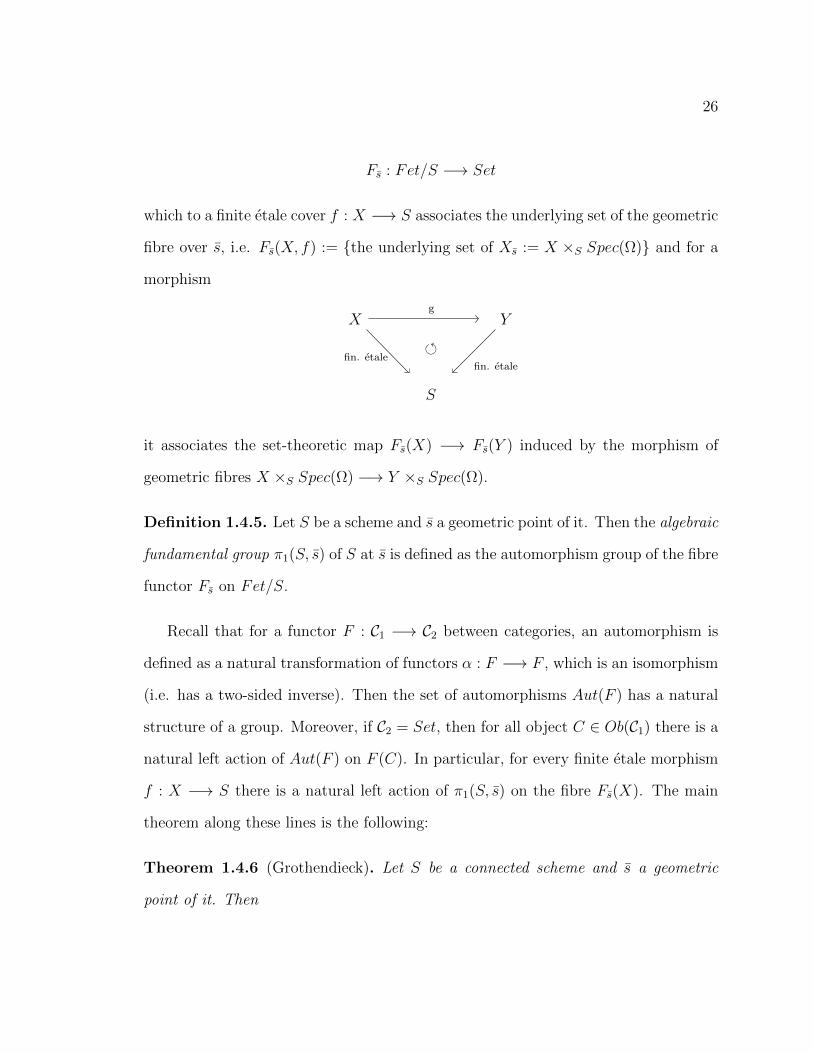
fibre over s, i.e. Fs(X, f) := the underlying set of Xs := X ×S Spec(Ω) and for a

morphism

X Y

S

g

fin. etalefin. etale

it associates the set-theoretic map Fs(X) −→ Fs(Y ) induced by the morphism of

geometric fibres X ×S Spec(Ω) −→ Y ×S Spec(Ω).

Definition 1.4.5. Let S be a scheme and s a geometric point of it. Then the algebraic

fundamental group π1(S, s) of S at s is defined as the automorphism group of the fibre

functor Fs on Fet/S.

Recall that for a functor F : C1 −→ C2 between categories, an automorphism is

defined as a natural transformation of functors α : F −→ F , which is an isomorphism

(i.e. has a two-sided inverse). Then the set of automorphisms Aut(F ) has a natural

structure of a group. Moreover, if C2 = Set, then for all object C ∈ Ob(C1) there is a

natural left action of Aut(F ) on F (C). In particular, for every finite etale morphism

f : X −→ S there is a natural left action of π1(S, s) on the fibre Fs(X). The main

theorem along these lines is the following:

Theorem 1.4.6 (Grothendieck). Let S be a connected scheme and s a geometric

point of it. Then

27

• the group π1(S, s) is profinite and its action on Fs(X) is continous for every X

in Fet/S.

• The fibre functor Fs induces an equivalence of the category Fet/S with the

category of finite continous left π1(S, s)-sets. Connected covers corresponds to

sets with transitive action, and Galois covers to finite quotients of π1(S, s).

Proof. Theorem 5.4.2 in [Sza09b].

This is a vast generalization of basic Galois Theory, at least in the reformulation

of Grothendieck, namely:

Example 1.4.7. Let S = Spec(k) for a field k. Then by definition a finite etale cover

X of S is the spectrum of a finite etale k-algebra X = Spec(L). For a geometric point

s the fibre functor gives Fs(X) = Spec(L⊗kΩ) (if X is connected), which is the finite

set of k-algebra homomorphisms L −→ Ω (the image of such a morphism lies in the

separable closure ks of k in Ω). So we see that Fs(X) = Homk(L, ks) and hence

π1(S, s) ∼= Gal(ks/k). As Spec(ks) is not a finite etale cover of Spec(k), the functor

is not representable by Spec(ks), but it is pro-representable. For more details see

section 5.4 in [Sza09b].

We see that we need to fix a geometric point s for defining the algebraic funda-

mental group of S. But just as in topology, algebraic fundamental groups of a scheme

S defined at different base points are non-canonically isomorphic:

Proposition 1.4.8. For a connected scheme S and two different geometric points

s, s′

of it, there exists an isomorphism of fibre functors α : Fs∼=−→ Fs′ , hence there

exists a continous isomorphism of profinite groups π1(S, s)∼=−→ π1(S, s

′).

28

Proof. For the existence of an isomorphism of fibre functors see Proposition 5.5.1 in

[Sza09b]. Such an isomorphism is called a path between the geometric points s and

s′. Then an isomorphism α : Fs

∼=−→ Fs′ of the fibre functors induces an isomorphism

of their automorphism group via ϕ 7→ α−1 ϕ α.

In particular

Corollary 1.4.9. The isomorphism π1(S, s)∼=−→ π1(S, s

′) induced by a path depends

on the path but it is unique up to an inner automorphism of π1(S, s) or π1(S, s′)

respectively. In particular the maximal abelian quotient of π1(S, s) is independent of

the choice of a geometric point and hence denoted by πab1 (S).

Next we investigate functoriality. Let S and T be connected schemes with geo-

metric points s : Spec(Ω) −→ S and t : Spec(Ω) −→ T respectively, together with a

morphism ϕ : S −→ T preserving base points, i.e. t = ϕ s. Then we have a base

change functor

BS,T : Fet/T −→ Fet/S

by associating to each object X −→ T in Fet/T the base change S ×T X in Fet/S

and to a morphism X −→ Y in Fet/T the induced morphism S ×T X −→ S ×T Y

in Fet/S. The base point preserving property gives an equality of functors

Ft = Fs BS,T

hence every automorphism of the fibre functor Fs induces an automorphism of the

fibre functor Ft giving the induced map on the algebraic fundamental groups

ϕ∗ : π1(S, s) −→ π1(T, t)

29

which is a continuous homomorphism of profinite groups.

Proposition 1.4.10. The induced map ϕ∗ is surjective if and only if for every con-

nected finite etale cover X −→ T the base change S ×T X −→ S is connected as

well.

Proof. Proposition 5.5.4 in [Sza09b].

Now we state the very important homotopy exact sequence theorem:

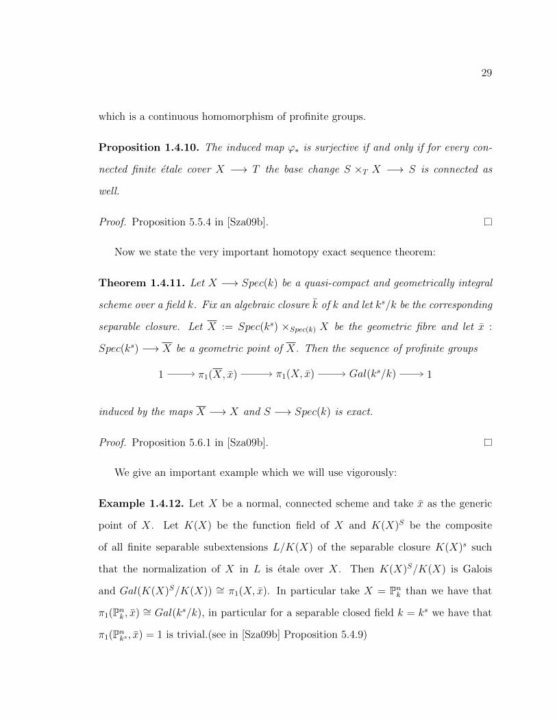
Theorem 1.4.11. Let X −→ Spec(k) be a quasi-compact and geometrically integral

scheme over a field k. Fix an algebraic closure k of k and let ks/k be the corresponding

separable closure. Let X := Spec(ks) ×Spec(k) X be the geometric fibre and let x :

Spec(ks) −→ X be a geometric point of X. Then the sequence of profinite groups

1 π1(X, x) π1(X, x) Gal(ks/k) 1

induced by the maps X −→ X and S −→ Spec(k) is exact.

Proof. Proposition 5.6.1 in [Sza09b].

We give an important example which we will use vigorously:

Example 1.4.12. Let X be a normal, connected scheme and take x as the generic

point of X. Let K(X) be the function field of X and K(X)S be the composite

of all finite separable subextensions L/K(X) of the separable closure K(X)s such

that the normalization of X in L is etale over X. Then K(X)S/K(X) is Galois

and Gal(K(X)S/K(X)) ∼= π1(X, x). In particular take X = Pnk than we have that

π1(Pnk , x) ∼= Gal(ks/k), in particular for a separable closed field k = ks we have that

π1(Pnks , x) = 1 is trivial.(see in [Sza09b] Proposition 5.4.9)

30

Finally we give a relative version of the above homotopy exact sequence:

Theorem 1.4.13. Let f : X −→ S be a proper, surjective morphism of finite pre-

sentation with geometrically connected fibres. Let s : Spec(Ω) −→ S be a geometric

point of S such that Ω is the algebraic closure of the residue field of the image of s in

S, and let x be a geometric point of the fibre Xs := Spec(Ω)×SX. Then the sequence

π1(Xs, x) π1(X, x) π1(S, s) 1

is exact.

Proof. This is Corollaire 6.11, Expose IX. in [Gro61].

31

1.5 l-adic Local Systems and Representations

In this section we will define l-adic sheaves and study some of their basic properties,

especially concentrating on l-adic local systems. Then we will investigate the rela-

tionship between l-adic local systems on a connected scheme X and continous l-adic

representations of its etale fundamental group and give the correspondence appear-

ing in the left vertical side of diagram 1.1.2. The main references for this section are

Expose VI. in [Gro66], [Shi05] and § 12. in [FK88].

Let X be a connected scheme and Xet its etale site, i.e. the underlying category

is Et/X whose objects are the etale morphisms U −→ X and whose arrows are

the morphisms ϕ : U −→ V over X together with the Grothendieck topology whose

coverings are the surjective families of morphisms (Ui −→ U)i∈I in Et/X. We fix also

a prime number l invertible on X.

Definition 1.5.1. An etale sheaf F on X (or a sheaf on Xet) is a contravariant

functor

F : Et/X −→ Set or (Ab, . . . )

such that

F(U)→∏

i∈I F(Ui) ⇒∏

i,j∈I F(Ui ×U Uj)

is an equalizer diagram for every object U −→ X in Et/X and for every etale covering

(Ui −→ U)i∈I .

An etale sheaf F on X is called

1. local constant if there is a covering (Ui −→ X)i∈I such that the restrictions F|Ui

are constant etale sheaves for all i ∈ I;

32

2. constructible if for every closed immersion j : Z −→ X there exists an open

subset U ⊂ Z such that the etale sheaf j−1F|U is locally constant having finite

stalks.

In particular for a smooth, geometrically irreducible curve C over a field k an etale

sheaf F is constructible if it has finite stalks and there exists an open subset U ⊂ C

such that F|U is locally constant.

Also for a connected scheme X there is an equivalence between the category of

finite etale coverings Fet/X and the category of locally constant etale sheaves with

finite stalks (Proposition 6.16 in [Mil08c]).

Definition 1.5.2. A sheaf of Zl-modules F on X is an inverse system

(Fn, fn+1 : Fn+1 −→ Fn)n∈N

such that

1. for all n ∈ N, Fn is a constructible sheaf of Z/lnZ-modules;

2. for all n ∈ N the map fn+1 : Fn+1 −→ Fn induces an isomorphism

Fn+1 ⊗Z/ln+1Z Z/lnZ ∼= Fn.

Definition 1.5.3. A sheaf of Zl-modules F on X is called locally constant if each Fn

is locally constant.

We can extend the previous definitions by passing to a finite field extension K/Ql,

where denote by OK and mK resp. the valuation ring of K and its maximal ideal.

Then we make the exact same definitions

Definition 1.5.4. A sheaf of OK-modules F on X is an inverse system

33

(Fn, fn+1 : Fn+1 −→ Fn)n∈N

such that

1. for all n ∈ N, Fn is a constructible sheaf of OK/mn-modules;

2. for all n ∈ N the map fn+1 : Fn+1 −→ Fn induces an isomorphism

Fn+1 ⊗OK/mn+1 OK/mn ∼= Fn.

Definition 1.5.5. A sheaf of OK-modules F on X is called locally constant if each

Fn is locally constant.

The morphisms HomOK−sheaves(F,G) between sheaves of OK-modules are defined

as the compatible systems of morphisms of sheaves of OK/mn-modules for all n ∈ N

giving an OK-module structure to HomOK−sheaves(F,G).

Then for each finite field extension K/Ql we define the category of K-sheaves,

whose objects are the sheaves of OK-modules and the morphisms are defined by

HomK−sheaves(F,G) := HomOK−sheaves(F,G)⊗OK K.

(We will sometimes use the notation FK for the image of a sheaf of OK-modules F in

the category of K-sheaves.)

If K runs through all the finite extensions of Ql, the categories of K-sheaves form

a directed system, as for all inclusion K ⊂ L an L-sheaf can be considered naturally

as a K-sheaf as well, so we take the direct limit obtaining the category of Ql-sheaves.

Definition 1.5.6. Let F be a sheaf of OK-modules on X. Then the K-sheaf FK

is said to be locally constant, if the sheaf of OK-modules F is locally constant. A

Ql-sheaf F on X is called locally constant if it is a direct limit of locally constant

K-sheaves.

34

Finally we arrived to our first main object:

Definition 1.5.7. An l-adic local system L on X is a locally constant Ql-sheaf on

X.

We can define stalks for l-adic local systems.

Definition 1.5.8. Let X be a connected scheme, L a sheaf of OK-modules on X and

s : Spec(Ω) −→ X a geometric point. Then we define the stalk to be

Ls := lim←−n∈N(Ln)s

where (Ln)s are the etale stalks (II.2. in [Mil80]). For a K-sheaf LK we define the

stalk to be

LKs := Ls ⊗OK K.

To define the stalk of a Ql-sheaf we just take the direct limit of the stalks of the

K-sheaves defining the Ql-sheaf.

For a locally constant Ql-sheaf L on a connected scheme X the stalk Ls is a finite

dimensional Ql-vector space whose dimension is called the rank of the l-adic local

system L.

An etale sheaf F on X is said to be representable if it is representable by an etale

covering U −→ X in Et/X

F(−) = HomX(−, U).

Constant etale sheaves are representable (Chapter 6 in [Mil08c]), hence locally con-

stant (constructible) etale sheaves are also representable by an etale covering U −→ X

(3.18 Lemma in [FK88]). For a geometric point s : Spec(Ω) −→ X the fibre Us =

35

U×XSpec(Ω) is canonically isomorphic to the stalk Fs and by definition has a natural

continuous left action % : π1(X, s)× Fs −→ Fs. By Theorem 1.4.6 we get

Proposition 1.5.9. The assignment F 7→ (Fs, %) establishes an equivalence between

the category of locally constant (constructible) etale sheaves of abelian groups and the

category of finite continuous π1(X, s)-modules.

Proof. A I.7 Proposition in [FK88].

By passing to the projective limits we get the main result we are seeking for

Theorem 1.5.10. The assignment L 7→ (Ls, %) establishes an equivalence between the

category of locally constant sheaves of Zl-modules and the category of finitely generated

Zl-modules on which π1(X, s) acts continuously with respect to the l-adic topology.

For a locally constant Ql-sheaf LQl there is a continuous action of π1(X, s) on

the stalk LQls = Ls ⊗Zl Ql. Then the functor LQl 7→ LQl

s establishes an equivalence

between the category of locally constant Ql-sheaves and the category of continuous

representations of π1(X, s) on finite dimensional vector spaces over Ql.

Proof. A I.8 Proposition in [FK88] and Expose VI., Proposition 1.2.5 in [Gro66].

The theorem remains true word by word if we pass to locally constant K-sheaves

and hence also for l-adic local systems.

Specializing to our situation let C be a smooth projective, geometrically irre-

ducible curve over a finite field k, l a prime number different from char(k) = p and

s : Spec(Ω) −→ C a geometric point. Let L be a 1-dimensional l-adic local sys-

tem on C, hence the fibre Ls is a 1-dimensional vector space over Ql. Let us fix

36

an isomorphism ϕ : Ls ∼= Ql. Then the action of π1(C, s) on Ls will be a continu-

ous 1-dimensional l-adic representation χ : π1(C, s) → Q∗l , which necessarily factors

through the maximal abelian quotient πab1 (C) (see Corollary 1.4.9 for notation).

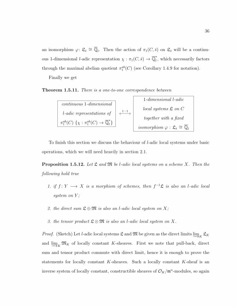
Finally we get

Theorem 1.5.11. There is a one-to-one correspondence between

continuous 1-dimensional

l-adic representations of

πab1 (C) χ : πab1 (C) → Q∗l

1-dimensional l-adic

local systems L on C

together with a fixed

isomorphism ϕ : Ls ∼= Ql

1 : 1

To finish this section we discuss the behaviour of l-adic local systems under basic

operations, which we will need heavily in section 2.1.

Proposition 1.5.12. Let L and M be l-adic local systems on a scheme X. Then the

following hold true

1. if f : Y −→ X is a morphism of schemes, then f−1L is also an l-adic local

system on Y ;

2. the direct sum L⊕M is also an l-adic local system on X;

3. the tensor product L⊗M is also an l-adic local system on X.

Proof. (Sketch) Let l-adic local systems L and M be given as the direct limits lim−→KLK

and lim−→KMK of locally constant K-sheaves. First we note that pull-back, direct

sum and tensor product commute with direct limit, hence it is enough to prove the

statements for locally constant K-sheaves. Such a locally constant K-sheaf is an

inverse system of locally constant, constructible sheaves of OK/mn-modules, so again

37

we can restrict ourselves to prove the statements for ”ordinary” locally constant,

constructible etale sheaves.

So let F be a locally constant etale sheaf on X. Then there exists an etale covering

(Ui −→ X)i∈I such that F|Ui is constant. As pull-backs of constant etale sheaves are

obviously constant, we get that f−1F is constant on Y ×X Ui, hence locally constant

on Y . Let G be another locally constant etale sheaf on X such that it is constant on

the etale covering (Vj −→ X)j∈J . As the direct sum and tensor product of constant

sheaves are constant, the direct sum F ⊕ G and the tensor product F ⊗ G will be

constant on the etale covering (Ui ×X Vj −→ X)i∈I,j∈J , hence locally constant on X.

Finally let F and G be constructible etale sheaves on X, i.e. for every closed

immersion j : Z → X there exists open subsets U ⊂ Z and V ⊂ Z such that the

restrictions F|U and G|V are locally constant on U and V resp. We can reduce to

the case that X is irreducible. Then using the above arguments we see that on the

open subset U ×Z V ⊂ Z the direct sum F ⊕ G and the tensor product F ⊗ G will

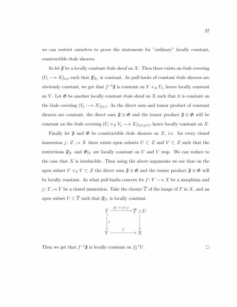
be locally constant. As what pull-backs concern let f : Y −→ X be a morphism and

j : T → Y be a closed immersion. Take the closure T of the image of T in X, and an

open subset U ⊂ T such that F|U is locally constant.

T T ⊃ U

Y X

fT := f j

j

f

Then we get that f−1F is locally constant on f−1T U .

38

1.6 The Faisceaux-Fonctions Correspondence

In this section we will discuss Grothendieck’s function-sheaf correspondence and make

major steps toward establishing the connection appearing in the right vertical side

of diagram 1.1.2, which will be accomplished in section 2.2. The main references are

[Sommes trig.] in [Del77], [Gai04] and [Shi05].

First we need to define the Frobenius action on local systems.

Definition 1.6.1 (construction of the Frobenius action). Let X be a connected

scheme over a finite field k = Fq and L be an l-adic local system of rank r on

X. Let x : Spec(Fqn) −→ X be a closed point and x : Spec(Fq) −→ X a geometric

point lying above it. Then we have isomorphisms

Qr

l∼= Lx ∼= x−1L

where the last space is a discrete Gal(Fq/Fqn)-module by Chapter II., Theorem 1.9

in [Mil80]. The automorphism in Gal(Fq/Fqn) defined by

Frobn : x 7→ xqn

is called the nth power of the arithmetic Frobenius and it defines an automorphism

of the r-dimensional Ql-vector space Lx denoted by Frobx. This whole construction

depends on the choice of a geometric point and hence only well-defined up to inner

automorphism by Corollary 1.4.9, but the trace of the Frobenius is a well-defined

element in Ql and denoted by trL(Frobx).

Let G be a connected, separated, commutative group scheme of finite type defined

over a finite field k = Fq. As usual let l be a prime number different from char(k) = p

and denote by m : G×G −→ G, i : G −→ G and e : Spec(k) −→ G the multiplication

39

map, the inverse map and the identity map respectively, where the image of the

identity will be also denoted by 0 ∈ G.

Definition 1.6.2. An l-adic character sheaf L on G is a 1-dimensional l-adic local

system on G together with a trivialization L0∼= Ql satisfying m−1L ∼= L L.

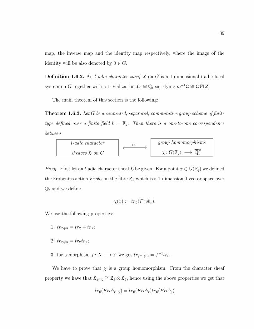
The main theorem of this section is the following:

Theorem 1.6.3. Let G be a connected, separated, commutative group scheme of finite

type defined over a finite field k = Fq. Then there is a one-to-one correspondence

between

l-adic character

sheaves L on G

group homomorphisms

χ : G(Fq) −→ Q×l

1 : 1

Proof. First let an l-adic character sheaf L be given. For a point x ∈ G(Fq) we defined

the Frobenius action Frobx on the fibre Lx which is a 1-dimensional vector space over

Ql and we define

χ(x) := trL(Frobx).

We use the following properties:

1. trL⊕K = trL + trK;

2. trL⊗K = trLtrK;

3. for a morphism f : X −→ Y we get trf−1(L) = f−1trL.

We have to prove that χ is a group homomorphism. From the character sheaf

property we have that Lx+y∼= Lx⊗Ly, hence using the above properties we get that

trL(Frobx+y) = trL(Frobx)trL(Froby)

40

that is χ(x+ y) = χ(x)χ(y).

(⇐) First we define the absolute Frobenius.

Definition 1.6.4. Let G be a connected group scheme defined over a finite field

k = Fq. The absolute Frobenius is the scheme morphism over Spec(Fq)

Frq : (G,OG) −→ (G,OG)

defined as the identity map on the underlying topological space and as g 7→ gq on the

structure sheaf of rings OG.

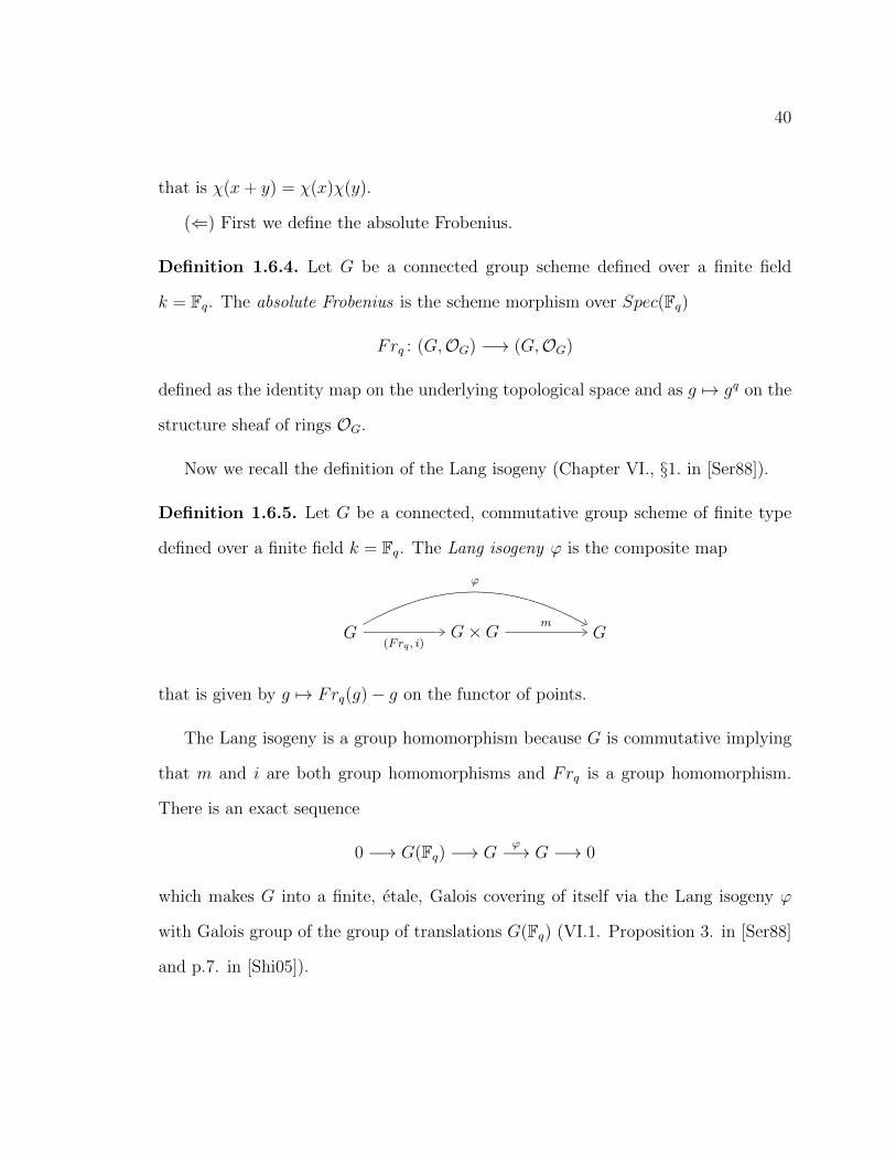
Now we recall the definition of the Lang isogeny (Chapter VI., §1. in [Ser88]).

Definition 1.6.5. Let G be a connected, commutative group scheme of finite type

defined over a finite field k = Fq. The Lang isogeny ϕ is the composite map

G G×G G(Frq , i)

m

ϕ

that is given by g 7→ Frq(g)− g on the functor of points.

The Lang isogeny is a group homomorphism because G is commutative implying

that m and i are both group homomorphisms and Frq is a group homomorphism.

There is an exact sequence

0 −→ G(Fq) −→ Gϕ−→ G −→ 0

which makes G into a finite, etale, Galois covering of itself via the Lang isogeny ϕ

with Galois group of the group of translations G(Fq) (VI.1. Proposition 3. in [Ser88]

and p.7. in [Shi05]).

41

Now let a group homomorphism χ : G(Fq) −→ Q×l be given. Then first to give

a 1-dimensional l-adic local system L on G is the same as giving a continuous, 1-

dimensional l-adic representation πab1 (G) −→ Q×l (section 1.5). But as ϕ : G −→ G

is a finite, etale, Galois covering with Galois group G(Fq), there exists a natural

surjection

ψ : πab1 (G) G(Fq)

by Example 1.4.12. The composite map χψ : πab1 (G) −→ Q×l gives us a 1-dimensional

l-adic local system L on G. Note that by construction ϕ−1L is a constant Ql-sheaf, as

to ϕ−1L corresponds the trivial l-adic representation by the above Lang isogeny exact

sequence. We have to prove that L satisfies the character sheaf property m−1L ∼=

L L. For that we consider the following commutative diagram

G×G G

G×G G

m

(ϕ,ϕ)

m

ϕ

The commutativity is ensured by the fact that the absolute Frobenius commutes

with arbitrary morphisms (cf. 3.2.4 Lemma 2.22 in [Liu02]). As ϕ−1L is a constant

Ql-sheaf on G, then

m−1ϕ−1L = (ϕ, ϕ)−1m−1L

is also a constant Ql-sheaf on G×G. Similarly

ϕ−1L ϕ−1L = (ϕ, ϕ)−1L L

is a constant Ql-sheaf on G × G. So to prove the character sheaf property we only

need to show that the Galois group G(Fq)×G(Fq) of G×G (ϕ,ϕ)−→ G×G acts on the

42

same way on the sheaves (ϕ, ϕ)−1m−1L and (ϕ, ϕ)−1L L. For that it is enough to

check the action on the stalks at the geometric point (0, 0) lying over (0, 0). These

stalks are the same as the stalks of m−1L and L L at (0, 0). We have also that

m−1L(0,0)∼= L0. So let (g, h) ∈ G(Fq) × G(Fq) be given. The action of (g, h) is

transformed via m to the action of g+ h ∈ G(Fq) by the commutativity of the above

diagram. But the action of g + h is just multiplication by χ(g + h). Also by similar

arguments the action of (g, h) on LL is given by multiplication by χ(g)χ(h). Hence

(g, h) acts both on m−1L and L L by multiplication by χ(g + h) = χ(g)χ(h), as

wanted.

These two constructions are inverses to each other completing the proof of the

Theorem.

We will use this result in section 2.2 applying to the Picard scheme Pic0C of degree

0 finishing the proof of the connection appearing in the right vertical side of diagram

1.1.2.

Chapter 2

The Proof of the Main Theorem ofthe Unramified Theory

In this chapter we will begin with final preliminary works proving the correspondences

appearing in diagram 1.1.2 and after that we will give Deligne’s geometric proof of

the Main Theorem 1.1.4.

2.1 Preliminary Constructions

Let C be a smooth, projective, geometrically irreducible curve of genus g over a finite

field k = Fq. Let us begin with building up the connection between 1-dimensional

l-adic local systems on the curve C and 1-dimensional l-adic local systems on the

Picard scheme PicC appearing in the bottom row of diagram 1.1.2.

So let L be a 1-dimensional l-adic local system on C. We will construct a 1-

dimensional l-adic local system L(d) on C(d) using the following construction. First

we define the l-adic local system Ld on Cd by

Ld :=⊗d

i=1 pr−1i L

43

44

using the natural projections pri : Cd → C for i = 1, 2, . . . , d. This is an l-adic

local system by Proposition 1.5.12. Next we want to analyze the stalks of this l-

adic local system. To do this, we can restrict ourselves to the case of locally constant,

constructible etale sheaves using the reduction argument in Proposition 1.5.12. Hence

in the following we assume that L is a locally constant, constructible etale sheaf of

rank 1.1

Now by definition we have that the stalk at a geometric point p = (p1, p2, . . . , pd) ∈

Cd is

(Ld)p =⊗d

i=1 Lpi .

Also we have that for a σ ∈ Sd the stalk at σp = (pσ(1), pσ(2), . . . , pσ(d)) is

(Ld)σp =⊗d

i=1 Lpσ(i) .

But we have an isomorphism

ψp,σ :⊗d

i=1 Lpi∼=−→

⊗di=1 Lpσ(i)

by the commutativity of tensor product. This means that Ld is an Sd-equivariant

locally constant etale sheaf on Cd.

Now we need to descend to the quotient C(d) and investigate how sheaves behave:

Proposition 2.1.1. Let L be a locally constant etale sheaf of rank 1 on C and con-

sider the symmetrization morphism π : Cd → C(d) for an integer d ≥ 1. Then the

etale sheaf L(d) := (π∗Ld)Sd of Sd-invariants of the push-forward of Ld is a locally

constant etale sheaf of rank 1 on C(d).

1Of course Proposition 1.5.12 holds true a fortiori in that case.

45

Proof. First we note that in general for a morphism f : X → Y of schemes and an

etale sheaf F on X there is a natural morphism f−1f∗F → F. If a finite group G

acts on X and the sheaf F is G-equivariant then there is a natural action of G on

the push-forward f∗F. Hence the inclusion of sheaves (f∗F)G → f∗F on Y induces a

morphism of sheaves f−1(f∗F)G → f−1f∗F on X such that the composition

f−1(f∗F)G f−1f∗F F

gives us a morphism of sheaves f−1(f∗F)G → F on X. Now in the case of our

proposition we have

Claim 2.1.2. The natural morphism of etale sheaves π−1(π∗Ld)Sd → Ld on Cd is

an isomorphism.

Proof. To prove the claim first we consider the stalks of the etale sheaves π∗Ld

and (π∗Ld)Sd on C(d). As the symmetrization morphism is a finite, hence proper,

surjective map, we can assume that a geometric point in C(d) is given by

π(p) := π((p1, p2, . . . , pd)) ∈ C(d)

where p is a geometric point of Cd. Then it follows that

π−1π(p) = Sd p = (pσ(1), pσ(2), . . . , pσ(d)| σ ∈ Sd)

i.e. the orbit of p under the action of Sd. Now consider the following commutative

diagram:

46

π−1π(p) Cd

π(p) C(d)

j′

π′

j

π

where the j and j′

are the inclusion maps and π′

is the first projection of the fibre

product. By the Proper Base Change Theorem (Theorem 17.10 in [Mil08c]) we have

a canonical isomorphism

j−1π∗Ld

∼=−→ π′∗(j

′)−1Ld.

Now we will use the following theorem:

Theorem 2.1.3. Let π : X −→ Y be a morphism of schemes.

For any etale sheaf F on Y and any geometric point x ∈ X we have

(π−1F)x ∼= Fπ(x).

If π : X −→ Y is a finite morphism and G is an etale sheaf on X, then for any

geometric point y ∈ Y we have

(π∗G)y =∏

π(x)=yGx.

Proof. The first statement (a) is proved in Ch.II.Theorem 3.2.(a) in [Mil80]. The

second statement (b) is proved in Ch.II.Corollary 3.5.(c) in [Mil80].

By this theorem we have that

j−1π∗Ld = (π∗L

d)π(p)

and also that

π′∗(j

′)−1Ld =

∏p′∈Sdp(L

d)p′ .

47

If p′

= (p′1, p

′2, . . . , p

′

d) ∈ Sd p then using the property of external tensor products

above we have that

(π∗Ld)π(p) =

∏p′∈Sdp

⊗di=1 Lp′i

.

A permutation σ ∈ Sd acts on the stalk in the following way:

σ(π∗Ld)π(p) =

∏p′∈Sdp

⊗di=1 Lp′

σ(i)

hence we get for the Sd-invariants

(π∗Ld)Sdπ(p)

∼=⊗d

i=1 Lpi .

Using again the property of the pull-back on stalks (Theorem 2.1.3 (a)) we have for

any p′ ∈ π−1π(p) that

π−1((π∗Ld)Sd)p′ = (π∗L

d)Sdπ(p)

which is

π−1((π∗Ld)Sd)p′ =

⊗di=1 Lpi

∼= Ldp′

hence these isomorphisms on the stalks induce an isomorphism between the etale

sheaves on Cd

π−1(L(d))∼=−→ Ld

completing the proof of the claim.

It remained to prove that L(d) is a locally constant etale sheaf on C(d). We note

that Ld being locally constant is representable by an etale covering. Then as the

push-forward and a subsheaf of a representable sheaf is representable, we get that at

least L(d) is representable by a scheme Z on C(d). By Theorem 2.1.3 (a) we know that

for any geometric point π(p) ∈ C(d) the stalks are isomorphic π−1(L(d))p∼=−→ L

(d)π(p).

48

Hence there exists an etale neighborhood U of π(p) and a section s : U −→ Z which

generates the stalk L(d)π(p). The pull-back of this section must generate all stalks of

π−1(L(d)) in an etale neighborhood of p ∈ Cd, as π−1(L(d)) is a locally constant etale

sheaf on Cd. As the stalks of the sheaf L(d) are 1-dimensional and the pull-back of

the section generates the stalks π−1(L(d))p in some etale neighborhood, it follows that

the section must generate the stalks L(d)π(p) in some etale neighborhood of π(p) as well,

i.e. the sheaf L(d) becomes constant on an etale covering. This completes the proof

of the Proposition.

Recall that in section 1.3 we have defined the Abel-Jacobi natural transformation

of the functors DivdC and PicdC for an integer d ≥ 1 and indicated also that we can

assume that C has a k-rational point, consequently the functors are representable

inducing a morphism of schemes (using the same notation for the Picard scheme)

AJd : C(d) −→ PicdC

such that on the geometric points the fibre of the Abel-Jacobi map over the class of

an invertible sheaf G of degree d on C is isomorphic to

AJ−1d ([G]) ∼= PH0(C,G)

by Proposition 1.2.6.

It follows that PH0(C,G) 6= ∅ if and only if h0(C,G) := dimkH0(C,G) ≥ 1. By

the Riemann-Roch Theorem we have that

h0(C,G)− h0(C, ωC ⊗ G−1) = d− g + 1

hence our condition is equivalent to

49

h0(C, ωC ⊗ G−1) + d− g ≥ 0.

This is certainly the case if d ≥ g. But we can say more:

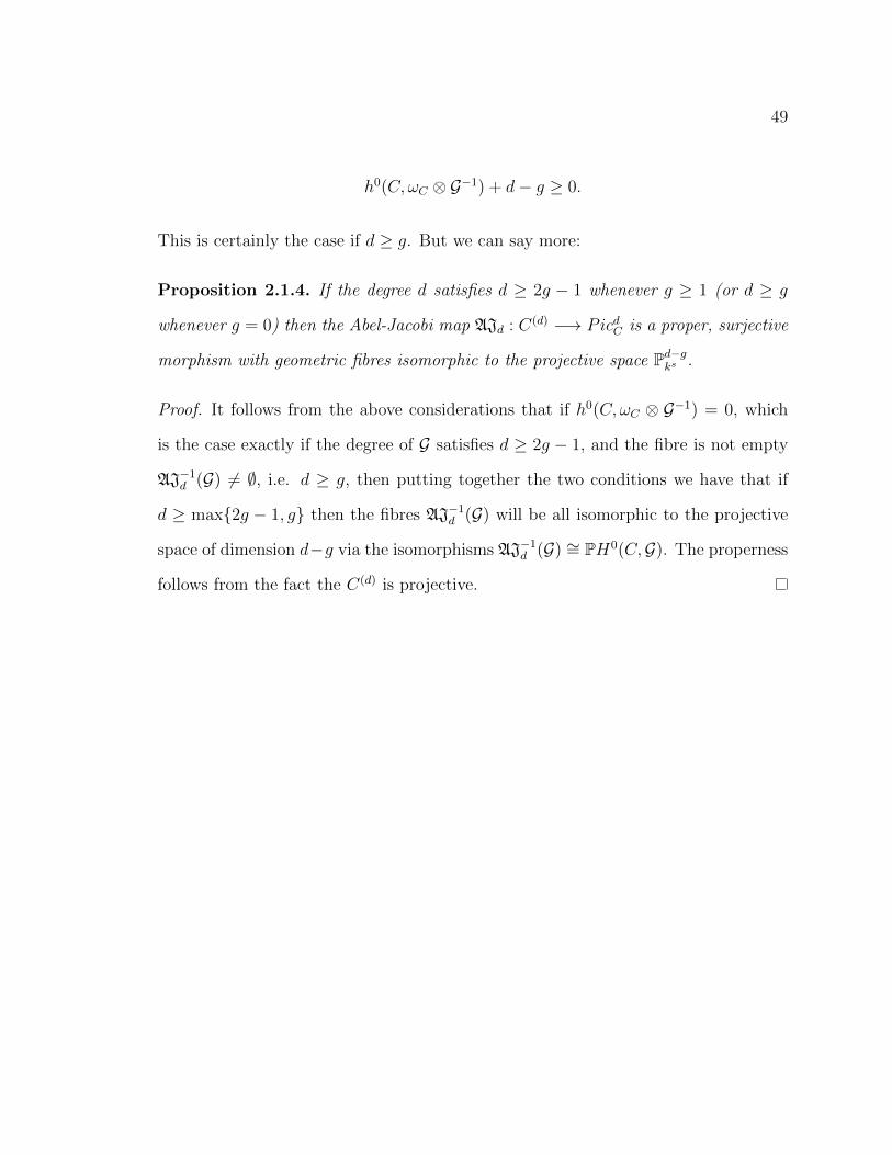
Proposition 2.1.4. If the degree d satisfies d ≥ 2g − 1 whenever g ≥ 1 (or d ≥ g

whenever g = 0) then the Abel-Jacobi map AJd : C(d) −→ PicdC is a proper, surjective

morphism with geometric fibres isomorphic to the projective space Pd−gks .

Proof. It follows from the above considerations that if h0(C, ωC ⊗ G−1) = 0, which

is the case exactly if the degree of G satisfies d ≥ 2g − 1, and the fibre is not empty

AJ−1d (G) 6= ∅, i.e. d ≥ g, then putting together the two conditions we have that if

d ≥ max2g − 1, g then the fibres AJ−1d (G) will be all isomorphic to the projective

space of dimension d−g via the isomorphisms AJ−1d (G) ∼= PH0(C,G). The properness

follows from the fact the C(d) is projective.

50

2.2 Deligne’s Geometric Proof

In this section we turn to the proof of the Main Theorem 1.1.4 using a geometric

argument of Deligne. The main references are [Lau90], [Hei07] and [Hei04].

First we prove

Theorem 2.2.1. (Deligne’s Theorem): There is a one-to-one correspondence between

1-dimensional l-adic

local systems L on C

together with a fixed

isomorphism ϕ : Ls ∼= Ql

1-dimensional l-adic

local systems AL on

PicC together with

a fixed isomorphism

ψ : AL|0 ∼= Ql satisfying

m−1Ad+eL = AdL AeL

1 : 1

Proof. Let be given a 1-dimensional l-adic local system L on C with a fixed iso-

morphism ϕ : Ls ∼= Ql where s : Spec(Ω) −→ C is a geometric point. Then for an

integer d ≥ 1 we constructed a 1-dimensional l-adic local system L(d) := (π∗Ld)Sd

on C(d) in the previous section 2.1. It follows from the correspondence between l-

adic local systems and representations of the fundamental group (section 1.5) that

there is associated to L(d) a unique continuous 1-dimensional l-adic representation

ρL(d) : πab1 (C(d)) −→ Q×l . Now we assume that d ≥ 2g − 1 and apply the relative ho-

motopy exact sequence theorem (1.4.13) to the Abel-Jacobi map AJd : C(d) −→ PicdC

taking into account Proposition 2.1.4 to get the exact sequence

π1(Pd−gks , s) π1(C(d), s) π1(PicdC , s) 1

where ks is the separable closure of the base field k. We know from Example 1.4.12

that π1(Pd−gks , s) = 1 is trivial, hence we get an isomorphism

51

π1(C(d), s) ∼= π1(PicdC , s)

which induces an isomorphism between the abelianized etale fundamental groups

πab1 (C(d)) ∼= πab1 (PicdC).

This means that to the continuous 1-dimensional l-adic representation

ρL(d) : πab1 (C(d)) −→ Q×l

corresponds a unique continuous 1-dimensional l-adic representation

ρAdL : πab1 (PicdC) −→ Q×l

which again corresponds (section 1.5) to a unique 1-dimensional l-adic local system

AdL on PicdC together with a fixed isomorphism ψ : AdL|d0∼= Ql.

For the 1-dimensional l-adic local systems AdL we have the following

Proposition 2.2.2. The 1-dimensional l-adic local systems AdL satisfy

(+)−1Ad+1L = LAdL.

Proof. Let us consider the following commutative diagram

(p,D) (p+D)

C × C(d) C(d+1)

C × PicdC Picd+1C

(p,G) O(p)⊗ G .

+

∼=

id× AJ(d) AJ(d+1)

+

Because of the correspondence between AdL and L(d) constructed above we just have

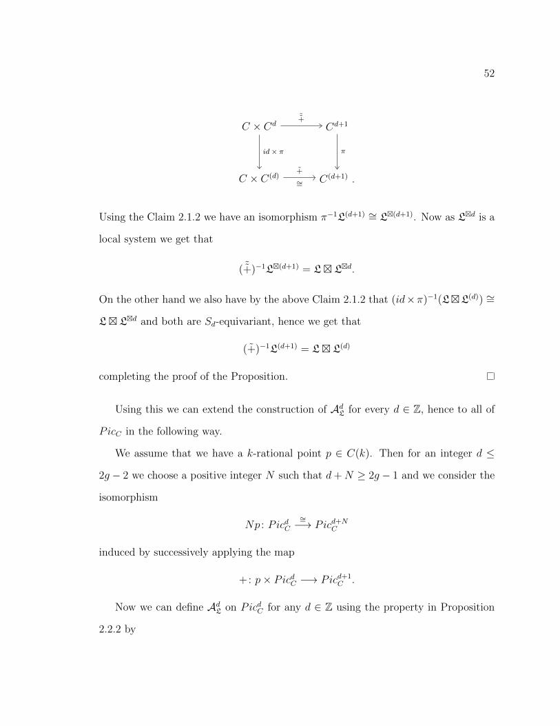
to prove that (+)−1L(d+1) = L L(d). For this we consider the diagram

52

C × Cd Cd+1

C × C(d) C(d+1) .

˜+

id× π

+

∼=

π

Using the Claim 2.1.2 we have an isomorphism π−1L(d+1) ∼= L(d+1). Now as Ld is a

local system we get that

( ˜+)−1L(d+1) = L Ld.

On the other hand we also have by the above Claim 2.1.2 that (id×π)−1(LL(d)) ∼=

L Ld and both are Sd-equivariant, hence we get that

(+)−1L(d+1) = L L(d)

completing the proof of the Proposition.

Using this we can extend the construction of AdL for every d ∈ Z, hence to all of

PicC in the following way.

We assume that we have a k-rational point p ∈ C(k). Then for an integer d ≤

2g − 2 we choose a positive integer N such that d+N ≥ 2g − 1 and we consider the

isomorphism

Np : PicdC∼=−→ Picd+N

C

induced by successively applying the map

+: p× PicdC −→ Picd+1C .

Now we can define AdL on PicdC for any d ∈ Z using the property in Proposition

2.2.2 by

53

AdL := (Np)−1Ad+NL ⊗ L⊗−Np .

We have to prove the multiplicative property of AL, i.e. that for the multiplication

map

m : PicdC × PiceC −→ Picd+eC

defined by

(G,H) 7→ G ⊗H

we have that

m−1Ad+eL∼= AdL AeL.

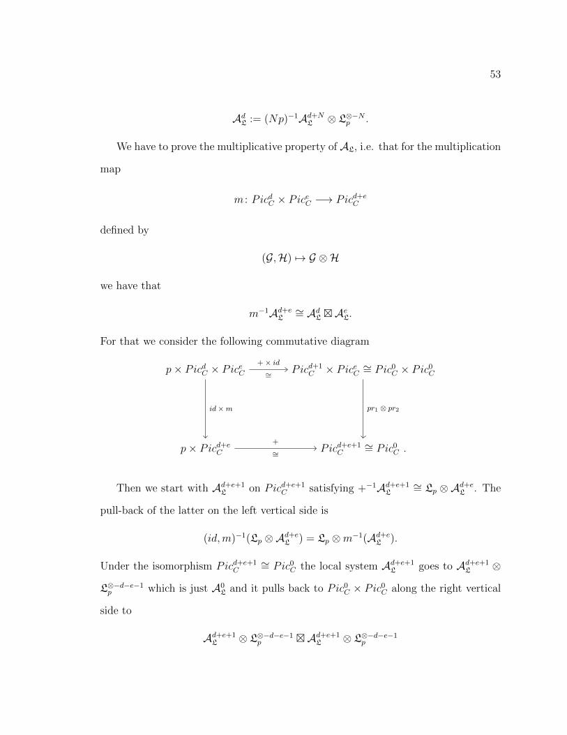
For that we consider the following commutative diagram

p× PicdC × PiceC Picd+1C × PiceC ∼= Pic0

C × Pic0C

p× Picd+eC Picd+e+1

C∼= Pic0

C .

+× id∼=

id×m

+

∼=

pr1 ⊗ pr2

Then we start with Ad+e+1L on Picd+e+1

C satisfying +−1Ad+e+1L

∼= Lp ⊗Ad+eL . The

pull-back of the latter on the left vertical side is

(id,m)−1(Lp ⊗Ad+eL ) = Lp ⊗m−1(Ad+e

L ).

Under the isomorphism Picd+e+1C

∼= Pic0C the local system Ad+e+1

L goes to Ad+e+1L ⊗

L⊗−d−e−1p which is just A0

L and it pulls back to Pic0C × Pic0

C along the right vertical

side to

Ad+e+1L ⊗ L⊗−d−e−1

p Ad+e+1L ⊗ L⊗−d−e−1

p

54

which again goes back under the isomorphism Picd+1C × PiceC ∼= Pic0

C × Pic0C to

Ad+e+1L ⊗ L⊗−ep Ad+e+1

L ⊗ L⊗−d−1p .

Using successively the property +−1Ad+1L∼= Lp ⊗AdL we get

Lp ⊗AdL AeL

hence we get the isomorphism

m−1(Ad+eL ) ∼= AdL AeL.

On the other way round let a rigidified multiplicative 1-dimensional l-adic local

system AL on PicC be given. Then we consider the Abel-Jacobi map

AJ(1) : C −→ Pic1C

and by Proposition 1.5.12 the pull-back

L := AJ−1(1)A1

L

is a 1-dimensional l-adic local system on C together with a rigidification.

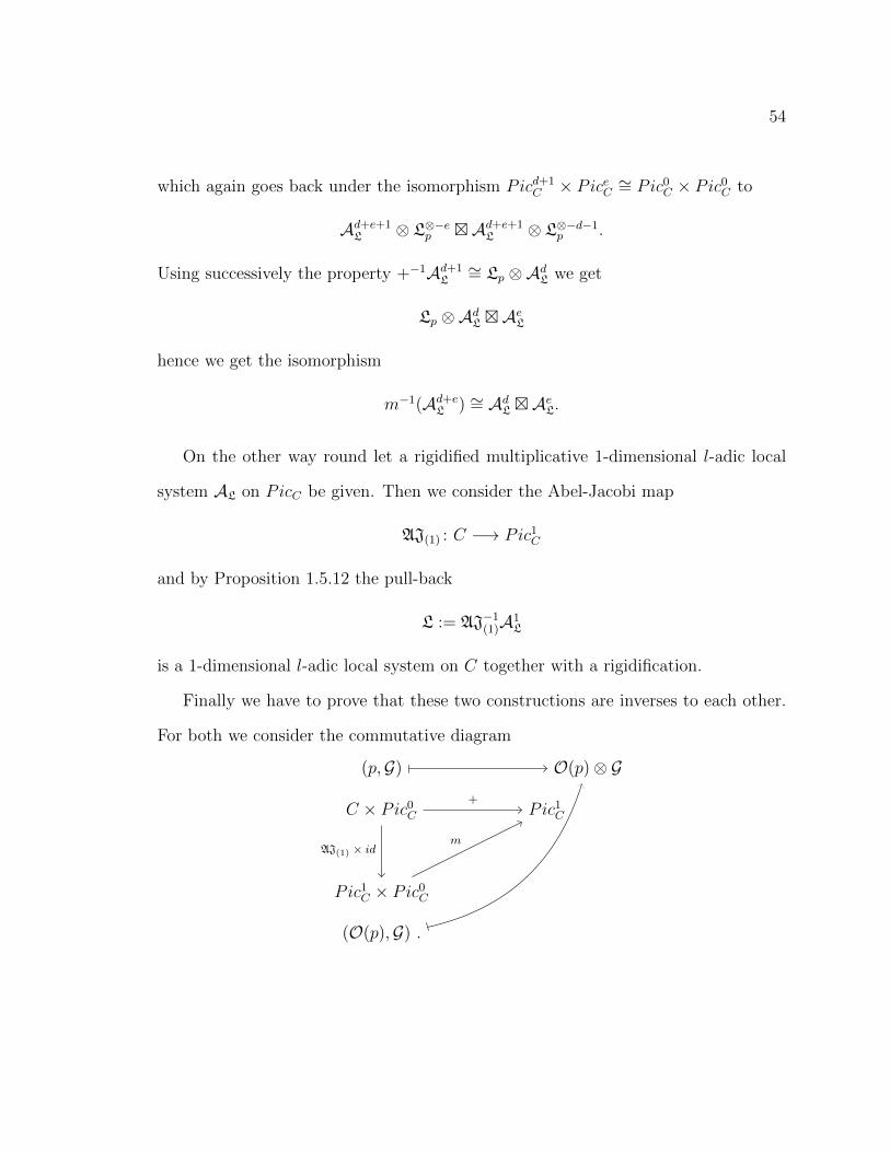
Finally we have to prove that these two constructions are inverses to each other.

For both we consider the commutative diagram

(p,G) O(p)⊗ G

C × Pic0C Pic1

C

Pic1C × Pic0

C

(O(p),G) .

+

AJ(1) × idm

55

Then given a rigidified, 1-dimensional l-adic local system L on C, we can associate

to it a rigidified, multiplicative 1-dimensional l-adic local system AL on PicC , such

that we define L′= AJ−1

(1)A1L. Then using the above diagram

L′A0

L = LA0L A1

L

A1L A0

L

+

AJ(1) × idm

we get L = L′.

Similarly starting with a rigidified, multiplicative 1-dimensional l-adic local system

AL on PicC , we define the rigidified, 1-dimensional l-adic local system L := AJ−1(1)AL

on C. We can associate to it a rigidified, multiplicative 1-dimensional l-adic local

system A′L on PicC . Then using the above diagram

LA0L = L (A′L)0 (A′L)1 = A1

L

A1L A0

L

+

AJ(1) × idm

we get A′L = AL completing the proof of the Theorem.

Next we want to accomplish the proof of the correspondence appearing in the

right vertical side of diagram 1.1.2.

Theorem 2.2.3. There is a one-to-one correspondence between

56

1-dimensional l-adic

representations of Pic0C(k)

χ : Pic0C(k) → Q∗l

together with a Frobenius

action Frobp : Z → Q×l

1-dimensional l-adic

local systems AL on

PicC together with

a fixed isomorphism

ψ : AL|0 ∼= Ql satisfying

m−1Ad+eL∼= AdL AeL

1 : 1

Proof. First let be given a 1-dimensional l-adic local system AL on PicC together

with a fixed isomorphism ψ : AL|0 ∼= Ql satisfying m−1Ad+eL∼= AdL AeL. Then the

restriction A0L on Pic0

C will be a 1-dimensional local system together with a fixed

isomorphism A0L|0 ∼= Ql satisfying the character sheaf property

m−1A0L∼= A0

L A0L

hence by the faisceaux-fonctions correspondence (section 1.6) it will give us a 1-

dimensional l-adic representation of Pic0C(k). Also by Theorem 2.2.1 AL defines a

1-dimensional l-adic local system L on C, hence a sheaf Lp on the point p ∈ C(k),

which is the same as a Frobenius action Frobp : Z −→ Q×l by Definition 1.6.1.

Going on the other way round let be given a 1-dimensional l-adic representation

χ : Pic0C(k) −→ Q×l

together with a Frobenius action Frobp : Z −→ Q×l . Then by Definition 1.6.1 the

Frobenius action defines a sheaf Lp on p ∈ C(k). Also by section 1.6 χ defines a

character sheaf A0χ on Pic0

C together with a fixed trivialization A0χ|0 ∼= Ql. Similarly

as we did in the proof of Deligne’s Theorem we can extend this local system to all of

PicC by

57

Adχ := (−dp)−1A0χ ⊗ Ldp

where −dp is the morphism

−dp := p× PicdC∼=−→ Pic0

C

defined by sending G to G ⊗O(−dp). Using the commutative diagram in the proof of

Theorem 2.2.1 and the argument presented there it follows from this definition that

the 1-dimensional l-adic local system Aχ on PicC will satisfy

m−1Ae+dχ∼= Adχ Aeχ.

These two constructions are inverses to each other completing the proof of the The-

orem.

With this theorem we finally finished the long journey leading to the proof of the

one-to-one correspondences appearing in diagram 1.1.2.

Now we are able to prove Theorem 1.1.4.

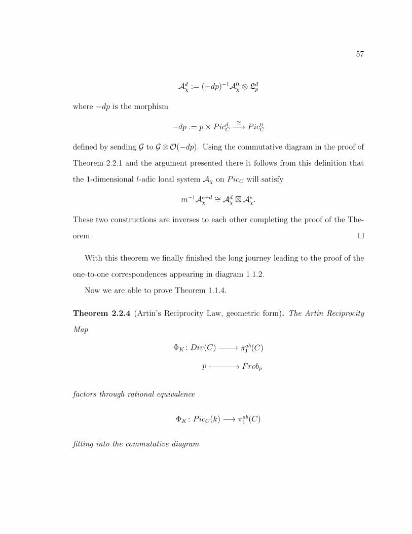
Theorem 2.2.4 (Artin’s Reciprocity Law, geometric form). The Artin Reciprocity

Map

ΦK : Div(C) πab1 (C)

p Frobp

factors through rational equivalence

ΦK : PicC(k) −→ πab1 (C)

fitting into the commutative diagram

58

Pic0C(k) PicC(k) Z

Ker(ϕ) πab1 (C) Z

deg

ϕ

ΦK can (2.2.1)

such that there is an induced isomorphism on the kernels

Pic0C(k) Ker(ϕ) .

∼=

Proof. First we prove that the diagram

Div0(C) Div(C) Z

Ker(ϕ) πab1 (C) Z

deg

ϕ

ΦK can

is commutative. For that we define the maps appearing in the diagram. Let us begin

with the Frobenius element:

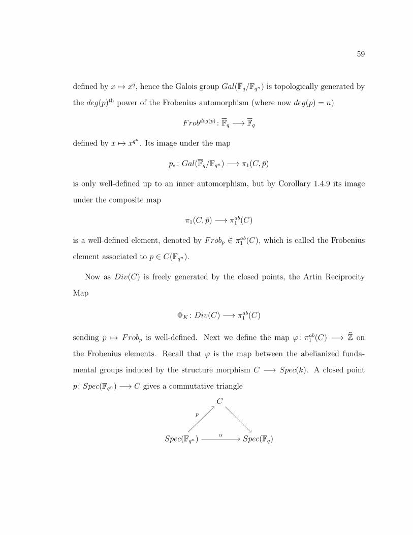
Definition 2.2.5. (construction) Let p : Spec(Fqn) −→ C be a closed point, which

has a degree defined as the degree deg(p) = [k(p) : k] of the field extension k(p)/k,

where k(p) is the residue field of p. We choose a geometric point p : Spec(Fq) −→ C

lying above p. By Example 1.4.7 we have that π1(Spec(Fqn), p) ∼= Gal(Fq/Fqn) hence

the induced map between the etale fundamental groups becomes

p∗ : Gal(Fq/Fqn) −→ π1(C, p).

Now the Galois groupGal(Fq/Fqn) is an open subgroup of the Galois groupGal(Fq/Fq)

which is a profinite group topologically generated by the Frobenius automorphism

Frob : Fq −→ Fq

59

defined by x 7→ xq, hence the Galois group Gal(Fq/Fqn) is topologically generated by

the deg(p)th power of the Frobenius automorphism (where now deg(p) = n)

Frobdeg(p) : Fq −→ Fq

defined by x 7→ xqn. Its image under the map

p∗ : Gal(Fq/Fqn) −→ π1(C, p)

is only well-defined up to an inner automorphism, but by Corollary 1.4.9 its image

under the composite map

π1(C, p) −→ πab1 (C)

is a well-defined element, denoted by Frobp ∈ πab1 (C), which is called the Frobenius

element associated to p ∈ C(Fqn).

Now as Div(C) is freely generated by the closed points, the Artin Reciprocity

Map

ΦK : Div(C) −→ πab1 (C)

sending p 7→ Frobp is well-defined. Next we define the map ϕ : πab1 (C) −→ Z on

the Frobenius elements. Recall that ϕ is the map between the abelianized funda-

mental groups induced by the structure morphism C −→ Spec(k). A closed point

p : Spec(Fqn) −→ C gives a commutative triangle

Spec(Fqn)

C

Spec(Fq)

p

α

60

where the map α is induced by the natural inclusion Fq −→ Fqn , hence the map

between the etale fundamental groups

α∗ : Gal(Fq/Fqn) → Gal(Fq/Fq)

is just the natural inclusion. Then by the functoriality property of the etale funda-

mental group we have that

ϕ(Frobp) = Frobdeg(p).

Moreover this map is surjective by Proposition 1.4.10. The other two maps are defined

by

deg(∑

i dipi) :=∑

i dideg(pi) and can(1) := Frob

where deg is surjective and can is injective.2 Now the commutativity of the diagram

follows from

ϕ(ΦK(p)) = Frobdeg(p) = can(deg(p))

and the fact that by the universal property of the kernel, the Reciprocity Map ΦK

restricted to the divisors Div0(C) of degree 0 factors through Ker(ϕ).

It remained to prove that the Reciprocity Map factors through the principal di-

visors. For that let us take a continuous, 1-dimensional l-adic representation

χ : πab1 (C) −→ Q×l .

By the geometric constructions we carried out and appearing in diagram 1.1.2, we

can associate to χ a 1-dimensional l-adic local system L on C, such that for a closed

point p : Spec(Fqn) −→ C, the Frobenius element Frobp acts on the fibre Lp by

2Hopefully it may not cause any confusion that deg denotes two different maps, as the notationsare so natural in both cases, that the change of notation may have caused more confusion.

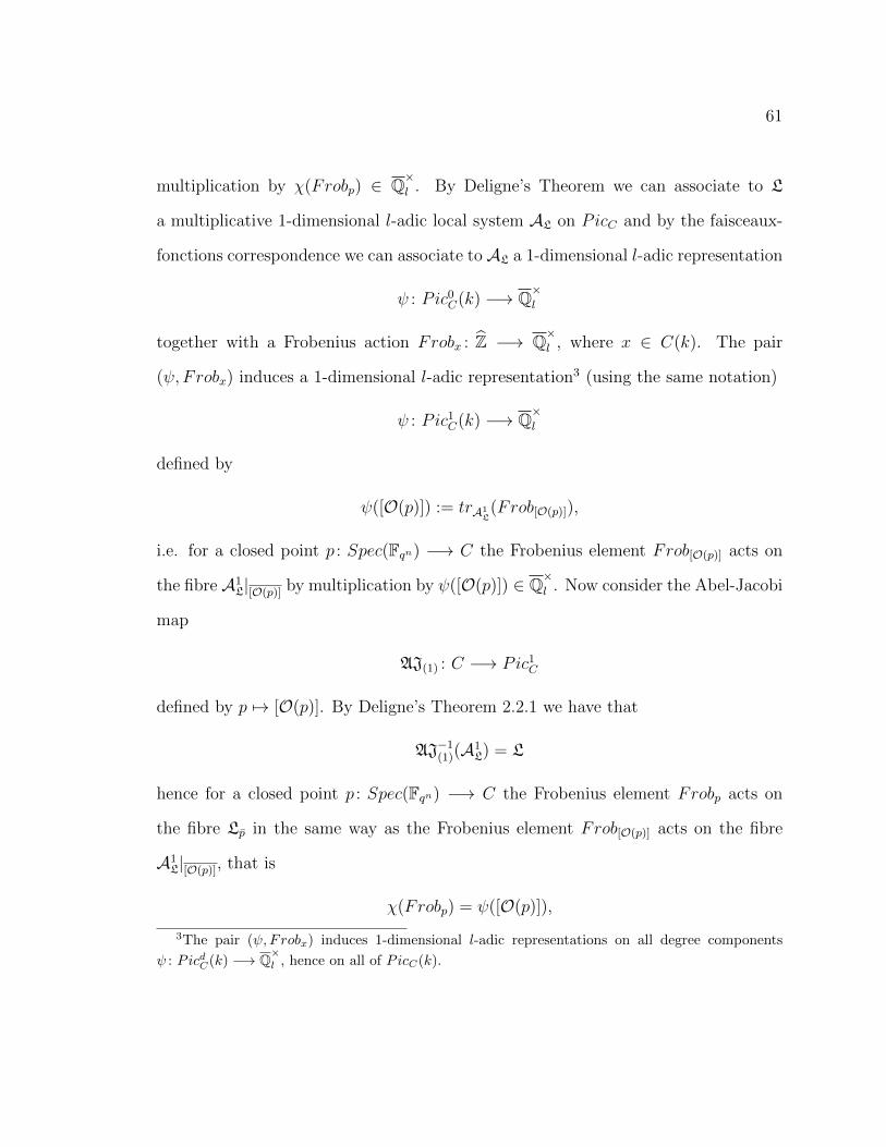
61

multiplication by χ(Frobp) ∈ Q×l . By Deligne’s Theorem we can associate to L

a multiplicative 1-dimensional l-adic local system AL on PicC and by the faisceaux-

fonctions correspondence we can associate to AL a 1-dimensional l-adic representation

ψ : Pic0C(k) −→ Q×l

together with a Frobenius action Frobx : Z −→ Q×l , where x ∈ C(k). The pair

(ψ, Frobx) induces a 1-dimensional l-adic representation3 (using the same notation)

ψ : Pic1C(k) −→ Q×l

defined by

ψ([O(p)]) := trA1L(Frob[O(p)]),

i.e. for a closed point p : Spec(Fqn) −→ C the Frobenius element Frob[O(p)] acts on

the fibre A1L|[O(p)] by multiplication by ψ([O(p)]) ∈ Q×l . Now consider the Abel-Jacobi

map

AJ(1) : C −→ Pic1C

defined by p 7→ [O(p)]. By Deligne’s Theorem 2.2.1 we have that

AJ−1(1)(A1

L) = L

hence for a closed point p : Spec(Fqn) −→ C the Frobenius element Frobp acts on

the fibre Lp in the same way as the Frobenius element Frob[O(p)] acts on the fibre

A1L|[O(p)], that is

χ(Frobp) = ψ([O(p)]),

3The pair (ψ, Frobx) induces 1-dimensional l-adic representations on all degree components

ψ : PicdC(k) −→ Q×l , hence on all of PicC(k).

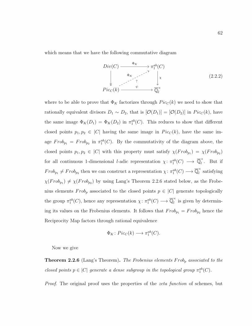
62

which means that we have the following commutative diagram

Div(C) πab1 (C)

PicC(k) Q×l

ΦK

ψ

χΦK

?

(2.2.2)

where to be able to prove that ΦK factorizes through PicC(k) we need to show that

rationally equivalent divisors D1 ∼ D2, that is [O(D1)] = [O(D2)] in PicC(k), have

the same image ΦK(D1) = ΦK(D2) in πab1 (C). This reduces to show that different

closed points p1, p2 ∈ |C| having the same image in PicC(k), have the same im-

age Frobp1 = Frobp2 in πab1 (C). By the commutativity of the diagram above, the

closed points p1, p2 ∈ |C| with this property must satisfy χ(Frobp1) = χ(Frobp2)

for all continuous 1-dimensional l-adic representation χ : πab1 (C) −→ Q×l . But if

Frobp1 6= Frobp2 then we can construct a representation χ : πab1 (C) −→ Q×l satisfying

χ(Frobp1) 6= χ(Frobp2) by using Lang’s Theorem 2.2.6 stated below, as the Frobe-

nius elements Frobp associated to the closed points p ∈ |C| generate topologically

the group πab1 (C), hence any representation χ : πab1 (C) −→ Q×l is given by determin-

ing its values on the Frobenius elements. It follows that Frobp1 = Frobp2 hence the

Reciprocity Map factors through rational equivalence

ΦK : PicC(k) −→ πab1 (C).

Now we give

Theorem 2.2.6 (Lang’s Theorem). The Frobenius elements Frobp associated to the

closed points p ∈ |C| generate a dense subgroup in the topological group πab1 (C).

Proof. The original proof uses the properties of the zeta function of schemes, but

63

here we will give a more geometric proof again using Deligne’s construction (diagram

1.1.2).

Assume that the image H := ΦK(Div(C)) ⊂ πab1 (C) of the Reciprocity Map is not

dense and denote by H its closure. Then there exists an open subset U containing

H. By Theorem 1.4.6 it corresponds to a finite, abelian, etale cover Y −→ C of some

degree d, which by Proposition 1.5.9 corresponds to a locally constant etale sheaf F

on C and to a d-dimensional representation

χ : πab1 (C) −→ GLd(Ql).

Here we can pass to a Ql-representation by making F into an l-adic local system. By

construction we have that for every closed point p ∈ |C| the action of the Frobenius

element Frobp on the fibre Fp is trivial, hence the representation χ|H : H −→ GLd(Ql)

is trivial. On the other hand taking the decomposition into irreducible, hence 1-

dimensional representations

χ = χ1 ⊕ χ2 ⊕ · · · ⊕ χd

each χi will correspond to a 1-dimensional l-adic representation

ψi : Pic0C(k) −→ Q×l

satisfying ψi = χi ΦK which are the trivial representations by construction. Hence

by diagram 4.2.3 we get that each χi and consequently the representation

χ : πab1 (C) −→ GLd(Ql)

is trivial. It follows that U = πab1 (C) and H = πab1 (C) completing the proof of Lang’s

Theorem.

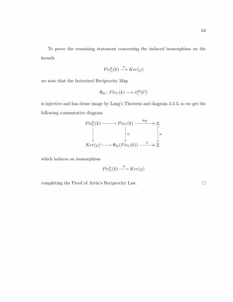
64

To prove the remaining statement concerning the induced isomorphism on the

kernels

Pic0C(k)

∼=−→ Ker(ϕ)

we note that the factorized Reciprocity Map

ΦK : PicC(k) −→ πab1 (C)

is injective and has dense image by Lang’s Theorem and diagram 4.2.3, so we get the

following commutative diagram

Pic0C(k) PicC(k) Z

Ker(ϕ) ΦK(PicC(k)) Z

deg

ϕ

∼= ∼=

which induces an isomorphism

Pic0C(k) Ker(ϕ)

∼=

completing the Proof of Artin’s Reciprocity Law.

Chapter 3

Tamely Ramified GeometricAbelian Class Field Theory

In this chapter we will present tamely ramified geometric abelian class field theory

which establishes a connection between the Picard group PicC,S of a smooth projective

curve over a finite field, where S is a finite set of points of the curve and the abelianized

tame etale fundamental group πt,ab1 (U) of the open complement.

We will begin with stating the main theorem of the tamely ramified theory in

different forms without going into the details and trace out a way how we will prove

it.

Then in the subsequent sections we will discuss and develop the background. In

particular we will define the basic concepts appearing in both sides of the correspon-

dence, namely the Picard group PicC,S and the tame etale fundamental group of

the open complement and we will also perform the necessary constructions leading

to a geometric proof of the main theorem, which finally will be provided in the last

chapter.

65

66

3.1 The Main Theorem

Let C be a smooth, projective, geometrically irreducible curve over a finite field

k = Fq, S = p1, p2, . . . , pn ⊂ |C| a finite set of closed points and U := C \ S the

open complement of S. Let K = k(C) be the function field and for every closed point

p ∈ |C| let Op be the completion of the local ring at the point p and Kp its quotient

field. For every p ∈ S we consider the kernel

Op1

:= Ker(Op×−→ (Op/mp)

×)

where we have Op/mp∼= Op/mp

1. Let IK :=∏′

p∈|C|K×p be the idele group of C,

IK,S := (∏

p/∈SK×p ×

∏p∈S Op

1)⋂IK be the subgroup of the ideles relative to S. Let

KS := K×⋂

IK,S ⊂ IK be the set of rational functions satisfying ordp(1− g) ≥ 1 for

all p ∈ S. We consider also the normal subgroup

∏p∈S Op

1×∏

p/∈S O×p ⊆ IK .

Furthermore let πab,t1 (U) be the abelianized tame etale fundamental group of the open

subscheme U ⊂ C. The main theorem of tamely ramified abelian class field theory is

the following:

Theorem 3.1.1 (Tamely Ramified Reciprocity Law, adelic form). The tamely ram-

ified Reciprocity Map

ΦK,S : IK,S/∏

p/∈S O×p πt,ab1 (U)

[(. . . , ap, . . . )p∈U ]∏

p∈U Frobordp(ap)p

ΦK,S

induces a map (also denoted by ΦK,S)

1cf. Theorem II.4.3 in [Neu07]

67

ΦK,S : K×\IK/∏

p∈S Op1×∏

p/∈S O×p −→ πt,ab1 (U)

fitting into the commutative diagram

Ker(deg) K×\IK/∏

p∈S Op1×∏

p/∈S O×p Z

Ker(ϕ) πt,ab1 (U) Z

deg

ϕ

ΦK,S can

such that there is an induced isomorphism on the kernels

Ker(deg)∼=−→ Ker(ϕ)

where ϕ : πt,ab1 (U) −→ Z is the map given by composing the natural map πt,ab1 (U) −→

πab1 (C) with the induced map πab1 (C) −→ Z (section 3.3).

In order to interpret this statement geometrically we need the following

Proposition 3.1.2. The inclusion IK,S → IK induces an isomorphism

KS\IK,S ∼= K×\IK

and hence an isomorphism

KS\IK,S/∏

p/∈S O×p ∼= K×\IK/∏

p∈S Op1×∏

p/∈S O×p .

Proof. The first statement is Proposition 4.6 (b) in [Mil08b], the second statement

then follows by dividing out with∏

p∈S Op1.

We can characterize this adelic double quotient in terms of geometric data asso-

ciated to the curve C in the following way

Proposition 3.1.3. There is an isomorphism

68

K×\IK/∏

p∈S Op1×∏

p/∈S O×p ∼= PicC,S(k)

between the adelic double coset space and isomorphism classes of invertible sheaves

on C together with fixed isomorphisms at each point p ∈ S

PicC,S(k) := ([G], ψpp∈S) | [G] ∈ PicC(k) and ψp : G ⊗OC Op/mp∼= Op/mp.

Proof. Given an invertible sheaf F on C with fixed isomorphisms at each p ∈ S

ψp : G ⊗OC Op/mp∼= Op/mp,

we choose a trivialization at the generic point ξ of C

fξ : F ⊗OC K∼=−→ K,

also a trivialization for every closed point p ∈ U

fp : F ⊗OC Op∼=−→ Op,

and at each p ∈ S a trivialization

fp∈S : F ⊗OC Op∼=−→ Op

such that fp∈S ≡ ψp mod mp. The natural morphism Op −→ K gives the diagram

for all p ∈ C

F ⊗OC Op ⊗Op K Op ⊗Op K

K K .

fp ⊗ idK

fξ

∼=

gp

∼=

The isomorphism gp is given by multiplication by an element ap ∈ K×. Moreover for

all but finitely many closed point p ∈ |C| we have that2 ap ∈ O×p , hence the invertible

sheaf F defines an element2cf. Lemma I.6.5 in [Har06]

69

(. . . , ap, . . . )p∈|C| ∈∏′

p∈|C|K×.

If we choose another trivialization at the generic point ξ

f′

ξ : F ⊗OC K∼=−→ K

then each element ap will be changed via left multiplication by an element in K×. If

we choose another trivializations at each p ∈ U

f′p : F ⊗OC Op

∼=−→ Op

then the element ap will be changed via right multiplication by an element in O×p .

Also if we choose another trivializations at each p ∈ S

f′p∈S : F ⊗OC Op

∼=−→ Op

satisfying fp∈S ≡ ψp mod mp then the element ap will be changed via right multipli-

cation by an element in Op1. Hence F defines an element in

K×\∏′

p∈|C|K×/

∏p∈S Op

1×∏

p/∈S O×p .

Now we use Claim 1.1.3 to get an element in

K×\IK/∏

p∈S Op1×∏

p/∈S O×p

which depends only on the isomorphism class of F by construction.

On the other hand given an element a = (. . . , ap, . . . ) ∈ IK we define a sheaf Fa

on C by

Fa(V ) := x ∈ K| a−1p x ∈ Op ∀ p ∈ V .

It follows from this local description that Fa defines a sheaf on C. Moreover changing

the coset representative a from the right by an element in∏

p∈S Op1×∏

p/∈S O×p does

not change anything in Fa and does not change ap mod mp at p ∈ S. Changing

70

from the left by an element b ∈ K× gives an isomorphism of sheaves Fab×−→ Fba, so

we have to prove that Fa is locally free of rank 1. If ap ∈ O×p for all p ∈ V then

Fa(V ) = OC(V ) by construction, hence it is free on V . Otherwise using Claim 1.1.3

we take an element t ∈ K× such that tap ∈ O×p . Now define V := p ∈ |C| : t ∈ O×p

and use the isomorphism Fat×−→ Fta which gives that Fa is locally free of rank 1 on V .

It remains to prove the existence of fixed isomorphisms at each point p ∈ S. For that

we use the approximation theorem3, which enables us to find an element aS ∈ K×

satisfying a−1S ap ≡ 1 mod mp for all p ∈ S. Hence we can modify the elements ap at

each p ∈ S such that the trivializations defined by ap

fp∈S : F ⊗OC Op∼=−→ Op

will give fixed isomorphisms

ψp : F ⊗OC Op/mp∼= Op/mp

well-defined modulo mp at each p ∈ S. These two constructions are inverses to each

other which completes the proof.

Now we can state the tamely ramified Reciprocity Law in a more geometric form:

Theorem 3.1.4 (Tamely Ramified Reciprocity Law, geometric form). The tamely

ramified Reciprocity Map

ΦK,S : Div(U) πt,ab1 (U)

p [Frobp]

induces a map

ΦK,S : PicC,S(k) −→ πt,ab1 (U)

3cf. Theorem II.3.4 in [Neu07].

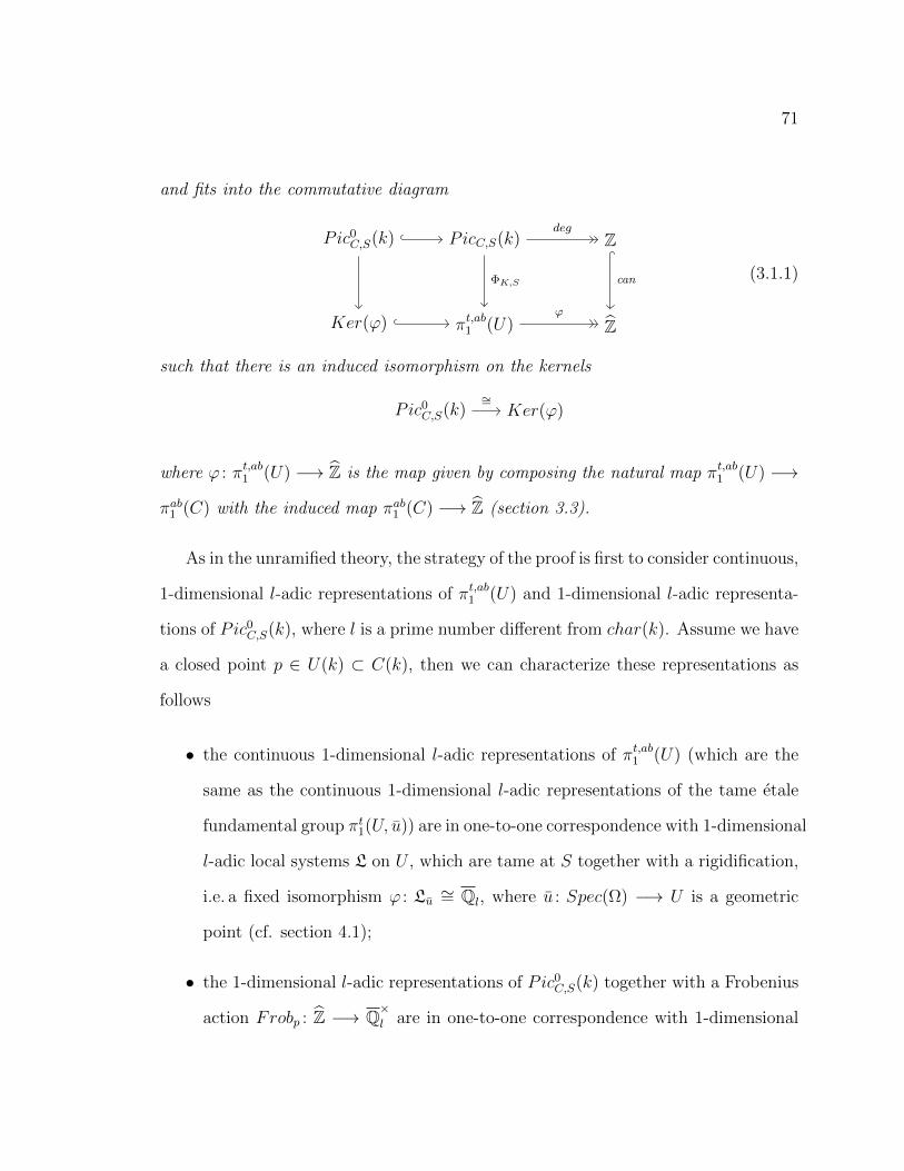
71

and fits into the commutative diagram

Pic0C,S(k) PicC,S(k) Z

Ker(ϕ) πt,ab1 (U) Z

deg

ϕ

ΦK,S can (3.1.1)

such that there is an induced isomorphism on the kernels

Pic0C,S(k) Ker(ϕ)

∼=

where ϕ : πt,ab1 (U) −→ Z is the map given by composing the natural map πt,ab1 (U) −→

πab1 (C) with the induced map πab1 (C) −→ Z (section 3.3).

As in the unramified theory, the strategy of the proof is first to consider continuous,

1-dimensional l-adic representations of πt,ab1 (U) and 1-dimensional l-adic representa-

tions of Pic0C,S(k), where l is a prime number different from char(k). Assume we have

a closed point p ∈ U(k) ⊂ C(k), then we can characterize these representations as

follows

• the continuous 1-dimensional l-adic representations of πt,ab1 (U) (which are the

same as the continuous 1-dimensional l-adic representations of the tame etale

fundamental group πt1(U, u)) are in one-to-one correspondence with 1-dimensional

l-adic local systems L on U , which are tame at S together with a rigidification,

i.e. a fixed isomorphism ϕ : Lu ∼= Ql, where u : Spec(Ω) −→ U is a geometric

point (cf. section 4.1);

• the 1-dimensional l-adic representations of Pic0C,S(k) together with a Frobenius

action Frobp : Z −→ Q×l are in one-to-one correspondence with 1-dimensional

72

l-adic local systems AL on PicC,S together with a rigidification, i.e. a fixed

isomorphism ψ : AL|0 ∼= Ql satisfying

m−1Ad+eL∼= AdL AeL

where

m : PicdC,S × PiceC,S −→ Picd+eC,S

is the group operation on PicC,S and 0: Spec(k) −→ PicC,S is the identity

section (cf. section 4.1).

Using these correspondences we will give a geometric construction adapting Deligne’s

argument in section 4.2, which gives a one-to-one correspondence between rigidified

1-dimensional l-adic local systems on U which are tame at S and rigidified multi-

plicative 1-dimensional l-adic local systems on PicC,S. Having done this we will get

the following diagram:

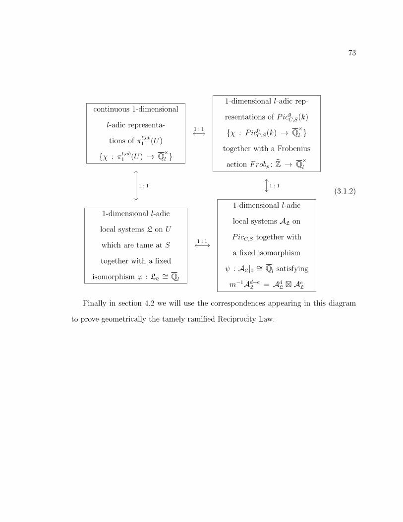
73

continuous 1-dimensional

l-adic representa-

tions of πt,ab1 (U)

χ : πt,ab1 (U) → Q×l

1-dimensional l-adic rep-

resentations of Pic0C,S(k)

χ : Pic0C,S(k) → Q×l

together with a Frobenius

action Frobp : Z → Q×l

1-dimensional l-adic

local systems L on U

which are tame at S

together with a fixed

isomorphism ϕ : Lu ∼= Ql

1-dimensional l-adic

local systems AL on

PicC,S together with

a fixed isomorphism

ψ : AL|0 ∼= Ql satisfying

m−1Ad+eL = AdL AeL

1 : 1

1 : 1

1 : 1

1 : 1(3.1.2)

Finally in section 4.2 we will use the correspondences appearing in this diagram

to prove geometrically the tamely ramified Reciprocity Law.

74

3.2 The Symmetric Power U (d) and the relative Pi-

card Scheme PicC,S

In this section we will define the symmetric powers U (d) and the Picard scheme PicC,S

functorially and establish the tamely ramified Abel-Jacobi map between them.

Let C be a smooth, projective curve over a field k, S = p1, p2, . . . , pn ⊂ |C| a

finite set of closed points, U := C \S the open complement of S and d ≥ 1 an integer.

Recall that in section 1.2 we defined the functor

DivdC : Sch/k −→ Set

which to a k-scheme T associates the set DivdC(T ) of relative effective Cartier divisors

of degree d on (C×Spec(k)T )/T ). By Proposition 1.2.6 this functor parametrizes pairs

(G, s), where G is an invertible sheaf on (C ×Spec(k) T )/T ) and s ∈ H0((C ×Spec(k)

T )/T ),G) \ 0 is a non-zero global section such that the subscheme defined by s is

flat over T .

Definition 3.2.1. We define an open subfunctor of DivdC

DivdU : Sch/k −→ Set

which to a k-scheme T associates the set DivdU(T ) of relative effective Cartier divisors

of degree d on (C ×Spec(k) T )/T such that if such a D ∈ DivdU(T ) is represented by a

class (G, s), then s|S×T 6= 0.

Now the proof of Theorem 1.2.10 can be applied word by word for our situation

and one can construct a canonical relative effective Cartier divisor Dcan on (C×Spec(k)

U (d))/U (d)), which implies the following

75

Theorem 3.2.2. Let C be a smooth, projective curve over a field k, S = p1, p2, . . . , pn ⊂

|C| a finite set of closed points, U := C \ S the open complement of S and d ≥ 1

an integer. Then for any relative effective Cartier divisor D on (C ×Spec(k) T )/T ,

that is represented by a class (G, s), where s|S×T 6= 0 there exists a unique morphism

α : T −→ C(d) factorizing through α : T −→ U (d) such that

D = (idC × α)−1(Dcan),

that is the functor DivdU is representable by U (d).

Now let us turn to the Picard scheme PicC,S.

Definition 3.2.3. For an integer d ∈ Z we define the Picard functor of degree d with

respect to S as the functor from the category of schemes over k to the category of

abelian groups

PicdC,S : Sch/k −→ Ab

which to a k-scheme T associates the abelian group

PicdC,S(T ) := (G, ψpp∈S)/pr−12 (Picd(T ))

where G ∈ Pic(C ×Spec(k) T ) such that deg(Gt) = d for all t ∈ T together with fixed

isomorphisms ψp : G ⊗Op×T Op×T/mp×T∼=−→ Op×T/mp×T at each p ∈ S.

We note that for a point p ∈ S we have an isomorphism of functors

PicdC∼=−→ PicdC,p

given by sending G ∈ PicdC(T ) to G⊗pr−12 (G|p×T ), which has a canonical trivialization

along p × T , where pr2 : C ×Spec(k) T −→ T is the second projection. On the other

way round we use the forgetful functor sending G, ψpp∈S to G. So the fibres of

the natural (forgetful) transformation

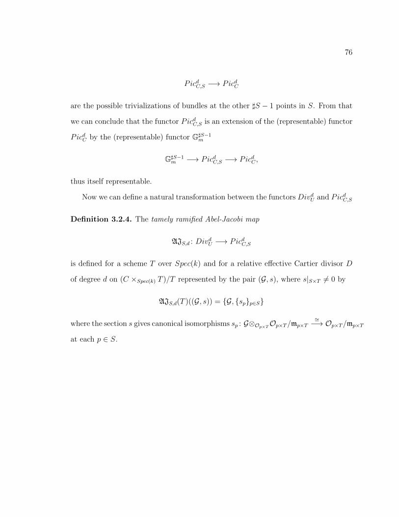
76

PicdC,S −→ PicdC

are the possible trivializations of bundles at the other ]S − 1 points in S. From that

we can conclude that the functor PicdC,S is an extension of the (representable) functor

PicdC by the (representable) functor G]S−1m

G]S−1m −→ PicdC,S −→ PicdC ,

thus itself representable.

Now we can define a natural transformation between the functors DivdU and PicdC,S

Definition 3.2.4. The tamely ramified Abel-Jacobi map

AJS,d : DivdU −→ PicdC,S

is defined for a scheme T over Spec(k) and for a relative effective Cartier divisor D

of degree d on (C ×Spec(k) T )/T represented by the pair (G, s), where s|S×T 6= 0 by

AJS,d(T )((G, s)) = G, spp∈S

where the section s gives canonical isomorphisms sp : G⊗Op×TOp×T/mp×T∼=−→ Op×T/mp×T

at each p ∈ S.

77

3.3 The Tame Fundamental Group

In this section we will define the tame fundamental group of a regular integral scheme

that is separated of finite type over a (finite) field and present some of its most

important properties according to the scope of our purposes. The main references for

this section are [GM71], 5.7.15-16 in [Sza09b], A.I. in [FK88] and II.7. in [Neu07].

Let K be a field together with a discrete valuation v, denote Ov, k(v) and v(K×)

the valuation ring, the residue field and the value group of v respectively. Let L/K

be a finite separable field extension, then by II.8.1 in [Neu07] there exist only finitely

many non-equivalent extensions w/v of the discrete valuation v to the field L and

these are also discrete valuations.

Definition 3.3.1. A finite separable field extension L/K is said to be tamely ramified

with respect to the valuation v of K if for each extension w of v to L we have

1. char(k(v)) - e where e := [w(L×) : v(K×)] is the ramification index of w/v and

2. the residue field extension k(w)/k(v) is separable.

Tamely ramified extensions have the following properties4

Proposition 3.3.2. 1. For a tower of field extensions M ⊃ L ⊃ K the extension

M/K is tamely ramified if and only if L/K and M/L are tamely ramified with

respect to any extension z/w/v;

2. if L/K and M/K are tamely ramified with respect to v, then the compositum

LM/K is also tamely ramified with respect to v;

4We assume that every field extension L,M,K′/K and their composita are contained in a fixed

algebraic closure K/K.

78

3. let L/K be tamely ramified with respect to v and K′/K be an arbitrary field

extension together with a discrete valuation v′

extending v, then the extension

LK′/K

′is tamely ramified with respect to v

′;

4. let L/K be tamely ramified with respect to v and let M/K be the smallest Galois

extension of K containing L, then M/K is also tamely ramified with respect to

v;

5. if L/K is tamely ramified with respect to v, then L ⊗K Kv/Kv is also tamely

ramified, meaning that each summand Lw is tamely ramified over Kv (see The-

orem II.8.3 in [Neu07]).

Proof. cf. Lemma 2.1.3. and Corollaire 2.1.4. in [GM71].

Now we define the notion tamely ramified for schemes:

Definition 3.3.3. Let X be a normal, integral scheme, U ⊂ X an open subscheme,

such that the closed subset S = X \ U is of at least codimension 1. Then a finite

morphism f : Y −→ X is said to be tamely ramified with respect to S if

1. f |f−1U is a finite etale cover f−1U ⊆ Y −→ U and

2. Y is tamely ramified over Spec(OX,s) for each codimension 1 point s ∈ S, that

is the fibre Ys := Y ×X Spec(OX,s) is a finite direct product Ys =∏n

i=1 Spec(Li)

of spectra of finite separable field extensions of the quotient field K of OX,s, as

the generic point of Spec(OX,s) is contained in U , and each extension Li/K is

tamely ramified with respect to the valuation given by OX,s.

Tamely ramified coverings have the following properties:

79

Proposition 3.3.4. Let f : Y −→ X be a morphism of schemes and g : X′ −→ X

a surjective, etale base change morphism. Then Y is tamely ramified over X with

respect to S if and only if Y ×X X′

is tamely ramified over X′

with respect to g−1(S).

Proposition 3.3.5. 1. Let Y/X and Z/X be schemes over X, f : Y −→ Z and

g : Z −→ X be finite morphisms g being surjective. Then Y is tamely ramified

over X with respect to S if and only if Z is tamely ramified over X with respect

to S and Y is tamely ramified over Z with respect to g−1(S).

2. Let f : Y −→ X be a tamely ramified cover with respect to S, where S is a

divisor with normal crossings. Let g : X′ −→ X be a morphism, where X

′is

a normal scheme such that S′

:= g−1(S) is defined and is again a divisor with

normal crossings. Then f′: X

′ ×X Y −→ X′

is a tamely ramified cover with

respect to S′.

Proof. cf. Lemma 2.2.5, Lemma 2.2.7 and Lemma 2.3.6 in [GM71].

Assume now that X is a connected regular integral scheme that is separated of

finite type over a (finite) field k and S ⊂ X is a divisor with normal crossings5. Let

U := X \ S be the open complement.

Let Fett,S/X be the category of tamely ramified coverings of X with respect to S.

Let u : Spec(Ω) −→ U be a fixed geometric point and define the tame fibre functor

at the geometric point u

F t,Su : Fett,S/X −→ Set

5In particular the case we are most interested in when X is a smooth projective geometricallyirreducible curve over a finite field and S ⊂ X is a finite set of closed points.

80

which to a tamely ramified cover f : Y −→ X with respect to S associates the

underlying set of the fibre over u, i.e. F t,Su (Y, f) := the underlying set of Yu :=

Y ×X Spec(Ω) and for a morphism

Y Z

X

g

tame w.r.t. Stame w.r.t. S

it associates the set-theoretic map F t,Su (Y ) −→ F t,S

u (Z) induced by the morphism of

geometric fibres Y ×X Spec(Ω) −→ Z ×X Spec(Ω).

Definition 3.3.6. Let X,S, U and u be as above. Then the tame etale fundamental

group πt1(X,S, u) of X with respect to S at u is defined as the automorphism group

of the tame fibre functor F t,Su on Fett,S/X. If there is no confusion we will denote

this group as πt1(U, u) and call it the tame etale fundamental group of U at u.

Theorem 3.3.7. Let X be a connected regular integral scheme that is separated and

of finite type over a (finite) field, S ⊂ X a divisor with normal crossings, U := X \S

its open complement and u a geometric point of U ⊂ X. Then

• the group πt1(U, u) is profinite and its action on F t,Su (Y ) is continuous for every

Y in Fett,S/X.

• The fibre functor F t,Su induces an equivalence of the category Fett,S/X with the

category of finite continuous left πt1(U, u)-sets. Connected covers corresponds to

sets with transitive action, and Galois covers to finite quotients of πt1(U, u).

Proof. cf. Corollaire 2.4.4. in [GM71].

81

Example 3.3.8. Let X = Pnks , S = Pn−1ks and U = An

ks , where ks is a separable closed

field. Then πt1(Anks , u) = 1 is trivial. To prove this we use an induction argument.

For n = 1 it is enough to show that any finite map f : Y −→ P1ks , that is etale

over A1ks ⊂ P1

ks and tamely ramified at infinity, is an isomorphism. Let ω be the

differential dt on P1ks . It has a double pole at infinity and no other poles or zeroes.

By the Hurwitz-Riemann formula we have that 2g(Y )− 2 = n(−2) + r∞ − 1, where

n is the degree of the map f and r∞ is the ramification index at infinity. Now we

have the inequality −2n + n − 1 ≥ 2g(Y ) − 2, from which it follows that n = 1.

Now assume that f : Y −→ Pn+1ks is a finite map, that is etale over An+1

ks ⊂ Pn+1ks

and tamely ramified along Pnks . But then the restriction of f to any n-dimensional

affine subspace will be tame along any n − 1-dimensional projective subspace of the

complement, hence trivial by the induction hypothesis. So it implies that f must be

an isomorphism, completing the proof.

Let Fet/U , Fet/X and Fin/X be the categories of finite etale covers of U , finite

etale covers of X and finite covers of X respectively. Then we have the following

inclusions of categories as full subcategories

Fet/X ⊆ Fett,S/X ⊆ Fin/X

and also

Fett,S/X ⊆ Fet/U

which induce the following surjective maps

πt1(U, u) −→ π1(X, u) −→ 1

and

82

π1(U, u) −→ πt1(U, u) −→ 1 .

The tame etale fundamental group has the usual properties of the algebraic fun-

damental group:

Proposition 3.3.9. 1. Changing the base point u to u′

the tame fundamental

groups become isomorphic πt1(U, u)∼=−→ πt1(U, u

′) determined up to an inner

automorphism.

2. Let g : X′ −→ X be a morphism, where X

′is a normal scheme such that S

′:=

g−1(S) is defined and is again a divisor with normal crossings and u′

a geometric

point of U′ ⊂ X

′, where U

′:= X

′ \ S ′ is the open complement. Then there is

an induced group homomorphism πt1(U′, u′) −→ πt1(U, u) determined up to an

inner automorphism of πt1(U, u).

Proof. cf. 2.4.5 in [GM71].

Chapter 4

The Proof of the Main Theorem ofthe Tamely Ramified Theory

In this chapter we begin with final preliminary works proving the correspondences

appearing in diagram 3.1.2 and after that we give a geometric proof of the Main

Theorem 3.1.4 adapting Deligne’s geometric argument.

4.1 Preliminary Constructions

Let C be a smooth, projective, geometrically irreducible curve of genus g over a finite

field k = Fq, S = p1, p2, . . . , pn ⊂ |C| a finite set of closed points and U := C \ S

the open complement of S.

Let us begin to prove the correspondence between representations of πt,ab1 (U) and

local systems on U which are tame at S. First we define 1-dimensional l-adic local

systems on U which are tame at S.

Definition 4.1.1. Let L be a 1-dimensional l-adic local system on U ⊂ C defined by

a continuous 1-dimensional l-adic representation χ : π1(U, u) −→ Q×l . Then L is said

to be tame at S = X \ U if for every s ∈ S the induced map

83

84

π1(Spec(Ks), s) −→ π1(U, u)χ−→ Q×l

where Ks is the stalk at the generic point of Spec(OX,s), induces a factorization

π1(Spec(Ks), s) π1(U, u) Q×l

πt1(Spec(Ks), s) .

χ

∃

In other words the induced representation π1(Spec(Ks), s) −→ Q×l is trivial on the

inertia subgroup Is ⊂ π1(Spec(Ks), s), where the inertia subgroup is defined as the

kernel of the natural surjective map π1(Spec(Ks), s) πt1(Spec(Ks), s).

Now we can state

Theorem 4.1.2. There is a one-to-one correspondence between

continuous 1-dimensional

l-adic representa-

tions of πt,ab1 (U)

χ : πt,ab1 (U) → Q×l

1-dimensional l-adic

local systems L on U

which are tame at S

together with a fixed

isomorphism ϕ : Lu ∼= Ql

1 : 1

Proof. We consider the following diagram of categories and the natural functors be-

tween them

Fet/U Fet/Spec(Ks)

Fett,S/X Fett/Spec(Ks)

restriction

restriction

which is a push out diagram, hence it induces a push out diagram

85

π1(U, u) π1(Spec(Ks), s)

πt1(U, u) πt1(Spec(Ks), s) .

Now given a continuous 1-dimensional l-adic representation χ : πt1(U, u) −→ Q×l , it

induces a continuous 1-dimensional l-adic representation χ : π1(U, u) −→ Q×l such

that the restriction map

π1(Spec(Ks), s) −→ π1(U, u)χ−→ Q×l

induces a factorization at each s ∈ S

π1(Spec(Ks), s) π1(U, u) Q×l

πt1(Spec(Ks), s)

χ

∃

that is we have a rigidified 1-dimensional l-adic local system L on U which is tame

at S by section 1.5 and by the definition of tameness of a local system.

On the other hand if we are given a rigidified 1-dimensional l-adic local system L

on U which is tame at S, it induces a continuous 1-dimensional l-adic representation

χ : π1(U, u) −→ Q×l together with the above factorization, hence the above push out

diagram induces a continuous 1-dimensional l-adic representation χ : πt1(U, u) −→ Q×l .

These constructions are inverses to each other. Now we can pass to the abelianized

fundamental groups, as 1-dimensional representations naturally factor through them

completing the proof of the Theorem.

Next we want to analyze the tamely ramified Abel-Jacobi map (cf. section 3.2)

and determine the fibres.

86

Given an integer d ≥ 1 and a geometric point ([G], ψpp∈S) ∈ PicdC,S we have the

following condition concerning the surjectivity of the tamely ramified Abel-Jacobi

map

Condition 4.1.3. The fibre AJ−1S,d([G], ψpp∈S) 6= ∅ is not empty if there exists a

non-zero global section s ∈ H0(C,G) \ 0 generating the fibre G ⊗OC Op at each

p ∈ S such that the induced map sp : G ⊗OC Op/mp −→ Op/mp coincides with the

fixed trivialization ψp : G ⊗OC Op/mp −→ Op/mp for all p ∈ S.

Now consider the exact sequence of sheaves on C

0 −→ O(−S) −→ OC −→ OS −→ 0

where OC is the structure sheaf of C, O(−S) is the ideal sheaf of the closed subscheme

S ⊂ C and OS is the structure sheaf of S. As G is locally free, tensoring with G we

get the exact sequence

0 −→ G(−S) −→ G −→ G/G(−S) −→ 0

where G/G(−S) =⊕

p∈S(G ⊗OC Op/mp). This exact sequence induces a long exact

sequence in cohomology

0 H0(C,G(−S)) H0(C,G) H0(C,G/G(−S))

H1(C,G(−S)) . . .

ev

δ

Then Condition 4.1.3 is equivalent to

87

ψpp∈S ∈ Ker(δ)

In particular this is the case if the evaluation map in cohomology is surjective

H0(C,G)ev−→ H0(C,G/G(−S)) −→ 0.

From the long exact sequence it follows that this is the case if

H1(C,G(−S)) = 0.

By Serre duality

H1(C,G(−S)) ∼= H0(ωC ⊗ G(−S)−1)∨,

hence H1(C,G(−S)) vanishes if deg(G(−S)) ≥ 2g − 1. From the exact sequence we

started with it follows that

deg(G(−S)) = d− ]S

where d = deg(G). Putting everything together we get

Proposition 4.1.4. The tamely ramified Abel-Jacobi map AJS,d is surjective if d ≥

2g − 1 + ]S.

Now we can determine the fibres of the map AJS,d for d ≥ 2g − 1 + ]S.

Proposition 4.1.5. Given a geometric point (G, ψpp∈S) ∈ PicdC,S and an integer d

satisfying d ≥ 2g − 1 + ]S, we have the exact sequence

0 −→ H0(C,G(−S)) −→ H0(C,G)ev−→ H0(C,G/G(−S))

δ−→ 0

and for the fibre we have the isomorphism

χ : ev−1(ψpp∈S)∼=−→ AJ−1

S,d((G, ψpp∈S))

88

given by

s 7→ div(s)

for an s ∈ ev−1(ψpp∈S) ⊂ H0(C,G).

Proof. Injectivity : given sections s, s′ ∈ ev−1(ψpp∈S) with div(s) = div(s

′), then by

definition we have that

s− s′ ∈ Ker(ev) ∼= H0(C,G(−S))

so s′= s− t for some t ∈ H0(C,G(−S)). But we also have that

t ∈ H0(C,G ⊗ O(−div(s)))

because of the equality div(s) = div(s′). Now the degree

deg(G ⊗O(−div(s))) = 0

is zero, hence H0(C,G ⊗ O(−div(s))) = k, that is t must be a constant. But as

t ∈ H0(C,G(−S)) as well, which means that t vanishes at the points p ∈ S, it follows

that t = 0 ∈ k, hence s = s′.

Surjectivity : Given an effective divisorD ∈ AJ−1S,d((G, ψpp∈S)), it defines a canon-

ical section sD : OC → O(D) satisfying 0 6= sD|p = ψp for all p ∈ S and O(D) ∼= G.

This means that sD ∈ ev−1(ψpp∈S) ⊂ H0(C,G) and div(s) = D, which completes

the proof of the Proposition.

The main result that we will need in the next section is

Theorem 4.1.6. If the degree satisfies d ≥ 2g − 1 + ]S then the tamely ramified

Abel-Jacobi map AJS,d : U (d) −→ PicC,S is a surjective morphism. For a geometric

point ([G], ψpp∈S) ∈ PicdC,S the fibre is isomorphic to the affine subspace

89

AJ−1S,d((G, ψpp∈S)) ∼= ev−1(ψpp∈S) ⊂ H0(C,G)

which is an H0(C,G(−S))-torsor.

90

4.2 A Geometric Proof

In this section we turn to the proof of the Main Theorem 3.1.4 using a geometric

argument adapting Deligne’s proof of the unramified theory.

First we want to prove the tame version of Deligne’s Theorem which gives the

connection between rigidified 1-dimensional l-adic local systems on U which are tame

at S and rigidified multiplicative 1-dimensional l-adic local systems on the Picard

scheme PicC,S appearing in the bottom row of diagram 3.1.2.

Theorem 4.2.1. There is a one-to-one correspondence between

1-dimensional l-adic

local systems L on U

which are tame at S

together with a fixed

isomorphism ϕ : Lu ∼= Ql

1-dimensional l-adic

local systems AL on

PicC,S together with

a fixed isomorphism

ψ : AL|0 ∼= Ql satisfying

m−1Ad+eL = AdL AeL

1 : 1

Proof. Given a 1-dimensional l-adic local system L on U which is tame at S we can

construct a 1-dimensional l-adic local system L(d) on U (d) in the same way as we did

in section 2.1 by defining

L(d) := ((Symd|Ud)∗Ld)Sd

where Symd : Cd −→ C(d) is the symmetrization morphism. Moreover this 1-dimensional

l-adic local system L(d) will be tame at the codimension 1 part of the complement

C(d) \ U (d) ⊃ Z :=⋃s∈S s × U (d−1) by the following argument. Let η be the generic

point of s×U (d−1) and η a generic point of s×Ud mapping to η under the symmetriza-

tion morphism. Assume that the 1-dimensional l-adic local system L(d) on U (d) is

91

defined by the continuous 1-dimensional l-adic representation χ : π1(U (d), u) −→ Q×l .

Then we have to prove that the induced representation χ : π1(Kη, η) −→ Q×l fac-

tors through πt1(Kη, η). The morphism Symd is etale over the open subscheme

C(d) \ ∆ ⊂ C(d), where ∆ is the big diagonal, that is where some of the points

coincide, which means that Symd is etale over the generic point η. By Proposition

3.3.4 we know that tame etale coverings of U (d) form a full subcategory of the tame

etale coverings of Ud, hence there is a surjective morphism between the inertia groups

Iη Iη. Now assume that Ld is tame at η. Then we claim that L(d) is tame at η.

To prove this we recall that (Symd)−1L(d)∼=−→ Ld, so tameness of Ld at η means

that we have the commutative diagram

Iη Iη

π1(Kη, η) π1(Kη, η) Q×l

πt1(Kη, η) πt1(Kη, η) .

χ

As by assumption the representation π1(Kη, η) −→ Q×l becomes trivial on the inertia

subgroup Iη and the map between the inertia subgroups Iη Iη is surjective, it

follows that the representation π1(Kη, η) −→ Q×l also becomes trivial on the inertia

subgroup Iη, hence L(d) is tame at η, as wanted.

It remains to prove that Ld is tame along⋃s∈S s × Ud−1. As this is a product,

we have to prove that Ld−1 is tame along⋃s∈S s× Ud−2. It finally reduces to show

that L is tame along S ⊂ C, which is our starting assumption, completing the proof

of the claim, that L(d) is tame along Z :=⋃s∈S s× U (d−1).

92

Now consider the universal family of invertible sheaves Guniv on

C ×Spec(k) PicdC,S

π−→ PicdC,S.

By definition for each closed point y := [G, ψpp∈S] ∈ PicdC,S the restrictions Guniv,y of

the universal invertible sheaf to the fibres Cy have degree d and if the degree satisfies

d ≥ 2g − 1 + ]S then we have fibrewise exact sequences

0→ H0(Cy,Guniv,y(−S))→ H0(Cy,Guniv,y)→ H0(Cy,Guniv,y/Guniv,y(−S))→ 0.

Now we need the following theorem

Theorem 4.2.2 (Grauert, Grothendieck). Let f : X −→ Y be a projective morphism

of noetherian schemes with Y integral and F a coherent sheaf on X, flat over Y .

Suppose that for some i the function

hi(y,F) := dimk(y)Hi(Xy,Fy)

is constant on Y . Then Rif∗(F) is locally free on Y and for every y the natural map

Rif∗(F)⊗ k(y) −→ H i(Xy,Fy)

is an isomorphism.

Proof. cf. II.12.9 Corollary in [Har06].

By this theorem we get an exact sequence of locally free sheaves on PicdC,S

0 −→ π∗Guniv(−S) −→ π∗Gunivev−→ π∗Guniv/Guniv(−S) −→ 0. (4.2.1)

As the restrictions Guniv,y have trivializations ψuniv,p : Guniv,y⊗OCyOCy/mp,y

∼=−→ OCy/mp,y

at each point p ∈ S, the sheaf π∗Guniv/Guniv(−S) has a canonical global section suniv

given by these trivializations. Now we claim that U (d) is isomorphic to the closed

subscheme ev−1suniv ⊂ π∗Guniv fitting into the commutative diagram

93

ev−1suniv ⊂ π∗Guniv π∗Guniv/Guniv(−S)

U (d) PicdC,S .

ev

AJS,d

∼=

suniv

To prove this we consider a closed point y := [G, ψpp∈S] ∈ PicdC,S. For the fibre

AJ−1S,d(y) we have the isomorphism AJ−1

S,d(y) ∼= ev−1ψpp∈S. The image of y under the

universal section is just suniv(y) = ψpp∈S, thus we get the isomorphism AJ−1S,d(y) ∼=

ev−1suniv(y). This gives a morphism U (d) −→ ev−1suniv. To construct the inverse map

we note that π∗Guniv parametrizes tuples (G, s, ψpp∈S), where G is an invertible sheaf

on C, s ∈ H0(C,G) \ 0 is a non-zero global section which does not vanish at the

points p ∈ S and ψpp∈S are fixed isomorphisms ψp : G ⊗OC Op/mp∼= Op/mp. It

follows from this description that ev−1suniv parametrizes tuples (G, s, ψpp∈S) where

ψp(sp) = 1 ∈ Op/mp at each p ∈ S and we can define a morphism ev−1suniv −→ U (d)

by sending

(G, s, ψpp∈S, ψp(sp) = 1) 7→ div(s),

that is inverse to the morphism U (d) −→ ev−1suniv. Moreover ev−1suniv ⊂ π∗Guniv is

a closed subscheme being the inverse image of the closed subscheme sunivPicdC,S ⊂

π∗Guniv/Guniv(−S), proving the claim.

Next we take a projective closure of U (d) defined by the following diagram

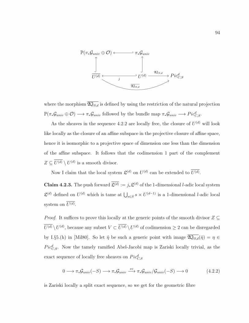
94

P(π∗Guniv ⊕O) π∗Guniv

U (d) U (d) PicdC,Sj

AJS,d

AJS,d

where the morphism AJS,d is defined by using the restriction of the natural projection

P(π∗Guniv ⊕O) −→ π∗Guniv followed by the bundle map π∗Guniv −→ PicdC,S.

As the sheaves in the sequence 4.2.2 are locally free, the closure of U (d) will look

like locally as the closure of an affine subspace in the projective closure of affine space,

hence it is isomorphic to a projective space of dimension one less than the dimension

of the affine subspace. It follows that the codimension 1 part of the complement

Z ⊆ U (d) \ U (d) is a smooth divisor.

Now I claim that the local system L(d) on U (d) can be extended to U (d).

Claim 4.2.3. The push forward L(d) := j∗L(d) of the 1-dimensional l-adic local system

L(d) defined on U (d) which is tame at⋃s∈S s × U (d−1) is a 1-dimensional l-adic local

system on U (d).

Proof. It suffices to prove this locally at the generic points of the smooth divisor Z ⊆

U (d) \U (d), because any subset V ⊂ U (d) \U (d) of codimension ≥ 2 can be disregarded

by I.§5.(h) in [Mil80]. So let η be such a generic point with image AJS,d(η) = η ∈

PicdC,S. Now the tamely ramified Abel-Jacobi map is Zariski locally trivial, as the

exact sequence of locally free sheaves on PicdC,S

0 −→ π∗Guniv(−S) −→ π∗Gunivev−→ π∗Guniv/Guniv(−S) −→ 0 (4.2.2)

is Zariski locally a split exact sequence, so we get for the geometric fibre

95

AJ−1S,d(η) ∼= η × An

ks

where n = d− g + 1− ]S. Now assume that L(d) is tame on U (d) along the divisor in

the compactification U (d). Then the restriction

L(d)|η×Anks

is defined by a continuous 1-dimensional l-adic representation

χ : πt,ab1 (Anks) −→ Q×l

which must be trivial, as πt,ab1 (Anks) = 1 is trivial by Example 3.3.8. It then follows

that L(d) extends naturally to

η × Anks = η × Pn−1

ks

and hence defines a 1-dimensional l-adic local system L(d) on U (d), which is uniquely

defined by the construction.

So it remains to prove that L(d) is tame on U (d) along the divisor in the compact-

ification U (d). For that we recall that the closed subscheme U (d) ⊂ π∗Guniv can be

described as isomorphism classes of tuples (G, s, ψpp∈S) where ψp(sp) = 1 ∈ Op/mp

at each p ∈ S. So the projective closure U (d) ⊂ P(π∗Guniv ⊕ O) is given as the

isomorphism classes of (G, [s : t], ψpp∈S) where ψp(s) = t for all p ∈ S and

(s, t) ∈ H0(C,G) ⊕ k (as Ud is given by setting t = 1). The section s can not

be 0 at any point in U (d), because the condition ψp(s) = t would imply t = 0, which

can not be the case. Thus we can define a map

α : U (d) −→ C(d)

by sending (G, [s : t], ψpp∈S, (ψp(s) = t)p∈S) 7→ (G, s)). We can describe the bound-

ary as follows

96

∂U (d) := U (d) \ U (d) = (G, [s : t], ψpp∈S) | t = 0, sp = 0 = PH0(C,G(−S)).

Thus the image of the boundary is α(∂U (d)) = S ×C(d−]S) ⊂ C(d). Now consider the

following fibre product diagram

Cd ×C(d) U (d) Cd

U (d) C(d) .

q

p Sym

α

Since the local system Ld is tame on Cd along⋃s∈S s×Cd−1, by Proposition 3.3.4 the

pull-back q−1Ld will be tame on Cd×C(d)U (d) along the pull-back q−1(⋃s∈S s×Cd−1).

Now as before at the generic point η of α(∂U (d)) the symmetrization morphism Sym

is etale, thus the projection p is etale over a generic point η of ∂U (d), hence using the

descent argument as before we can conclude that L(d) is tame on U (d) along ∂U (d),

completing the proof of the claim.

Now we can apply the relative homotopy exact sequence theorem (1.4.13) to the

compactified tamely ramified Abel-Jacobi map AJS,d : U (d) −→ PicdC,S taking into

account Theorem 4.1.6 to get the exact sequence

π1(Pd−g−]Sks , u) π1(U (d), u) π1(PicdC,S, u) 1

where ks is the separable closure of the base field k. We know from Example 1.4.12

that π1(Pd−g−]Sks , u) = 1 is trivial, hence we get an isomorphism

π1(U (d), u) ∼= π1(PicdC,S, u)

which induces an isomorphism between the abelianized etale fundamental groups

πab1 (U (d)) ∼= πab1 (PicdC,S).

97

This means that to the continuous 1-dimensional l-adic representation

χL(d) : πab1 (U (d)) −→ Q×l

corresponds a unique continuous 1-dimensional l-adic representation

χAdL : πab1 (PicdC,S) −→ Q×l

which again corresponds (section 1.5) to a unique 1-dimensional l-adic local system

AdL on PicdC,S together with a fixed isomorphism ψ : AdL|d0∼= Ql. To prove further

that AdL extends to PicC,S and satisfies the multiplicative property we refer to the

proof of Deligne’s Theorem 2.2.1.

On the other way round let a rigidified multiplicative 1-dimensional l-adic local

system AL on PicC,S be given. Then we consider the tamely ramified Abel-Jacobi

map

AJS,1 : U −→ Pic1C,S

and by Proposition 1.5.12 the pull-back

L := AJ−1S,1A1

L

is a 1-dimensional l-adic local system on U together with a rigidification. We have to

prove that L is tame along S ⊂ C. For that we note that A0L on Pic0

C,S is defined by

a 1-dimensional l-adic representation χ : Pic0C,S(k) −→ Q×l by Theorem 4.2.4. Now

consider the multiplication by q − 1 map

[q − 1] : Pic0C,S(k) −→ Pic0

C,S(k)

fitting into the diagram

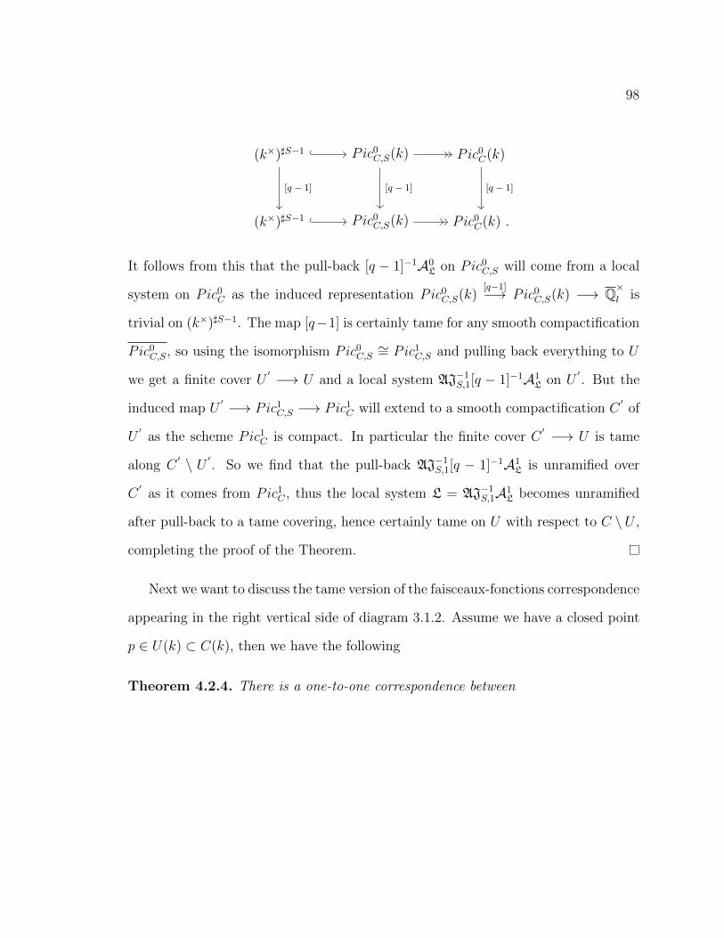
98

(k×)]S−1 Pic0C,S(k) Pic0

C(k)

(k×)]S−1 Pic0C,S(k) Pic0

C(k) .

[q − 1] [q − 1] [q − 1]

It follows from this that the pull-back [q − 1]−1A0L on Pic0

C,S will come from a local

system on Pic0C as the induced representation Pic0

C,S(k)[q−1]−→ Pic0

C,S(k) −→ Q×l is

trivial on (k×)]S−1. The map [q−1] is certainly tame for any smooth compactification

Pic0C,S, so using the isomorphism Pic0

C,S∼= Pic1

C,S and pulling back everything to U

we get a finite cover U′ −→ U and a local system AJ−1

S,1[q − 1]−1A1L on U

′. But the

induced map U′ −→ Pic1

C,S −→ Pic1C will extend to a smooth compactification C

′of

U′

as the scheme Pic1C is compact. In particular the finite cover C

′ −→ U is tame

along C′ \ U ′ . So we find that the pull-back AJ−1

S,1[q − 1]−1A1L is unramified over

C′

as it comes from Pic1C , thus the local system L = AJ−1

S,1A1L becomes unramified

after pull-back to a tame covering, hence certainly tame on U with respect to C \U ,

completing the proof of the Theorem.

Next we want to discuss the tame version of the faisceaux-fonctions correspondence

appearing in the right vertical side of diagram 3.1.2. Assume we have a closed point

p ∈ U(k) ⊂ C(k), then we have the following

Theorem 4.2.4. There is a one-to-one correspondence between

99

1-dimensional l-adic rep-

resentations of Pic0C,S(k)

χ : Pic0C,S(k) → Q×l

together with a Frobenius

action Frobp : Z → Q×l

1-dimensional l-adic

local systems AL on

PicC,S together with

a fixed isomorphism

ψ : AL|0 ∼= Ql satisfying

m−1Ad+eL = AdL AeL

1 : 1

Proof. First let be given a 1-dimensional l-adic local system AL on PicC,S together

with a fixed isomorphism ψ : AL|0 ∼= Ql satisfying m−1Ad+eL∼= AdL AeL. Then the

restriction A0L on Pic0

C,S will be a 1-dimensional l-adic local system together with a

fixed isomorphism A0L|0 ∼= Ql satisfying the character sheaf property

m−1A0L∼= A0

L A0L

hence by the faisceaux-fonctions correspondence (section 1.6) it will give us a 1-

dimensional l-adic representation of Pic0C,S(k). Also by Theorem 4.2.1 AL defines a

1-dimensional l-adic local system L on U which is tame at S, hence a sheaf Lp on

the point p ∈ U(k), which is the same as a Frobenius action Frobp : Z −→ Q×l by

Definition 1.6.1.

Going on the other way round let be given a 1-dimensional l-adic representation

χ : Pic0C,S(k) −→ Q×l

together with a Frobenius action Frobp : Z −→ Q×l . Then by Definition 1.6.1 the

Frobenius action defines a sheaf Lp on p ∈ U(k). Also by section 1.6 χ defines a

character sheaf A0χ on Pic0

C,S together with a fixed trivialization A0χ|u ∼= Ql. We can

extend this local system to all of PicC,S by

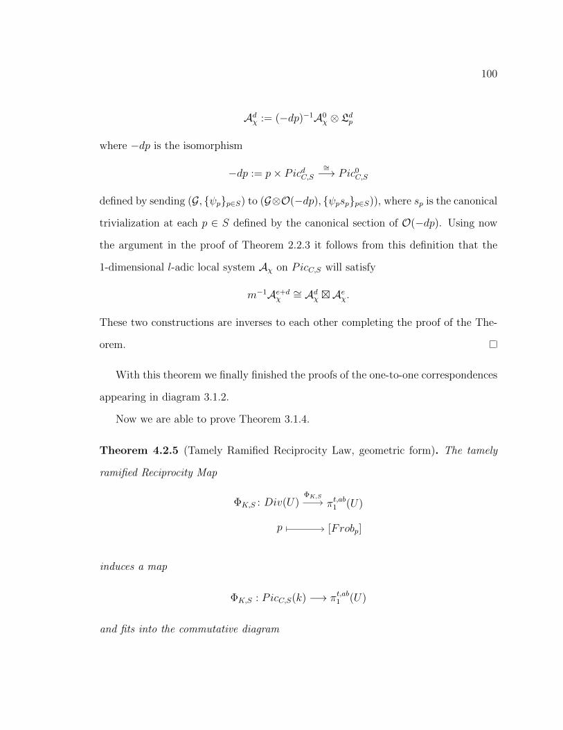
100

Adχ := (−dp)−1A0χ ⊗ Ldp

where −dp is the isomorphism

−dp := p× PicdC,S∼=−→ Pic0

C,S

defined by sending (G, ψpp∈S) to (G⊗O(−dp), ψpspp∈S)), where sp is the canonical

trivialization at each p ∈ S defined by the canonical section of O(−dp). Using now

the argument in the proof of Theorem 2.2.3 it follows from this definition that the

1-dimensional l-adic local system Aχ on PicC,S will satisfy

m−1Ae+dχ∼= Adχ Aeχ.

These two constructions are inverses to each other completing the proof of the The-

orem.

With this theorem we finally finished the proofs of the one-to-one correspondences

appearing in diagram 3.1.2.

Now we are able to prove Theorem 3.1.4.

Theorem 4.2.5 (Tamely Ramified Reciprocity Law, geometric form). The tamely

ramified Reciprocity Map

ΦK,S : Div(U) πt,ab1 (U)

p [Frobp]

ΦK,S

induces a map

ΦK,S : PicC,S(k) −→ πt,ab1 (U)

and fits into the commutative diagram

101

Pic0C,S(k) PicC,S(k) Z

Ker(ϕ) πt,ab1 (U) Z

deg

ϕ

ΦK,S can

such that there is an induced isomorphism on the kernels

Pic0C,S(k)

∼=−→ Ker(ϕ).

Proof. First we prove that the homomorphism

Div(U) −→ πt,ab1 (U)

induces a homomorphism

ΦK,S : PicC,S(k) −→ πt,ab1 (U).

For that let us take a continuous, 1-dimensional l-adic representation

χ : πt,ab1 (U) −→ Q×l .

By the geometric constructions we carried out and appearing in diagram 3.1.2, we can

associate to χ a 1-dimensional l-adic local system L on U which is tame at S, such

that for a closed point p : Spec(Fqn) −→ U , the Frobenius element Frobp acts on the

fibre Lp by multiplication by χ([Frobp]) ∈ Q×l . By Theorem 4.2.1 we can associate

to L a rigid multiplicative 1-dimensional l-adic local system AL on PicC,S and by

the faisceaux-fonctions correspondence we can associate to AL a 1-dimensional l-adic

representation

ψ : Pic0C,S(k) −→ Q×l

together with a Frobenius action Frobx : Z −→ Q×l , where x ∈ U(k). The pair

(ψ, Frobx) induces a 1-dimensional l-adic representation (using the same notation)

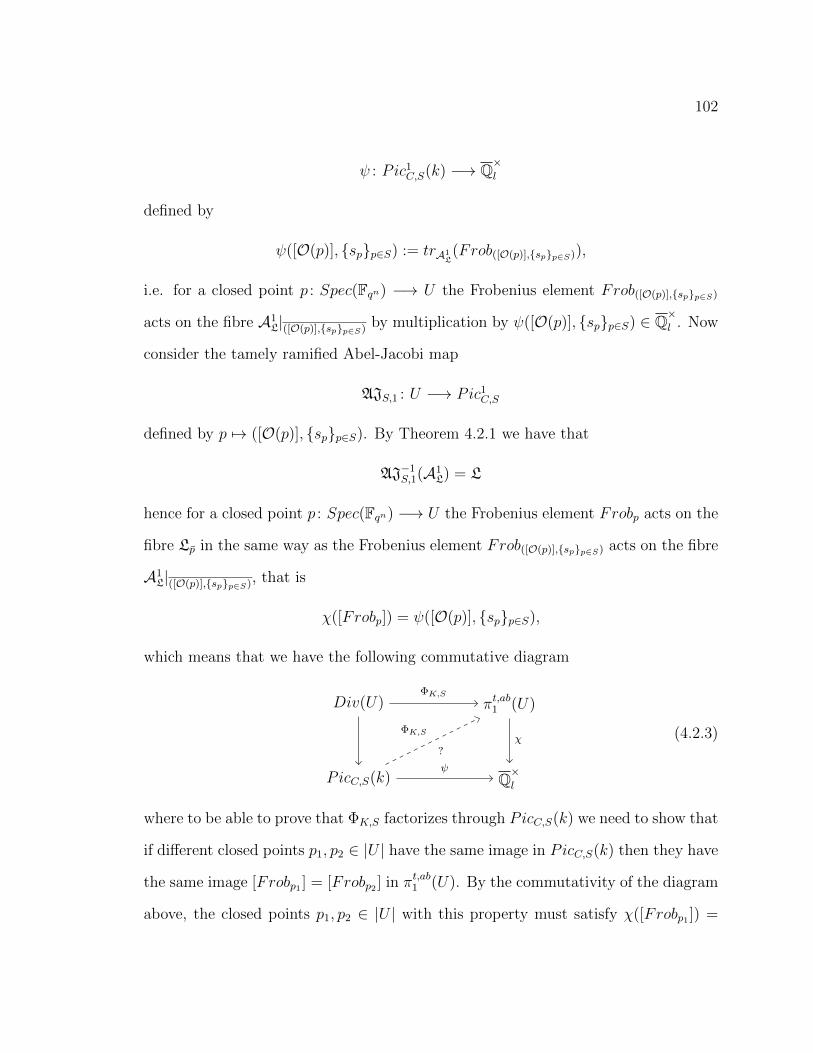
102

ψ : Pic1C,S(k) −→ Q×l

defined by

ψ([O(p)], spp∈S) := trA1L(Frob([O(p)],spp∈S)),

i.e. for a closed point p : Spec(Fqn) −→ U the Frobenius element Frob([O(p)],spp∈S)

acts on the fibre A1L|([O(p)],spp∈S) by multiplication by ψ([O(p)], spp∈S) ∈ Q×l . Now

consider the tamely ramified Abel-Jacobi map

AJS,1 : U −→ Pic1C,S

defined by p 7→ ([O(p)], spp∈S). By Theorem 4.2.1 we have that

AJ−1S,1(A1

L) = L

hence for a closed point p : Spec(Fqn) −→ U the Frobenius element Frobp acts on the

fibre Lp in the same way as the Frobenius element Frob([O(p)],spp∈S) acts on the fibre

A1L|([O(p)],spp∈S), that is

χ([Frobp]) = ψ([O(p)], spp∈S),

which means that we have the following commutative diagram

Div(U) πt,ab1 (U)

PicC,S(k) Q×l

ΦK,S

ψ

χΦK,S

?

(4.2.3)

where to be able to prove that ΦK,S factorizes through PicC,S(k) we need to show that

if different closed points p1, p2 ∈ |U | have the same image in PicC,S(k) then they have

the same image [Frobp1 ] = [Frobp2 ] in πt,ab1 (U). By the commutativity of the diagram

above, the closed points p1, p2 ∈ |U | with this property must satisfy χ([Frobp1 ]) =

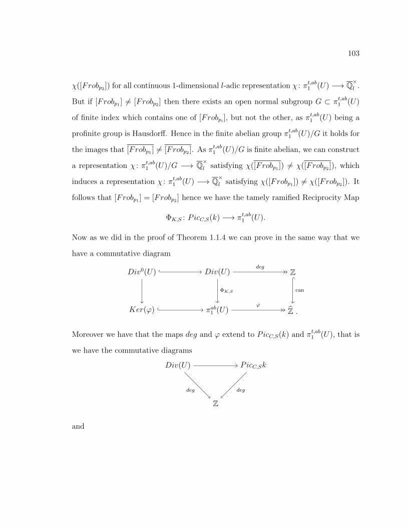
103

χ([Frobp2 ]) for all continuous 1-dimensional l-adic representation χ : πt,ab1 (U) −→ Q×l .

But if [Frobp1 ] 6= [Frobp2 ] then there exists an open normal subgroup G ⊂ πt,ab1 (U)

of finite index which contains one of [Frobpi ], but not the other, as πt,ab1 (U) being a

profinite group is Hausdorff. Hence in the finite abelian group πt,ab1 (U)/G it holds for

the images that [Frobp1 ] 6= [Frobp2 ]. As πt,ab1 (U)/G is finite abelian, we can construct

a representation χ : πt,ab1 (U)/G −→ Q×l satisfying χ([Frobp1 ]) 6= χ([Frobp2 ]), which

induces a representation χ : πt,ab1 (U) −→ Q×l satisfying χ([Frobp1 ]) 6= χ([Frobp2 ]). It

follows that [Frobp1 ] = [Frobp2 ] hence we have the tamely ramified Reciprocity Map

ΦK,S : PicC,S(k) −→ πt,ab1 (U).

Now as we did in the proof of Theorem 1.1.4 we can prove in the same way that we

have a commutative diagram

Div0(U) Div(U) Z

Ker(ϕ) πab1 (U) Z .

deg

ϕ

ΦK,S can

Moreover we have that the maps deg and ϕ extend to PicC,S(k) and πt,ab1 (U), that is

we have the commutative diagrams

Div(U) PicC,Sk

Z

degdeg

and

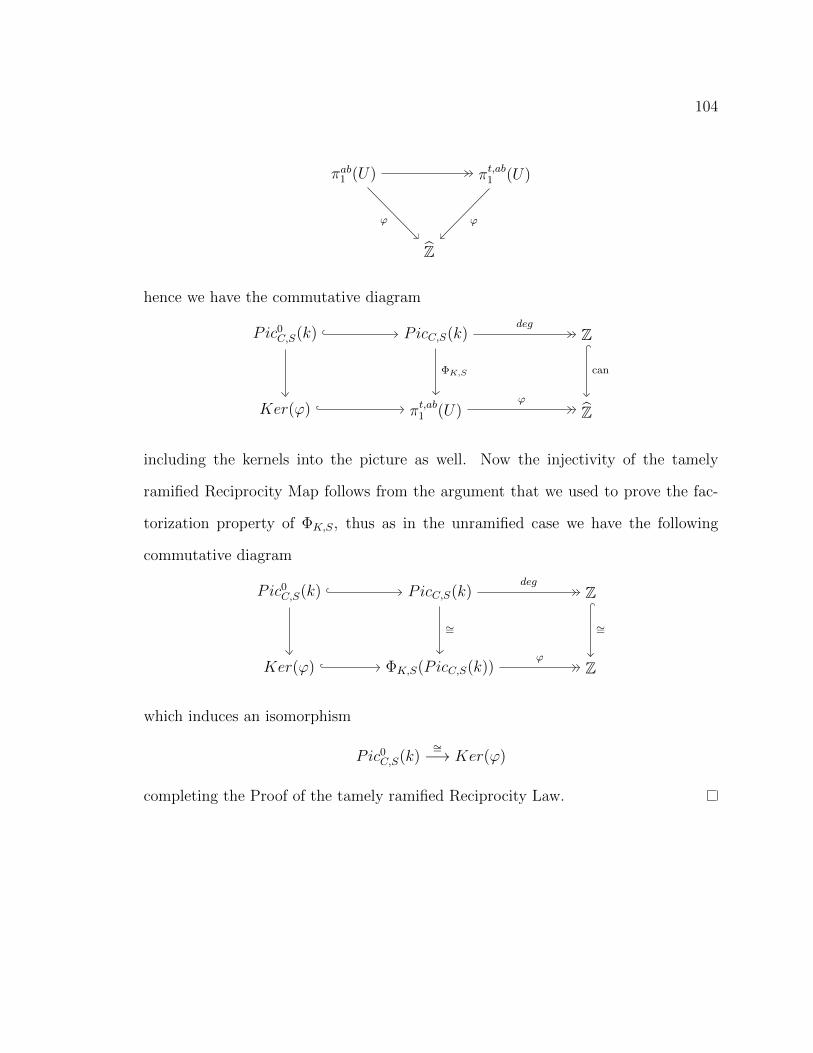
104

πab1 (U) πt,ab1 (U)

Z

ϕϕ

hence we have the commutative diagram

Pic0C,S(k) PicC,S(k) Z

Ker(ϕ) πt,ab1 (U) Z

deg

ϕ

ΦK,S can

including the kernels into the picture as well. Now the injectivity of the tamely

ramified Reciprocity Map follows from the argument that we used to prove the fac-

torization property of ΦK,S, thus as in the unramified case we have the following

commutative diagram

Pic0C,S(k) PicC,S(k) Z

Ker(ϕ) ΦK,S(PicC,S(k)) Z

deg

ϕ

∼= ∼=

which induces an isomorphism

Pic0C,S(k)

∼=−→ Ker(ϕ)

completing the Proof of the tamely ramified Reciprocity Law.

Bibliography

[AM69] M.F. Atiyah and I.G. Macdonald. Introduction to Commutative Algebra.

Addison-Wesley Publishing Company, London, 1969.

[AT90] E. Artin and J. Tate. Class Field Theory. Addison-Wesley Publishing

Company, London, 1990.

[Del77] P. Deligne. Cohomologie Etale, SGA 412. Springer Verlag, Berlin, New York,

1977.

[FK88] E. Freitag and R. Kiel. Etale Cohomology and the Weil Conjecture.

Springer-Verlag, Berlin Heidelberg, 1988.

[Fre05] E. Frenkel. Lectures on the Langlands Program and Conformal Field The-

ory. http://arxiv.org/PS_cache/hep-th/pdf/0512/0512172v1.pdf,

2005.

[Gai04] D. Gaitsgory. Informal Introduction to Geometric Langlands. In J. Bern-

stein and S. Gelbart, editors, An Introduction to the Langlands Program.

Birkhauser Boston, 2004.

[GM71] A. Grothendieck and J.P. Murre. The Tame Fundamental Group of a

Formal Neighborhood of a Divisor with Normal Crossings on a Scheme.

Springer Verlag, Berlin Heidelberg New York, 1971.

105

106

[Gro61] A. Grothendieck. Revetements etale et Groupe Fondamental (SGA 1).

http://library.msri.org/books/sga/sga/ps/index.html, 1960-61.

[Gro66] A. Grothendieck. Cohomologie l-adique et Fonctions L (SGA 5). http:

//library.msri.org/books/sga/sga5/index.html, 1965-66.

[Har06] R. Hartshorne. Algebraic Geometry. Springer Science + Business Media,

LLC, New York, 2006.

[Hei04] J. Heinloth. Wenig Verzweigte Geometrische Langlands-Korrespondenz.

In Y. Tschinkel, editor, Gottingen Seminars WS03-04. Universitatsverlag

Gottingen, 2004.

[Hei07] J. Heinloth. Class Field Theory. In Geometric Langlands Program winter

school in Gottingen, 2007.

[Lau90] G. Laumon. Faisceaux Automorphes Lies aux Series Eisenstein. In L. Clozel

and J.S. Milne, editors, Automorphic Forms, Shimura Varieties and L-

functions. Academic Press, 1990.

[Liu02] Q. Liu. Algebraic Geometry and Arithmetic Curves. Oxford University

Press Inc., New York, 2002.

[Mil80] J.S. Milne. Etale Cohomology. Princeton University Press, Princeton, New

Yersey, 1980.

[Mil08a] J.S. Milne. Abelian Varieties. http://www.jmilne.org/math/

CourseNotes/av.html, 2008. lecture notes.

[Mil08b] J.S. Milne. Class Field Theory. http://www.jmilne.org/math/

CourseNotes/cft.html, 2008. lecture notes.

[Mil08c] J.S. Milne. Lectures on etale Cohomology. http://www.jmilne.org/math/

CourseNotes/lec.html, 2008. lecture notes.

107

[Mum70] D. Mumford. Abelian Varieties. Oxford University Press (Tata Institute),

Oxford, Bombay, 1970.

[Neu07] J. Neukirch. Algebraische Zahlentheorie. Springer Verlag, Berlin Heidelberg,

2007.

[RZ00] L. Ribes and P. Zalesskii. Profinite Groups. Springer Verlag, Berlin Hei-

delberg, 2000.

[Sch05] A. Schmidt. Higher Dimensional Class Field Theory. http://www.mathi.

uni-heidelberg.de/~schmidt/papers/schmidt21-de.html, 2005.

[Ser88] J-P. Serre. Algebraic Groups and Class Fields. Springer Verlag, New York,

1988.

[Shi05] Sug Woo Shin. Grothendieck Function-Sheaf Correspondence. http://

www-personal.umich.edu/~jkass/files/FS.pdf, Oktober 2005.

[SS99] A. Schmidt and M. Spieß. Singular Homology and Class Field Theory

of Varieties over Finite Fields. http://www.mathi.uni-heidelberg.de/

~schmidt/papers/schmidt12-de.html, 1999.

[Sza09a] T. Szamuely. Corps de Classes des Schemas Field Arithmetiques. http:

//www.renyi.hu/~szamuely/publ.html, 2009.

[Sza09b] T. Szamuely. Galois Groups and Fundamental Groups. Cambridge Univer-

sity Press, Cambridge, 2009.