geometric optimization in machine learning - suvritsuvrit.de/papers/sra_hosseini_chapter.pdf ·...

Geometric Optimization in Machine Learning

Suvrit Sra and Reshad Hosseini

Abstract Machine learning models often rely on sparsity, low-rank, orthogonality,correlation, or graphical structure. The structure of interest in this chapter is geomet-ric, specifically the manifold of positive definite (PD) matrices. Though these matri-ces recur throughout the applied sciences, our focus is on more recent developmentsin machine learning and optimization. In particular, we study (i) models that mightbe nonconvex in the Euclidean sense but are convex along the PD manifold; and (ii)ones that are fully nonconvex but are nevertheless amenable to global optimization.We cover basic theory for (i) and (ii); subsequently, we present a scalable Rieman-nian limited-memory BFGS algorithm (that also applies to other manifolds). Wehighlight some applications from statistics and machine learning that benefit fromthe geometric structure studies.

1 Introduction

Fitting mathematical models to data invariably requires numerical optimization.The field is thus replete with tricks and techniques for better modeling, analysis,and implementation of optimization algorithms. Among other aspects, the notion of“structure,” is of perennial importance: its knowledge often helps us obtain fasteralgorithms, permit scalability, gain insights, or capture a host of other attributes.

Structure has multifarious meanings, of which perhaps the best known is spar-sity [5, 52]. But our focus is different: we study geometric structure, in particularwhere model parameters lie on a Riemannian manifold.

Suvrit SraMassachusetts Institute of Technology, Cambridge, MA, USA e-mail: [email protected]

Reshad HosseiniSchool of ECE, College of Engineering, University of Tehran, Tehran, Iran e-mail: [email protected]

1

2 Suvrit Sra and Reshad Hosseini

Geometric structure has witnessed increasing interest, for instance in optimiza-tion over matrix manifolds (including orthogonal, low-rank, positive definite matri-ces, among others) [1, 12, 50, 55]. However, in distinction to general manifold opti-mization, which extends most Euclidean schemes to Riemannian manifolds [1, 53],we focus on specific case of “geometric optimization” problems that exploit thespecial structure of the manifold of positive definite (PD) matrices. Two geomet-ric aspects play a crucial role here: (i) the nonpositive curvature of the manifold,which allows defining a global curved notion of convexity along geodesics on themanifold; and (ii) the convex (Euclidean) conic structure (e.g., as used in Perron-Frobenius theory, which includes the famous PageRank algorithm as a special case).

One of our key motivations for studying geometric optimization is that for manyproblems it may help uncover hidden (geodesic) convexity, and thus provably placeglobal optimization of certain nonconvex problems within reach [50]. Moreover,exploiting geometric convexity can have remarkable empirical consequences forproblems involving PD matrices [47]; which persist even without overall (geodesic)convexity, as will be seen in §3.1.

Finally, since PD matrices are ubiquitous in not only machine learning and statis-tics, but throughout the applied sciences, the new modeling and algorithmic tools of-fered by geometric optimization should prove to be valuable in many other settings.To stoke the reader’s imagination beyond the material described in this chapter, weclose with a short list of further applications in Section 3.3. We also refer the readerto our recent work [50], that develops the theoretical material related to geometricoptimization in greater detail.

With this background, we are now ready to recall the geometric concepts at theheart of our presentation, before moving on to detailed applications of our ideas.

1.1 Manifolds and Geodesic Convexity

A smooth manifold is a space that locally resembles Euclidean space [29]. We focuson Riemannian manifolds (smooth manifolds equipped with a smoothly varyinginner product on the tangent space) as their geometry permits a natural extension ofmany nonlinear optimization algorithms [1, 53].

In particular, we focus on the (matrix) manifold of real symmetric positive def-inite (PD) matrices. Most of the ideas that we describe apply more broadly toHadamard manifolds (i.e., Riemannian manifolds with non-positive curvature), butwe limit attention to the PD manifold for concreteness and due to its vast importancein machine learning and beyond [6, 17, 45].

A key concept on manifolds is that of geodesics which are curves that join pointsalong shortest paths. Geodesics help one extend the notion of convexity to geodesicconvexity. Formally, suppose M is a Riemmanian manifold, and x,y are two pointson M . Say γ is a unit speed geodesic joining x to y, such that

γxy : [0,1]→M , s.t. γxy(0) = x, γxy(1) = y.

Geometric Optimization in Machine Learning 3

Then, we call a set A ⊆ M geodesically convex, henceforth g-convex, if thegeodesic joining an arbitrary pair of points in A lies completely in A . We sayf : A → R is g-convex if for all x,y ∈ A , the composition f ◦ γxy : [0,1]→ R isconvex in the usual sense. For example, on the manifold Pd of d× d PD matricesthe geodesic γXY between X ,Y ∈ Pd has the beautiful closed-form [6, Ch. 6]:

γXY (t) := X1/2(X−1/2Y X−1/2)tX1/2, 0≤ t ≤ 1. (1)

It is common to write X]tY ≡ γXY (t), and we also use this notation for brevity.Therewith, a function f : Pd → R is g-convex if on a g-convex set A it satisfies

f (X]tY )≤ (1− t) f (X)+ t f (Y ), t ∈ [0,1], X ,Y ∈A . (2)

G-convex functions are remarkable in that they can be nonconvex in the Euclideansense, but can still be globally optimized. Such functions on PD matrices have al-ready proved important in several recent applications [17,18,23,44,48,49,57,58,62].We provide below several examples, and refer the interested reader to our work [50]for a detailed, more systematic development of g-convexity on PD matrices.

Example 1 ( [50]). The following functions are g-convex on Pd : (i) tr(eA); (ii) tr(Aα)

for α ≥ 1; (iii) λ↓1 (e

A); (iv) λ↓1 (A

α) for α ≥ 1.

Example 2 ( [50]). Let X ∈ Cd×k be an arbitrary rank-k matrix (k ≤ d), then A 7→trX∗AX is log-g-convex, that is,

trX∗(A]tB)X ≤ [trX∗AX ]1−t [trX∗BX ]t , t ∈ [0,1]. (3)

Inequality (3) depends on a nontrivial property of ]t proved e.g., in [50, Thm. 2.8].

Example 3. If h : R+ → R+ is nondecreasing and log-convex, then the map A 7→∑

ki=1 logh(λi(A)) is g-convex. For instance, if h(x) = ex, we obtain the special case

that A 7→ log tr(eA) is g-convex.

Example 4. Let Ai ∈ Cd×k with k ≤ d such that rank([Ai]mi=1) = k; also let B � 0.

Then φ(X) := logdet(B+∑i A∗i XAi) is g-convex on Pd .

Example 5. The Riemannian distance δR(A,X) := ‖log(X−1/2AX−1/2)‖F betweenA,X ∈ Pd [6, Ch. 6] is well-known to be jointly g-convex, see e.g., [6, Cor. 6.1.11].To obtain an infinite family of such g-convex distances see [50, Cor. 2.19].

Consequently, the Frechet (Karcher) mean and median of PD matrices are g-convex optimization problems. Formally, these problems seek to solve

minX�0

∑mi=1 wiδR(X ,Ai), (Geometric Median),

minX�0

∑mi=1 wiδ

2R(X ,Ai), (Geometric Mean),

where ∑i wi = 1, wi ≥ 0, and Ai � 0 for 1≤ i≤ m. The latter problem has receivedextensive interest in the literature [6–8,25,39,41,48]. Its optimal solution is uniqueowing to the strict g-convexity of its objective.


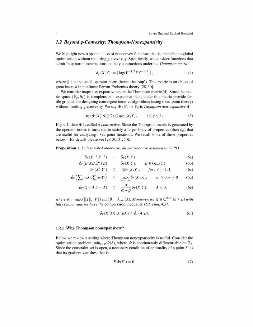
1.2 Beyond g-Convexity: Thompson-Nonexpansivity

We highlight now a special class of nonconvex functions that is amenable to globaloptimization without requiring g-convexity. Specifically, we consider functions thatadmit “sup norm” contractions, namely contractions under the Thompson metric:

δT (X ,Y ) := ‖log(Y−1/2XY−1/2)‖, (4)

where ‖·‖ is the usual operator norm (hence the ‘sup’). This metric is an object ofgreat interest in nonlinear Perron-Frobenius theory [28, 30].

We consider maps non-expansive under the Thompson metric (4). Since the met-ric space (Pd ,δT ) is complete, non-expansive maps under this metric provide fer-tile grounds for designing convergent iterative algorithms (using fixed-point theory)without needing g-convexity. We say Φ : Pd → Pd is Thompson non-expansive if

δT (Φ(X),Φ(Y ))≤ qδT (X ,Y ), 0≤ q≤ 1. (5)

If q < 1, then Φ is called q-contractive. Since the Thompson metric is generated bythe operator norm, it turns out to satisfy a larger body of properties (than δR) thatare useful for analyzing fixed-point iterations. We recall some of these propertiesbelow—for details please see [28, 30, 31, 50].

Proposition 1. Unless noted otherwise, all matrices are assumed to be PD.

δT (X−1,Y−1) = δT (X ,Y ) (6a)δT (B∗XB,B∗Y B) = δT (X ,Y ), B ∈ GLn(C) (6b)

δT (X t ,Y t) ≤ |t|δT (X ,Y ), for t ∈ [−1,1] (6c)

δT

(∑i wiXi,∑i wiYi

)≤ max

1≤i≤mδT (Xi,Yi), wi ≥ 0,w 6= 0 (6d)

δT (X +A,Y +A) ≤ α

α +βδT (X ,Y ), A� 0, (6e)

where α = max{‖X‖,‖Y‖} and β = λmin(A). Moreover, for X ∈ Cd×k (k ≤ d) withfull column rank we have the compression inequality [50, Thm. 4.3]:

δT (X∗AX ,X∗BX)≤ δT (A,B). (6f)

1.2.1 Why Thompson nonexpansivity?

Below we review a setting where Thompson nonexpansivity is useful. Consider theoptimization problem: minS�0 Φ(S), where Φ is continuously differentiable on Pd .Since the constraint set is open, a necessary condition of optimality of a point S∗ isthat its gradient vanishes, that is,

∇Φ(S∗) = 0. (7)


Various approaches could be used for solving the nonlinear (matrix) equation (7).And among these, fixed-point iterations may be particularly attractive. Here, onedesigns a map G : Pd → Pd , using which we can rewrite (7) in the form

S∗ = G (S∗), (8)

that is, S∗ is a fixed-point of G , and by construction a stationary point of Φ .Typically, finding fixed-points is difficult. However, if the map G can be chosen

such that it is Thompson contractive, then simply running the Picard iteration

Sk+1← G (Sk), k = 0,1, . . . , (9)

will yield a unique solution to (7)—both existence and uniqueness follow from theBanach contraction theorem. The reason we insist on Thompson contractivity is be-cause many of our examples fail to be Euclidean contractions (or even Riemanniancontractions) but end up being Thompson contractions. Thus, studying Thompsonnonexpansivity is valuable. We highlight below a concrete example that arises insome applications [15–18, 61], and is not a Euclidean but a Thompson contraction.

Application: Geometric Mean of PD Matrices.

Let A1, . . . ,An ∈ Pd be input matrices and wi ≥ 0 be nonnegative weights suchthat ∑

ni=1 wi = 1. A particular geometric mean of the {Ai}n

i=1, called the S-mean, isobtained by computing [15, 18]

minX�0

h(X) := ∑ni=1 wiδ

2S (X ,Ai), (10)

where δ 2S is the squared Stein-distance

δ2S (X ,Y ) := logdet

(X+Y2

)− 1

2 logdet(XY ), X ,Y � 0. (11)

It can be shown that δ 2S is strictly g-convex (in both arguments) [48]. Thus, Prob-

lem (10) is a g-convex optimization problem. It is easily seen to possess a solution,whence the strict g-convexity of h(X) immediately implies that this solution mustbe unique. What remains is to obtain an algorithm to compute this solution.

Following (7), we differentiate h(X) and obtain the nonlinear matrix equation

0 = ∇h(X)≡ X−1 = ∑i wi

(X+Ai

2

)−1,

from which we naively obtain the Picard iteration

Xk+1←[∑i wi

(Xk+Ai

2

)−1]−1. (12)

Applying (6a), (6d), and (6e) in sequence we see that (12) is Thompson contraction,which immediately allows us to conclude its validity as a Picard iteration and itslinear rate of convergence (in the Thompson metric) to the global optimum of (10).


2 Manifold Optimization

Creating fixed-point iterations is somewhat of an art, and it is not always clear howto obtain one for a given problem. Therefore, developing general purpose iterativeoptimization algorithms is of great practical importance.

For Euclidean optimization a common recipe is to iteratively (a) find a descentdirection; and (b) obtain sufficient decrease via line-search which also helps ensureconvergence. We follow a similar recipe for Riemannian manifolds by replacing Eu-clidean concepts by their Riemannian counterparts. For example, we now computedescent directions in the tangent space. At a point X , the tangent space TX is theapproximating vector space (see Fig. 1). Given a descent direction ξX ∈ TX , we per-form line-search along a smooth curve on the manifold (red curve in Fig. 1). Thederivative of this curve at X provides the descent direction ξX . We refer the readerto [1, 53] for an in depth introduction to manifold optimization.

Sd+

X

TX

⇠X

Fig. 1 Line-search on a manifold: X is apoint on the manifold, TX is the tangentspace at the point X , ξX is a descent direc-tion at X ; the red curve is the curve alongwhich line-search is performed.

Euclidean methods such as conjugate-gradient and LBFGS combine gradients at thecurrent point with gradients and descent di-rections at previous points to obtain a newdescent direction. To adapt such algorithmsto manifolds we need to define how to trans-port vectors in a tangent space at one point tovectors in a tangent space at another point.

On Riemannian manifolds, the gradient isa direction in the tangent space, where theinner-product of the gradient with another di-rection in the tangent space gives the direc-tional derivative of the function. Formally, ifgX defines the inner product in the tangentspace TX , then

D f (X)ξ = gX (grad f (X),ξ ), for ξ ∈ TX .

Given a descent direction the curve along which we perform line-search can bea geodesic. A map that combines the direction and a step-size to obtain a corre-sponding point on the geodesic is called an exponential map. Riemannian mani-folds also come equipped with a natural way to transport vectors on geodesics thatis called parallel transport. Intuitively, a parallel transport is a differential map withzero derivative along the geodesics.

Using these ideas, and in particular deciding where to perform the vector trans-port we can obtain different variants of Riemannian LBFGS. We recall one specificLBFGS variant from [50] (presented as Alg. 1), which yields the best performancein our applications, once we combine it with a suitable line-search algorithm.

In particular, to ensure Riemannian LBFGS always produces a descent direction,we must ensure that the line-search algorithm satisfies the Wolfe conditions [44]:


Table 1 Summary of key Riemannian objects for the PD matrix manifold.

Definition Expression for PD matricesTangent space Space of symmetric matrices

Metric between two tangent vectors ξ ,η at Σ gΣ (ξ ,η) = tr(Σ−1ξ Σ−1η)Gradient at Σ if Euclidean gradient is ∇ f (Σ) grad f (Σ) = 1

2 Σ(∇ f (X)+∇ f (X)T )ΣExponential map at point Σ in direction ξ RΣ (ξ ) = Σ exp(Σ−1ξ )

Parallel transport of tangent vector ξ from Σ1 to Σ2 TΣ1,Σ2 (ξ ) = Eξ ET , E = (Σ2Σ−11 )1/2

f (RXk(αξk))≤ f (Xk)+ c1αD f (Xk)ξk, (13)D f (Xk+1)ξk+1 ≥ c2D f (Xk)ξk, (14)

where 0< c1 < c2 < 1. Note that αD f (Xk)ξk = gXk(grad f (Xk),αξk), i.e., the deriva-tive of f (Xk) in the direction αξk is the inner product of descent direction and gra-dient of the function. Practical line-search algorithms implement a stronger (Wolfe)version of (14) that enforces

|D f (Xk+1)ξk+1| ≤ c2D f (Xk)ξk. (15)

Key details of a practical way to implement this line-search may be found in [23].

Algorithm 1 Pseudocode for Riemannian LBFGSGiven: Riemannian manifold M with Riemannian metric g; parallel transport T on M ;geodesics R; initial value X0; a smooth function fSet initial Hdiag = 1/

√gX0 (grad f (X0),grad f (X0))

for k = 0,1, . . . doObtain descent direction ξk by unrolling the RBFGS methodCompute ξk← HESSMUL(−grad f (Xk),k)Use line-search to find α such that it satisfies Wolfe conditionsCalculate Xk+1 = RXk (αξk)Define Sk = TXk ,Xk+1 (αξk)Define Yk = grad f (Xk+1)−TXk ,Xk+1 (grad f (Xk))Update Hdiag = gXk+1 (Sk,Yk)/gXk+1 (Yk,Yk)Store Yk; Sk; gXk+1 (Sk,Yk); gXk+1 (Sk,Sk)/gXk+1 (Sk,Yk); Hdiag

end forreturn Xkfunction HESSMUL(P,k)if k > 0 then

Pk = P−gXk+1 (Sk ,Pk+1)

gXk+1 (Yk ,Sk)Yk

P = TXk+1,Xk HESSMUL(TXk ,Xk+1 Pk,k−1) return P−gXk+1 (Yk ,P)gXk+1 (Yk ,Sk)

Sk +gXk+1 (Sk ,Sk)

gXk+1 (Yk ,Sk)P

elsereturn HdiagP

end ifend function


3 Applications

We are ready to present two applications of geometric optimization. Section 3.1summarizes recent progress in fitting Gaussian Mixture Models (GMMs), for whichg-convexity proves remarkably useful and ultimately helps Alg. 1 to greatly outper-form the famous Expectation Maximization (EM) algorithm—this is remarkable aspreviously many believed it impossible to outdo EM via general nonlinear optimiza-tion techniques. Next, in Section 3.2 we present an application to maximum like-lihood parameter estimation for non-Gaussian elliptically contoured distributions.These problems are Euclidean nonconvex but often either g-convex or Thompsonnonexpansive, and thus amenable to geometric optimization.

3.1 Gaussian Mixture Models

This material of this section is based on the authors’ recent work [23]; the interestedreader is encouraged to consult that work for additional details.

Gaussian Mixture Models (GMMs) have a long history in machine learning andsignal processing and continue to enjoy widespread use [10, 21, 36, 40]. For GMMparameter estimation, Expectation Maximization (EM) [20] still seems to be the defacto choice—although other approaches have also been considered [43], typicalnonlinear programming methods such as conjugate gradients, quasi-Newton, New-ton, are usually viewed as inferior to EM [59].

One advantage that EM enjoys is that its M-Step satisfies the PD constraint oncovariances by construction. Other methods often struggle when dealing with thisconstraint. An approach is to make the problem unconstrained by performing achange-of-variables using Cholesky decompositions (as also exploited in semidefi-nite programming [14]). Another possibility is to formulate the PD constraint via aset of smooth convex inequalities [54] or to use log-barriers and to invoke interior-point methods. But such methods tend to be much slower than EM-like iterations,especially in higher dimensions [49].

Driven by these concerns the authors view GMM fitting as a manifold optimiza-tion problem in [23]. But surprisingly, an out-of-the-box invocation of manifoldoptimization completely fails! To compete with and to outdo EM, further work isrequired: g-convexity supplies the missing link.

3.1.1 Problem Setup

Let N denote the Gaussian density with mean µ ∈ Rd and covariance Σ ∈ Pd , i.e.,

N (x; µ,Σ) := det(Σ)−1/2(2π)−d/2 exp(− 1

2 (x−µ)TΣ−1(x−µ)

).

A Gaussian Mixture Model has the probability density


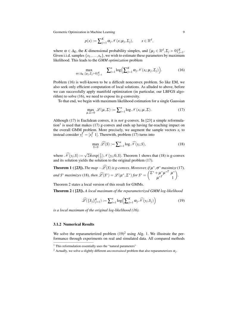
p(x) := ∑Kj=1 α jN (x; µ j,Σ j), x ∈ Rd ,

where α ∈ ∆K , the K-dimensional probability simplex, and {µ j ∈ Rd ,Σ j � 0}Kj=1.

Given i.i.d. samples {x1, . . . ,xn}, we wish to estimate these parameters by maximumlikelihood. This leads to the GMM optimization problem

maxα∈∆K ,{µ j ,Σ j�0}Kj=1

∑ni=1 log

(∑

Kj=1 α jN (xi; µ j,Σ j)

). (16)

Problem (16) is well-known to be a difficult nonconvex problem. So like EM, wealso seek only efficient computation of local solutions. As alluded to above, beforewe can successfully apply manifold optimization (in particular, our LBFGS algo-rithm) to solve (16), we need to expose its g-convexity.

To that end, we begin with maximum likelihood estimation for a single Gaussian

maxµ,Σ�0

L (µ,Σ) := ∑ni=1 logN (xi; µ,Σ). (17)

Although (17) is Euclidean convex, it is not g-convex. In [23] a simple reformula-tion1 is used that makes (17) g-convex and ends up having far-reaching impact onthe overall GMM problem. More precisely, we augment the sample vectors xi toinstead consider yT

i = [xTi 1]. Therewith, problem (17) turns into

maxS�0

L (S) := ∑ni=1 logN (yi;S), (18)

where N (yi;S) :=√

2π exp( 12 )N (yi;0,S). Theorem 1 shows that (18) is g-convex

and its solution yields the solution to the original problem (17).

Theorem 1 ( [23]). The map−L (S) is g-convex. Moreover, if µ∗,σ∗ maximize (17),

and S∗ maximizes (18), then L (S∗) = L (µ∗,Σ ∗) for S∗ =(

Σ ∗+µ∗µ∗Tµ∗

µ∗T 1

).

Theorem 2 states a local version of this result for GMMs.

Theorem 2 ( [23]). A local maximum of the reparameterized GMM log-likelihood

L ({S j}Kj=1) := ∑

ni=1 log

(∑

Kj=1 α jN (yi;S j)

)(19)

is a local maximum of the original log-likelihood (16).

3.1.2 Numerical Results

We solve the reparameterized problem (19)2 using Alg. 1. We illustrate the per-formance through experiments on real and simulated data. All compared methods

1 This reformulation essentially uses the “natural parameters”2 Actually, we solve a slightly different unconstrained problem that also reparameterizes α j .


are initialized using k-means++ [3], and all share the same stopping criterion. Themethods stop when the difference of average log-likelihood (i.e., log-likelihood/n)between iterations falls below 10−6, or when the iteration count exceeds 1500.

Since EM’s performance depends on the degree of separation of the mixturecomponents [32, 59], we also assess the impact of separation on our methods. Wegenerate data as proposed in [19, 56]. The distributions are chosen so their meanssatisfy the following separation inequality:

∀i 6= j : ‖µi−µ j‖ ≥ cmaxi, j{tr(Σi), tr(Σ j)}.

The parameter c shows level of separation; we use e to denote eccentricity, i.e., theratio of the largest eigenvalue of the covariance matrix to its smallest eigenvalue. Atypical 2D data with K = 5 created for different separations is shown in Figure 2.

−1.5 −1 −0.5 0 0.5 1 1.5 2−1.5

−1

−0.5

0

0.5

1

1.5

2

(a) low separation−1 −0.5 0 0.5 1 1.5 2

−1

−0.5

0

0.5

1

1.5

2

2.5

(b) medium separation0 1 2 3 4 5 6 7

−1

0

1

2

3

4

5

6

7

8

(c) high separation

Fig. 2 Data clouds for three levels of separation: c = 0.2 (low); c = 1 (medium); c = 5 (high).

We tested both high eccentricity (e= 10) and spherical (e= 1) Gaussians. Table 2reports the results, which are obtained after running 20 different random initializa-tions. Without our reformulation Riemannian optimization is not competitive (weomit the results), while with the reformulation our Riemannian LBFGS matches orexceeds EM. We note in passing that a Cholesky decomposition based formulationends up being vastly inferior to both EM and our Riemannian methods. Numericalresults supporting this claim may be found in [23].

Table 2 Speed and average log-likelihood (ALL) comparisons for d = 20, e = 10 and e = 1. Thenumbers are averaged values for 20 runs over different sampled datasets, therefore the ALL valuesare not comparable to each other. The standard-deviation are also reported in the table.

EM (e = 10) LBFGS (e = 10) EM (e = 1) LBFGS (e = 1)Time (s) ALL Time (s) ALL Time (s) ALL Time (s) ALL

c = 0.2 K = 2 1.1 ± 0.4 -10.7 5.6 ± 2.7 -10.7 65.7 ± 33.1 17.6 39.4 ± 19.3 17.6K = 5 30.0 ± 45.5 -12.7 49.2 ± 35.0 -12.7 365.6 ± 138.8 17.5 160.9 ± 65.9 17.5

c = 1 K = 2 0.5 ± 0.2 -10.4 3.1 ± 0.8 -10.4 6.0 ± 7.1 17.0 12.9 ± 13.0 17.0K = 5 104.1 ± 113.8 -13.4 79.9 ± 62.8 -13.3 40.5 ± 61.1 16.2 51.6 ± 39.5 16.2

c = 5 K = 2 0.2 ± 0.2 -11.0 3.4 ± 1.4 -11.0 0.2 ± 0.1 17.1 3.0 ± 0.5 17.1K = 5 38.8 ± 65.8 -12.8 41.0 ± 45.7 -12.8 17.5 ± 45.6 16.1 20.6 ± 22.5 16.1


Table 3 Speed and ALL comparisons for natural image data d = 35.EM Algorithm LBFGS Reformulated CG Reformulated CG Original CG Cholesky ReformulatedTime (s) ALL Time (s) ALL Time (s) ALL Time (s) ALL Time (s) ALL

K = 2 16.61 29.28 14.23 29.28 17.52 29.28 947.35 29.28 476.77 29.28K = 4 165.77 31.65 106.53 31.65 153.94 31.65 6380.01 31.64 2673.21 31.65K = 8 596.01 32.81 332.85 32.81 536.94 32.81 14282.80 32.58 9306.33 32.81K = 10 2159.47 33.05 658.34 33.06 1048.00 33.06 17711.87 33.03 7463.72 33.05

Next, we present an evaluation on a natural image dataset, for which GMMs havebeen reported to be effective [64]. We extracted 200K image patches of size 6× 6from random locations in the images and subtracted the DC component. GMM fit-ting results obtained by different algorithms are reported in Table 3. As can be seen,manifold LBFGS performs better than EM and manifold CG. Moreover, our refor-mulation proves crucial: without it manifold optimization is substantially slower.The Cholesky-based model without our reformulation has the worst performance(not reported), and even with reformulation it is inferior to the other approaches.

Fig. 3 visualizes evolution of the objective function with the number of iterations(i.e., the number of log-likelihood and gradient evaluations, or the number of E- andM-steps). The datasets used in Fig. 3 are the ‘magic telescope’ and ‘year prediction’datasets3, as well as natural image data used in Table 2. It can be seen that althoughmanifold optimization methods spend time doing line-search they catch up with EMalgorithm in a few iterations.

0 50 100 150 200 250 30010−5

10−4

10−3

10−2

10−1

100

101

102

# function and gradient evaluations

AL

L∗

-AL

L

EM, Usual MVNLBFGS, Reparameterized MVNCG, Reparameterized MVN

0 50 100 150 20010−5

10−4

10−3

10−2

10−1

100

101

102


AL

L∗

-AL

L

EM, Original MVNLBFGS, Reformulated MVNCG, Reformulated MVN

0 50 100 150 200 25010−5

10−4

10−3

10−2

10−1

100

101

102


AL

L∗

-AL

L

EM, Original MVNLBFGS, Reformulated MVNCG, Reformulated MVN

Fig. 3 The objective function with respect to the number of function and gradient evaluations. Theobjective function is the Best ALL minus current ALL values. Left: ‘magic telescope’ (K = 5,d =10). Middle: ‘year predict’ (K = 6,d = 90). Right: natural images (K = 8,d = 35).

3.2 MLE for Elliptically Contoured Distributions

Our next application is to maximum likelihood parameter estimation for Kotz-typedistributions. Here given i.i.d. samples (x1, . . . ,xn) from an Elliptically ContouredDistribution Eϕ(S), up to constants the log-likelihood is of the form

3 Available at UCI machine learning dataset repository via https://archive.ics.uci.edu/ml/datasets


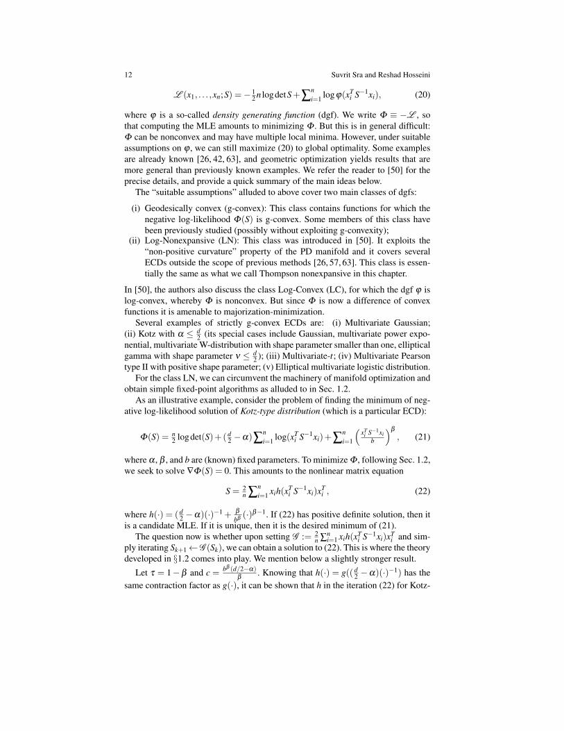
L (x1, . . . ,xn;S) =− 12 n logdetS+∑

ni=1 logϕ(xT

i S−1xi), (20)

where ϕ is a so-called density generating function (dgf). We write Φ ≡ −L , sothat computing the MLE amounts to minimizing Φ . But this is in general difficult:Φ can be nonconvex and may have multiple local minima. However, under suitableassumptions on ϕ , we can still maximize (20) to global optimality. Some examplesare already known [26, 42, 63], and geometric optimization yields results that aremore general than previously known examples. We refer the reader to [50] for theprecise details, and provide a quick summary of the main ideas below.

The “suitable assumptions” alluded to above cover two main classes of dgfs:

(i) Geodesically convex (g-convex): This class contains functions for which thenegative log-likelihood Φ(S) is g-convex. Some members of this class havebeen previously studied (possibly without exploiting g-convexity);

(ii) Log-Nonexpansive (LN): This class was introduced in [50]. It exploits the“non-positive curvature” property of the PD manifold and it covers severalECDs outside the scope of previous methods [26, 57, 63]. This class is essen-tially the same as what we call Thompson nonexpansive in this chapter.

In [50], the authors also discuss the class Log-Convex (LC), for which the dgf ϕ islog-convex, whereby Φ is nonconvex. But since Φ is now a difference of convexfunctions it is amenable to majorization-minimization.

Several examples of strictly g-convex ECDs are: (i) Multivariate Gaussian;(ii) Kotz with α ≤ d

2 (its special cases include Gaussian, multivariate power expo-nential, multivariate W-distribution with shape parameter smaller than one, ellipticalgamma with shape parameter ν ≤ d

2 ); (iii) Multivariate-t; (iv) Multivariate Pearsontype II with positive shape parameter; (v) Elliptical multivariate logistic distribution.

For the class LN, we can circumvent the machinery of manifold optimization andobtain simple fixed-point algorithms as alluded to in Sec. 1.2.

As an illustrative example, consider the problem of finding the minimum of neg-ative log-likelihood solution of Kotz-type distribution (which is a particular ECD):

Φ(S) = n2 logdet(S)+( d

2 −α)∑ni=1 log(xT

i S−1xi)+∑ni=1

(xT

i S−1xib

)β

, (21)

where α , β , and b are (known) fixed parameters. To minimize Φ , following Sec. 1.2,we seek to solve ∇Φ(S) = 0. This amounts to the nonlinear matrix equation

S = 2n ∑

ni=1 xih(xT

i S−1xi)xTi , (22)

where h(·) = ( d2 −α)(·)−1 + β

bβ(·)β−1. If (22) has positive definite solution, then it

is a candidate MLE. If it is unique, then it is the desired minimum of (21).The question now is whether upon setting G := 2

n ∑ni=1 xih(xT

i S−1xi)xTi and sim-

ply iterating Sk+1←G (Sk), we can obtain a solution to (22). This is where the theorydeveloped in §1.2 comes into play. We mention below a slightly stronger result.

Let τ = 1−β and c = bβ (d/2−α)β

. Knowing that h(·) = g(( d2 −α)(·)−1) has the

same contraction factor as g(·), it can be shown that h in the iteration (22) for Kotz-


−1.8 −1.4 −1 −0.6 −0.2 0.2 −5

−3.16

−1.32

0.52

2.36

4.21

log Running time (seconds)

log Φ

(S)−

Φ(S

min

)

FP

LBFGS

CG

SD

TR

FP

2

−1.4 −0.98 −0.56 −0.14 0.28 0.7 −5

−2.98

−0.96

1.06

3.08

5.11


log Φ

(S)−

Φ(S

min

)

FP

LBFGS

CG

SD

TR

FP

2

−1.1 −0.54 0.02 0.58 1.14 1.7 −5

−2.82

−0.63

1.55

3.73

5.9


log

Φ(S

)−Φ

(Sm

in) FP

LB

FG

S CG

SDT

R

FP

2

Fig. 4 Running times comparison between normal fixed-point iteration (FP), fixed-point iterationwith scaling factor (FP2) and four different manifold optimization methods. The objective functionis Kotz-type negative log-likelihood with parameters β = 0.5 and α = 1. The plots show (from leftto right), running times for estimating S ∈ Pd , for d ∈ {4,16,64}.

type distributions for which 0 < β < 2 and α < d2 is Thompson-contractive. There-

with, one can show the following convergence result.

Theorem 3 ( [50]). For Kotz-type distributions with 0 < β < 2 and α < d2 , Itera-

tion (22) converges to a unique fixed point.

3.2.1 Numerical Results

We compare now the convergence speed of fixed-point (FP) MLE iterations for dif-ferent sets of parameters α and β . For our experiments, we sample 10,000 pointsfrom a Kotz-type distribution with a random scatter matrix and prescribed valuesof α and β . We compare the fixed-point approach with four different manifoldoptimization methods: (i) steepest descent (SD); (ii) conjugate gradient (CG); (iii)limited-memory RBFGS (LBFGS); (iv) trust-region (TR). All methods are initial-ized with the same random covariance matrix.

The first experiment (Fig. 4) fixes α , β , and shows the effect of dimension onconvergence. Next, in Fig. 5, we fix dimension and consider the effect of varying α

and β . As it is evident from the figures, FP and steepest descent method could havevery slow convergence in some cases. FP2 denotes a re-scaled version of the basicfixed-point iteration FP (see [50] for details); the scaling improves conditioning andaccelerates the method, leading to an overall best performance.

−1.5 −0.9 −0.3 0.3 0.9 1.5 −5

−3

−1

1

3.01

5.01


log Φ

(S)−

Φ(S

min

)

FP

LB

FG

S

CG

SD

TR

FP

2

−1.4 −1.04 −0.68 −0.32 0.04 0.4 −5

−2.94

−0.87

1.19

3.24

5.31


log Φ

(S)−

Φ(S

min

) FP

LB

FG

S

CG

SD

TR

FP

2

−1.3 −0.96 −0.62 −0.28 0.06 0.4 −5

−2.8

−0.59

1.6

3.81

6.01


log

Φ(S

)−Φ

(Sm

in)

FP

LB

FG

S

CGSD

TR

FP

2

Fig. 5 Running time variance for Kotz-type distributions with d = 16 and α = 2β for differentvalues of β ∈ {0.1,1,1.7}.


3.3 Other applications

To conclude we briefly mention below additional applications that rely on geomet-ric optimization. Our listing is by no means complete, and is biased towards workmore closely related to machine learning. However, it should provide a starting pointfor the interested reader in exploring other applications and aspects of the rapidlyevolving area of geometric optimization.Computer vision. Chapter ?? (see references therein) describes applications to im-age retrieval, dictionary learning, and other problems in computer vision that involvePD matrix data, and therefore directly or indirectly rely on geometric optimization.Signal processing. Diffusion Tensor Imaging (DTI) [27]; Radar and signal process-ing [2, 41]; Brain Computer Interfaces (BCI) [60];ML and Statistics. Social networks [46]; Deep learning [33, 35]; Determinantalpoint processes [24, 34]; Fitting elliptical gamma distributions [51]; Fitting mixturemodels [22, 37]; see also [11].Others. Structured PD matrices [9]; Manifold optimization with rank constraints [55]and symmetries [38]. We also mention here two key theoretical references: generalg-convex optimization [4], and wider mathematical background [13].

Acknowledgements SS acknowledges partial support from NSF grant IIS-1409802.

References

1. Absil, P.A., Mahony, R., Sepulchre, R.: Optimization algorithms on matrix manifolds. Prince-ton University Press (2009)

2. Arnaudon, M., Barbaresco, F., Yang, L.: Riemannian medians and means with applications toradar signal processing. Selected Topics in Signal Processing, IEEE Journal of 7(4), 595–604(2013)

3. Arthur, D., Vassilvitskii, S.: k-means++: The advantages of careful seeding. In: Proceedingsof the eighteenth annual ACM-SIAM symposium on Discrete algorithms (SODA), pp. 1027–1035 (2007)

4. Bacak, M.: Convex analysis and optimization in Hadamard spaces, vol. 22. Walter de GruyterGmbH & Co KG (2014)

5. Bach, F., Jenatton, R., Mairal, J., Obozinski, G.: Optimization with sparsity-inducing penal-ties. Foundations and Trends R© in Machine Learning 4(1), 1–106 (2012)

6. Bhatia, R.: Positive Definite Matrices. Princeton University Press (2007)7. Bhatia, R., Karandikar, R.L.: The matrix geometric mean. Tech. Rep. isid/ms/2-11/02, Indian

Statistical Institute (2011)8. Bini, D.A., Iannazzo, B.: Computing the Karcher mean of symmetric positive definite matri-

ces. Linear Algebra and its Applications 438(4), 1700–1710 (2013)9. Bini, D.A., Iannazzo, B., Jeuris, B., Vandebril, R.: Geometric means of structured matrices.

BIT Numerical Mathematics 54(1), 55–83 (2014)10. Bishop, C.M.: Pattern recognition and machine learning. Springer (2007)11. Boumal, N.: Optimization and estimation on manifolds. Ph.D. thesis, Universite catholique

de Louvain (2014)12. Boumal, N., Mishra, B., Absil, P.A., Sepulchre, R.: Manopt, a matlab toolbox for optimization

on manifolds. The Journal of Machine Learning Research 15(1), 1455–1459 (2014)


13. Bridson, M.R., Haefliger, A.: Metric spaces of non-positive curvature, vol. 319. SpringerScience & Business Media (1999)

14. Burer, S., Monteiro, R.D., Zhang, Y.: Solving semidefinite programs via nonlinear program-ming. part i: Transformations and derivatives. Tech. Rep. TR99-17, Rice University, HoustonTX (1999)

15. Chebbi, Z., Moahker, M.: Means of Hermitian positive-definite matrices based on the log-determinant α-divergence function. Linear Algebra and its Applications 436, 1872–1889(2012)

16. Cherian, A., Sra, S.: Riemannian dictionary learning and sparse coding for positive definitematrices. IEEE Transactions on Neural Networks and Learning Systems (2015). Submitted

17. Cherian, A., Sra, S.: Positive Definite Matrices: Data Representation and Applications to Com-puter Vision. In: Riemannian geometry in machine learning, statistics, optimization, and com-puter vision, Advances in Computer Vision and Pattern Recognition. Springer (2016). thisbook

18. Cherian, A., Sra, S., Banerjee, A., Papanikolopoulos, N.: Jensen-bregman logdet divergencefor efficient similarity computations on positive definite tensors. IEEE Transactions PatternAnalysis and Machine Intelligence (2012)

19. Dasgupta, S.: Learning mixtures of gaussians. In: Foundations of Computer Science, 1999.40th Annual Symposium on, pp. 634–644. IEEE (1999)

20. Dempster, A.P., Laird, N.M., Rubin, D.B.: Maximum likelihood from incomplete data via theEM algorithm. Journal of the Royal Statistical Society, Series B 39, 1–38 (1977)

21. Duda, R.O., Hart, P.E., Stork, D.G.: Pattern Classification, 2nd edn. John Wiley & Sons (2000)22. Hosseini, R., Mash’al, M.: Mixest: An estimation toolbox for mixture models. arXiv preprint

arXiv:1507.06065 (2015)23. Hosseini, R., Sra, S.: Matrix manifold optimization for Gaussian mixtures. In: Advances in

Neural Information Processing Systems (NIPS) (2015). To appear.24. Hough, J.B., Krishnapur, M., Peres, Y., Virag, B., et al.: Determinantal processes and indepen-

dence. Probab. Surv 3, 206–229 (2006)25. Jeuris, B., Vandebril, R., Vandereycken, B.: A survey and comparison of contemporary al-

gorithms for computing the matrix geometric mean. Electronic Transactions on NumericalAnalysis 39, 379–402 (2012)

26. Kent, J.T., Tyler, D.E.: Redescending M-estimates of multivariate location and scatter. TheAnnals of Statistics 19(4), 2102–2119 (1991)

27. Le Bihan, D., Mangin, J.F., Poupon, C., Clark, C.A., Pappata, S., Molko, N., Chabriat, H.:Diffusion tensor imaging: concepts and applications. Journal of magnetic resonance imaging13(4), 534–546 (2001)

28. Lee, H., Lim, Y.: Invariant metrics, contractions and nonlinear matrix equations. Nonlinearity21, 857–878 (2008)

29. Lee, J.M.: Introduction to Smooth Manifolds. No. 218 in GTM. Springer (2012)30. Lemmens, B., Nussbaum, R.: Nonlinear Perron-Frobenius Theory. Cambridge University

Press (2012)31. Lim, Y., Palfia, M.: Matrix power means and the Karcher mean. Journal of Functional Analysis

262, 1498–1514 (2012)32. Ma, J., Xu, L., Jordan, M.I.: Asymptotic convergence rate of the em algorithm for gaussian

mixtures. Neural Computation 12(12), 2881–2907 (2000)33. Mariet, Z., Sra, S.: Diversity networks. arXiv:1511.05077 (2015)34. Mariet, Z., Sra, S.: Fixed-point algorithms for learning determinantal point processes. In:

International Conference on Machine Learning (ICML) (2015)35. Masci, J., Boscaini, D., Bronstein, M.M., Vandergheynst, P.: ShapeNet: Convolutional Neural

Networks on Non-Euclidean Manifolds. arXiv preprint arXiv:1501.06297 (2015)36. McLachlan, G.J., Peel, D.: Finite mixture models. John Wiley and Sons, New Jersey (2000)37. Mehrjou, A., Hosseini, R., Araabi, B.N.: Mixture of ICAs model for natural images solved by

manifold optimization method. In: 7th International Conference on Information and Knowl-edge Technology (2015)


38. Mishra, B.: A riemannian approach to large-scale constrained least-squares with symmetries.Ph.D. thesis, Universite de Namur (2014)

39. Moakher, M.: A differential geometric approach to the geometric mean of symmetric positive-definite matrices. SIAM Journal on Matrix Anal. Appl. (SIMAX) 26, 735–747 (2005)

40. Murphy, K.P.: Machine Learning: A Probabilistic Perspective. MIT Press (2012)41. Nielsen, F., Bhatia, R. (eds.): Matrix Information Geometry. Springer (2013)42. Ollila, E., Tyler, D., Koivunen, V., Poor, H.V.: Complex elliptically symmetric distributions:

Survey, new results and applications. IEEE Transactions on Signal Processing 60(11), 5597–5625 (2011)

43. Redner, R.A., Walker, H.F.: Mixture densities, maximum likelihood, and the EM algorithm.Siam Review 26, 195–239 (1984)

44. Ring, W., Wirth, B.: Optimization methods on riemannian manifolds and their application toshape space. SIAM Journal on Optimization 22(2), 596–627 (2012)

45. Scholkopf, B., Smola, A.J.: Learning with Kernels. MIT Press, Cambridge, MA (2002)46. Shrivastava, A., Li, P.: A new space for comparing graphs. In: Advances in Social Networks

Analysis and Mining (ASONAM), 2014 IEEE/ACM International Conference on, pp. 62–71.IEEE (2014)

47. Sra, S.: On the matrix square root and geometric optimization. arXiv:1507.08366 (2015)48. Sra, S.: Positive Definite Matrices and the S-Divergence. Proceedings of the American Math-

ematical Society (2015). also arXiv:1110.1773v449. Sra, S., Hosseini, R.: Geometric optimisation on positive definite matrices for elliptically con-

toured distributions. In: Advances in Neural Information Processing Systems, pp. 2562–2570(2013)

50. Sra, S., Hosseini, R.: Conic geometric optimisation on the manifold of positive definite matri-ces. SIAM Journal on Optimization 25(1), 713–739 (2015)

51. Sra, S., Hosseini, R., Theis, L., Bethge, M.: Data modeling with the elliptical gamma distribu-tion. In: Artificial Intelligence and Statistics (AISTATS), vol. 18 (2015)

52. Tibshirani, R.: Regression shrinkage and selection via the lasso. Journal of the Royal Statisti-cal Society. Series B (Methodological) pp. 267–288 (1996)

53. Udriste, C.: Convex functions and optimization methods on Riemannian manifolds. Kluwer(1994)

54. Vanderbei, R.J., Benson, H.Y.: On formulating semidefinite programming problems as smoothconvex nonlinear optimization problems. Tech. rep., Princeton (2000)

55. Vandereycken, B.: Riemannian and multilevel optimization for rank-constrained matrix prob-lems. Ph.D. thesis, Department of Computer Science, KU Leuven (2010)

56. Verbeek, J.J., Vlassis, N., Krose, B.: Efficient greedy learning of gaussian mixture models.Neural computation 15(2), 469–485 (2003)

57. Wiesel, A.: Geodesic convexity and covariance estimation. IEEE Transactions on Signal Pro-cessing 60(12), 6182–89 (2012)

58. Wiesel, A.: Unified framework to regularized covariance estimation in scaled Gaussian mod-els. IEEE Transactions on Signal Processing 60(1), 29–38 (2012)

59. Xu, L., Jordan, M.I.: On convergence properties of the EM algorithm for Gaussian mixtures.Neural Computation 8, 129–151 (1996)

60. Yger, F.: A review of kernels on covariance matrices for BCI applications. In: Machine Learn-ing for Signal Processing (MLSP), 2013 IEEE International Workshop on, pp. 1–6. IEEE(2013)

61. Zhang, J., Wang, L., Zhou, L., Li, W.: Learning discriminative stein kernel for spd matricesand its applications. arXiv preprint arXiv:1407.1974 (2014)

62. Zhang, T.: Robust subspace recovery by geodesically convex optimization. arXiv preprintarXiv:1206.1386 (2012)

63. Zhang, T., Wiesel, A., Greco, S.: Multivariate generalized Gaussian distribution: Convexityand graphical models. IEEE Transaction on Signal Processing 60(11), 5597–5625 (2013)

64. Zoran, D., Weiss, Y.: Natural images, gaussian mixtures and dead leaves. In: Advances inNeural Information Processing Systems, pp. 1736–1744 (2012)

geometric optimization in machine learning - suvritsuvrit.de/papers/sra_hosseini_chapter.pdf ·...

Documents