geometrical con…guration of the pareto frontier of … · geometrical con…guration of the...

Geometrical con…guration of the Pareto frontier of bi-criteria{0,1}-knapsack problems

Carlos Gomes da Silva(2;3); João Clímaco(1;3); José Figueira(1;3)

(1) Faculdade de Economia da Universidade de CoimbraAv. Dias da Silva, 165, 3004-512 Coimbra, PortugalTel: +351 239 760 500, Fax: +351 239 790 514

E-mail: …[email protected](2) Escola Superior de Tecnologia e Gestão de LeiriaMorro do Lena, Alto Vieiro, 2401-951 Leiria, Portugal

Tel: +351 244 820 300, Fax: +351 244 820 301E-mail: [email protected]

(3) Instituto de Engenharia de Sistemas e Computadores de CoimbraRua Antero de Quental, 1993000-033 Coimbra, Portugal

Tel.: +351 239 851 040, Fax: +351 239 824 692E-mail: [email protected]

August 30, 2004

Abstract

This paper deals with three particular models of the bi-criteria {0,1}-knapsack problem:equal weighted items, constant sum of the criteria coe¢cients, and the combination of thetwo previous models. The con…guration of the Pareto frontier is presented and studied.Several properties on the number and the composition of the e¢cient solutions are devised.The connectedness of the e¢cient solutions is investigated and observed for the entire set ofe¢cient solutions of the third model. The models are highly structured and induce singularproperties in the geometry of Pareto frontiers when compared with the ones of randomlygenerated instances. This aspect can increase the knowledge about the generation of e¢cientsolutions for general bi-criteria {0,1}-knapsack problems. The models can also be useful ingeneric {0,1}-multiple criteria problems.

Key-words: Bi-criteria knapsack problems, Pareto frontier, Connectedness, Combina-torial Optimization.

1

1 Introduction

The bi-criteria {0,1}-knapsack problem can be stated as follows:

max z1(x1; :::; xj ; :::; xn) =nPj=1c1jxj


s:t : :nPj=1wjxj ·W

xj 2 f0; 1g; j = 1; :::; n

(1)

where cij represents the value of item j on criterion i; i = 1; 2;xj = 1 if item j (j = 1; :::; n)is included in the knapsack and otherwise, xj = 0, wj means the weight of item j; and W is theoverall knapsack capacity.

We assume that c1j ; c2j ;W and wj are positive integers and that wj ·W with

nPj=1wj > W .

ConstraintsnPj=1wjxj · W (wx ·W; for short, where w = (w1:::wj :::wn) and

xT = (x1:::xj :::xn) and xj 2 f0; 1g; j = 1; :::; n¢de…ne the feasible region in the decision space,

and their image when using the criteria functions z1 and z2 de…ne the feasible region in thecriteria space.

De…nition 1 (E¢cient solution) A feasible solution, x, is said to be e¢cient if and only ifthere is no feasible solution, y, such that zi (x) · zi (y) ; i = 1; 2 and zi (x) < zi (y) for at leastone i:

The image of an e¢cient solution in the criteria space is called a non-dominated solution.The solutions that can be obtained by maximizing weighted-sums of the criteria are called

supported e¢cient/non-dominated solutions. But there is a set of solutions, called non-supportede¢cient/non-dominated solutions, that cannot be obtained this way, because despite beinge¢cient/non-dominated, they are convex dominated by weighted-sums of the criteria (Steuer,1986). The non-supported non-dominated solutions are located in the dual gaps of consecutivesupported non-dominated solutions.

For uniform and randomly generated instances a Pareto frontier (PF) similar to the onepresented in Figure 1 is obtained, i.e., a frontier which has the con…guration of a concavefunction. But very distinct frontiers can be obtained when some constraints are imposed on thecriteria coe¢cients values. The distinctive aspects appear not only in the con…guration of thePF but also in the composition of the e¢cient solutions.

This paper is about the study of the con…guration of PF and the formalization of someinteresting and nice properties about e¢cient solutions for di¤erent cases of problem (1). Thefollowing related models are considered:

Model 1 (Equal weighted items): wj = k; j = 1; :::; n;

2

Figure 1: PF of a generic instance with n = 100

Model 2 (Constant sum of the criteria coe¢cients): c1j + c2j = ®; j = 1; :::; n;

Model 3 (Constant sum of the criteria coe¢cients and equal weighted items): c1j + c2j = ®

and wj = k; j = 1; :::; n:

In the above models, the constraints on the coe¢cients are called restrictive conditions andit is also assumed that all the coe¢cients are positive integer numbers.

When studying Models 1-3, there is an important issue related with the number of variableshaving value 1 in a solution, i.e., with the cardinality of solutions:

jxj =nXj=1

xj = xTx (2)

where xT is the transpose of x:

The geometric place, in the criteria space, where solutions with the same cardinality arelocated is called here iso-item line (plane or hyperplane if the number of criteria is three ormore, respectively). The de…nition of an iso-item line, where all solutions have cardinality ± isgiven below, ±; being the order of the iso-item line:

De…nition 2 (Iso-item line of order ±) ISO (±) = f(z1 (x) ; z2 (x)) : jxj = ±; x 2 f0; 1gng :

Since e¢cient solutions have, in general, di¤erent cardinalities, the PF is composed of severalmixed iso-item lines.

For the majority of multiple criteria (even bi-criteria) combinatorial optimization problemsthe computation of the entire set of e¢cient solutions is quite di¢cult, even impossible for largesize instances. The investigation of the properties of the set of e¢cient solutions that can make

3

easier such a computation is thus an important line of research. One property, that has a key rolein multiple criteria linear programming algorithms, is the connectedness of the set of extremee¢cient solutions (Isermann, 1977; Steuer, 1986; Helbig, 1990).

In multiple criteria combinatorial optimization problems the connectedness issue was alreadyinvestigated in the work by Ehrgott and Klamroth (1997). In this paper, the absence of con-nectedness was proved for the shortest path and minimal spanning tree problems. The authorsconclude by saying that it is not known any combinatorial optimization problem where the con-nectedness exist for all the possible instances. The connectedness is important because it impliesthat all the e¢cient solutions can be computed by means of local search methods.

In this paper we also investigate the connectedness for all the three above referred to models.The following de…nition of connectedness is assumed.

De…nition 3 (Connectedness) The set of e¢cient solutions is said to be connected i¤ thereis a path of adjacent e¢cient solutions (in sense of multiple criteria linear programming) betweenany pair of solutions.

The paper is organized as follows. Section 2 presents Model 1. Section 3 is devoted to Model2. Section 4 concerns Model 3. Section 5 presents some extensions to the general multiplecriteria {0,1}-problems. Finally, Section 6 presents the main conclusions of this work.

2 Model 1: Equal weighted items

In this model, all the weights have the same value:

wj = k; k ¸ 0; j = 1; :::; n (3)

If k = 0 there is no con‡ict between criteria: their optima are achieved simultaneously atthe same solution. In this case, the PF is composed of a single solution.

A more interesting situation occurs when k > 0: Replacing (3) in problem (1), the knapsackconstraint becomes:

nPj=1kxj ·W ,

nPj=1xj · W

k:

Due to the discrete nature of the decision variables, the inequality above is equivalent to:

nPj=1xj ·

¹W

k

º:

4

Letting¹W

k

º= `, the problem (1) can now be re-written as follows:



s:t : :nPj=1xj · `

xj 2 f0; 1g; j = 1; :::; n

(4)

Figure 2 shows the usual con…guration of the PF for randomly generated instances of problem(4).

Figure 2: PF (Model 1) of an instance with n = 100

Comparing the con…guration of the PF shown in the …gure above, with the one shown inFigure 1, it can be seen that the concavity is preserved. The distinctive aspects appear in thecomposition of the e¢cient solutions.

2.1 Elementary properties

The knapsack constraint is a cardinality constraint: all the feasible solutions do not have morethan ` variables with the value equal to 1.

For the resolution of problem (4) the cardinality constraint (inequalitynPj=1xj · `) can be

strengthened to an equality

ÃnPj=1xj = `

!due to the following proposition.

Proposition 1 If x+ is an e¢cient solution of problem (4) then x+ has exactly ` variables withvalue equal to 1: jx+j = `.

Proof. Suppose that x+ is an e¢cient solution such that jx+j < `: Since x++ej (ej is a vectorwith n components all equal to 0 except the j component which is equal to 1) is also feasible if

5

x+j = 0; and since the criteria coe¢cients are positive, then it is possible to improve the valueof both criteria. As a result, x+; cannot be an e¢cient solution, which leads to a contradiction.As for a solution x+ such that jx+j > ` is not feasible, the proof is complete.

From the proposition above all the e¢cient solutions have the same cardinality. In this case,the PF is the ISO (`) :

The particularity that all e¢cient solutions have the same cardinality means that whenmoving from one solution to another, the number of variables that change from 0 to 1 is equalto the number of variables that change from 1 to 0. Otherwise, the solution does not belong tothe ISO (`).

If x0and x

00denote two di¤erent e¢cient solutions of problem (4) it comes that:

¯̄̄x0 ¡ x00

¯̄̄= 2¼; ¼ 2 f1; :::;min f`; n¡ `gg (5)

Remark 1 Let xt; xt+1 and xt+2 be three e¢cient solutions of problem (4) with consecutiveimages in the criteria space. It can be shown, by using examples, that we can obtain

¯̄xt ¡ xt+2¯̄ <¯̄

xt ¡ xt+1¯̄. This is not a much desired feature when hopping to obtain a transition rule betweene¢cient solutions based on small and systematic interchanges of items.

With all equal coe¢cients, the items are exclusively compared in terms of their criteria valuesand it is easy to build a dominance relation among them (see Figure 3 where the arc (1,2) meansthat item 1 dominates item 2). From this comparison, some items cannot be included withoutincluding others. By similar reasons, if some items are not included then other items cannot beincluded.

The proposition that follows provides a rule for …xing the value of certain variables. Let ¢denote the dominance relation, where a¢b means that a dominates b:

Proposition 2 If x+ is an e¢cient solution of problem (4) and³c1j ; c

2j

´¢¡c1i ; c

2i

¢; i; j 2 f1; :::; ng

then x+j ¸ x+i :

Proof. Suppose that x+ is e¢cient and that x+j = 0 and x+i = 1: Then, x+ + ej ¡ ei isfeasible, and because

³c1j ; c

2j

´¢¡c1i ; c

2i

¢it is possible to increase the value of both criteria, which

contradicts the fact that x+ is e¢cient.

An interesting application of Proposition 2 appears when it is investigated, from a givene¢cient solution, the change of the value of some variables in order to obtain other e¢cientsolutions. To see this, consider the dominance relation of a subset of items shown in Figure3. If x1 is set to 0 then, in order to obtain another e¢cient solution x2; x3; x4 and x5 must be…xed to 0. On the other hand, if x4 is set to 1 then x1; x2 and x3 must be set to 1. Thus,complementing the value of some variables induces other complementarities, which can lead toinfeasible solutions, since the overall dominance relation must be preserved.

6

1

3 2

4 5

Figure 3: Dominance relation among a subset of items

Empirically, it can be expected that when some items at the bottom of the dominancerelation (that are dominated by many other items in a hierarchic sense) are included in theknapsack, a great instability in the structure of the dominance will be caused in the sense thata large number of variables have to be commuted in order to preserve the dominance relation.

The dominance relation among items induces precedence relations for the variables. Con-sider A ´

n(j; k) :

³c1j ; c

2j

´¢¡c1k; c

2k

¢; j; k 2 f1; :::; ng

o: Then, problem (4) has a strengthened

formulation if the set of constraints xk · xj; for (j; k) 2 A is added to it.

2.1.1 Particular instances

Proposition 2 can enhance reduction procedures on the number of variables, once under theconditions of the proposition setting xi to 1 implies that xj is also set to 1. If xj is set to 0 then,xi can be set to 0.

The application of this proposition is particularly e¤ective for instances of problem (4) thatobserve the following two additional conditions:(

a)³c1j ; c

2j

´¢¡c1k; c

2k

¢ 8j 2 L, k 2 f1; :::; ng nLb) jLj ¸ `

where L ´nj 2 f1; :::; ng : @t 2 f1; :::; ng where ¡c1t ; c2t ¢¢³c1j ; c2j´o :

Figure 4 shows an example of coe¢cients that observe condition a). The …rst quadrantcontains the items belonging to L and the third quadrant comprises all the items dominated bythose belonging to L.

0

20

40

60

80

100

0 20 40 60 80 100

2jc

1jc

Figure 4: A particular case of problem (4)

7

If conditions a) and b) are ful…lled we have the following result,

Proposition 3 If x+ is an e¢cient solution of problem (4) where the criteria coe¢cients ob-serve conditions a) and b), then x+j = 0;8j =2 L:

Proof. Suppose that x+ is an e¢cient solution with x+j = 1 for a given j =2 L: Becausejx+j = ` · jLj this means that at least one variable related to L has value 0, x+t = 0; t 2 L: Dueto condition a) x+ is dominated by x+¡ ej + et which is also a feasible solution, i.e., x+ cannotbe an e¢cient solution.

According to this proposition all the items belonging to the third quadrant (the ones notpertaining to L) could be put aside from further consideration. Although, it should be noticed:

Remark 2 Despite L contains an enough number of items to build solutions with cardinality` and all the criteria coe¢cients are non-dominated among them, it does not mean that all thecombinations of ` items from L generate e¢cient solutions. This is illustrated with the followingexample. Consider the criteria coe¢cients: (29; 77) ; (31; 69) ; (44; 56) ; (50; 50) : All these vectorsare non-dominated among them, but (29; 77) + (50; 50) dominates (31; 69) + (44; 56) :

2.2 Outline of some important aspects when computing the entire set ofe¢cient solutions

The entire set of e¢cient solutions comprises supported and non-supported e¢cient solutions.We start by presenting important aspects about the supported and then about the non-supportedones.

An important issue which is useful for computing both types of solutions comes from thenature of the feasible decision space: all the feasible points of X ´ ©

x 2 f0; 1gn : xTx = `ªare extreme points of Conv

¡X¢(see Figure 5 for an illustration, where X ´Conv¡X¢); where

Conv¡X¢is the convex hull of X (Nemhauser, 1988).

• •

•

•

• •

• X x1 + x2 + x3 =2

x3

x2

x1

Figure 5: The cubic decision space

2.2.1 Computing the supported solutions

Let us start by the problem of computing the entire set of supported e¢cient solutions. Forproblem (4), this computation is trivial, since there exists a link between linear and integersolutions, as established below.

8

2.2.1.1 A link between linear and integer solutions

Since all the extreme points of Conv¡X¢are integer, it follows:

Proposition 4 If x0 is a supported e¢cient supported solution of (4) then there exists a ¸ 2]0; 1[ such that x0 is an optimal solution of the problem max

©¸z1(x) + (1¡ ¸) z2(x) : xTx = `;

x 2 [0; 1]ng :

Each solution from the set of supported solutions can be obtained through the maximizationof weighted-sum functions in the linear relaxation of the problem (4). It su¢ces to select the` items with the highest value in the objective function. This is a greedy procedure, whichproduces the optimal solution. The proof of this trivial result can be obtained by verifying that:

1. E¢cient supported solutions are obtained by optimizing weighted-sum functions, z¸; whichconverts the problem into a single criterion one;

2. The problem to be optimized is an usual knapsack problem, where the e¢ciency of the itemsis equal to their coe¢cients; cj; in the weighted-sum function;

3. Applying the Dantzig optimal heuristic to the continuous problem an upper bound, z¸;

is obtained, which is equal to the lower bound z¸=P̀j=1cj = z¸ =

P̀j=1cj + 0 £ c`+1

1; with

c1 ¸ c2 ¸ ::: ¸ cn; i:e:; xj = 1; j = 1; :::; ` and xj = 0; j = `+ 1; :::; n:

2.2.1.2 Adapting the simplex algorithm with bounded variables

From the previous section, which establishes a link between the linear and the integer prob-lems, the computation of the entire set of supported solutions of problem (4) can be done ina systematic way by using the simplex method with bounded variables. In Gomes da Silva etal. (2003, 2004) this process is de…ned for the general continuous bi-criteria knapsack problem,which due to the proposition above can be used to obtain e¢cient solutions for problem (4).

The fact that the knapsack constraint of (4) is only a cardinality one, it induces importantsimpli…cations in the process: the reduced prices in the simplex tableau are simple di¤erencesbetween criteria coe¢cients of the non-basic variables and the basic one, the update of the valueof the entering and of the leaving variable consists of no more than a commutation of values.

The main features of the procedure are summarized below.A bi-criteria simplex tableau with bounded variables contains only a current basic variable,

xf , which is the ` + 1 variable with the highest value in the objective function. Of course, thevalue of the basic variable is 0; which means that the solution is a degenerated one. The lines (inthe simplex tableau) related to the reduced prices for each criterion are simply cij ¡ cif ; i = 1; 2:

In order to avoid obtaining a solution that maintains the value of criterion z2 but improvesthe value of criterion z1 (a weakly e¢cient solution) the objective function above referred to isa weighted-sum function of the criteria, ¸z1 (x) + (1¡ ¸) z2 (x), with ¸ strictly greater than 0.

Let x0 be a solution that maximizes the criterion z2. The solution x0 remains the optimalsolution of the weighted-sum function ¸0z1 (x) +

¡1¡ ¸0¢ z2 (x) while

9

¸0 · ¸0 · ¸¤ = min©Áj ; j = 1; :::; n; j 6= fª (6)

where¸0= 0, and

Áj =

8>>>>>><>>>>>>:

¡³c2j ¡ c2f

´³c1j ¡ c1f

´¡³c2j ¡ c2f

´ if³xj = 1;

³c1j ¡ c1f

´¡³c2j ¡ c2f

´< 0

´or³

xj = 0;³c1j ¡ c1f

´¡³c2j ¡ c2f

´> 0

´+1 otherwise

;j = 1; :::; n;j 6= f (7)

The variable corresponding to the minimum Áj; xj¤ ; is the variable which enters the basis.Generically, the e¢cient pivoting process for problems with the constraints of problem (4) is asfollows. If xj¤ = 0; then its value as basic variable remains zero and xf leaves the basis alsowith value 0. In this case, it is obtained a di¤erent basis for the same extreme point. If xj¤ = 1;then its value as basic variable becomes zero and xf leaves the basis and takes the value 1.

Let x1 be the solution after the pivoting process (adjacent e¢cient solution). The edge, in thecriteria space, that links

£x0; x1

¤can contain other non-dominated solutions. They are obtained

by entering the basis the non-basic variables such that ¸¤³c1j ¡ c1f

´+ (1¡ ¸¤)

³c2j ¡ c2f

´= 0,

i.e., entering the basis a non-basic e¢cient variable: In order to obtain an organized process ofcomputing all the alternative integer solutions of a given weighted-sum function, the procedurepresented in Steuer (1986, Chapter 4) can be used. Basically, a list is created to control thebasis already explored and avoid redundancy in the pivoting.

Notice that, in general, for linear multiple criteria problems, intermediary solutions are notassociated with basic solutions, and consequently are not detected by checking if ¸¤

³c1j ¡ c1f

´+

(1¡ ¸¤)³c2j ¡ c2f

´= 0: Indeed, all the segment that links two adjacent extreme non-dominated

solutions are also non-dominated solutions of the problem. But, as problem (4)has integervariables, not all the solutions in such segment correspond to feasible solutions. Problem (4) isparticular in this sense. The presented process of obtaining intermediary solutions is possibledue to the fact that all these points corresponds to extreme points of the decision space and toProposition 4.

When a non-basic e¢cient variable enters the basis, two outcomes are possible due to thedegeneracy of the basic solution: it is obtained another basis for the same point, or, it is obtaineda new e¢cient solution (Steuer, 1986).

The process is repeated until ¸¤ > 1; with x1 taking the role of x0 and ¸0 equal to ¸¤ fromthe previous iteration. When ¸¤ > 1; all the e¢cient supported solutions were determined:

Let £(1) be the set of e¢cient solutions of problem (4) obtained by using the above process.For this set we have the following result which is a natural consequence of the linear multiplecriteria programming:

10

Remark 3 The set £(1) is connected.

In general, for problem (4) there is no direct correspondence between Euclidean distancesof adjacent e¢cient solutions in the criteria and the decision spaces, as quoted in Remark 1.However, for the extreme e¢cient solutions the transition to the nearest solution, in the criteriaspace, is carried out by moving to one of the nearest solutions in the decision space. Indeed,since the integrality conditions of the problem can be relaxed and all the extreme e¢cientsolutions can be obtained by solving the correspondent linear problem, the multiple criterialinear programming property of adjacent e¢cient basis holds (Steuer, 1986): adjacent e¢cientbasis di¤er in a single variable. Since the solution is binary and the cardinality constraint isbinding, changing the basis implies that a variable changes from 0 to 1 and another from 1 to0, or vice-versa. Consequently, if xt and xt+1 are two adjacent extreme e¢cient solutions ofproblem (4); then

¯̄xt ¡ xt+1¯̄ = 2:

2.2.2 Computing the non-supported solutions

Although all the extreme points of Conv¡X¢are integer points, there are some extreme points

that correspond to e¢cient solutions which cannot be obtained with e¢cient pivoting fromother e¢cient points, i.e., are e¢cient non-supported solutions. To illustrate this, consider thefollowing instance:

max z1 = 6x1 + 1x2max z2 = 1x2 + 3x3s:t: : Conv (x1 + x2 + x3 · 1; x1; x2; x3 2 f0; 1g)

For this problem, if a simplex tableau is associated with point B, in Figure 6 (in this …gureX ´ Conv(x1+x2+x3 · 1; x1; x2; x3 2 f0; 1g)) the only e¢cient pivoting consists of moving topoint A. Although, in the same tableau, it is possible to go from B to C, by entering the basisvariable x2 to replace x1 (which is not an e¢cient pivoting).

• •

•

•

• •

• X

x3

x2

x1

z1

z2

•

•

•

A

B’ B C

A’

C’

Figure 6: Extreme points in the decision space and non-dominated solutions

Of course, there can exist extreme points in the decision space that do not correspond tonon-dominated solutions at all.

11

2.2.2.1 Using Murty’s (1983) ranking method

Upon these results, using e¢cient pivoting do not guarantee the determination of the entireset of e¢cient solutions. A di¤erent process must be considered. Once all the extreme points ofConv

¡X¢are integer points and the underlying pivoting process is very simple, a ranking method

can be interesting for this purpose, namely the one presented by Murty (1983, pp.158). Thisranking method is based on the three very important results from the geometry of the simplexmethod (suppose the following problem maxfg (x) : x 2 Xg where X is a convex polyhedronand g (x) a linear function):

1. Let xt and xt+1 be a pair of extreme points of X. Then there exists an edge path on Xbetween xt and xt+1:

2. Let xt+1 be an optimum basic feasible solution and let xt be another basic feasible solution.There exists an edge path on X from xt to xt+1 with the property that as we walk alongthis edge path the value of the objective function is nondecreasing.

3. Suppose that x1; :::; xr are the r best extreme points of X. Then the (r + 1) th best extremepoint of X, xr+1; can be considered to be an adjacent extreme point of x1; :::; xr andmaximizes g (x) among these points.

The ranking process, applied to our problem, starts with the optimal solution of criterionz2 (x) and uses this function as the role of g (x) : The solution that optimizes criterion z1 (x) isused to obtain the minimum value for z2 (x), which is useful to stop the determination of adjacentextreme points that have a lower value in this criterion. An additional …ltering operation isrequired for retaining only the e¢cient solutions. This …ltering is simply the dominance testamong solutions. The set of …ltered solutions is the e¢cient set of problem (4) .

3 Model 2: Constant sum of the criteria coe¢cients

Let us assume a constant sum for the criteria coe¢cients:

c1j + c2j = ®; j = 1; :::; n (8)

Replacing constraint (8) in problem (1) gives:


max z2(x1; :::; xj ; :::; xn) =nPj=1

³®¡ c1j

´xj


xj 2 f0; 1g; j = 1; :::; n

(9)

12

The con…guration of the PF of problem (9) consists of stretches of lines. Figure 7 showssome possible con…gurations.

Figure 7: PF (Model 2) for three instances with n = 30

According to the assumption expressed in equation(8), the non-dominated solutions havethe following properties:


Proposition 5 Consider that x+ is a solution of problem (9). If jx+j = n1 then z1 (x+) +z2 (x+) = ®n1:

Proof. z1 (x+) + z2 (x

+) =nPj=1c1jx

+j +

nPj=1c2jx

+j =

nPj=1

³c1j + c

2j

´x+j = ®

nPj=1x+j = ®n1:

The criteria space is composed of iso-item with the con…guration of lines with slope -1, asillustrated in Figure 8.

z2

z1

Figure 8: Structure of the criteria space

Proposition 6 If z0= (z

01; z

02) 2 ISO(ni) and z

00= (z

001 ; z

002 ) 2 ISO(nj); with ni ¸ nj ¸

0; ni; nj 2 N; then z01 + z02 ¸ z

001 + z

002 :

13

Proof. Once z0 2 ISO(ni), z01 + z

02 = ®ni: Analogously, z

001 + z

002 = ®nj. Since ni ¸ nj ; ®ni ¸

®nj <=> z01 + z

02 ¸ z

001 + z

002 :

Proposition 7 Consider z0= (z

01; z

02) and z

00= (z

001 ; z

002 ): If z

0; z

00 2 ISO(nj) then there is nodominance between z

0and z

00:

Proof. Let us suppose by contradiction that z00dominates z

0: Then, z

001 ¸ z

01 and z

002 ¸ z

02 ,

with z00 6= z0 : Consequently, z001 +z

002 > z

01+z

02: But, because z

0and z

00belong to ISO(nj), it comes

that z01 + z

02 = z

001 + z

002 : Thus, z

00cannot dominate z

0: The proof that z

0does not dominate z

00is

similar.

Proposition 8 Consider z0= (z

01; z

02) and z

00= (z

001 ; z

002 ): If z

0 2 ISO(ni) and z00 2 ISO(nj)with ni > nj then z

00does not dominate z

0:

Proof. Let us suppose by contradiction that z00dominates z

0: Then, z

001 ¸ z

01 and z

002 ¸ z

02, with

z00 6= z0 : So, z001 + z

002 > z

01+ z

02: But, once ni > nj it comes that z

01+ z

02 > z

001 + z

002 : Consequently,

z00do not dominates z

0:

Let np = fmaxnPj=1xj :

nPj=1wjxj ·W;xj 2 f0; 1g; j = 1; :::; ng:

Proposition 9 If x+ is a feasible solution such that z (x+) 2 ISO(np); for n1 < ::: < nj <::: < np, then z (x+) is a non-dominated solution of problem (9).

Proof. As np > nj; j < p then from Proposition 7 all the solutions belonging to ISO(np)are mutually non-dominated, and from Proposition 8, there is no solution on ISO(nj) ; j < p(n1 < ::: < nj < ::: < np) that dominates solutions on ISO(np) : Consequently, all the solutionson ISO(np) are non-dominated solutions of problem (9).

The propositions above revealed a criteria space highly structured:

² solutions with the same cardinality are located in the same regions;² solutions with the same cardinality do not dominate each other;² solutions with lower cardinality cannot dominate solutions with higher cardinality;² when moving from the upper right corner to the origin of the criteria space, the cardinalityof the solutions decreases.

As a result of the propositions above, it is di¢cult for a solution with low cardinality to bean e¢cient one. Indeed, this di¢culty increases as the cardinality decreases. Every solutionbelonging to a certain iso-item line excludes from further analysis an increasing region in iso-item with lower order. The knowledge of the maximum values on each criterion permits thede…nition of a lower bound on the cardinality of solutions. The proposition that follows enablesthe exclusion of a set of iso-item lines.

14

Proposition 10 If x1¤ = argmax©c1(x) : wx ·W;x 2 f0; 1gnª and x2¤ = argmax

©c2(x) :

wx ·W;x 2 f0; 1gng, then there is no e¢cient solution, x+; such thatjx+j ·

$z2¡x1¤¢+ z1

¡x2¤¢

®

%:

Proof. According to the de…nition of a non-dominated solution, the region where those solutionscan be found is the rectangle de…ned by the points z

¡x2¤¢;¡z1¡x2¤¢; z2¡x1¤¢¢; z¡x1¤¢;¡z1¡x1¤¢;

z2¡x2¤¢¢. Thus, all the iso-item such that z1(x+)+z2(x+) · z2

¡x1¤¢+z1

¡x2¤¢can be excluded.

As z1(x+) + z2(x+) = ® jx+j, the later inequality is equivalent to jx+j · z1(x+) + z2(x

+)

®and

so, due to the discrete nature of jx+j, it comes that jx+j ·$z2¡x1¤¢+ z1

¡x2¤¢

®

%:

Proposition 11 Let zt and zt+1 be two consecutive feasible solutions in the criteria space, suchthat zt; zt+1 2 ISO (nj) and zt1 > zt+11 : If zt1 + z

t+12 ¸ ®nj¡1 (with nj¡1 < nj)then there is no

e¢cient solution, x+; such that z1 (x+) < zt+11 ; z2 (x+) < zt+11 :

Proof. Suppose that x+ is an e¢cient solution such that zt1 < z1 (x+) < zt+11 ; zt+12 < z2 (x+) <

zt2 and z (x+) 2 ISO (n¿ ) ; ¿ < j. Then, zt1 + zt+12 < ®n¿ · ®nj¡1; which contradicts the fact

that zt1 + zt+12 ¸ ®nj¡1:

Corollary 1 If©z1t; z2t; :::; zkt

ªis the set of non-dominated solutions available on ISO(nt)

t = p; p¡1; :::; q ordered according to increasing values of criterion z1; then, all the non-dominatedsolutions,

¡z+1 ; z

+2

¢, belonging to ISO(nq¡1) observe

z+1 2 Dnq¡1 ´k¡1[i=1

³¤zit1 ; »

it£if zit1 + z

(i+1)t2 < ®nq¡1

´;with »i = ®nq¡1 ¡ z(i+1)t2 :

It is also interesting to note that,

Remark 4 All pairs of items are mutually non-dominated concerning the criteria coe¢cients,as the decrease on one criterion is deterministically accompanied by the increase in the other.

Despite Remark 4 there are items dominated by others depending on the value of the weightsin the knapsack constraint. So, the following proposition, equivalent to Proposition 2, can beestablished.

Proposition 12 If x+ is an e¢cient solution of (9) and if c1j > c1i and wj < wi; i.e.,³³

c1j ;¡wj´strictly dominates

¡c1i ;¡wi

¢´; i; j 2 f1; :::; ng then x+j ¸ x+i :

Proof. Similar to the proof of Proposition 2.


Let us start by stating the following remarks.

15

Remark 5 For Model 2 there is no guarantee that all the extreme points of theConv

¡©x 2 f0; 1gn : wTx ·Wª¢ are integer points (see Figure 9 for an illustration).

• •

•

•

•

• X

x3

x2

x1

• •

•

•

•

Figure 9: Non-integer extreme points in the decision space

Remark 6 The operation which requires the lowest number of changes in the value of the items,is not always associated with the determination of the nearest solution in the criteria space.

Nevertheless, it is interesting to note that despite that problem (9) could have non-supportedsolutions, the problem related with each iso-item line (obtained by adding xTx = `;` 2 fmin cardinality; :::;max cardinalityg to the set of constraints in (9) ) has only supportedones. This feature makes easier the determination of the e¢cient solutions.

It can be seen that a point belonging to the set X ´ fx 2 f0; 1gn : jxj = `; wx ·Wg isan extreme point of Conv

¡X¢. Hence, when solving max

©z1 (x) ; z2 (x) : x 2 Conv

¡X¢ªthe

integer solutions are also obtained. Representing by £(2;`) the set of e¢cient solutions of the laterproblem we have the following result, consequence of the linear multiple criteria programming:

Remark 7 The set £(2;`); is connected.

Consequently the set X belongs to a set which is connected. However, this aspect does notmean that [̀£(2;`) is itself connected.

A possible procedure for solving (9) would be considering each cardinality separately and, foreach of them, computing the set of feasible solutions. Taking into account the propositions andremarks above, starting with the maxcardinality is the best strategy, since the mincardinalitycan be updated (increased) as new solutions are found. A …ltering process assures that onlye¢cient solutions are considered. Proposition 7 assures that the …ltering process is only necessarywith solutions with di¤erent cardinalities.

16

The problem to be solved can thus be stated as the determination of all the optimal solutionsof the following binary model:

maxnPj=1xj


nPj=1xj · `

xj 2 f0; 1g; j = 1; :::; n

(10)

with ` 2 fmin cardinality; :::;max cardinalityg :

This problem is a special case of the single criteria {0,1}-knapsack problem with cardinalityconstraints, which is considered by Pisinger (1998) and Caprara et al. (2000). In these papers,the problem is solved through dynamic programming where the recursive equations are proposed.

Using the terminology of dynamic programming we can de…ne for problem (10) a statebh (j; b; ´) and the recursive equation in the following way:² State equation

bh (j; b; ´) = (x 2 f0; 1gn : jXt=1

wtxt = b;

jXt=1

xt = ´; xj+1 = ::: = xn = 0; j ¸ ´)

(11)

with j = 1; :::; n; ´ = 1; :::; k; b = 1; :::;W:

² Recursive equationIt is considered the minimum used capacity for a given pair (j; ´) to de…ne the recursiveequation:

h (j; ´) = min

(jXt=1

wtxt :

jXt=1

xt = ´

)(12)

Thus,

h (j; ´) = min fh (j ¡ 1; ´) ; h (j ¡ 1; ´ ¡ 1) +wjg (13)

All the optimal solutions of problem (10) are associated with the state bh (n; b; k) such thath (n; k) ·W:

The constraintnPj=1xj · ` can be used to greatly simplify the network used to the represent

the dynamic programming process: a node can be linked to the terminal node as long as 1)there is ` items included; 2) it is impossible to achieve a solution with ` items (in this case thecorresponding path can be discarded).

17

4 Model 3: Constant sum and equal weighted items

This model results from the combination of Models 1 and 2. Thus, it is assumed that,

c1j + c2j = ®; j = 1; :::; n

wj = k; j = 1; :::; n(14)

Replacing constraints (14) in problem (1) gives:


max z2(x1; :::; xj ; :::; xn) =nPj=1

³®¡ c1j

´xj

s:t : :nPj=1xj ·

¹W

k

º= `

xj 2 f0; 1g; j = 1; :::; n

(15)

Figure 10, presents the PF of problem (15): It is a single linear iso-item line with slope -1.

Figura 10: PF (Model 3) of an instance with n = 10 and ` = 5

Constraints c1j + c2j = ®, j = 1; :::; n give rise to a criteria space composed of linear iso-item

with slope -1 (as in Model 2), and constraints wj = k; j = 1; :::; n convert the capacity constraintinto a cardinality one (as in Model 1).


Combining these two features, it comes that all the feasible solutions have the same cardinalityand simultaneously are e¢cient ones, as stated in the proposition below.

18

Proposition 13 All the feasible solutions, x+, such that jx+j = `; with ` =¹W

k

º; are e¢cient

solutions of problem (15).

Proof. Since every solution with cardinality lower than ` cannot be e¢cient, it is only neededto prove that there is no dominance between solutions with cardinality `: Since this result comesfrom Proposition 7, it is proved that all the feasible solutions with cardinality ` are e¢cient.

Considering the structure of the criteria coe¢cients and the fact that all the weights in theknapsack constraint are equal, we can state the following remark:

Remark 8 All the pairs of items of problem (15) are mutually non-dominated. The dominancerelation has only one layer without any edges between nodes.

For problem (15) and according to Proposition 7 it is then possible to establish the totalnumber of e¢cient solutions, hence it is equal to the number of possible combinations that are

possible to be generated with ` 1’s in n positions. This number is thus nC` =n!

(n¡ `)!`! :

For instance, if a problem has only 20 items and ` = 10; then there are 184.756 e¢cientsolutions, which is, indeed, a very high number when compared with the average number ofsolutions of randomly generated instances without constraints (14).

The problem that has a maximum number of e¢cient solutions is obtained when ` =¹n¡ 12

ºor ` =

»n¡ 12

¼, i.e., with approximately 50% of the items.


The computation of the entire set of e¢cient solutions consists of determining the entire set offeasible solutions, i.e., solutions with cardinality `: Once all the feasible solutions are e¢cient,the key point in solving problem (15) is the development of a transition rule between solutions,particularly, a rule which starts with a solution that maximizes one of the two criteria andachieves a solution that maximizes the other one. Due to the deterministic relation betweencriteria, this issue can be stated as the problem of ranking all the feasible values of criterion z1or z2, which are associated with jxj = `:

An important starting point is to investigate whether changing the value of the smallestnumber of variables leads to the nearest solution in the criteria space. Unfortunately, the resultis negative.

Remark 9 Even in this highly structured model (problem (15) ) there is no direct correspondencebetween Euclidean distances in the criteria and decision spaces, as it can be seen in the followinginstance:Max z1 (x) = x1 + 16x2 + 24x3 + 32x4 + 6x5Max z2 (x) = 149x1 + 134x2 + 126x3 + 118x4 + 144x5s.t.:

19

x1 + x2 + x3 + x4 + x5 = 3xj 2 f0; 1g ; j = 1; :::; 5:The instance has 10 e¢cient solutions. In Figure 11 each node i (i=1,...,10) corresponds tothe e¢cient solution i, where the solutions are ordered in the criteria space. If two nodes arelinked then it means that in the decision space it is only necessary to change the value of twovariables to move from one solution to the other. It can be observed that there are solutionswhich are adjacent in the criteria space but in the decision space the distance between them isnot the smallest.

2

3

4

6

7

8

9

10

1

5

Figure 11: Set of non-dominated solutions

The remark above put aside an organized descendent procedure for obtaining the e¢cientsolutions.

Again, the ranking procedure by Murty (1983) can be used as an alternative due to thefollowing remarks:

Remark 10 All the extreme points of the feasible region Conv¡X¢are integer points (as in

Model 1), thus the number of extreme points of Conv¡X¢is nC`; and each extreme point is

connected with ` £ (n¡ `) extreme points. This is the number of possible directions of leavingan extreme solution and achieving another one.

Let us represent by £(3) the set of e¢cient solutions of problem (15). As all the e¢cientsolutions of the problem are supported ones, then it comes from the multiple criteria linearprogramming the following result:

Remark 11 The set £(3) is connected.

Moving between adjacent e¢cient solutions can be achieved by using the simplex methodwith a single criterion (z1 or z2) and bounded variables. Like in Section 2.2 the simplex tableauhas only one basic variable, and the line of reduced prices is just the di¤erence between thecoe¢cient of variables in the objective function and the value of basic variable. Suppose thatcriterion z2 was selected. Thus, from a given solution, the value of the objective function doesnot decrease when a non-basic variable, xj; enters the basis, when c2j ¡ c2f ¸ 0 and xj = 0, orwhen c2j ¡ c2f · 0 and xj = 1: In the …rst case it is only obtained a di¤erent basis for the sameextreme point, while in the second case, and if c2j ¡ c2f < 0; a new adjacent point is obtained.

According to the ranking procedure by Murty (1983), from a given point, all the adjacentextreme points, that do not decrease the value of the objective function, have to be determined.The procedure ends when it is not possible to do this from any available point.

20

5 Extensions to general multiple criteria {0,1}-problems

In the general bi-criteria and multiple criteria problems there are no restrictive conditions on thecoe¢cients in the model. Despite that, all these problems can be converted into other problemswhere conditions of Model 2 hold. This can be done by using a very interesting transformation,that is, the incorporation of an additional ”…ctitious” criterion.

To show this, let us consider the bi-criteria case. If c1j + c2j = ® ; j = 1; :::; n does not hold

(assuming c1j ; c2j > 0) that , then if we make ® = max

j=1;:::;n

nc1j + c

2j

oa third criterion can be

de…ned as follows:

c3j = ®¡¡c1j + c

2j

¢; j = 1; :::; n (16)

With the ”…ctitious” criterion the immediate result is that c1j + c2j + c

3j = ®; j = 1; :::; n:

Consequently, all the propositions derived in Section 3 can be extended to the case where thereare 3 criteria.

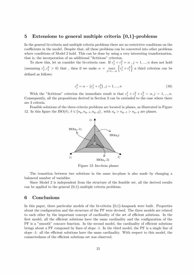
Feasible solutions of the three-criteria problems are located in planes, as illustrated in Figure12. In this …gure the ISO(±), ± 2fnq; nq¡1; nq¡2g ; with nq > nq¡1 > nq¡2 are planes.

ISO(nq)

ISO(nq -1)

ISO(nq -2) z2 z1

z3

Figure 12: Iso-item planes

The transition between two solutions in the same iso-plane is also made by changing abalanced number of variables.

Since Model 2 is independent from the structure of the feasible set, all the derived resultscan be applied to the general {0,1}-multiple criteria problems.

6 Conclusions

In this paper, three particular models of the bi-criteria {0,1}-knapsack were built. Propertiesabout the con…guration and the structure of the PF were devised. The three models are relatedto each other by the important concept of cardinality of the set of e¢cient solutions. In the…rst model, all the e¢cient solutions have the same cardinality and the con…guration of thePF is a ”smooth” concave function. In the second model, the cardinality of e¢cient solutionsbrings about a PF composed by lines of slope -1. In the third model, the PF is a single line ofslope -1: all the e¢cient solutions have the same cardinality. With respect to this model, theconnectedness of the e¢cient solutions set was observed.

21

Despite the restrictive formulations, in the previous section it was shown that general bi-criteria (and also multiple criteria) {0,1}-problems can be transformed in such a way that con-ditions of Model 2 hold.

Acknowledgements: The authors would like to acknowledge the support from MONETresearch project (POCTI/GES/37707/2001) and the third author also acknowledges the supportof the grant SFRH/BDP/6800/2001 (Fundação para a Ciência e Tecnologia, Portugal).

22

References

[1] Caprara, A., Kellerer, H., Pferschy, U., Pisinger, D. (2000) ”Approximation algorithmsfor knapsack problems with cardinality constraints”, European Journal of Operational Re-search, 123, pp. 333-345.

[2] Ehrgott, M., Klamroth, K. (1997) ”Connectedness of e¢cient solutions in multicriteriacombinatorial optimization”, European Journal of Operational Research, 97, pp. 159-166.

[3] Gomes da Silva, C., Figueira, J., Clímaco, J. (2003) ”An interactive procedure for thebi-criteria knapsack problems”, Research Report, No4, INESC-Coimbra, Portugal (in Por-tuguese). http://www.inescc.pt/download/RR2003_04.pdf

[4] Gomes da Silva, C., Clímaco, J., Figueira, J. (2004) ”A scatter search method for thebi-criteria knapsack problems”. To appear in European Journal of Operational Research.

[5] Isermann, H. (1977) ”The enumeration of the set of all e¢cient solutions for a linear mul-tiobjective programm”, Operational Research Quarterly, 28, 3, ii, pp. 711-725.

[6] Helbig, S. (1990) ”On the connectedness of the set of weakly e¢cient points of a vectoroptimization problem in locally convex spaces”, Journal of Optimization Theory and Ap-plications, 65, 2, pp. 257-270

[7] Murty, K. (1983) Linear Programming, John Wiley & Sons, Inc.

[8] Nemhauser, G., Wolsey, L. (1988) Integer Combinatorial Optimization, John Wiley & Sons,Inc.

[9] Pisinger, D. (1998) ”A fast algorithm for strongly correlated knapsack problems”, DiscreteApplied Mathematics, 89, pp. 197-212.

[10] Steuer, R. (1986) Multiple Criteria Optimization, Theory, Computation and Application,John Wiley & Sons, New York.

23

geometrical con…guration of the pareto frontier of … · geometrical con…guration of the...

Documents