geometry of diffeomorphism groups, … u = u(t,x) is a time-dependent vector ﬁeld on m satisfying...

Geom. Funct. Anal. Vol. 23 (2013) 334–366DOI: 10.1007/s00039-013-0210-2Published online March 7, 2013c© 2013 Springer Basel GAFA Geometric And Functional Analysis

GEOMETRY OF DIFFEOMORPHISM GROUPS, COMPLETEINTEGRABILITY AND GEOMETRIC STATISTICS

B. Khesin, J. Lenells, G. Misio�lek, and S. C. Preston

Abstract. We study the geometry of the space of densities Dens(M), which is thequotient space Diff(M)/Diffμ(M) of the diffeomorphism group of a compact man-ifold M by the subgroup of volume-preserving diffeomorphisms, endowed with aright-invariant homogeneous Sobolev H1-metric. We construct an explicit isometryfrom this space to (a subset of) an infinite-dimensional sphere and show that theassociated Euler–Arnold equation is a completely integrable system in any spacedimension whose smooth solutions break down in finite time. We also show that theH1-metric induces the Fisher–Rao metric on the space of probability distributionsand its Riemannian distance is the spherical version of the Hellinger distance.

Contents

1 Introduction . . . . . . . . . . . . . . . . . . . . . . . . . . . . . . . . . . . . . . . 3352 Geometric Background . . . . . . . . . . . . . . . . . . . . . . . . . . . . . . . . . 337

2.1 The Euler–Arnold equations. . . . . . . . . . . . . . . . . . . . . . . . . . . 3372.2 The optimal transport framework. . . . . . . . . . . . . . . . . . . . . . . . 339

3 The H1-Spherical Geometry of the Space of Densities . . . . . . . . . . . . . . . 3413.1 An infinite-dimensional sphere S∞

r . . . . . . . . . . . . . . . . . . . . . . . . 3413.2 The metric space structure of Diff(M)/Diffμ(M). . . . . . . . . . . . . . . . 3443.3 The Fisher–Rao metric in infinite dimensions. . . . . . . . . . . . . . . . . . 347

4 The Geodesic Equation: Solutions and Integrability . . . . . . . . . . . . . . . . . 3484.1 Local smooth solutions and explicit formulas. . . . . . . . . . . . . . . . . . 3494.2 Global properties of solutions. . . . . . . . . . . . . . . . . . . . . . . . . . . 3514.3 Complete integrability. . . . . . . . . . . . . . . . . . . . . . . . . . . . . . . 353

5 The Space of Metrics and the Diffeomorphism Group . . . . . . . . . . . . . . . . 3546 Applications and Discussion . . . . . . . . . . . . . . . . . . . . . . . . . . . . . . 357

6.1 Gradient flows. . . . . . . . . . . . . . . . . . . . . . . . . . . . . . . . . . . 3586.2 Shape theory. . . . . . . . . . . . . . . . . . . . . . . . . . . . . . . . . . . . 3596.3 Affine connections and duality. . . . . . . . . . . . . . . . . . . . . . . . . . 3596.4 The exponential map on Diff(M)/Diffμ(M). . . . . . . . . . . . . . . . . . . 361

Appendix A: The Euler–Arnold Equation of the a-b-c Metric . . . . . . . . . . . . . 362

Keywords and phrases: Diffeomorphism groups, Riemannian metrics, geodesics, curvature,Euler–Arnold equations, Fisher–Rao metric, Hellinger distance, integrable systems

Mathematics Subject Classification (2000): 53C21, 58D05, 58D17

GAFA GEOMETRY OF DIFFEOMORPHISM GROUPS 335

Acknowledgments . . . . . . . . . . . . . . . . . . . . . . . . . . . . . . . . . . . . . 365References . . . . . . . . . . . . . . . . . . . . . . . . . . . . . . . . . . . . . . . . . . 365

1 Introduction

The geometric approach to hydrodynamics pioneered by Arnold [Arn66] is basedon the observation that the particles of a fluid moving in a compact n-dimensionalRiemannian manifold M trace out a geodesic curve in the infinite-dimensional groupDiffμ(M) of volume-preserving diffeomorphisms (volumorphisms) of M . The generalframework of Arnold turned out to include a variety of nonlinear partial differentialequations of mathematical physics, now often referred to as Euler–Arnold equations.

Historically the metrics of most interest in infinite-dimensional Riemanniangeometry have been L2 metrics, which correspond to kinetic energy. On theother hand, in recent years there have appeared a number of interesting non-linear evolution equations described as geodesic equations on diffeomorphismgroups with respect to weak Riemannian metrics of Sobolev H1-type; see e.g.,[AK98,HMR98,KM03,You10] and their references. In this paper we focus on theH1 metrics both from a differential-geometric and a dynamical systems perspec-tive. Our main results concern the geometry of a subclass of such metrics, namely,degenerate right-invariant H1 Riemannian metrics on the full diffeomorphism groupDiff(M) and the properties of solutions of the associated geodesic equations. TheH1 metric is given at the identity diffeomorphism by

〈〈u, v〉〉 = b

∫

M

div u · div v dμ (1.1)

for some b > 0. It descends to a non-degenerate Riemannian metric on the homoge-neous space of right cosets (densities) Dens(M) = Diff(M)/Diffμ(M). Furthermore,it turns out that the corresponding geometry on densities is spherical for any compactmanifold M . More precisely, we prove that equipped with (1.1) the space Dens(M)is isometric to (a subset of) an infinite-dimensional sphere in a Hilbert space.

One motivation for studying this geometry is that such H1 metrics arise natu-rally on (generic) orbits of diffeomorphism groups in the manifold of all Riemannianstructures on M , using the natural Riemannian metric studied by Ebin [Ebi70]. Theinduced metric is a special case of the following general form of the right-invariant(a-b-c) Sobolev H1 metric on Diff(M) given at the identity by

〈〈u, v〉〉 = a

∫

M

〈u, v〉 dμ + b

∫

M

div u · div v dμ + c

∫

M

〈du�, dv�〉 dμ, (1.2)

where u, v ∈ TeDiff(M) are vector fields on M , μ is the Riemannian volume form,1 �is the isomorphism TM → T ∗M defined by the metric on M , and a, b and c are non-negative real numbers. We derive the Euler–Arnold equations for the metric (1.2) in

1 The volume form μ is denoted by dμ whenever it appears under the integral sign.

336 B. KHESIN ET AL. GAFA

the Appendix, which include as special cases the n-dimensional (inviscid) Burgersequation, the Camassa–Holm equation, as well as the Euler-α equation. A detailedstudy of the related curvatures appears in a separate publication [KLMP11].

In the special case of the homogeneous H1-metric (1.1) the Euler–Arnold equa-tion has the form

ρt + u · ∇ρ + 12ρ2 = −

∫M ρ2 dμ

2μ(M), (1.3)

where u = u(t, x) is a time-dependent vector field on M satisfying div u = ρ.2 Thisequation is a natural generalization of the completely integrable one-dimensionalHunter–Saxton equation [HS91] which is also known to yield geodesics on the homo-geneous space Diff(S1)/Rot(S1) (the quotient of the diffeomorphism group of thecircle by the subgroup of rotations), see [KM03].

We prove that the solutions of (1.3) describe the great circles on a sphere in aHilbert space, and, in particular, the equation is a completely integrable PDE forany number n of space variables. The corresponding complete family of conservedintegrals can be constructed in terms of angular momenta. Furthermore, we showthat the maximum existence time for smooth solutions of (1.3) is necessarily finitefor any initial conditions, with the L∞ norm of the solution growing without boundas t approaches the critical time. On the other hand, the geometry of the problempoints to a method of constructing global weak solutions.

The structure of the paper is as follows. In Section 2 we review the geomet-ric background on Euler–Arnold equations on Lie groups and describe the spaceof densities, as well as reductions to homogeneous spaces, particularly as relates toDiff(M), its subgroup Diffμ(M), and their quotient Dens(M).

In Section 3 we introduce the homogeneous H1-metric on the space of densitiesand study its geometry. Generalizing the results of [Len07] for the case of the circlewe show that for any n-dimensional manifold the space Dens(M) is isometric to asubset of the sphere in L2(M, dμ) with the induced metric. The H1 metric general-izes the Fisher–Rao information metric in geometric statistics and its Riemanniandistance is shown to be the spherical analogue of the Hellinger distance.

In Section 4 we study properties of solutions to the corresponding Euler–Arnoldequation. Since for M = S1 our equation reduces to the Hunter–Saxton equationwe thus obtain an integrable generalization of the latter to any space dimension.We show that all solutions break down in finite time and indicate how to constructglobal weak solutions. Finally we describe the construction of an infinite family ofconserved quantities.

In Section 5 we present a geometric approach which yields right-invariant metricsof the type (1.2) as induced metrics on the orbits of the diffeomorphism group fromthe canonical Riemannian L2 structures on the spaces of Riemannian metrics andvolume forms on the underlying manifold M .

2 We will show that the solution ρ does not depend on the choice of u, which happens preciselybecause the metric descends to the quotient space.


We conclude in Section 6 with some applications. First we discuss gradient flowon the space of densities in the spherical metric as a heat-like equation. Next wediscuss some applications to shape theory and compare with previous work, as wellas to the dual connections in geometric statistics. Finally we discuss Fredholmnessof the Riemannian exponential map. It also turns out that the H1-metric on thespace of densities described in this paper is isometric via the Calabi-Yau map to themetric on the space of Kahler metrics introduced in the 1950s by Calabi.3

In the Appendix we derive the Euler–Arnold equation for the general a-b-c met-ric (1.2) and show that several well-known PDE of mathematical physics can beobtained as special cases.

2 Geometric Background

2.1 The Euler–Arnold equations. In this section we describe the generalsetup which is convenient to study geodesics on Lie groups and homogeneous spacesequipped with right-invariant metrics.

Let G be a possibly infinite-dimensional Lie group with identity element e andTeG denoting the Lie algebra (we are primarily concerned with the case where Gis a subgroup of the group of C∞ diffeomorphisms of a compact manifold M with-out boundary, under the composition operation). We equip G with a right-invariant(possibly weak) Riemannian metric 〈〈·, ·〉〉 which is determined by its value at e. TheEuler–Arnold equation on the Lie algebra for the corresponding geodesic flow hasthe form

ut = −B(u, u) = −ad∗uu, (2.1)

where the bilinear operator B on TeG is defined by

〈〈B(u, v), w〉〉 = 〈〈u, advw〉〉, (2.2)

see [AK98] for details. In the case where G is a diffeomorphism group, the adjointoperation is given by advw = −[v, w], i.e., minus the Lie bracket of vector fields vand w on M .

Equation (2.1) describes the evolution in the Lie algebra of the vector u(t)obtained by right-translating the velocity along the geodesic η in G starting atthe identity with initial velocity u(0). The geodesic itself can be obtained by solvingthe Cauchy problem for the flow equation

dη

dt= Rη∗eu, η(0) = e.

3 We are grateful to B. Clarke and Y. Rubinstein for drawing our attention to this point, see moredetails in [CR11].


Example 2.1. Let G = Diffμ(M) be the group of volume-preserving diffeomor-phisms (volumorphisms) of a closed Riemannian manifold M . Consider the right-invariant metric on Diffμ(M) generated by the L2 inner product

〈〈u, v〉〉L2 =∫

M

〈u, v〉 dμ. (2.3)

In this case the Euler–Arnold equation (2.1) is the Euler equation of an ideal incom-pressible fluid in M

ut + ∇uu = −∇p, div u = 0, (2.4)

where u is the velocity field and p is the pressure function, see [Arn66]. In thevorticity formulation the 3D Euler equation becomes

ωt + [u, ω] = 0, where ω = curl u.

Example 2.2. Another source of examples are right-invariant Sobolev metrics onthe group G = Diff(S1) of circle diffeomorphisms; see e.g., [KM03]. Of particularinterest are those metrics whose Euler–Arnold equations turn out to be completelyintegrable. On Diff(S1) with the metric defined by the L2 product the Euler–Arnoldequation (2.1) becomes the (rescaled) inviscid Burgers equation

ut + 3uux = 0, (2.5)

while the H1 product yields the Camassa–Holm equation

ut − utxx + 3uux − 2uxuxx − uuxxx = 0. (2.6)

We also mention that if G is the Virasoro group, a one-dimensional central exten-sion of Diff(S1), equipped with the right-invariant L2 metric then the Euler–Arnoldequation is the periodic Korteweg-de Vries equation.

Now let H be a closed subgroup of G, and let G/H denote the homogeneousspace of right cosets. The following proposition characterizes those right-invariantRiemannian metrics on G which descend to a metric on G/H.

Proposition 2.3. A right-invariant metric 〈〈·, ·〉〉 on G descends to a right-invariantmetric on the homogeneous space G/H if and only if the inner product restricted toT⊥

e H (the orthogonal complement of TeH) is bi-invariant with respect to the actionby the subgroup H, i.e., for any u, v ∈ T⊥

e H ⊂ TeG and any w ∈ TeH one has

〈〈v, adwu〉〉 + 〈〈u, adwv〉〉 = 0. (2.7)

The proof repeats with minor changes the proof for the case of a metric that isdegenerate along a subgroup H; see [KM03].


Example 2.4. Let G = Diff(S1) and H = Rot(S1), with right-invariant metricgiven at the identity by

〈〈u, v〉〉H1 =∫

S1

uxvx dx.

The tangent space to the quotient Diff(S1)/Rot(S1) at the identity coset [e] can beidentified with the space of periodic functions of zero mean, and the correspondingEuler–Arnold equation is given by the Hunter–Saxton equation

utxx + 2uxuxx + uuxxx = 0, (2.8)

see [KM03]. In [Len07] the second author constructed an explicit isometry betweenthe quotient Diff(S1)/Rot(S1) and a subset of the unit sphere in L2(S1) anddescribed the corresponding solutions of equation (2.8) in terms of the geodesicflow on the infinite-dimensional sphere. Below we show that this observation is apart of a general phenomena valid for manifolds of any dimension.

2.2 The optimal transport framework. Given a volume form μ on M thereis a natural fibration of the diffeomorphism group Diff(M) over the space of vol-ume forms of fixed total volume μ(M) = 1. More precisely, the projection ontothe quotient space Diff(M)/Diffμ(M) defines a smooth ILH principal bundle4 withfibre Diffμ(M) and whose base is diffeomorphic to the space Dens(M) of normalizedsmooth positive densities (or, volume forms)

Dens(M) =

⎧⎨⎩ν ∈ Ωn(M) : ν > 0,

∫

M

dν = 1

⎫⎬⎭ ,

see Moser [Mos65]. Alternatively, let ρ = dν/dμ denote the Radon–Nikodym deriva-tive of ν with respect to the reference volume form μ. Then the base (as the space ofconstant-volume densities) can be regarded as a convex subset of the space of smoothpositive functions ρ on M normalized by the condition

∫M ρ dμ = 1. In this case

the projection map π can be written explicitly as π(η) = Jacμ(η−1) where Jacμ(η)denotes the Jacobian of η computed with respect to μ, that is, η∗μ = Jacμ(η)μ.The projection π satisfies π(η ◦ ξ) = π(η) whenever ξ ∈ Diffμ(M), i.e., wheneverJacμ(ξ) = 1. Thus π is constant on the left cosets and descends to an isomorphismbetween the quotient space of left cosets to the space of densities.

The group Diff(M) carries a natural L2-metric

〈〈u ◦ η, v ◦ η〉〉L2 =∫

M

〈u ◦ η, v ◦ η〉 dμ =∫

M

〈u, v〉Jacμ(η−1) dμ (2.9)

4 In the Sobolev category Diffs(M) → Diffs(M)/Diffsμ(M) is a C0 principal bundle for any suffi-

ciently large s > n/2 + 1, see [EM70].


Table 1 The geometric structures associated with L2 and H1 optimal transport

Diff(M) Diffμ(M) Dens(M) = Diff(M)/Diffμ(M)

L2-metric(non-invariant)

L2-right invariant metric(ideal hydrodynamics)

Wasserstein distance(L2-optimal transport)

H1-metric(right-invariant)

Degenerate (identicallyvanishing)

Spherical Hellinger distance(H1-optimal transport)

where u, v ∈ TeDiff(M) and η ∈ Diff(M). This metric is neither left- nor right-invari-ant, although it becomes right-invariant when restricted to the subgroup Diffμ(M)of volumorphisms and becomes left-invariant only on the subgroup of isometries.Following Otto [Ott01] one can then introduce a metric on the base Dens(M) forwhich the projection π is a Riemannian submersion: vertical vectors at TηDiff(M)are those fields u ◦ η with div (ρu) = 0, and horizontal fields are of the form ∇f ◦ ηfor some f : M → R, since the differential of the projection is π∗(v ◦ η) = − div (ρv)where ρ = π(η).5

The associated Riemannian distance in Diff(M)/Diffμ(M) between two measuresν and λ has an elegant interpretation as the L2-cost of transporting one density tothe other

dist2W (ν, λ) = infη

∫

M

dist2M (x, η(x)) dμ (2.10)

with the infimum taken over all diffeomorphisms η such that η∗λ = ν and wheredistM denotes the Riemannian distance on M ; see [BB01] or [Ott01]. The functiondistW is called the L2-Wasserstein (or Kantorovich-Rubinstein) distance between μand ν in optimal transport theory.

Remark 2.5. While the non-invariant L2 metric (2.9) on Diff(M) descends to Otto’smetric on the quotient space Dens(M) = Diff(M)/Diffμ(M), one verifies that amongnon-invariant H1 metrics of this type it is the only one descending to the quotientDens(M).

The situation is different for invariant metrics. Recall that the general conditionfor a right-invariant metric on a group G to descend to the quotient G/H withrespect to a closed subgroup H was given in Proposition 2.3. Note that this con-dition is precisely what one needs in order for the projection map from G to G/Hto be a Riemannian submersion, i.e., that the length of every horizontal vector ispreserved under the projection.

It turns out that the degenerate right-invariant H1 metric (1.1) on Diff(M)descends to a non-degenerate metric on Dens(M). The skew symmetry condition(2.7) in this case will be verified in Theorem 4.1. On the other hand, one can check

5 The construction in [Ott01] actually comes from Jacμ(η−1), which is important since it is left-invariant, not right-invariant.


that the right-invariant L2-metric (2.3) does not verify (2.7) and hence does notdescend. Similarly, the full H1 metric on Diff(M) obtained by right-translating thea-b-c product (1.2) also fails to descend to a metric on Dens(M). This is summarizedin Table 1.

3 The H1-Spherical Geometry of the Space of Densities

In this section we study the homogeneous space of densities Dens(M) on a closedn-dimensional Riemannian manifold M equipped with the right-invariant metricinduced by the H1 inner product (1.1), that is

〈〈u ◦ η, v ◦ η〉〉H1 =14

∫

M

div u · div v dμ (3.1)

for any u, v ∈ TeDiff(M) and η ∈ Diff(M). It corresponds to the a = c = 0 term inthe general (a-b-c) Sobolev H1 metric (1.2) of the Introduction in which, to simplifycalculations, we set b = 1/4. (We will return to the case of any b > 0 in Section 5and Appendix A.)

The geometry of this metric on the space of densities turns out to be particularlyremarkable. Indeed, we prove below that Dens(M) endowed with the metric (3.1) isisometric to a subset of a round sphere in the space of square-integrable functions onM .6 Moreover, we show that (3.1) corresponds to the Bhattacharyya coefficient (alsocalled the affinity) in probability and statistics and that it gives rise to a sphericalvariant of the Hellinger distance. Thus the right-invariant H1-metric provides goodalternative notions of distance and shortest path for (smooth) probability measureson M to the ones obtained from the L2-Wasserstein constructions used in standardoptimal transport problems.

3.1 An infinite-dimensional sphere S∞r . We begin by constructing an isom-

etry between the homogeneous space of densities Dens(M) and a subset of the sphereof radius r

S∞r =

⎧⎨⎩f ∈ L2(M, dμ) :

∫

M

f2 dμ = r2

⎫⎬⎭

in the Hilbert space L2(M, dμ). As before, we let Jacμ(η) be the Jacobian of η withrespect to μ and let μ(M) stand for the total volume of M .

Theorem 3.1. The map Φ : Diff(M) → L2(M, dμ) given by

Φ : η → f =√

Jacμη

6 This construction has an antecedent in the special case of the group of circle diffeomorphismsconsidered in [Len07].


defines an isometry from the space of densities Dens(M) = Diff(M)/Diffμ(M)equipped with the H1-metric (3.1) to a subset of the sphere S∞

r ⊂ L2(M, dμ) ofradius

r =√

μ(M)

with the standard L2 metric.For s > n/2 + 1 the map Φ is a diffeomorphism between Diffs(M)/Diffs

μ(M) andthe convex open subset of S∞

r ∩Hs−1(M) which consists of strictly positive functionson M .

Proof. First, observe that the Jacobian of any orientation-preserving diffeomorphismis a strictly positive function. Next, using the change of variables formula, we findthat ∫

M

Φ2(η) dμ =∫

M

Jacμη dμ =∫

M

η∗ dμ =∫

η(M)

dμ = μ(M)

which shows that Φ maps diffeomorphisms into S∞r . Furthermore, observe that since

for any ξ ∈ Diffμ(M) we have

Jacμ(ξ ◦ η)μ = (ξ ◦ η)∗μ = η∗μ = Jacμ(η)μ;

it follows that Φ is well-defined as a map from Diff(M)/Diffμ(M).Next, suppose that for some diffeomorphisms η1 and η2 we have Jacμ(η1) =

Jacμ(η2). Then (η1 ◦ η−12 )∗μ = μ from which we deduce that Φ is injective. More-

over, differentiating the formula Jacμ(η)μ = η∗μ with respect to η and evaluatingat U ∈ TηDiff(M), we obtain

Jacμ∗η(U) = div(U ◦ η−1) ◦ η Jacμη.

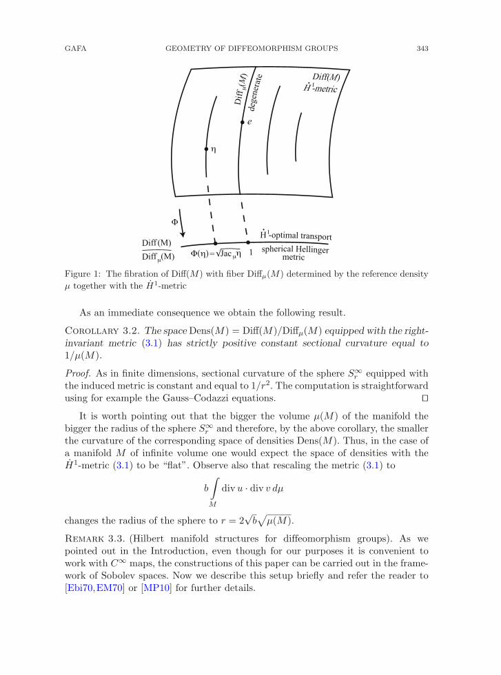
Therefore, letting π : Diff(M) → Diff(M)/Diffμ(M) denote the bundle projection,see Figure 1, we find that

〈〈(Φ ◦ π)∗η(U), (Φ ◦ π)∗η(V )〉〉L2 =14

∫

M

(div u ◦ η) · (div v ◦ η) Jacμη dμ

=14

∫

M

div u · div v dμ = 〈〈U, V 〉〉H1 ,

for any elements U = u ◦ η and V = v ◦ η in TηDiff(M) where η ∈ Diff(M). Thisshows that Φ is an isometry.

When s > n/2 + 1 the above arguments extend to the category of Hilbert man-ifolds modelled on Sobolev Hs spaces, see Remark 3.3 below. The fact that anypositive function in S∞

r ∩ Hs−1(M) belongs to the image of the map Φ follows fromMoser’s Lemma [Mos65] whose generalization to the Sobolev setting can be foundfor example in [EM70]. ��


1

Figure 1: The fibration of Diff(M) with fiber Diffμ(M) determined by the reference densityμ together with the H1-metric

As an immediate consequence we obtain the following result.

Corollary 3.2. The space Dens(M) = Diff(M)/Diffμ(M) equipped with the right-invariant metric (3.1) has strictly positive constant sectional curvature equal to1/μ(M).

Proof. As in finite dimensions, sectional curvature of the sphere S∞r equipped with

the induced metric is constant and equal to 1/r2. The computation is straightforwardusing for example the Gauss–Codazzi equations. ��

It is worth pointing out that the bigger the volume μ(M) of the manifold thebigger the radius of the sphere S∞

r and therefore, by the above corollary, the smallerthe curvature of the corresponding space of densities Dens(M). Thus, in the case ofa manifold M of infinite volume one would expect the space of densities with theH1-metric (3.1) to be “flat”. Observe also that rescaling the metric (3.1) to

b

∫

M

div u · div v dμ

changes the radius of the sphere to r = 2√

b√

μ(M).

Remark 3.3. (Hilbert manifold structures for diffeomorphism groups). As wepointed out in the Introduction, even though for our purposes it is convenient towork with C∞ maps, the constructions of this paper can be carried out in the frame-work of Sobolev spaces. Now we describe this setup briefly and refer the reader to[Ebi70,EM70] or [MP10] for further details.


For a compact Riemannian manifold M , the set Hs(M, M) consists of mapsf : M → M such that for any p ∈ M and for any local chart (U, φ) at p and anylocal chart (V, φ) at f(p), the composition φ◦f ◦φ−1 belongs to Hs(φ(U), Rn). Usingthe Sobolev Lemma, one shows that if s > n/2, then this definition is independentof the choice of charts on M . The tangent space at f ∈ Hs(M, M) is defined asthe set of all Hs-sections of the pull-back bundle TfHs(M, M) = Hs(f−1TM). Adifferentiable atlas for Hs(M, M) is constructed using the Riemannian exponen-tial map on M . For example, to find a chart at the identity map f = e considerExp : TM → M ×M given by Exp(v) =

(π(v), expπ(v) vπ(v)

)where π : TM → M is

the tangent bundle projection. Since Exp is a diffeomorphism from an open subset Ucontaining the zero section in TM onto a neighbourhood of the diagonal in M ×M ,one can define a bijection from the set

Ue = {v ∈ Hs(TM) : v(M) ⊂ U}onto a neighbourhood of the identity map in Hs(M, M) by

Φ : Ue ⊂ TeHs(M, M) → Hs(M, M), v → Φ(v) = Exp ◦ v.

The pair (Ue, Φ) gives a chart in Hs(M, M) around f = e. Compactness, prop-erties of exp and standard facts about compositions of Sobolev maps ensure thatthe charts are well-defined and independent of the Riemannian metric on M , withsmooth transition functions on the overlaps.

For any s > n/2 + 1 the group of Hs diffeomorphisms can be now defined as

Diffs(M) = C1Diff(M) ∩ Hs(M, M),

where C1Diff(M) is the set of C1 diffeomorphisms of M . Since C1Diff(M) formsan open set in C1(M, M), it follows by the Sobolev Lemma that Diffs(M) is alsoopen as a subset of the Hilbert manifold Hs(M, M) and hence itself a smooth man-ifold. Furthermore, it is a topological group under composition of diffeomorphisms.In fact, right multiplications Rη(ξ) = ξ ◦ η are smooth in the Hs topology, whereasleft multiplications Lη(ξ) = η ◦ ξ and inversions η → η−1 are continuous but notLipschitz continuous. The subgroup of volume-preserving diffeomorphisms

Diffsμ(M) = {η ∈ Diff(M) : η∗μ = μ}

is a closed C∞ submanifold of Diffs(M). This follows essentially from the implicitfunction theorem for Banach manifolds and the Hodge decomposition.

3.2 The metric space structure of Diff(M)/Diffµ(M). The right invari-ant metric (3.1) induces a distance function between densities (measures) of fixedtotal volume on M that is analogous to the Wasserstein distance (2.10) induced bythe non-invariant L2 metric used in the standard optimal transport. It turns out thatthe isometry Φ constructed in Theorem 3.1 makes the computations of distances inDens(M) with respect to (3.1) simpler than one would expect by comparison withthe Wasserstein case.


Consider two (smooth) measures λ and ν on M of the same total volume μ(M)which are absolutely continuous with respect to the reference measure μ. Let dλ/dμand dν/dμ be the corresponding Radon–Nikodym derivatives of λ and ν with respectto μ.

Theorem 3.4. The Riemannian distance defined by the H1-metric (3.1) betweenmeasures λ and ν in the density space Dens(M) = Diff(M)/Diffμ(M) is

distH1(λ, ν) =√

μ(M) arccos

⎛⎝ 1

μ(M)

∫

M

√dλ

dμ

dν

dμdμ

⎞⎠. (3.2)

Equivalently, if η and ζ are two diffeomorphisms mapping the volume form μ toλ and ν, respectively, then the H1-distance between η and ζ is

distH1(η, ζ) = distH1(λ, ν) =√

μ(M) arccos

⎛⎝ 1

μ(M)

∫

M

√Jacμη · Jacμζ dμ

⎞⎠ .

Proof. Let f2 = dλ/dμ and g2 = dν/dμ. If λ = η∗μ and ν = ζ∗μ then using theexplicit isometry Φ constructed in Theorem 3.1 it is sufficient to compute the dis-tance between the functions Φ(η) = f and Φ(ζ) = g considered as points on thesphere S∞

r with the induced metric from L2(M, dμ). Since geodesics of this metricare the great circles on S∞

r it follows that the length of the corresponding arc joiningf and g is given by

r arccos

⎛⎝ 1

r2

∫

M

fg dμ

⎞⎠,

which is precisely formula (3.2). ��We can now compute precisely the diameter of the space of densities using stan-

dard formula

diamH1 Dens(M) := sup{

distH1(λ, ν) : λ, ν ∈ Dens(M)}.

Corollary 3.5. The diameter of the space Dens(M) equipped with the H1-metric(3.1) equals π

2

√μ(M), or one quarter the circumference of S∞

r .

Proof. The upper bound follows easily from formula (3.2), since the argument ofthe arccosine is always between 0 and 1. To prove it is arbitrarily close to 0, wechoose the positive functions f and g as in the proof of Theorem 3.4 with supportsconcentrated in disjoint areas. ��

The Riemannian distance function distH1 on the space of densities Dens(M)introduced in Theorem 3.4 is very closely related to the Hellinger distance in proba-bility and statistics. Recall that given two probability measures λ and ν on M that


are absolutely continuous with respect to a reference probability μ the Hellingerdistance between λ and ν is defined as

dist2Hel(λ, ν) =∫

M

(√dλ

dμ−√

dν

dμ

)2

dμ.

As in the case of distH1 one checks that distHel(λ, ν) =√

2 when λ and ν are mutu-ally singular and that distH(λ, ν) = 0 when the two measures coincide. It can alsobe expressed by the formula dist2Hel(λ, ν) = 2 (1 − BC(λ, ν)) , where BC(λ, ν) is theso-called Bhattacharyya coefficient (affinity) used to measure the “overlap” betweenstatistical samples; see e.g., [Che82] for more details.

In order to compare the Hellinger distance distHel with the Riemannian distancedistH1 defined in (3.2) recall that probability measures λ and ν are normalized bythe condition λ(M) = ν(M) = μ(M) = 1. As before, we shall consider the squareroots of the respective Radon–Nikodym derivatives as points on the (unit) spherein L2(M, dμ). One can immediately verify the following two corollaries of Theorem3.1.

Corollary 3.6. The Hellinger distance distHel(λ, ν) between the normalized den-sities dλ = f2dμ and dν = g2dμ is equal to the distance in L2(M, dμ) between thepoints on the unit sphere f, g ∈ S∞

1 ⊂ L2(M, dμ).

Corollary 3.7. The Bhattacharyya coefficient BC(λ, ν) for two normalized den-sities dλ = f2dμ and dν = g2dλ is equal to the inner product of the correspondingpositive functions f and g in L2(M, dμ):

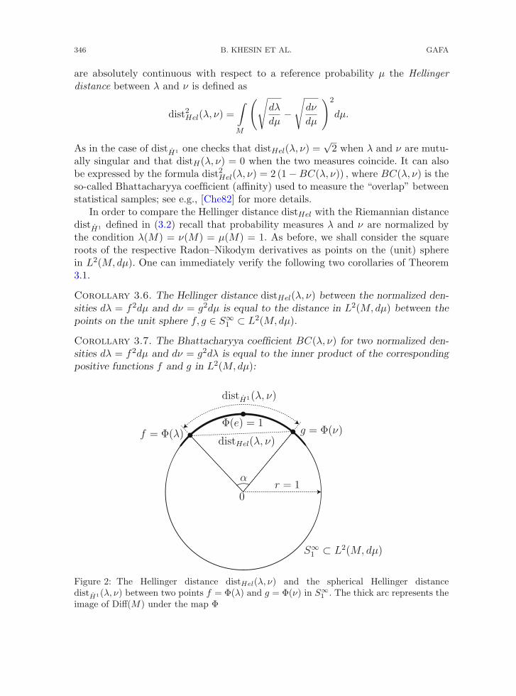
Figure 2: The Hellinger distance distHel(λ, ν) and the spherical Hellinger distancedistH1(λ, ν) between two points f = Φ(λ) and g = Φ(ν) in S∞

1 . The thick arc represents theimage of Diff(M) under the map Φ


BC(λ, ν) =∫

M

√dλ

dμ

dν

dμdμ =

∫

M

fg dμ.

Let 0 < α < π/2 denote the angle between f and g viewed as unit vectors inL2(M, dμ). Then we have

distHel(λ, ν) = 2 sin(α/2) and BC(λ, ν) = cos α,

while

distH1(λ, ν) = α = arccos BC(λ, ν).

Thus, we can refer to the Riemannian distance distH1(λ, ν) on Dens(M) as thespherical Hellinger distance between λ and ν, see Figure 2.

3.3 The Fisher–Rao metric in infinite dimensions. It is remarkable thatthe right-invariant H1 metric (3.1) provides an appropriate geometric frameworkfor an infinite-dimensional Riemannian approach to mathematical statistics. Effortsdirected toward finding suitable differential geometric approaches to statistics goback to the work of Fisher, Rao [Rao93] and Kolmogorov.

In the classical approach one considers finite-dimensional families of probabilitydistributions on M whose elements are parameterized by subsets E of the Euclideanspace R

k,

S ={

ν = νs1,...,sk∈ Dens(M) : (s1, . . . , sk) ∈ E ⊂ R

k}

.

When equipped with a structure of a smooth k-dimensional manifold such a familyis referred to as a statistical model. Rao [Rao93] showed that any S carries a naturalstructure given by a k × k positive definite matrix

Iij =∫

M

∂ log ν

∂si

∂ log ν

∂sjν dμ (i, j = 1, . . . , k), (3.3)

called the Fisher–Rao (information) metric.7

In our approach we shall regard a statistical model S as a k-dimensional Rie-mannian submanifold of the infinite-dimensional Riemannian manifold of probabil-ity densities Dens(M) defined on the underlying n-dimensional compact manifold M .The following theorem shows that the Fisher–Rao metric (3.3) is (up to a constantmultiple) the metric induced on the submanifold S ⊂ Dens(M) by the (degenerate)right-invariant Sobolev H1-metric (1.1) we introduced originally on the full diffeo-morphism group Diff(M).

7 The significance of this metric for statistics was also noted by Chentsov [Che82]. An infinite-dimensional version was perhaps first mentioned by Dawid in a commentary [Daw77] on the paperof Efron [Efr75].


Theorem 3.8. The right-invariant Sobolev H1-metric (3.1) on the quotient spaceDens(M) of probability densities on M coincides with the Fisher–Rao metric on anyk-dimensional statistical submanifold of Dens(M).

Proof. We carry out the calculations directly in Diff(M). Given any v and w inTeDiff(M), consider a two-parameter family of diffeomorphisms (s1, s2) → η(s1, s2)in Diff(M) starting from the identity η(0, 0) = e with ∂

∂s1η(0, 0) = v, ∂

∂s2η(0, 0) = w.

Let

v(s1, s2) ◦ η(s1, s2) = ∂∂s1

η(s1, s2) and w(s1, s2) ◦ η(s1, s2) = ∂∂s2

η(s1, s2)

be the corresponding variation vector fields along η(t, s).If ρ is the Jacobian of η(s1, s2) computed with respect to the fixed measure μ,

then (3.3) takes the form

Ivw =∫

M

∂

∂s1(log Jacμη(s1, s2))

∂

∂s2(log Jacμη(s1, s2)) Jacμη(s1, s2) dμ.

Recall that∂

∂s1Jacμη(s1, s2) = div v(s1, s2) ◦ η(s1, s2) · Jacμη(s1, s2)

and similarly for the partial derivative in s2. Using these formulas and changingvariables in the integral, we now find

Ivw =∫

M

∂∂s1

Jacμη(s1, s2) ∂∂s2

Jacμη(s1, s2)Jacμη(s1, s2)

∣∣s1=s2=0

dμ

=∫

M

(div v ◦ η

) · (div w ◦ η)

Jacμη dμ

=∫

M

div v · div w dμ = 4〈〈v, w〉〉H1 ,

from which the theorem follows. ��Theorem 3.8 suggests that the H1 counterpart of optimal transport with its asso-

ciated spherical Hellinger distance is the infinite-dimensional version of geometricstatistics sought in [AN00] and [Che82].

4 The Geodesic Equation: Solutions and Integrability

In the preceding sections we studied the geometry of the H1-metric (3.1) on thespace of densities Dens(M). In this section we shall focus on obtaining explicit for-mulas for solutions of the Cauchy problem for the associated Euler–Arnold equationand prove that they necessarily break down in finite time.


4.1 Local smooth solutions and explicit formulas. First we derive the geo-desic equation induced on the quotient Dens(M) by the Riemannian metric (1.1).

Theorem 4.1. If a = c = 0 then the a-b-c metric (1.2) satisfies condition (2.7) andtherefore descends to a metric on the space of densities Dens(M). The correspondingEuler–Arnold equation is

∇ div ut + div u ∇ div u + ∇〈u, ∇ div u〉 = 0 (4.1)

or, in the integrated form,

ρt + 〈u, ∇ρ〉 + 12ρ2 = −

∫M ρ2 dμ

2μ(M)(4.2)

where ρ = div u.

Proof. We verify (2.7) for G = Diff(M), H = Diffμ(M) and adwv = −[w, v], where[·, ·] is the Lie bracket of vector fields on M . Given any vector fields u, v and w withdiv w = 0, we have

〈〈adwv, u〉〉H1 + 〈〈v, adwu〉〉H1 = −b

∫

M

(div [w, v] div u + div [w, u] div v

)dμ

= −b

∫

M

((〈w, ∇ div v〉 − 〈v,∇ div w〉)div u

+(〈w, ∇ div u〉 − 〈u, ∇ div w〉) div v

)dμ

= b

∫

M

div w · div v · div u dμ = 0,

which shows that (1.2) descends to Diff(M)/Diffμ(M).The Euler–Arnold equation on the quotient can be now obtained from

(A.4) in the form (4.1). In integrated form it reads

div ut + 〈u, div u〉 + 12(div u)2 = C(t)

where C(t) may in general depend on time. Integrating this equation over M deter-mines the value of C(t). ��

Note that in the special case M = S1 differentiating equation (4.2) with respectto the space variable gives the Hunter–Saxton equation (2.8). The gradient of (4.2),augmented by terms arising from an additional L2 term in (1.1), was derived as a2D water wave equation in [KSD01], thus our equation represents a limiting case.

Remark 4.2. The right-hand side of equation (4.2) is independent of time for anyinitial condition ρ0 because the integral

∫M ρ2 dμ corresponds to the energy (the

squared length of the velocity) in the H1-metric on Dens(M) and is constant alonga geodesic. This invariance will also be verified by a direct computation in the proofbelow.


Consider an initial condition in the form

ρ(0, x) = div u0(x). (4.3)

We already have an indirect method for solving the initial value problem for equa-tion (4.2) by means of Theorem 3.1. We now proceed to give explicit formulas forthe corresponding solutions.

Theorem 4.3. Let ρ = ρ(t, x) be the solution of the Cauchy problem (4.2)–(4.3)and suppose that t → η(t) is the flow of the velocity field u = u(t, x), i.e., ∂

∂tη(t, x) =u(t, η(t, x)) where η(0, x) = x. Then

ρ(t, η(t, x)

)= 2κ tan

(arctan

div u0(x)2κ

− κt

), (4.4)

where

κ2 =1

4μ(M)

∫

M

(div u0)2 dμ. (4.5)

Furthermore, the Jacobian of the flow is

Jacμ

(η(t, x)

)=(

cos κt +div u0(x)

2κsin κt

)2. (4.6)

Proof. For any smooth real-valued function f(t, x) the chain rule gives

d

dt(f(t, η(t, x))) =

∂f

∂t(t, η(t, x)) + 〈u (t, η(t, x)) , ∇f (t, η(t, x))〉 .

Using this we obtain from (4.2) an equation for f = ρ ◦ η

df

dt+ 1

2f2 = −C(t), (4.7)

where C(t) = (2μ(M))−1∫M ρ2dμ, as remarked above, is in fact independent of time.

Indeed, direct verification gives

μ(M)dC(t)

dt=∫

M

ρρt dμ =∫

M

div u div ut dμ

= −∫

M

〈u, ∇ div u〉 div u dμ − 12

∫

M

(div u)3 dμ = 0,

where the last cancellation follows from integration by parts.Set C = 2κ2. Then, for a fixed x ∈ M the solution of the resulting ODE in (4.7)

with initial condition f(0) has the form

f(t) = 2κ tan (arctan (f(0)/2κ) − κt) ,


which is precisely (4.4).In order to find an explicit formula for the Jacobian we first compute the time

derivative of Jacμ(η)μ to obtain

d

dt(Jacμ(η)μ) =

d

dt(η∗μ) = η∗(Luμ) = η∗(div u μ) = (ρ ◦ η) Jacμ(η)μ.

This gives a differential equation for Jacμη, which we can now solve with the helpof (4.4) to get the solution in the form of (4.6). ��

Note that (4.6) completely determines the Jacobian regardless of any “ambi-guity” in the velocity field u satisfying div u = ρ in equation (4.2). The reason isthat the Jacobians can be considered as elements of the quotient space Dens(M) =Diff(M)/Diffμ(M) (a convenient way to resolve the ambiguity is by choosing velocityas the gradient field u = ∇Δ−1ρ).

Remark 4.4 (Great circles on S∞r ). We emphasize that formula (4.6) for the Jaco-

bian Jacμη of the flow is best understood in light of the correspondence betweengeodesics in Dens(M) and those on the infinite-dimensional sphere S∞

r establishedin Theorem 3.1. Indeed, the map

t →√

Jacμ (η(t, x)) = cos κt +div u0(x)

2κsin κt

describes the great circle on the unit sphere S∞1 ⊂ L2(M, dμ) passing through the

point 1 with initial velocity 12 div u0.

4.2 Global properties of solutions. The explicit formulas of Theorem 4.3make it possible to give a fairly complete picture of the global behavior of solutionsto the H1 Euler–Arnold equation on Dens(M) for any manifold M . It turns outfor example that any smooth solution of equation (4.2) has finite lifespan and theblowup mechanism can be precisely described.

By the result of Moser [Mos65], the function on the right side of formula (4.6)will be the Jacobian of some diffeomorphism as long as it is nowhere zero. Henceup to the blowup time we have a smooth path in the space of densities, which liftsto a smooth path in the diffeomorphism group; see Proposition 4.6. Geodesics leavethe set of positive densities and hit the boundary corresponding to the boundaryof the diffeomorphism group. The latter consists of Hs maps from M to M , whichare degenerations of diffeomorphisms. To make sense of weak solutions of (4.2), onewould need a way of lifting the curve (4.6) to a smooth curve in Hs(M, M).

First, we note that there can be no global smooth (classical) solutions of theEuler–Arnold equation (4.2). As in the case of the one-dimensional Hunter–Saxtonequation all solutions break down in finite time.

Proposition 4.5. The maximal existence time of a (smooth) solution of the Cauchyproblem (4.2)–(4.3) constructed in Theorem 4.3 is

0 < Tmax =π

2κ+

1κ

arctan(

12κ

infx∈M

div u0(x))

. (4.8)


Furthermore, as t ↗ Tmax we have ‖u(t)‖C1 ↗ ∞.

Proof. This follows at once from formula (4.4) using the fact that div u = ρ. Alter-natively, from formula (4.6) we observe that the flow of u(t, x) ceases to be a diffe-omorphism at t = Tmax. ��

Observe that before a solution reaches the blow-up time it is always possible tolift the corresponding geodesic to a smooth flow of diffeomorphisms using a slightvariation of the classical construction of Moser [Mos65].

Proposition 4.6. If div u0 is smooth, then there exists a family of smooth diffeo-morphisms η(t) in Diff(M) satisfying (4.6), i.e., such that Jacμ(η(t)) = ϕ(t) where

ϕ(t, x) =(

cos κt +div u0(x)

2κsin κt

)2

, (4.9)

provided that 0 ≤ t < Tmax. Furthermore η is smooth in time as a curve in Diff(M).If u0 is in Hs for s > n/2 + 1, the curve η(t) is in Diffs(M).

Proof. It is easy to check that∫M ϕ(t, x) dμ is constant in time, which allows one

to solve the equation Δf(t, x) = −∂ϕ/∂t(t, x) for f , for any fixed time t. Using theexplicit formula (4.9), we easily see that f is smooth in time and spatially in Hs+1

if u0 is in Hs.For t in [0, Tmax), we define a time-dependent vector field by the formula X(t, x) =

∇f(t, x)/ϕ(t, x). Let t → ξ(t) denote the flow of X starting at the identity (whichexists for t ∈ [0, Tmax) and x ∈ M by compactness of M). Using the definition of fand LX(ϕμ) = div (ϕX)μ, we compute

d

dtξ∗(ϕμ) = ξ∗

(∂ϕ

∂tμ + LX(ϕμ)

)= 0.

Since ϕ(0) = 1 and ξ(0) = e we have ξ∗(ϕμ) = μ for any 0 ≤ t < Tmax. Denotingby η(t) the inverse of the diffeomorphism ξ(t), we find that η∗μ = ϕμ, from whichit follows that Jacμ(η(t, x)) = ϕ(t, x) as desired. ��

The method of Proposition 4.6 gives a particular choice of a diffeomorphism flowη, and hence a velocity field appearing in (4.2) and satisfying div u = ϕ. The flowmust break down at the critical time Tmax, since the vector field X becomes singular(when ϕ reaches zero). The difficulty here is that one constructs η indirectly, by firstconstructing ξ = η−1, and it is this inversion procedure that breaks down at theblowup time Tmax.

For the Hunter–Saxton equation on Diff(S1)/Rot(S1) the related construction ofweak solutions was explained in [Lene07]. In this case the flow is determined (up torotations of the base point) by its Jacobian. If the initial velocity is not constant inany interval, then the singularities of the flow are isolated so that it is a homeomor-phism (but not a diffeomorphism past the blowup time). In terms of the spherical


picture, the square root map Φ from Theorem 3.1 maps only onto a small portionof the space of functions with fixed L2 norm, but its inverse can be defined on theentire sphere. In higher dimensions if the Jacobian is not everywhere positive thesituation is much more complicated. Nevertheless, in this case it may be possible toapply the techniques of Gromov and Eliashberg [GE73] in order to construct a mapwith a prescribed Jacobian. It would be interesting to extend Moser’s argument toconstruct a global flow of homeomorphisms out of this flow of maps (past the blowuptime).

4.3 Complete integrability. For a 2n-dimensional Hamiltonian system, com-plete integrability means the existence of n functionally independent integralsH1, . . . , Hn in involution (one of which is the Hamiltonian of the system); in sucha case the motion can be determined by quadrature. In infinite dimensions the sit-uation is more subtle: the existence of infinitely many constants of motion maynot suffice to determine the motion. Infinite-dimensional systems have been studiedintensively since the discovery of the complete integrability of the Korteweg-de Vriesequation. Other examples include one-dimensional equations like the Camassa–Holmand Hunter–Saxton equations, and two-dimensional examples like the Kadomtsev–Petviashvili, Ishimori, and Davey–Stewartson equations.

In addition to having an explicit formula for solutions (see Theorem 4.3), onecan also construct infinitely many independent constants of motion, using the factthat geodesic motion on a sphere of any dimension is completely integrable. Firstconsider the unit sphere Sn−1 ⊂ R

n, given by the equation∑n

j=1 q2j = 1 with

q = (q1, . . . , qn) ∈ Rn and equipped with its standard round metric. The geodesic

flow in this metric is defined by the Hamiltonian H =∑n

j=1 p2j on the cotangent

bundle T ∗Sn−1. It is a classical example of a completely integrable system, whichhas the property that all of its orbits are closed.

Proposition 4.7. (see e.g., [Bol10])

(i) The functions hij = piqj − pjqi, 1 ≤ i < j ≤ n on T ∗R

n (as well as theirreductions to T ∗Sn−1) commute with the Hamiltonian H =

∑nj=1 p2

j andgenerate the Lie algebra so(n).

(ii) The functions

Hk :=∑

1≤i<j≤k

h2ij =

k∑j=1

p2j

k∑j=1

q2j −

⎛⎝ k∑

j=1

qjpj

⎞⎠

2

for k = 2, . . . , n form a complete set of independent integrals in involutionfor the geodesic flow on the round sphere Sn−1 ⊂ R

n, that is {Hi, Hj} = 0,for any 2 ≤ i, j ≤ n.

Proof. The Hamiltonian functions hij in T ∗R

n generate rotations in the (qi, qj)-planein R

n, which are isometries of Sn−1. These rotations commute with the geodesic flow


on the sphere and hence {hij , H} = 0. A direct computation gives {hij , hjk} = hik,which are the commutation relations of so(n).

The involutivity of Hk is a routine calculation. ��Alternatively, one can consider the chain of subalgebras so(2) ⊂ so(3) ⊂ · · · ⊂

so(n). Then Hk is one of the Casimir functions for so(k) and it therefore commuteswith any function on so(k)∗. In particular, it commutes with all the preceding func-tions Hm for m < k. They are functionally independent because at each step Hk

involves new functions hjk. Note that on the cotangent bundle T ∗Sn−1 the functionHn coincides with the Hamiltonian H since

∑nj=1 q2

j = 1 and∑n

j=1 piqi = 0 (“thetangent plane equation”).

The same procedure allows one to construct integrals in infinite dimensions, forS∞

r ⊂ L2(M, dμ). Similarly, on the cotangent space T ∗S∞r with position coordinates

qi and momentum coordinates pi, Hamiltonians hij = piqj − pjqi generate rotationsof the sphere in the (qi, qj)-plane. They now form the Lie algebra so(∞) of thegroup of unitary operators on L2 and generate an infinite sequence of functionallyindependent first integrals {Hk}∞

k=2 in involution. This sequence corresponds to theinfinite chain of embeddings so(2) ⊂ so(3) ⊂ · · · ⊂ so(∞) and provides infinitelymany conserved quantities for the geodesic flow on the unit sphere S∞

r ⊂ L2(M, dμ).We summarize the above consideration in the following

Theorem 4.8. The Euler–Arnold equation (4.2) of the right-invariant H1-metricon the space of densities Dens(M) is an infinite-dimensional completely integrabledynamical system.

Remark 4.9. In 1981 Arnold posed a problem of finding equations of mathematicalphysics which realize geodesic flows on infinite-dimensional ellipsoids (see Problem1981-29 in Arnold’s problems). The H1-geodesic equation on Dens(M) can be viewedas an example of such, being the geodesic flow on an infinite-dimensional sphere andmanifesting a high degree of integrability, since all of its orbits are closed.

Furthermore, the geodesic flow on an n-dimensional ellipsoid (and sphere as thelimiting case) is known to be a bi-hamiltonian dynamical system and its first integralscan be obtained by a procedure similar to the Lenard-Magri scheme. On the otherhand, the one-dimensional Hunter–Saxton equation has a bi-Hamiltonian structure.It would be interesting to find explicitly a bi-Hamiltonian structure for the higher-dimensional equation (1.3) and relate the Hk functionals to the Lenard-Magri typeinvariants.

5 The Space of Metrics and the Diffeomorphism Group

Apart from the fact that the Euler–Arnold equations of H1 metrics yield a numberof interesting evolution equations of mathematical physics discussed above there isalso a purely geometric reason to study them. Below we show that right-invariantSobolev metrics of the type studied in this paper arise naturally on orbits of the


diffeomorphism group acting on the space of all Riemannian metrics and volumeforms on M . Our main references for the constructions recalled are [Ebi70,FG89].

Given a compact manifold M consider the set Met(M) of all (smooth) Riemann-ian metrics on M . This set acquires in a natural way the structure of a smooth Hilbertmanifold.8 The group Diff(M) acts on Met(M) by pull-back g → Pg(η) = η∗g andthere is a natural geometry on Met(M) which is invariant under this action. If g isa Riemannian metric and A, B are smooth sections of the tensor bundle S2T ∗M ,then the expression

〈〈A, B〉〉g =∫

M

Tr(g−1A g−1B

)dμg (5.1)

defines a (weak Riemannian) L2-metric on Met(M). Here μg is the volume form ofg. This metric is invariant under the action of Diff(M), see [Ebi70].

The space Vol(M) of all (smooth) volume forms on M also carries a natural(weak Riemannian) L2-metric

〈〈α, β〉〉ν =4n

∫

M

dα

dν

dβ

dνdν, (5.2)

where ν ∈ Vol(M) and α, β are smooth n-forms and which appeared already inthe paper [FG89].9 It is also invariant under the action of Diff(M) by pull-backμ → Pμ(η) = η∗μ.

There is a map Ξ: Met(M) → Vol(M) which assigns to a Riemannian metric gthe volume form μg. One checks that Ξ is a Riemannian submersion in the normali-zation of (5.2). Furthermore, for any g in Met(M) there is a map ιg : Vol(M)×{g} →Met(M) given by

ιg(ν) =(

dν

dμg

)2/n

g,

which is an isometric embedding.For any μ ∈ Vol(M) the inverse image Metμ(M) = Ξ−1[μ] can be given a struc-

ture of a submanifold in the space of Riemannian metrics whose volume form isμ. The metric (5.1) induces a metric on Metμ(M), which turns it into a globallysymmetric space. The natural action on Metμ(M) is again given by pull-back byelements of the group Diffμ(M).

The sectional curvature of the metric (5.1) on Met(M) was computed in [FG89]and found to be nonpositive. The corresponding sectional curvature of Metμ(M) isalso nonpositive. On the other hand, the space Vol(M) equipped with L2-metric(5.2) turns out to be flat.

8 Indeed, the closure of C∞ metrics in any Sobolev Hs norm with s > n/2 is an open subset ofHs(S2T ∗M).

9 The space Vol(M) of volume forms on M contains the codimension one submanifold Dens(M) ⊂Vol(M) of those forms whose total volume is normalized.


We now explain how these structures relate to our paper. Observe that thepull-back actions of Diff(M) on Met(M) and Vol(M) (and similarly, the actionof Diffμ(M) on Metμ(M)) leave the corresponding metrics (5.1) and (5.2) invariant.This allows one to construct geometrically natural right-invariant metrics on theorbits of a (suitably chosen) metric or volume form.

We first consider the action of the full diffeomorphism group Diff(M) on thespace of Riemannian metrics Met(M).

Theorem 5.1. If g ∈ Met(M) has no nontrivial isometries, then the mapPg : Diff(M) → Met(M) is an immersion, and the metric (5.1) induces a right-invariant metric on Diff(M) given at the identity by

〈〈u, v〉〉 = 〈〈Lug, Lvg〉〉g

= 2∫

M

〈du�, dv�〉 dμ + 4∫

M

〈δu�, δv�〉 dμ − 4∫

M

Ric(u, v) dμ, (5.3)

for any vector fields u, v ∈ TeDiff(M) and where Ric stands for the Ricci curvatureof M .

Remark 5.2. If the metric g is Einstein then Ric(u, v) = λ〈u, v〉 for some constantλ and the induced metric in (5.3) becomes a special case of the Sobolev a-b-c metric(1.2) with a = −4λ, b = 4 and c = 2.

Proof. First, observe that the differential of the pull-back map Pg(η) with respectto η is given by the formula

(Pg)∗η(v ◦ η) = η∗(Lvg),

for any v ∈ TeDiff(M) and η ∈ Diff(M), where Lv stands for the Lie derivative. If ghas no nontrivial isometries then it has no Killing fields and therefore the differen-tial Pg∗ is a one-to-one map. The last identity in (5.3) involving the Ricci curvatureis obtained by rewriting the inner product 〈〈u, v〉〉 =

∫M 〈Lug, Lvg〉 dμ explicitly in

terms of d and δ. Right-invariance follows from invariance of the metric under theaction of diffeomorphisms. ��Remark 5.3. More generally, if g has non-trivial isometries, then the above pro-cedure yields a right-invariant metric on the homogeneous space Diff(M)/Isog(M);see the diagram (5.5) below.

In exactly the same manner we obtain an immersion of the volumorphism groupDiffμ(M) into Metμ(M).

Corollary 5.4. If g ∈ Metμ(M) has no nontrivial isometries then the mapPg : Diffμ(M) → Metμ(M) is an immersion and (5.1) restricts to a right-invariantmetric on Diffμ(M).


Finally, we perform an analogous construction for the action of Diff(M) on thespace of volume forms Vol(M). In this case the isotropy subgroup is Diffμ(M) andwe obtain a metric on the quotient space Diff(M)/Diffμ(M).

Proposition 5.5. If μ is a volume form on M then the map Pμ : Diff(M) → Vol(M)defines an immersion of the homogeneous space Dens(M) into Vol(M) and the right-invariant metric induced by (5.2) has the form

〈〈u, v〉〉 = 〈〈Luμ,Lvμ〉〉μ =4n

∫

M

div u · div v dμ. (5.4)

Proof. The differential of the pullback map is

(Pμ)∗η(v ◦ η) = η∗(Lvμ)

for any v ∈ TeDiff(M) and η ∈ Diff(M). Right-invariance and the fact that Lvμ =(div v) μ yields the desired formula. ��

The three immersions described in Theorem 5.1, Corollary 5.4 and Proposition5.5 can be summarized in the following diagram.

Isog(M) emb−−−−→ Diffμ(M)proj−−−−→ Diffμ(M)/Isog(M)

Pg−−−−→ Metμ(M)∥∥∥⏐⏐"emb

⏐⏐"emb

⏐⏐"emb

Isog(M) emb−−−−→ Diff(M)proj−−−−→ Diff(M)/Isog(M)

Pg−−−−→ Met(M)⏐⏐"emb

∥∥∥⏐⏐"proj

⏐⏐"Ξ

Diffμ(M) emb−−−−→ Diff(M)proj−−−−→ Diff(M)/Diffμ(M)

Pµ−−−−→ Vol(M)

(5.5)

The first three terms of each row in (5.5) form smooth fiber bundles in the obviousway. The third column is a smooth fiber bundle since Isog(M) ⊂ Diffμ(M). Thefourth column is a trivial fiber bundle which already appeared in [FG89].

Remark 5.6. While curvatures of the spaces Met(M), Metμ(M) and Vol(M) haverelatively simple expressions, the induced metrics above on the corresponding homo-geneous spaces

Diff(M)/Isog(M), Diffμ(M)/Isog(M) and Diff(M)/Diffμ(M)

turn out to have complicated geometries (with the exception of Dens(M) discussedin the previous sections). For example, one can show that the sectional curvature ofDiff(M)/Isog(M) in the induced metric assumes both signs, see [KLMP11].

6 Applications and Discussion

Here we discuss connections of the above metrics on the space of densities to gradientflows, shape theory, and Fredholmness.


6.1 Gradient flows. The L2-Wasserstein metric (2.10) on the space of densi-ties was used to study certain dissipative PDE (such as the heat and porous mediumequations) as gradient flow equations on Dens(M), see [Ott01,Vil09]. It turns outthat the H1-metric yields the heat-like equation as a gradient equation on the infi-nite-dimensional L2-sphere.

Proposition 6.1. The H1-gradients of the potentials

H(f) =∫

M

h(f) dμ and F (f) = −12

∫

M

〈∇f,∇f〉 dμ

where f ∈ S∞r ∩ Hs−1(M) is the square root of the Radon–Nikodym derivative,

f2 = dλ/dμ, on the space of densities and s > n/2 + 2, are given by the formulas

grad H(f) = h′(f) − chf and grad F (f) = Δf − cf

for any function h ∈ C∞(R) with bounded derivatives and where ∇ and Δ denotethe gradient and the Laplace–Beltrami operator on M . Here the constants ch and care given by

ch = μ(M)−1

∫

M

h′(Jac1/2μ η) Jac1/2

μ η dμ,

c = −μ(M)−1

∫

M

|∇Jac1/2μ η|2 dμ.

Sketch of proof. For a small real parameter ε and any mean-zero function β on M ,write the expression

H(f + εβ) =∫

M

h(f + εβ) dμ =∫

M

h(f) dμ + ε

∫

M

h′(f)β dμ + O(ε2).

Using the L2 metric on S∞r ⊂ L2(M, dμ) to identify the variational derivative δH/δf

of H with its gradient grad H, compute⟨δH

δf, β⟩

=d

dεH(f + εβ)

∣∣ε=0

=∫

M

h′(f)β dμ,

which gives the gradient δH/δf = h′(f) of H in the ambient L2-space. To find thegradient of H on the space of densities, we need to project δH/δf to the tangentspace TfS∞

r . This is equivalent to subtracting chf with an appropriate coefficient ch

to make the result L2-orthogonal to f itself. Under our assumptions, the differenceh′(f) − chf still belongs to Hs−1, and the whole argument can be carried out in theSobolev framework. The computation of the gradient of F is similar. ��

It follows from the above proposition that the associated gradient flow equationon the space S∞

r ∩ Hs−1(M) can be interpreted as the heat-like equation

∂tf = grad F (f) = Δf − cf.


Observe that the heat equation can be obtained from the Boltzmann (relative)entropy functional E(λ) =

∫M λ log λ dμ in the L2-Wasserstein metric on the density

space Dens(M); see e.g., [Ott01].

6.2 Shape theory. It is tempting to apply the distance distH1 to problems ofcomputer vision and shape recognition. Given a bounded domain E in the plane(a 2D “shape”) one can mollify the corresponding characteristic function χE andassociate with it (up to a choice of the mollifier) a smooth measure νE normalized tohave total volume equal to 1. One can now use the above formula (3.2) to introducea notion of “distance” between two 2D “shapes” E and F by integrating the productof the corresponding Radon–Nikodym derivatives with respect to the 2D Lebesguemeasure.

In this context it is interesting to compare the spherical metric to other right-invariant Sobolev metrics that have been introduced in shape theory. For example,in [SM06] the authors proposed to study 2D “shapes” using a certain Kahler metricon the Virasoro orbits of type Diff(S1)/Rot(S1).

This metric is particularly important because it is related to the unique complexstructure on the Virasoro orbits. Furthermore, it has negative sectional curvature,which provides uniqueness of the corresponding geodesics.

The paper of Younes et al. [YMSM08] discusses a metric on the space of immersedcurves which is also isometric to an infinite-dimensional round sphere and hence hasexplicit geodesics. Its relation with the above metric is similar to the relation ofdistances between the characteristic functions of shapes and between their bound-ary curves. In [You10] a one-dimensional version of (3.2) is used to define distancesbetween densities on an interval.

6.3 Affine connections and duality. One of the problems in geometric sta-tistics is to construct an infinite-dimensional theory of so-called dual connections(see [AN00], Section 8.4). In this section we describe a family of such connections∇(α), as well as their geodesic equations, on the density space Dens(M) in the casewhen M = S1, which generalize the α-connections of Chentsov [Che82].

Identify the space of densities with the set of circle diffeomorphisms which fix aprescribed point: Dens(S1) � {

η ∈ Diff(S1) : η(0) = 0}

. Set A = −∂2x and given a

smooth mean-zero periodic function u define the operator A−1 by

A−1u(x) = −x∫

0

y∫

0

u(z) dzdy + x

1∫

0

y∫

0

u(z) dzdy.

Let v and w be smooth mean-zero functions on the circle and denote by V = v◦ηand W = w ◦ η the corresponding vector fields on Dens(S1). For any α ∈ R define

η → (∇(α)V W )(η) =

(wxv + Γ(α)

e (v, w))

◦ η,


where

Γ(α)e (v, w) =

1 + α

2A−1∂x(vxwx). (6.6)

Following [AN00] we say that two connections ∇ and ∇∗ on Dens(S1) are dualwith respect to 〈〈·, ·〉〉 if U〈〈V, W 〉〉 = 〈〈∇UV, W 〉〉+ 〈〈V, ∇∗

UW 〉〉 for any smooth vectorfields U , V and W . One can prove the following result.

Theorem 6.2.

(i) For each α ∈ R the map ∇(α) is a right-invariant torsion-free affine connectionon Dens(S1) with Christoffel symbols Γ(α).

(ii) ∇(0) is the Levi-Civita connection of the H1-metric (3.1) and ∇(−1) is flat.(iii) The connections ∇(α) and ∇(−α) are dual with respect to the H1-metric for

any α ∈ R.(iv) The equation of geodesics of the affine α-connection ∇(α) coincides with the

generalized Proudman–Johnson equation

utxx + (2 − α)uxuxx + uuxxx = 0.

The cases α = 0 and α = −1 correspond to one-dimensional completely inte-grable systems: the HS equation (2.8) and the μ-Burgers equation, respectively.

For the latter statement we note that the equation for geodesics of ∇(α) onDens(S1) reads

η + Γ(α)η (η, η) = 0

where Γ(α)η is the right-translation of Γ(α)

e . Substituting η = u ◦ η gives

ut + uux + Γ(α)e (u, u) = 0

and using (6.6) and differentiating both sides of the equation twice in the x variablecompletes the proof. The generalized Proudman–Johnson equation can be found e.g.in [Oka09].

Remark 6.3. From the formula (6.6) we see that the Christoffel symbols Γ(α) do notlose derivatives. In fact, with a little extra work it can be shown that this impliesthat ∇(α) is a smooth connection on the Hs Sobolev completion of Dens(S1) fors > 3/2. Consequently, one establishes the existence and uniqueness in Hs of local(in time) geodesics of ∇(α) using the methods of [MP10].

Dual connections of Amari have not yet been fully explored in infinite dimensions.We add here that as in finite dimensions [AN00] there is a simple relation betweenthe curvature tensors of ∇(α) i.e. R(α) = (1 − α2)R(0) where R(0) is the curvature ofthe round metric on Dens(S1). It follows that the dual connections ∇(−1) and ∇(1)

are flat and in particular there is a chart on Dens(S1) in which the geodesics of thelatter are straight lines.


6.4 The exponential map on Diff(M)/Diffµ(M). Finally we describe thestructure of singularities of the exponential map of our right-invariant H1-metric onthe space of densities. Recall from Proposition 3.5 that the diameter of Dens(M)with respect to the metric (3.1) is equal to π

√μ(M)/2. This immediately implies

the following.

Proposition 6.4. Any geodesic in Dens(M) = Diff(M)/Diffμ(M) through the ref-erence density is free of conjugate points.

Using the techniques of [MP10] one can show that the Riemannian exponentialmap of (3.1) on Dens(M) is a nonlinear Fredholm map. In other words, its differ-ential is a bounded Fredholm operator (on suitable Sobolev completions of tangentspaces) of index zero for as long as the solution is defined. The fact that this is truefor the general right-invariant a-b-c metric given at the identity by (1.2) on Diff(M)or Diffμ(M) also follows from the results of [MP10]. More precisely, we have thefollowing

Theorem 6.5. For any Sobolev index s > n/2 + 1, the Riemannian exponentialmap of (3.1) on the quotient Diffs(M)/Diffs

μ(M) of the Hs completions is Fredholmup to the blowup time t = Tmax given in (4.8).

The proof of Fredholmness given in [MP10] is based on perturbation techniques.The basic idea is that the derivative of the exponential map along any geodesict → η(t) = expe(tu0) can be expressed as (expe)∗tu0 = t−1dLη(t)Ψ(t), where Ψ(t) isa time dependent operator satisfying the equation

Ψ(t) =

t∫

0

Λ(τ)−1 dτ +

t∫

0

Λ(τ)−1B(u0, Ψ(τ)

)dτ, (6.7)

and where Λ = Ad∗ηAdη (as long as t < Tmax). If the linear operator w → B(u0, w)

is compact for any sufficiently smooth u0 then Ψ(t) is Fredholm being a compactperturbation of the invertible operator defined by the integral

∫ t0 Λ(τ)−1 dτ . In the

same way one can check that this is indeed the case for the homogeneous space ofdensities with the right-invariant metric (3.1). We will not repeat the argument hereand refer to [MP10] for details.

Remark 6.6. We emphasize that the perturbation argument described above worksonly for sufficiently short geodesic segments in the space of densities. Recall that forthe round sphere in a Hilbert space the Riemannian exponential map cannot beFredholm for a sufficiently long geodesic because any geodesic starting at one pointhas a conjugate point of infinite order at the antipodal point. In the case of the met-ric (3.1) on the space of densities one checks that ‖Λ(t)−1‖ ↗ ∞ as t ↗ Tmax sinceit depends on the C1 norm of η via the adjoint representation. Therefore the argu-


ment of [MP10] breaks down here past the blowup time as equality (6.7) becomesinvalid.10

Appendix A: The Euler–Arnold Equation of the a-b-c Metric

In this Appendix we compute the general Euler–Arnold equation for the a-b-c metric (1.2)on the full diffeomorphism group Diff(M), and consider the degenerations of the metric incase one or more of the parameters vanish. It is convenient to proceed with the derivationof the Euler–Arnold equation in the language of differential forms. As usual, the symbols �and � = �−1 denote the isomorphisms between vector fields and one-forms induced by theRiemannian metric on M . While we use d and δ notations throughout, we will continue toemploy the more familiar formulas when available. For example, in any dimension we haveδu� = − div u for any vector field u, while if n = 1 then du� = 0. For n = 1 the metric (1.2)simplifies to

〈〈u, v〉〉 = a

∫

S1

uv dx + b

∫

S1

uxvx dx.

Recall also that the (regular) dual T ∗e Diff(M) of the Lie algebra TeDiff(M) admits the

orthogonal Hodge decomposition11

T ∗e Diff(M) = dΩ0(M) ⊕ δΩ2(M) ⊕ H1, (A.1)

where Ωk(M) and Hk denote the spaces of smooth k-forms and harmonic k-forms on M ,respectively.

We now proceed to derive the Euler–Arnold equation of the a-b-c metric (1.2). LetA : TeDiff(M) → T ∗

e Diff(M) be the self-adjoint elliptic operator

Av = av� + bdδv� + cδdvb (A.2)

(the inertia operator) so that

〈〈u, v〉〉 =∫

M

〈Au, v〉 dμ, (A.3)

for any pair of vector fields u and v on M .

Theorem A.1. The Euler–Arnold equation of the general Sobolev H1 metric (1.2) onDiff(M) has the form

Aut = −a(

(div u) u� + ιudu� + d〈u, u〉)

− b(

(div u) dδu� + dιudδu�)

−c(

(div u) δdu� + ιudδdu� + dιuδdu�)

(A.4)

where A is given by (A.2) and u is assumed to be a time-dependent vector field of Sobolevclass Hs with s > n

2 + 1 on the manifold M .

10 It is tempting to interpret this phenomenon as the infinite multiplicity of conjugate points onthe Hilbert sphere forcing the classical solutions of (4.2) to break down before the conjugate pointis reached.11 Orthogonality of the components in (A.1) is established for suitable Sobolev completions withrespect to the induced metric on differential forms 〈〈α�, β�〉〉.


Proof. By definition (2.2) of the bilinear operator B, for any vectors u, v and w in TeDiff(M)we have

〈〈B(u, v), w〉〉 = 〈〈u, advw〉〉 = −∫

M

〈Au, [v, w]〉 dμ. (A.5)

Integrating over M the following identity

〈Au, [v, w]〉 =⟨d〈Au,w〉, v⟩ − ⟨

d〈Au, v〉, w⟩ − dAu(v, w)

and using ∫

M

⟨d〈Au,w〉, v⟩ dμ = −

∫

M

〈Au,w〉 div v dμ

we get

〈〈u, advw〉〉 =∫

M

⟨(div v)Au + d〈Au, v〉 + ιvdAu,w

⟩dμ.

On the other hand, we have

〈〈B(u, v), w〉〉 =∫

M

〈AB(u, v), w〉 dμ

and, since w is an arbitrary vector field on M , comparing the two expressions above, weobtain

B(u, v) = A−1((div v)Au + d〈Au, v〉 + ιvdAu

). (A.6)

Setting v = u, isolating the coefficients a, b, and c, and using (2.1) yields the equa-tion (A.4). The simplification in the b term comes from d2 = 0.

The requirements on the smoothness of vector fields u follow from the Hilbert manifoldstructure on diffeomorphism groups, see Remark 3.3. ��Remark A.2 (Wellposedness of the Cauchy problem). In order to study wellposedness ofthe Cauchy problem for Euler–Arnold equation (A.4), it is convenient to switch to Lagrang-ian coordinates and consider the corresponding geodesic equation in the Hs Sobolev frame-work on Diffs(M), with a suitably large Sobolev index s (s > n

2 + 1). The right-invariantmetric defined by (A.3) admits a smooth Levi-Civita connection on Diffs(M), and thereforeits geodesics can be constructed by Picard iterations as solutions to an ordinary differentialequation on a smooth Hilbert manifold (cf. Remark 3.3). This approach has been employedin several particular cases listed in the remark below.

We point out however that the two Cauchy problems in the Lagrangian and Eulerian for-mulations are not equivalent. For example, for the Lagrangian framework, as a consequenceof the fundamental theorem of ODE the geodesics η in Diffs(M) will depend smoothly (withrespect to Hs norms) on the initial data u0. On the other hand, in the Eulerian settingthe solution map u0 → u(t) for the corresponding PDE (A.4) viewed as a map from Hs

into C([0, T ],Hs), while retaining continuity in general, may not be even Lipschitz. Thisis essentially due to derivative loss which occurs upon changing back from Lagrangian toEulerian coordinates, as it involves the inversion map u(t) = η(t) ◦ η−1(t).

Remark A.3. Special cases of the Euler–Arnold equation (A.4) include several well-knownevolution PDE.


• For n = 1 and a = 0, we obtain the Hunter–Saxton equation (2.8).• For n = 1 and b = 0, we get the (inviscid) Burgers equation ut + 3uux = 0.• For n = 1 and a = b = 1, we obtain the Camassa–Holm equation ut − utxx + 3uux −

2uxuxx − uuxxx = 0.• For any n when a = 1 and b = c = 0 we get the multi-dimensional (right-invariant)

Burgers equation ut + ∇uu + u(div u) + 12∇|u|2 = 0, referred to as the template matching

equation.• For any n and a = b = c = 1 we get the EPDiff equation mt + Lum + m div u = 0, where

m = u� − Δu�; see e.g., [HMR98].

Now observe that if a = 0 then the a-b-c metric becomes degenerate and can only beviewed as a (weak) Riemannian metric when restricted to a subspace. There are three casesto consider.(1) a = 0, b �= 0, c = 0: the metric is nondegenerate on the homogeneous space Dens(M) =

Diff(M)/Diffμ(M) which can be identified with the space of volume forms or densitieson M . This is our principal example of the paper, studied in Sections 3 and 4.

(2) a = 0, b = 0, c �= 0: the metric is nondegenerate on the group of (exact) volumorphismsand the Euler–Arnold equation is (A.8), see Corollary A.5 below.

(3) a = 0, b �= 0, c �= 0: the metric is nondegenerate on the orthogonal complement of theharmonic fields. This is neither a subalgebra nor the complement of a subalgebra ingeneral and thus the approach of taking the quotient modulo a subgroup developedin the other cases cannot be applied here. However, in the special case when M isthe flat torus T

n the harmonic fields are the Killing fields which do form a subalgebra(whose subgroup Isom(Tn) consists of the isometries). In this case we get a genuineRiemannian metric on the homogeneous space Diff(Tn)/Isom(Tn).

In cases (1) and (3) above one needs to make sure that the degenerate (weak Riemann-ian) metric descends to a non-degenerate metric on the quotient. This can be verified usingthe general condition (2.7) in Proposition 2.3. We have already done this for case (1) inTheorem 4.1; the proof for case (3) is similar.

We now return to the nondegenerate a-b-c metric (a �= 0) and restrict it to the subgroupof volumorphisms (or exact volumorphisms). Observe that one obtains the correspondingEuler–Arnold equations with b = 0 directly from (A.4) using appropriate Hodge projections.

Corollary A.4. The Euler–Arnold equation of the a-b-c metric (1.2) restricted to thesubgroup Diffμ(M) has the form

au�t + cδdu�

t + aιudu� + cιudδdu� = dΔ−1δ(aιudu� + cιudδdu�

). (A.7)

The Euler–Arnold equation (A.7) is closely related to the H1 Euler-α equation whichwas proposed as a model for large-scale motions by Holm, Marsden and Ratiu [HMR98]; infact if the first cohomology is trivial they are identical (with α2 = c/a).

There is also a “degenerate analogue” of the latter equation which corresponds to thecase where a = b = 0:

Corollary A.5. The Euler–Arnold equation of the right-invariant metric (1.2) with a =b = 0 on the subgroup of exact volumorphisms is

δdu�t + PLu(δdu�) = 0, (A.8)

where P is the orthogonal Hodge projection onto δΩ2(M).

This represents a limiting case of the Euler-α equation as α → ∞.


Acknowledgments

We thank Aleksei Bolsinov, Nicola Gigli, Emanuel Milman, David Mumford and Alan Yuillyfor helpful comments and D. D. Holm for bringing the reference [KSD01] to our attention. BKwas partially supported by the Simonyi Fund and an NSERC Research Grant. JL acknowl-edges support from the EPSRC, UK. GM was supported in part by the James D. WolfensohnFund and Friends of the Institute for Advanced Study. SCP was partially supported by NSFGrant No. 1105660.

References

[AN00] S. Amari and H. Nagaoka, Methods of Information Geometry, American Math-ematical Society, Providence, RI (2000).

[Arn66] V. Arnold, Sur la geometrie differentielle des groupes de Lie de dimension infinieet ses application a l’hydrodynamique des fluides parfaits, Annales de �’ Institut,Fourier (Grenoble), 16 (1966), 319–361.

[AK98] V. Arnold and B. Khesin, Topological Methods in Hydrodynamics, Springer, NewYork (1998).

[BB01] J.-D. Benamou and Y. Brenier, A computational fluid mechanics solution to theMonge-Kantorovich mass transfer problem, Numerical Mathematics 84 (2001),375–393.

[Bol10] A. Bolsinov, Integrable geodesic flow on homogeneous spaces, Appendix C. In:Modern Methods in the Theory of Integrable Systems by A.V. Borisov, I.S. Ma-maev, Izhevsk, 2003, 236–254, and personal communication (2010).

[Che82] N.N. Chentsov, Statistical Decision Rules and Optimal Inference, AmericanMathematical Society, Providence (1982).

[CR11] B. Clarke and Y. Rubinstein, Ricci flow and the metric completion of the space ofKahler metrics, to appear in American Journal of mathematics, preprint (2011),arXiv:1102.3787.

[Daw77] A.P. Dawid, Further comments on some comments on a paper by Bradley Efron,Annals of Statistics (6)5 (1977), 1249.

[Ebi70] D. Ebin, The manifold of Riemannian metrics, In: Proceedings of Symposia inPure Mathematics 15, American Mathematical Society, Providence, (1970).

[EM70] D. Ebin and J.E. Marsden, Groups of diffeomorphisms and the motion of anincompressible fluid, Annals of Mathematics 92 (1970), 102–163.

[Efr75] B. Efron, Defining the curvature of a statistical problem (with applications tosecond order efficiency), Annals of Statistics (6)3 (1975), 1189–1242.

[FG89] D.S. Freed and D. Groisser, The basic geometry of the manifold of Riemannianmetrics and of its quotient by the diffeomorphism group, Michigan MathematicsJournal 36 (1989) 323–344.

[GE73] M.L. Gromov and Y. Eliashberg, Construction of a smooth mapping with a pre-scribed Jacobian. I, Functional Analysis and its Applications 7 (1973), 27–33.

[HMR98] D. Holm, J.E. Marsden, and T.S. Ratiu, The Euler–Poincare equations andsemidirect products with applications to continuum theories, Advances in Math-ematics 137 (1998), 1–81.

[HS91] J.K. Hunter and R. Saxton, Dynamics of director fields, SIAM Journal of App-lied Mathematics 51 (1991), 1498–1521.


[KM03] B. Khesin and G. Misio�lek, Euler equations on homogeneous spaces and Virasoroorbits, Advances in Mathematics 176 (2003), 116–144.

[KLMP11] B. Khesin, J. Lenells, G. Misio�lek and S.C. Preston, Curvatures of Sobolevmetrics on diffeomorphism groups, to appear in Pure and Applied MathematicsQuarterly, Preprint (2011), 29; arXiv:1109.1816.

[KSD01] H.-P. Kruse, J. Scheurle and W. Du, A two-dimensional version of the Camassa–Holm equation, Symmetry and Perturbation Theory, 120–127, World ScientificPublications, River Edge (2001).

[Len07] J. Lenells, The Hunter–Saxton equation describes the geodesic flow on a sphere,Journal of Geometry and Physics 57 (2007), 2049–2064.

[Lene07] J. Lenells, Weak geodesic flow and global solutions of the Hunter–Saxton equa-tion, Discrete and Continuous Dynamical Systems (4)18 (2007), 643–656.

[MP10] G. Misio�lek and S.C. Preston, Fredholm properties of Riemannian exponentialmaps on diffeomorphism groups, Inventiones Mathematicae (1)179 (2010), 191–227.

[Mos65] J. Moser, On the volume elements on a manifold, Transactions of the AmericanMathematical Society 120 (1965), 286–294.

[Oka09] H. Okamoto, Well-posedness of the generalized Proudman–Johnson equation,Journal of Mathematical Fluid Mechanics (1)11 (2009), 46–59.

[Ott01] F. Otto, The geometry of dissipative evolution equations: the porous mediumequation, Communications in Partial Differential Equations 26 (2001), 101–174.

[Rao93] C.R. Rao, Information and the accuracy attainable in the estimation of statisti-cal parameters, reprinted in Breakthroughs in Statistics: Foundations and BasicTheory, S. Kotz and N. L. Johnson, eds., Springer, New York (1993).

[SM06] E. Sharon and D. Mumford, 2D-Shape analysis using conformal mapping, Inter-national Journal of Computer Vision (1)70 (2006), 55–75.

[Vil09] C. Villani, Optimal Transport: Old and New, Springer, Berlin (2009).[You10] L. Younes, Shapes and Diffeomorphisms, Springer, Berlin (2010).[YMSM08] L. Younes, P.W. Michor, J. Shah, and D. Mumford, A metric on shape space

with explicit geodesics, Rendiconti Lincei Matematica e Applicazioni 9 (2008),25–57.

B. Khesin, Institute for Advanced Study, Princeton, NJ 08540, USAandDepartment of Mathematics, University of Toronto, Toronto, ON M5S 2E4, Canada

[email protected]. Lenells, Department of Mathematics, Baylor University, One Bear Place #97328, Waco,TX 76798, USA Jonatan [email protected]. Misio�lek, Institute for Advanced Study, Princeton, NJ 08540, USAandDepartment of Mathematics, University of Notre Dame, Notre Dame, IN 46556, USA

[email protected]. C. Preston, Department of Mathematics, University of Colorado, Boulder, CO 80309-0395, USA [email protected]

Received: September 7, 2011Revised: March 29, 2012

Accepted: March 29, 2012

geometry of diffeomorphism groups, … u = u(t,x) is a time-dependent vector ﬁeld on m satisfying...

Documents