GEOMETRY OF INERTIAL MANIFOLDS IN NONLINEARDISSIPATIVE DYNAMICAL SYSTEMS

A ThesisPresented to

The Academic Faculty

by

Xiong Ding

In Partial Fulfillmentof the Requirements for the Degree

Doctor of Philosophy in theSchool of Physics

Georgia Institute of Technologyversion 2.0 April 3 2017

Copyright c© 2017 by Xiong Ding

ACKNOWLEDGEMENTS

I would like to sincerely thank my advisor Prof. Predrag Cvitanovic for his persistentand patient guidance in the past few years. He introduced me to the research of chaos, afascinating field of physics. And I learned a lot from him about turbulence theory, cycle-averaging theory, group theory and so on. I really appreciate the resources he is providingfor graduate students working at Center for Nonlinear Science at Georgia Tech. Especially,I admire his attitude of regarding studying and researching as lifetime habits.

At the same time, I thank everyone who has assisted my research. I thank Prof. FlavioFenton for his guidance on the heart dynamics when I was trying different research topics.I thank Prof. Luca Dieci for his valuable suggestions on the periodic eigendecompositionalgorithm. I thank Prof. Sung Ha Kang for her guidance in the adaptive time-steppingexponential integrators. I thank my colleague Matthew Gudorf for proofreading my thesis.I thank my classmate Nazmi Burak Budanur for the discussions of symmetry reduction. Ithank Mohammad Farazmand, Christopher Marcotte, Han Li, Simon Berman, KimberlyShort, Pallantla Ravi Kumar and other colleagues for all the enlightening discussions.

At last, I thank my parents for insisting that I pursue higher education, and the effortsthey made to make it possible.

ii

TABLE OF CONTENTS

ACKNOWLEDGEMENTS . . . . . . . . . . . . . . . . . . . . . . . . . . . . . . . . ii

LIST OF TABLES . . . . . . . . . . . . . . . . . . . . . . . . . . . . . . . . . . . . vi

LIST OF FIGURES . . . . . . . . . . . . . . . . . . . . . . . . . . . . . . . . . . . . vii

SUMMARY . . . . . . . . . . . . . . . . . . . . . . . . . . . . . . . . . . . . . . . . . ix

I INTRODUCTION . . . . . . . . . . . . . . . . . . . . . . . . . . . . . . . . . . 1

1.1 Overview of the thesis and its results . . . . . . . . . . . . . . . . . . . . 1

1.2 Dissipative nonlinear systems . . . . . . . . . . . . . . . . . . . . . . . . . 2

1.2.1 Global attractor . . . . . . . . . . . . . . . . . . . . . . . . . . . . 2

1.2.2 The dimension of an attractor . . . . . . . . . . . . . . . . . . . . 5

1.2.3 Inertial manifold . . . . . . . . . . . . . . . . . . . . . . . . . . . . 8

1.3 Covariant vectors . . . . . . . . . . . . . . . . . . . . . . . . . . . . . . . 11

1.3.1 Floquet vectors . . . . . . . . . . . . . . . . . . . . . . . . . . . . . 12

1.3.2 Covariant vectors . . . . . . . . . . . . . . . . . . . . . . . . . . . 12

1.3.3 Covariant vectors algorithm . . . . . . . . . . . . . . . . . . . . . . 13

1.3.4 Periodic Schur decomposition algorithm . . . . . . . . . . . . . . . 15

1.4 Dynamics averaged over periodic orbits . . . . . . . . . . . . . . . . . . . 15

1.4.1 The evolution operator . . . . . . . . . . . . . . . . . . . . . . . . 16

1.4.2 Spectral determinants . . . . . . . . . . . . . . . . . . . . . . . . . 19

1.4.3 Dynamical zeta functions . . . . . . . . . . . . . . . . . . . . . . . 21

II SYMMETRIES IN DYNAMICAL SYSTEMS . . . . . . . . . . . . . . . . . . 22

2.1 Group theory and symmetries: a review . . . . . . . . . . . . . . . . . . . 22

2.1.1 Regular representation . . . . . . . . . . . . . . . . . . . . . . . . 23

2.1.2 Irreducible representations . . . . . . . . . . . . . . . . . . . . . . 25

2.1.3 Projection operator . . . . . . . . . . . . . . . . . . . . . . . . . . 27

2.2 Symmetry reduction for dynamical systems . . . . . . . . . . . . . . . . . 29

2.2.1 Continuous symmetry reduction . . . . . . . . . . . . . . . . . . . 29

2.2.2 Tangent dynamics in the slice . . . . . . . . . . . . . . . . . . . . 32

2.2.3 In-slice Jacobian matrix . . . . . . . . . . . . . . . . . . . . . . . . 34

iii

2.2.4 An example: the two-mode system . . . . . . . . . . . . . . . . . . 36

III KURAMOTO-SIVASHINSKY EQUATION . . . . . . . . . . . . . . . . . . . . 42

3.1 Numerical setup . . . . . . . . . . . . . . . . . . . . . . . . . . . . . . . . 42

3.2 Symmetries . . . . . . . . . . . . . . . . . . . . . . . . . . . . . . . . . . . 43

3.3 Invariant solutions . . . . . . . . . . . . . . . . . . . . . . . . . . . . . . . 45

3.3.1 Equilibria and relative equilibria . . . . . . . . . . . . . . . . . . . 45

3.3.2 Preperiodic orbits and relative periodic orbits . . . . . . . . . . . 46

3.4 Floquet vectors . . . . . . . . . . . . . . . . . . . . . . . . . . . . . . . . . 48

3.5 Unstable manifolds and shadowing . . . . . . . . . . . . . . . . . . . . . . 50

3.5.1 O(2) symmetry reduction . . . . . . . . . . . . . . . . . . . . . . . 51

3.5.2 Unstable manifold of E2 . . . . . . . . . . . . . . . . . . . . . . . 52

3.5.3 Shadowing among orbits . . . . . . . . . . . . . . . . . . . . . . . 53

IV THE INERTIAL MANIFOLD OF A KURAMOTO-SIVASHINSKY SYSTEM 56

4.1 The existence of an inertial manifold . . . . . . . . . . . . . . . . . . . . . 56

4.1.1 Rigorous upper bounds . . . . . . . . . . . . . . . . . . . . . . . . 57

4.1.2 Existence of an absorbing ball . . . . . . . . . . . . . . . . . . . . 58

4.2 Numerical evidence provided by Floquet vectors . . . . . . . . . . . . . . 60

4.2.1 Motivation from covariant vectors . . . . . . . . . . . . . . . . . . 60

4.2.2 Decoupling of local Floquet exponents . . . . . . . . . . . . . . . . 61

4.2.3 Decoupling of Floquet vectors . . . . . . . . . . . . . . . . . . . . 62

4.2.4 Shadowing controlled by Floquet vectors . . . . . . . . . . . . . . 63

4.2.5 Summary . . . . . . . . . . . . . . . . . . . . . . . . . . . . . . . . 66

V PERIODIC EIGENDECOMPOSITION ALGORITHM . . . . . . . . . . . . . 68

5.1 Description of the problem . . . . . . . . . . . . . . . . . . . . . . . . . . 68

5.2 Stage 1 : periodic real Schur form (PRSF) . . . . . . . . . . . . . . . . . 69

5.3 Stage 2 : eigenvector algorithms . . . . . . . . . . . . . . . . . . . . . . . 71

5.3.1 Iteration method . . . . . . . . . . . . . . . . . . . . . . . . . . . . 71

5.3.2 Reordering method . . . . . . . . . . . . . . . . . . . . . . . . . . 72

5.4 Computational complexity and convergence analysis . . . . . . . . . . . . 74

5.5 Application to Kuramoto-Sivashinsky equation . . . . . . . . . . . . . . . 75

iv

5.5.1 Accuracy . . . . . . . . . . . . . . . . . . . . . . . . . . . . . . . . 76

5.5.2 The choice of the number of orbit segments . . . . . . . . . . . . . 77

5.6 Conclusion and future work . . . . . . . . . . . . . . . . . . . . . . . . . . 78

VI CONCLUSION AND FUTURE WORK . . . . . . . . . . . . . . . . . . . . . . 79

6.1 Theoretical contributions . . . . . . . . . . . . . . . . . . . . . . . . . . . 79

6.2 Numerical contributions . . . . . . . . . . . . . . . . . . . . . . . . . . . . 79

6.3 Future work . . . . . . . . . . . . . . . . . . . . . . . . . . . . . . . . . . 79

6.3.1 Spatiotemporal averages in Kuramoto-Sivashinsky equation . . . . 80

6.3.2 The dimensions of inertial manifolds of other systems . . . . . . . 80

APPENDIX A FLOQUET THEOREM AND PERIODIC ORBITS . . . . . . . . 82

APPENDIX B PROOF OF PROPOSITION 4.2 . . . . . . . . . . . . . . . . . . 83

References . . . . . . . . . . . . . . . . . . . . . . . . . . . . . . . . . . . . . . . . . . 87

v

LIST OF TABLES

1 The multiplication tables of the C2 and C3 . . . . . . . . . . . . . . . . . . 24

2 The multiplication table of D3 . . . . . . . . . . . . . . . . . . . . . . . . . . 24

3 Character tables of C2, C3 and D3 . . . . . . . . . . . . . . . . . . . . . . . 26

4 Character table of cyclic group Cn . . . . . . . . . . . . . . . . . . . . . . . 28

5 Character table of dihedral group Dn = Cnv, n odd. . . . . . . . . . . . . . 29

6 Character table of dihedral group Dn = Cnv, n even. . . . . . . . . . . . . . 29

7 Floquet exponents of preperiodic orbits and relative periodic orbits. . . . . 49

vi

LIST OF FIGURES

1 The global attractor of a 2d system . . . . . . . . . . . . . . . . . . . . . . . 4

2 The Sierpinski triangle . . . . . . . . . . . . . . . . . . . . . . . . . . . . . . 6

3 Four stages of covariant vector algorithm . . . . . . . . . . . . . . . . . . . 13

4 Two stages of periodic Schur decomposition algorithm . . . . . . . . . . . . 15

5 Jacobian in the slice . . . . . . . . . . . . . . . . . . . . . . . . . . . . . . . 32

6 A relative periodic orbit in the two-mode system. . . . . . . . . . . . . . . . 37

7 Marginal Floquet vectors in the two-mode system. . . . . . . . . . . . . . . 38

8 Floquet vectors in the slice in the two-mode system . . . . . . . . . . . . . . 39

9 Floquet vectors on the Poincare section in the two-mode system . . . . . . 40

10 First returning points on the Poincare section in the two-mode system . . . 41

11 Spatiotemporal plots of the one-dimensional Kuramoto-Sivashinsky equationfor L = 100 and 200. . . . . . . . . . . . . . . . . . . . . . . . . . . . . . . . 43

12 Three equilibria in the one-dimensional Kuramoto-Sivashinsky equation. . . 46

13 Two Relative equilibria in the one-dimensional Kuramoto-Sivashinsky equation. 46

14 Relative equilibria in the full state space and in the slice in the one-dimensionalKuramoto-Sivashinsky equation. . . . . . . . . . . . . . . . . . . . . . . . . 47

15 Preperiodic orbits and relative periodic orbits in the full state space. . . . . 47

16 Preperiodic orbits and relative periodic orbits in the slice. . . . . . . . . . . 48

17 Floquet spectrum of ppo10.25. . . . . . . . . . . . . . . . . . . . . . . . . . . 48

18 Floquet vectors of ppo10.25 at t = 0. . . . . . . . . . . . . . . . . . . . . . . . 50

19 Floquet vectors of ppo10.25 and rpo16.31 for one prime period. . . . . . . . . 51

20 The power spectrum of the first 30 Floquet vectors for ppo10.25 and rpo16.31. 52

21 Illustration of the phase relation in Example 3.2. . . . . . . . . . . . . . . . 53

22 The unstable manifold of E2. . . . . . . . . . . . . . . . . . . . . . . . . . . 54

23 Shadowing among pre/relative periodic orbits . . . . . . . . . . . . . . . . . 55

24 Local Floquet exponents of ppo10.25. . . . . . . . . . . . . . . . . . . . . . . 61

25 Local Floquet exponents of rpo16.31. . . . . . . . . . . . . . . . . . . . . . . 63

26 Principle angle density between subspaces formed by Floquet vectors . . . . 64

27 Separation vector spanned by Floquet vectors. . . . . . . . . . . . . . . . . 65

vii

28 The accuracy of the two marginal vectors of ppo10.25. . . . . . . . . . . . . . 76

29 The plane spanned by the two marginal vectors of rpo16.31. . . . . . . . . . 77

30 Accuracy of choosing different number of orbit segments . . . . . . . . . . . 78

31 Spatiotemporal plots of the one-dimensional complex Ginzburg-Landau equa-tion for L = 100 and 200. . . . . . . . . . . . . . . . . . . . . . . . . . . . . 81

viii

SUMMARY

High- and infinite-dimensional nonlinear dynamical systems often exhibit complicated

flow (spatiotemporal chaos or turbulence) in their state space (phase space). Sets invariant

under time evolution, such as equilibria, periodic orbits, invariant tori and unstable mani-

folds, play a key role in shaping the geometry of such system’s longtime dynamics. These

invariant solutions form the backbone of the global attractor, and their linear stability

controls the nearby dynamics.

In this thesis we study the geometrical structure of inertial manifolds of nonlinear dissi-

pative systems. As an exponentially attracting subset of the state space, inertial manifold

serves as a tool to reduce the study of an infinite-dimensional system to the study of a finite

set of determining modes. We determine the dimension of the inertial manifold for the one-

dimensional Kuramoto-Sivashinsky equation using the information about the linear stability

of system’s unstable periodic orbits. In order to attain the numerical precision required to

study the exponentially unstable periodic orbits, we formulate and implement “periodic

eigendecomposition”, a new algorithm that enables us to calculate all Floquet multipliers

and vectors of a given periodic orbit, for a given discretization of system’s partial differential

equations (PDEs). It turns out that the O(2) symmetry of Kuramoto-Sivashinsky equation

significantly complicates the geometrical structure of the global attractor, so a symmetry

reduction is required in order that the geometry of the flow can be clearly visualized. We

reduce the continuous symmetry using so-called slicing technique. The main result of the

thesis is that for one-dimensional Kuramoto-Sivashinsky equation defined on a periodic do-

main of size L = 22, the dimension of the inertial manifold is 8, a number considerably

smaller that the number of Fourier modes, 62, used in our simulations.

Based on our results, we believe that inertial manifolds can, in general, be approxi-

mately constructed by using sufficiently dense sets of periodic orbits and their linearized

neighborhoods. With the advances in numerical algorithms for finding periodic orbits in

chaotic/turbulent flows, we hope that methods developed in this thesis for a one-dimensional

nonlinear PDE, i.e., using periodic orbits to determine the dimension of an inertial man-

ifold, can be ported to higher-dimensional physical nonlinear dissipative systems, such as

Navier-Stokes equations.

ix

CHAPTER I

INTRODUCTION

The study of nonlinear dynamics covers a huge range of research topics. In this thesis,we focus on the geometric or topological structures and statistic averages of dissipativesystems. The progress in this area comes from collaborative contributions from both ap-plied mathematicians and physicists, from both theoretical and numerical aspects. In thischapter, we introduce the mathematical framework to study the finite-dimensional behav-ior embedded in an infinite-dimensional function space of dissipative systems described bynonlinear partial differential equations (PDEs). In particular, we review the recent progressin use of “covariant vectors” for investigating the dimensionality of chaotic systems. Wealso focus on the important role that invariant structures such as periodic orbits play in thedescription of chaotic dynamics and review the cycle averaging theory [22] for calculatingstatistical properties of chaotic dynamical systems.

1.1 Overview of the thesis and its results

This thesis is organized as follows. In Chapter 1, we recall some basic facts about dissipativedynamical systems relevant to this thesis, the traditional types of fractal dimensions, andintroduce the concept of the inertial manifold. We review the literature on estimating thedimension of inertial manifolds by covariant (Lyapunov) vectors, and related algorithms.Chapter 2 is devoted to the discussion of symmetries in dynamical systems. A reader whois familiar with the group representation theory can skip Sect. 2.1. Sect. 2.2 discusses theslicing technique we use to reduce continuous symmetries of dynamical systems, and thetangent dynamics in the slice. Methods of Chapter 2 are a prerequisite to the calculations ofChapter 3, where we study invariant structures in the symmetry-reduced state space of theone-dimensional Kuramoto-Sivashinsky equation. Chapter 4 contains the main result of thisthesis. We investigate the dimension of the inertial manifold in the one-dimensional Kura-moto-Sivashinsky equation using the information about the linear stability of pre/relativeperiodic orbits of the system. Chapter 5 introduces our periodic eigendecomposition al-gorithm, essential tool for computation of the Floquet multipliers and Floquet vectors re-ported in Chapter 4. Readers not interested in the implementation details can go directlyto Sect. 5.5, where the performance of the algorithm is reported. We summarize our resultsand outline some future directions in Chapter 6.

The original contributions of this thesis are mainly contained in Chapter 4 and Chap-ter 5. The periodic eigendecomposition introduced in Chapter 5 is capable of resolvingFloquet multipliers as small as 10−27 067. In Chapter 4, we estimate the dimension of aninertial manifold from the periodic orbits embedded in it, and verify that our results areconsistent with earlier work based on averaging covariant vectors over ergodic trajectories.This calculation is the first of its kind on this subject that is not an ergodic average, butit actually pins down the geometry of inertial manifold’s embedding in the state space. Itopens a door to tiling inertial manifolds by invariant structures of system’s dynamics.

1

1.2 Dissipative nonlinear systems

Dissipative nonlinear systems described by PDEs are infinite-dimensional in principle, buta lot of them exhibit finite dimensional behavior after a transient period of evolution. Inthis context, the concept of global attractor was introduced to describe the asymptoticbehavior of a dissipative system. Different definitions of dimension have been proposed tocharacterize the dimensionality of a global attractor. The estimated dimension provides asense of the size of the global attractor, but such numbers, usually not integers, are smallerthan the number of degrees of freedom needed to determine the system. This is where theinertial manifold is introduced to account for the question that how many modes are neededto effectively describe a dissipative chaotic system.

1.2.1 Global attractor

Before we introduce a global attractor, let us define all necessary tools first. Here we followexpositions of Robinson [71] and Temam [81]. Let a dynamical system u(t), t ≥ 0 bedefined in a state space M. M is a Hilbert space, usually the L2 space, with L2 norm theappropriate norm for measuring distances between different states. f t is a semigroup thatevolves the system forward in time, u(t) = f tu0, with following properties:

f0 = 1 ,

f tfs = fs+t ,

f tu0 is continuous in u0 and t .

An absorbing set is a bounded set that attracts all orbits in this system. We define dissi-pative systems as follows.

Definition 1.1 A semigroup is dissipative if it possesses a compact absorbing set B andfor any bounded set X there exists a t0(X) such that

f tX ⊂ B for all t ≥ t0(X)

Here, symbol ⊂ means that the left side is a proper subset of, or equal to the right side.Therefore, in a dissipative system, all trajectories eventually enter and stay in an absorbingset. Moreover, we say that a set X ⊂M is invariant if

f tX = X for all t ≥ 0 (1)

and a set X ⊂M is positive-invariant if

f tX ⊂ X for all t ≥ 0 . (2)

With the above setup, let us turn to the definition of a global attractor.

Definition 1.2 The global attractor A is the maximal compact invariant set

f tA = A for all t ≥ 0 (3)

and the minimal set that attracts all bounded sets:

dist(f tX,A)→ 0 as t→∞ (4)

for any bounded set X ⊂M, where M is the state space.

2

Here, the distance between two sets is defined as

dist(X,Y ) = supx∈X

infy∈Y|x− y| . (5)

Requirement (3) says that a global attractor does not contain any transient trajectories,and any trajectory in the state space will approach the global attractor arbitrarily closeaccording to (4). Note, the definition emphasizes that the attractor is “global/maximal”because it attracts any bounded sets in state space M. If it only attracts some portion ofM, then it is an attractor but not a global one. On the other hand, the word “minimal” inthe definition is a consequence of (4). Suppose there is a smaller compact set B ( A, thenwe take the bounded set X = A and get dist(f tA,B) = dist(A,B) which cannot reach zeroin a Hausdorff space. 1

Now, we turn to the question that whether a global attractor exists for a dissipativesystem, and if it does, then what subsets in the state space should be included in it. Wehave some expectations in mind. First, the concept of global attractor was introduced toassist the study of the asymptotic behavior in a dissipative system, so we expect its exis-tence in dissipative systems. Second, the global attractor should include all the importantdynamical structures of a dissipative system, such as equilibria, periodic orbits, their un-stable manifolds, homoclinic/heteroclinic orbits and so on. If a global attractor fails eitherof these two requirements, then it makes no sense to use it in practice. Both questions areanswered by the following theorem.

Theorem 1.3 If f t is dissipative and B ⊂M is a compact absorbing set then there existsa global attractor A = ω(B).

Here, ω(B) is the ω-limit set of B. For any subset X ⊂M, its ω-limit set is defined as

ω(X) = {y : there exist sequences tn →∞ and un ∈ X with f tnun → y} . (6)

An equivalent limit supremum definition is

ω(X) =⋂t≥0

⋃s≥t

fsX

Here, the overbar of a set means taking the closure of this set. It is easy to see that theω-limit set of a single point u consists of all limiting points of f tnu given it converges for asequence of {tn}∞n=1, tn →∞, i.e.,

ω(u) = {y : there exists a sequence tn →∞ with f tnu→ y} . (7)

Theorem 1.3 not only claims the existence of a global attractor in a dissipative system butalso gives the explicit form of it as the ω-limit set of a bounded set. Now, let us checkwhether ω(B) contains all the important invariant structures in this system as expected.By definition (6) and (7), we can obtain the ω-limit set for a few invariant dynamicalstructures. For an equilibrium u: f tu = u, so ω(u) = u. For a periodic orbit p, ω(p) = p,and for any u ∈ p, ω(u) = p. These two simple examples may tempt you to think that∪u∈Xω(u) = ω(X). However, this is not true. Actually, what we only know is that⋃

u∈Xω(u) ⊂ ω(X) . (8)

1 A Hausdorff space is a topological space in which distinct points have disjoint neighborhoods. Therefore,distinct points have positive distance.

3

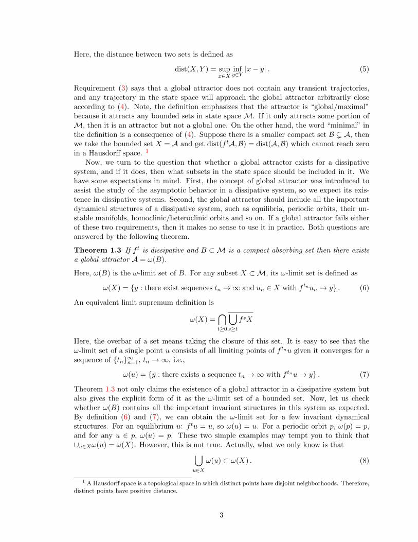
Usually, the left-side set in (8) is much smaller than the right-side set. To illustrate thispoint, Figure 1, taken from [71], depicts a planar system with 3 equilibria {a, b, c}. a and care stable. b has a homoclinic orbit denoted as W u(b) 2 since it is also an unstable manifoldof b. For any u ∈ W u(b), ω(u) = b. However, for the whole orbit ω(W u(b)) = W u(b). Anintuitive explanation goes as follows. For any y ∈W u(b) and a tn > 0, we can find a pointun ahead of y on the homoclinic orbit un ∈ W u(b) such that f tnun = y. The larger tn is,the closer un is to b. It takes an infinitely long time to go backward from y to b. So we findsequences tn →∞ and un ∈W u(b) such that f tnxn → y, and by definition, y ∈ ω(W u(b)).The same argument can be applied to the bounded stable manifold of c in Figure 1(a),ω(W s(c)) = W s(c).

(a) (b)

Figure 1: (a) State space portrait of a 2d system. (b) The corresponding global attractor.

The ω-limit sets of equilibria, periodic orbits, and homoclinic orbits are the objectsthemselves, so they all belong to the global attractor, as we would expect. Meanwhile,concerning the stable and unstable manifolds, we have the following theorem.

Theorem 1.4 The unstable manifolds and bounded stable manifolds of a compact invariantset are contained in the global attractor.

We stress that the global attractor does not contain unbounded stable/unstable manifolds.Unstable manifolds are intrinsically bounded in dissipative systems, so we omit the word“bounded” in front of it in theorem 1.4. The explanation is simple. Let u(t) be a point inthe unstable manifold of an invariant set X, i.e., u(t) ∈W u(X), then u(t) approaches X fort→ −∞ by definition, and u(t) ∈ B when t→∞ because the system is dissipative with Ban absorbing set. Therefore, unstable manifold W u(X) is bounded. However, not all stablemanifolds are bounded. For example, one-dimensional dissipative system u = −λu, λ > 0has a global attractor u = 0, but its stable manifold extends to u→ ±∞. Such a distinctionbetween stable and unstable manifolds in dissipative systems is crucial for us to understandthe finite dimensionality of such systems. In an infinite-dimensional system described by aPDE, an unstable invariant structure usually has only a few unstable modes and the rest,infinite many, are all stable modes. Only a finite subset of these stable modes participatesin the dynamics. As we shall show in this thesis, the rest stable modes are decoupled fromother modes, decay exponentially, and do not belong to the global attractor.

2 The stable and unstable manifolds of a subset X ⊂M are denoted respectively as W s(X) and Wu(X).

4

In the example shown in Figure 1(a), the 3 equilibria {a, b, c}, the stable manifold of c,the homoclinic orbit of b and the heteroclinic orbit from b to a compose the global attractor,which is shown in Figure 1(b).

The global attractor in the Lorenz system We now prove the existence of a globalattractor for the Lorenz system to illustrate the concepts introduced in this section. Theo-rem 1.3 tells us that the key point of showing the existence of a global attractor is to finda compact absorbing set B in the system. For Lorenz system

x = −σx+ σy

y = rx− y − xzz = xy − bz

with σ, r, b > 0, consider

V (x, y, z) = x2 + y2 + (z − r − σ)2 .

Then,

dV

dt= −2σx2 − 2y2 − 2bz2 + 2b(r + σ)z

= −2σx2 − 2y2 − b(z − r − σ)2 − bz2 + b(r + σ)2

≤ −αV + b(r + σ)2

Here α = min(2σ, 2, b). By the Gronwall inequality, we obtain

V ≤ 2b(r + σ)2

α.

Lemma 1.5 (Gronwall’s Inequality) If

du

dt≤ au+ b ,

then

u(t) ≤ (u0 +b

a)eat − b

a.

Therefore, there is an absorbing sphere S with radius (2b/α)1/2(r + σ) in Lorenz system.So a global attractor exists and it is given as ω(S).

1.2.2 The dimension of an attractor

Though the state spaceMmay be infinite-dimensional, after a transient period of evolution,the dynamics is usually determined only by a finite number of degrees of freedom. The globalattractor lives in a finite-dimensional subspace of the state space. Consequently, the studyof the dimension of the global attractor is crucial for us to understand the longtime behaviorof this system. According to ref. [31], the types of dimensions of chaotic attractors can beclassified into three categories. One is fractal dimensions, based purely on the geometry

5

of the attractor such as the box-counting dimension DC and the Hausdorff dimension DH .The second type incorporates the frequency with which a typical trajectory visits variousparts of the attractor, namely the natural measure of the attractor, such as the informationdimension DI , correlation dimension Dµ [46], and so on. The third one, Kaplan-Yorkedimension DKY is defined in terms of the dynamical properties of an attractor rather thanthe geometry or the natural measure. Kaplan and Yorke [38, 51] initially conjecturedthat DKY = DC , but later it was shown that DKY is an upper bound of the informationdimension. Some comparison of these various definitions of dimension can be found inrefs. [31, 46, 49]. In this subsection, we list some representative definitions related to ourresearch.

Box-counting dimension (capacity dimension, Kolmogorov dimension) By usinga minimal set of balls with radius ε to cover the attractor and record the number of ballsN(ε), the box-counting dimension is given by

DC = lim supε→0

logN(ε)

log(1/ε)(9)

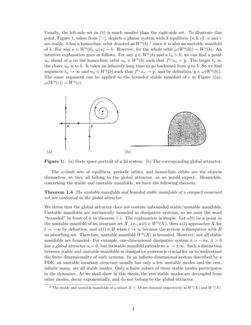
Note, we can also use cubes of side length ε, which does not change the result. Basically,DC tells us how dense the state points are inside the attractor. Trivial cases, like DC = 1for a straight line and DC = 2 for an area, are within our expectation, but for fractalobjects, it usually produces fraction/irrational numbers. For instance, DC = log 3/ log 2 forthe Sierpinski triangle shown in Figure 2.

Figure 2: The iterative process to get the Sierpinski triangle (from ref. [23]).

Hausdorff dimension The box-counting dimension uses balls of the same radius ε tocover the attractor. Here, we try to cover the attractor with nonuniform open balls whoseradius is no larger than ε. First, we define the d-dimensional Hausdorff measure of a set Xin M.

Hd(X) = lim infε→0

{ ∞∑i=0

rdi : ri < ε and X ⊂∞⋃i=0

Bri(ui)

}. (10)

Here, Bri(ui) is a d-dimensional open ball centered at ui with radius ri. The definition isanalogous to the definition of Lebesgue measure. The basic idea is to estimate the volumeof the attractor by the total volume of finer and finer countable d-dimensional coveringballs, where d is a parameter in this measure. If d is larger than the actual dimension of the

6

attractor, then Hd(X) = 0. For example, we need 1/2r circles whose radius is r to cover aunit one-dimensional segment. The total area of these circles goes to zero when r → 0. Onthe other hand, if d is smaller than the actual dimension, then Hd(X)→∞. For instance,we need infinitely long one-dimensional segments to cover a two-dimensional plane. Basedon this observation, the Hausdorff dimension of a compact set X is defined as

DH(X) = inf{d : Hd(X) = 0 with d > 0

}. (11)

In general, the Hausdorff dimension is not easy to get for a dynamical system. But we dohave an upper bound

DH(X) ≤ DC(X) . (12)

This relation is easy to understand. In defining Hausdorff dimension we have more choicesof the covering balls than that in box-counting dimension. Also, (10) is taking an infimumof all choices while DC takes the supremum. For a rigorous proof of (12), see ref. [71].

Information dimension The fractal dimension does not count the frequency with whicheach small region is visited on the attractor. In order to incorporate such information, thenumber of covering balls N(ε) is replaced by the entropy function −∑N(ε) Pi logPi, wherePi is the probability contained in cube ci, namely the natural measure µ(ci) of the attractor.The information dimension is then given as [31]

DI = limε→0

−N(ε)∑i=1

Pi logPi

log(1/ε). (13)

The information dimension is no larger than the box-counting dimension, and DI = DC

when the natural measure is constant across the attractor.

Kaplan-Yorke dimension (Lyapunov dimension) Kaplan and Yorke first proposedthe idea of defining the dimension of a chaotic attractor by the Lyapunov exponents 3 inref. [51], and later they elaborated their proposal it in ref. [38]. Here I sketch their basicidea [73].

Let λ1 ≥ · · · ≥ λn are the Lyapunov spectrum of an n-dimensional chaotic system(λ1 > 0). We try to determine how many cubes needed to cover the neighborhood of atemplate point u(0) as the system evolves. Suppose the neighborhood is an n-dimensionalparallelogram with initially each edge oriented in the covariant direction at u(0), and thenumber of ε-cubes needed to cover this parallelogram is N(ε); then after an infinitesimaltime δt, the neighborhood moves to u(δt) and the parallelogram gets stretched/contractedin each covariant direction. Choose some j + 1 such that λj+1 < 0, we use a smaller cubewith length eλj+1δtε to cover the new neighborhood, then

N(eλj+1δtε) =

(j∏i=1

e(λi−λj+1)δt

)N(ε) (14)

Let’s explain the coefficient above. The ith direction with i < j + 1 has been stretched bya factor eλiδt, and the new cube length is eλj+1δtε, so it needs e(λi−λj+1)δt times more cubes

3Actually, they used the magnitudes of multipliers or the ‘Lyapunov numbers’, defined as the exponentialsof the Lyapunov exponents.

7

along this direction. Also, since choose λj+1 < 0, then for the ith direction with i > j+1, theoriginal number of cubes along this direction is enough to cover it, which means the aboveformula is actually over-counting in this direction. The exponential law N(ε) ∝ ε−d from(9) is valid when ε is small enough. Then (14) reduces to (eλj+1δtε)−d =

∏ji=1 e

(λi−λj+1)δtε−d

and thus

d(j) = j −∑j

i=1 λiλj+1

. (15)

Just as stated above, formula (15) is an upper bound of the dimension. We need to findthe smallest d(j) under condition λj+1 < 0.

d(j + 1)− d(j) = 1−∑j+1

i=1 λiλj+2

+

∑ji=1 λiλj+1

=(λj+2 − λj+1)(λ1 + · · ·+ λj+1)

λj+2λj+1

Let λ1 + · · ·+ λk ≥ 0 and λ1 + · · ·+ λk+1 < 0, then dk+1 > dk and dk < dk−1. Therefore

DKY = k +

∑ki=1 λi|λk+1|

(16)

with k the largest number making λ1 + · · ·+ λk non-negative.

Summary The definitions of dimension introduced in this section provide valuable in-formation about the size of the global attractor. However, except for the Kaplan-Yorkedimension, all the other definitions try to cover the global attractor with cubes statically.The information about the topological structure of a global attractor has not been used. Onthe other hand, strange attractors are almost always fractal, and thus the dimension is anirrational number. With this number, we still do not know how many degrees of freedom areneeded to effectively describe the dynamics of a dissipative PDE in an infinite-dimensionalspace. In the next section, we introduce the concept of the inertial manifold that containsthe global attractor and determines the dynamics by a finite number of degrees of freedom.

1.2.3 Inertial manifold

For dissipative chaotic systems, asymptotic orbits are contained in a lower-dimensionalsubspace of the state space M. Thus the effective dynamics can be described by a finitenumber of degrees of freedom. A global attractor usually has fractal dimension, which makeit hard to analyze, so we need to construct a ‘tight’ smooth manifold that encloses it, andwhose dimension gives the effective degrees of freedom of this system. This is called theinertial manifold [34, 70, 71, 81].

Here we use the concept of “slaving” in order to understand how the transition frominfinite-dimensional space to finite-dimensional subspace happens. Let u(t) be a dynamicalsystem in an infinite-dimensional state space M governed by

du

dt+Au+ F (u) = 0 . (17)

We split the “velocity” field into a linear part and a nonlinear part. Linear operator A isusually a negative Laplace operator or a higher-order spatial derivative. If the nonlinear

8

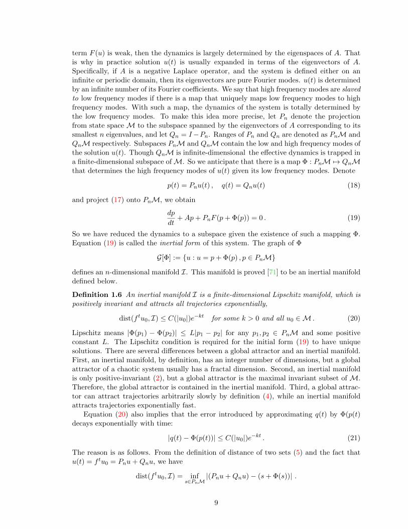
term F (u) is weak, then the dynamics is largely determined by the eigenspaces of A. Thatis why in practice solution u(t) is usually expanded in terms of the eigenvectors of A.Specifically, if A is a negative Laplace operator, and the system is defined either on aninfinite or periodic domain, then its eigenvectors are pure Fourier modes. u(t) is determinedby an infinite number of its Fourier coefficients. We say that high frequency modes are slavedto low frequency modes if there is a map that uniquely maps low frequency modes to highfrequency modes. With such a map, the dynamics of the system is totally determined bythe low frequency modes. To make this idea more precise, let Pn denote the projectionfrom state space M to the subspace spanned by the eigenvectors of A corresponding to itssmallest n eigenvalues, and let Qn = I−Pn. Ranges of Pn and Qn are denoted as PnM andQnM respectively. Subspaces PnM and QnM contain the low and high frequency modes ofthe solution u(t). Though QnM is infinite-dimensional the effective dynamics is trapped ina finite-dimensional subspace ofM. So we anticipate that there is a map Φ : PnM 7→ QnMthat determines the high frequency modes of u(t) given its low frequency modes. Denote

p(t) = Pnu(t) , q(t) = Qnu(t) (18)

and project (17) onto PnM, we obtain

dp

dt+Ap+ PnF (p+ Φ(p)) = 0 . (19)

So we have reduced the dynamics to a subspace given the existence of such a mapping Φ.Equation (19) is called the inertial form of this system. The graph of Φ

G[Φ] := {u : u = p+ Φ(p) , p ∈ PnM}

defines an n-dimensional manifold I. This manifold is proved [71] to be an inertial manifolddefined below.

Definition 1.6 An inertial manifold I is a finite-dimensional Lipschitz manifold, which ispositively invariant and attracts all trajectories exponentially,

dist(f tu0, I) ≤ C(|u0|)e−kt for some k > 0 and all u0 ∈M . (20)

Lipschitz means |Φ(p1) − Φ(p2)| ≤ L|p1 − p2| for any p1, p2 ∈ PnM and some positiveconstant L. The Lipschitz condition is required for the initial form (19) to have uniquesolutions. There are several differences between a global attractor and an inertial manifold.First, an inertial manifold, by definition, has an integer number of dimensions, but a globalattractor of a chaotic system usually has a fractal dimension. Second, an inertial manifoldis only positive-invariant (2), but a global attractor is the maximal invariant subset of M.Therefore, the global attractor is contained in the inertial manifold. Third, a global attrac-tor can attract trajectories arbitrarily slowly by definition (4), while an inertial manifoldattracts trajectories exponentially fast.

Equation (20) also implies that the error introduced by approximating q(t) by Φ(p(t)decays exponentially with time:

|q(t)− Φ(p(t))| ≤ C(|u0|)e−kt . (21)

The reason is as follows. From the definition of distance of two sets (5) and the fact thatu(t) = f tu0 = Pnu+Qnu, we have

dist(f tu0, I) = infs∈PnM

|(Pnu+Qnu)− (s+ Φ(s))| .

9

Since projection Pn and Qn are orthogonal to each other, the above infimum is reachedwhen s = Pnu. Thus we have we

dist(f tu0, I) = |Qnu− Φ(Pnu))| = |q(t)− Φ(p(t))| .

The equivalence between (20) and (21) confirms that the idea of mode slaving works in adissipative system given the existence of an inertial manifold. For any point in the statespace, we can find an approximate state on the inertial manifold. These two states share thesame low frequency modes and only differ in their high frequency modes. High frequencymodes are slaved to low frequency modes, and their difference decays exponentially. Soafter a short transient period, all orbits are effectively captured by the inertial manifold.

An inertial manifold exists in systems which possess the strong squeezing property [71].A system says to have the strong squeezing property if for any two solutions u(t) = p(t)+q(t)and u(t) = p(t) + q(t), the following two properties hold. (i) the cone invariance property :if

|q(0)− q(0)| ≤ |p(0)− p(0)| (22)

then|q(t)− q(t)| ≤ |p(t)− p(t)| (23)

for all t ≤ 0, and (ii) the decay property : if

|q(t)− q(t)| ≥ |p(t)− p(t)| (24)

then|q(t)− q(t)| ≤ |q(0)− q(0)|e−kt (25)

for some k > 0. The first property says that initially if two states satisfy the Lipschitzcondition with Lipschitz constant 1, then such a Lipschitz condition holds at any latertime. The second property accounts for the exponential attraction (20) of the inertialmanifold. In practice, it is hard to verify the strong squeezing property directly. Here weprovide an intuitive argument to show that a large gap in the eigenspectrum of operatorA in (17) leads to the strong squeezing property. Let A have eigenvalues λ1 ≤ λ2 ≤ · · · .Inertial form (19) describes the dynamics of the n low frequency modes which correspondto eigenvalues λ1, · · · , λn. The minimal growth rate in subspace PnM is −λn. While, therest high frequency modes should have approximately the largest growing rate −λn+1. If−λn+1 is far smaller than −λn, then we anticipate that |p(t)− p(t)| should grow faster than|q(t)− q(t)|, so (23) holds. Also, if −λn+1 < 0, then (25) should hold too. Note that we havenot taken into consideration the coupling between low and high frequency modes by thenonlinear term F (u) in (17). Therefore, to ensure strong squeezing property, the thresholdof gap λn+1−λn should depend on F (u). Such a spectral gap condition is precisely describedin the following theorem.

Theorem 1.7 If F (u) is Lipschitz

|F (u)− F (v)| ≤ C1|u− v|, u, v ∈M

and eigenvalues of A in (17) satisfies

λn+1 − λn > 4C1 (26)

for some integer n, then the strong squeezing property holds, with k in (25) satisfying k ≥λn + 2C1.

10

See [71] for the proof of this theorem.The existence of an inertial manifold has been proved for many chaotic or turbulent

systems such as Kuramoto-Sivashinsky equation, complex Ginzburg-Landau equation andthe two-dimensional Navier-Stokes equations [81]. Also, numerical methods such as Euler-Galerkin [36] and nonlinear Galerkin method [61] have been proposed to approximate in-ertial manifolds. Approximating mapping Φ : PnM 7→ QnM requires choosing an appro-priate n first. If n is smaller than the dimension of the inertial manifold, then Φ fails todescribe the inertial manifold. However, if n is far larger than the dimension of the inertialmanifold, then simulations on such approximations to the inertial manifold are not numer-ically efficient. At present, one uses empirical or some test number to truncate the originalsystem. For example, in [36], 3 modes are used to represent the inertial manifold of theone-dimensional Kuramoto-Sivashinsky equation, but this truncated model is not sufficientto preserve the bifurcation diagram. At the same time, mathematical upper bounds for thedimension are not always tight. Therefore, little is known about the exact dimension ofinertial manifolds in dissipative chaotic systems.

1.3 Covariant vectors

The recent progress in numerical methods to calculate covariant vectors [42, 54] has mo-tivated us to explore an inertial manifold by covariant vectors locally through a statisticalstudy of the tangency among covariant vectors [90] and difference vector projection [89].The number of the covariant vectors needed for locally spanning the inertial manifold isregarded as the dimension of an inertial manifold. The key observation in this study is thattangent space can be decomposed into an entangled “physical” subspace and its comple-ment, a contracting disentangled subspace. The latter plays no role in the longtime behavioron the inertial manifold.

In this section, we will introduce covariant vectors (often called “covariant Lyapunovvectors” in the literature [41, 42]) associated with periodic orbits and ergodic orbits. Thegeneral setup is that we have an autonomous continuous flow described by

u = v(u) , u(x, t) ∈ Rn . (27)

The corresponding time-forward trajectory starting from u0 is u(t) = f t(u0). In the linearapproximation, the equation that governs the deformation of an infinitesimal neighborhoodof u(t) (dynamics in tangent space) is

d

dtδu = Aδu , A =

∂v

∂u. (28)

Matrix A is called the stability matrix of the flow. It describes the rates of instantaneousexpansion/contraction and shearing in the tangent space. The Jacobian matrix of the flowtransports linear perturbation along the orbit:

δu(u, t) = J t(u0, 0) δu(u0, 0) (29)

Here we make it explicit that the infinitesimal deformation δu depends on both the orbitand time. The Jacobian matrix is obtained by integrating equation

d

dtJ = AJ , J0 = I . (30)

Jacobian matrix satisfies the semi-group multiplicative property (chain rule) along an orbit,

J t−t0(u(t0), t0) = J t−t1(u(t1), t1)J t1−t0(u(t0), t0) . (31)

11

1.3.1 Floquet vectors

For a point u(t) on a periodic orbit p of period Tp,

Jp = JTp(u, t) (32)

is called the Floquet matrix (monodromy matrix), and its eigenvalues the Floquet multipli-ers Λj . The jth Floquet multiplier is a dimensionless ratio of the final/initial deformationalong the jth eigendirection. It is an intrinsic, local property of a smooth flow, invariantunder all smooth coordinate transformations. The associated Floquet vectors ej(u),

Jp ej = Λjej (33)

define the invariant directions of the tangent space at periodic point u(t) ∈ p. Evolvinga small initial perturbation aligned with an expanding Floquet direction will generate thecorresponding unstable manifold along the periodic orbit. Written in exponential form

Λj = exp(Tpλ(j)p ) = exp(Tpµ

(j) + iθj) ,

where λ(j)p

4 are the Floquet exponents. Floquet multipliers are either real, θj = 0, π, or formcomplex pairs, {Λj ,Λj+1} = {|Λj | exp(iθj), |Λj | exp(−iθj)}, 0 < θj < π. The real parts ofthe Floquet exponents

µ(j) = (ln |Λj |)/Tp (34)

describe the mean contraction or expansion rates per one period of the orbit. Appendix Atalks about the form of the Jacobian matrix of a general linear flow with periodic coefficients.

1.3.2 Covariant vectors

For a periodic orbit, the Jacobian matrix of n periods is the nth power of the Jacobiancorresponding to a single period. However, for an ergodic orbit, there is no such simplerelation. Integrating Jacobian matrix by (30) cannot be avoided for studying asymptoticstability of this orbit. However, similar to Floquet vectors of a periodic orbit, a set ofcovariant vectors exists for an ergodic orbit. Multiplicative ergodic theorem [66, 72] saysthat the forward and backward Oseledets matrices

Ξ±(u) := limt→±∞

[J t(u)>J t(u)]1/2t (35)

both exist for an invertible dynamical system equipped with an invariant measure. Theireigenvalues are eλ

+1 (u) < · · · < eλ

+s (u), and eλ

−1 (u) > · · · > eλ

−s (u) respectively, with λ±i (u) the

Lyapunov exponents (characteristic exponents) and s the total number of distinct exponents(s ≤ n). For an ergodic system, Lyapunov exponents are the same almost everywhere, and

λ+i (u) = −λ−i (u) = λi (36)

The corresponding eigenspaces U±1 (u), · · · , U±s (u) can be used to construct the forward andbackward invariant subspaces:

V +i (u) = U+

1 (u)⊕ · · · ⊕ U+i (u)

V −i (u) = U−i (u)⊕ · · · ⊕ U−s (u) .

4Here, subscript p emphasizes that it is associated with a periodic orbit so as to distinguish it with theLyapunov exponents defined in the next section.

12

u(t0)

u(t1)

u(t2)

u(t3)

stage 1: JiQi = Q

i+1Ri

forward transient

stage 2: JiQi = Qi+1Ri

forward, record

Qi

stage 3: Ci = R−1i Ci+1

backward transientsta

ge 4: Ci

= R−1

iCi+

1

backwa

rd,rec

ordCi

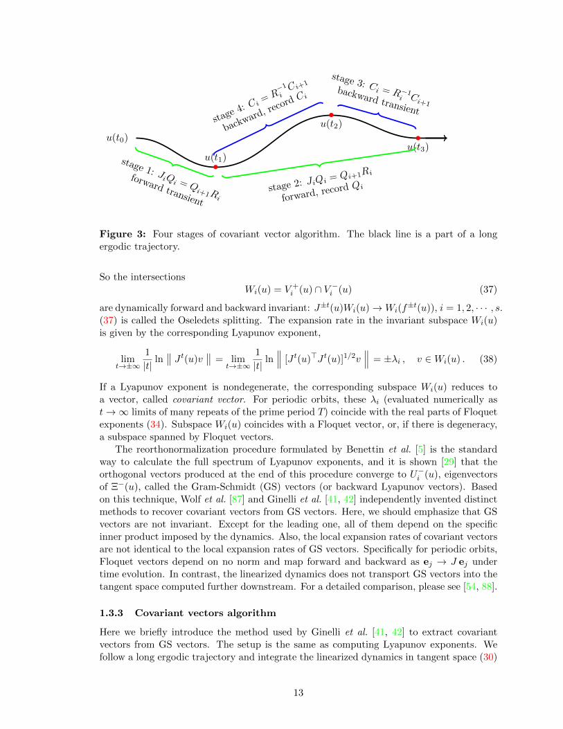
Figure 3: Four stages of covariant vector algorithm. The black line is a part of a longergodic trajectory.

So the intersectionsWi(u) = V +

i (u) ∩ V −i (u) (37)

are dynamically forward and backward invariant: J±t(u)Wi(u)→Wi(f±t(u)), i = 1, 2, · · · , s.

(37) is called the Oseledets splitting. The expansion rate in the invariant subspace Wi(u)is given by the corresponding Lyapunov exponent,

limt→±∞

1

|t| lnww J t(u)v

ww = limt→±∞

1

|t| lnwww [J t(u)>J t(u)]1/2v

www = ±λi , v ∈Wi(u) . (38)

If a Lyapunov exponent is nondegenerate, the corresponding subspace Wi(u) reduces toa vector, called covariant vector. For periodic orbits, these λi (evaluated numerically ast→∞ limits of many repeats of the prime period T) coincide with the real parts of Floquetexponents (34). Subspace Wi(u) coincides with a Floquet vector, or, if there is degeneracy,a subspace spanned by Floquet vectors.

The reorthonormalization procedure formulated by Benettin et al. [5] is the standardway to calculate the full spectrum of Lyapunov exponents, and it is shown [29] that theorthogonal vectors produced at the end of this procedure converge to U−i (u), eigenvectorsof Ξ−(u), called the Gram-Schmidt (GS) vectors (or backward Lyapunov vectors). Basedon this technique, Wolf et al. [87] and Ginelli et al. [41, 42] independently invented distinctmethods to recover covariant vectors from GS vectors. Here, we should emphasize that GSvectors are not invariant. Except for the leading one, all of them depend on the specificinner product imposed by the dynamics. Also, the local expansion rates of covariant vectorsare not identical to the local expansion rates of GS vectors. Specifically for periodic orbits,Floquet vectors depend on no norm and map forward and backward as ej → J ej undertime evolution. In contrast, the linearized dynamics does not transport GS vectors into thetangent space computed further downstream. For a detailed comparison, please see [54, 88].

1.3.3 Covariant vectors algorithm

Here we briefly introduce the method used by Ginelli et al. [41, 42] to extract covariantvectors from GS vectors. The setup is the same as computing Lyapunov exponents. Wefollow a long ergodic trajectory and integrate the linearized dynamics in tangent space (30)

13

with orthonormalization regularly, shown as the first two stages in Figure 3. Here, Ji isthe short-time Jacobian matrix, and Qi+1Ri is the QR decomposition of JiQi. We use thenew generated orthonormal matrix Qi+1 as the initial condition for the next short-timeintegration of (30). Therefore, if we choose an appropriate time length of each integrationsegment, we can effectively avoid numerical instability by repeated QR decomposition. Setthe initial deformation matrix Q0 = I, then after n steps in stage 1, we obtain

Jn−1 · · · J0 = QnRn · · ·R0 .

The diagonal elements of upper-triangular matrices Ri store local Lyapunov exponents,longtime average of which gives the Lyapunov exponents of this system. In stage 1, wediscard all these upper-triangular matrices Ri. We assume that Qi converges to the GSvectors after stage 1, and start to record Ri in stage 2. Since the first m GS vectors spanthe same subspace as the first m covariant vectors, which means

Ti = QiCi . (39)

Here Ti = [W1,W2, · · · ,Wn] refers to the matrix whose columns are covariant vectors atstep i of this algorithm. Ci is an upper-triangular matrix, giving the expansion coefficientsof covariant vectors in the GS basis. Since Ji−1Qi−1 = QiRi, we have Ti = Ji−1Qi−1R

−1i Ci.

Also since Ti−1 = Qi−1Ci−1, we get

Ti = Ji−1Ti−1C−1i−1R

−1i Ci (40)

Since Ti is invariant in the tangent space, namely, Ji−1Ti−1 = TiDi with Di a diagonalmatrix concerning the stretching and contraction of covariant vectors. Substitute it into(40), we get I = DiC

−1i−1R

−1i Ci. Therefore, we obtain the backward dynamics of matrix Ci

:Ci−1 = R−1

i CiDi (41)

Numerically, Di is not formed explicitly since it is only a normalization factor. Ginelliet al. [41, 42] cleverly uncover this backward dynamics and show that Ci converges aftera sufficient number of iterations (stage 3 in Figure 3). We choose an arbitrary upper-triangular matrix as the initial input for the backward iteration (41), Ri are those upper-triangular matrices recorded during stage 2, and R−1

i are also upper-triangular. The productof two upper-triangular matrices is still upper-triangular. Thus, backward iteration (41)guarantees that Ci are all upper-triangular. This process is continued in stage 4 in Figure 3,and Ci are recorded at this stage. For trajectory segment u(t1) to u(t2) in Figure 3, wehave the converged GS basis Qi and the converged Ci, then by (39), we obtain the covariantvectors corresponding to this segment.

Covariant vector algorithm is invented to stratify the tangent spaces along an ergodictrajectory, so it is hard to observe degeneracy numerically. However, for periodic orbits, itis possible that some Floquet vectors form conjugate complex pairs. When this algorithmis applied to periodic orbits, it is reduced to a combination of simultaneous iteration andinverse power iteration; consequently, complex conjugate pairs cannot be told apart. Thismeans that we need to pay attention to the two-dimensional rotation when checking theconvergence of each stage in Figure 3. As is shown in Chapter 5, a complex conjugate pairof Floquet vectors can be extracted from a converged two-dimensional subspace.

14

x x x x x xx x x x x xx x x x x xx x x x x xx x x x x xx x x x x x

x x x x x xx x x x x xx x x x x xx x x x x xx x x x x xx x x x x x

x x x x x xx x x x x xx x x x x xx x x x x xx x x x x xx x x x x x

stage 1−−−−→

x x x x x xx x x x x xx x x x xx x x xx x xx x

x x x x x xx x x x xx x x xx x xx xx

x x x x x xx x x x xx x x xx x xx xx

stage 2−−−−→

x x x x x xx x x x xx x x x x

x x xx xx

x x x x x xx x x x xx x x xx x xx xx

x x x x x xx x x x xx x x xx x xx xx

Figure 4: Two stages of periodic Schur decomposition algorithm illustrated by three [6×6]matrices. Empty locations are zeros.

1.3.4 Periodic Schur decomposition algorithm

Here, we review another algorithm related to our work. The double-implicit-shift QR algo-rithm [84, 85] is the standard way of solving the eigen-problem of a single matrix in manynumerical packages, such as the eig() function in Matlab. Bojanczyk et al. [8] extend thisidea to obtain periodic Schur decomposition of the product of a sequence of matrices. Lateron, Kurt Lust [60] describes the implementation details and provides the correspondingFortran code. On the other hand, by use of the chain rule (31), the Jacobian matrix can bedecomposed into a product of short-time Jacobians with the same dimension. Therefore,periodic Schur decomposition is well suited for computing Floquet exponents.

As illustrated in Figure 4, periodic Schur decomposition proceeds in two stages. First,the sequence of matrices is transformed to the Hessenberg-Triangular form, one of whichhas upper-Hessenberg form while the others are upper-triangular, by a series of Householdertransformations [84]. The second stage tries to diminish the sub-diagonal components ofthe Hessenberg matrix until it becomes quasi-upper-triangular, that is, there are some [2×2]blocks on the diagonal corresponding to complex eigenvalues. The eigenvalues of the matrixproduct are given by the products of all individual matrices’ diagonal elements. However,periodic Schur decomposition is not sufficient for extracting eigenvectors, except the leadingone. Kurt Lust [60] claims to formulate the corresponding Floquet vector algorithm, but tothe best of our knowledge, such an algorithm is not present in the literature. Fortunately,Granat et al. [44] have proposed a method to reorder diagonal elements after periodic Schurdecomposition. This provides an elegant way to compute Floquet vectors as we will see inChapter 5.

1.4 Dynamics averaged over periodic orbits

Statistical properties and the geometrical structure of the global attractor are among themajor questions in the study of chaotic nonlinear dissipative systems. Generally, such asystem will get trapped to the global attractor after a transient period, and we are onlyinterested in the dynamics on the attractor. The intrinsic instability of orbits on the attrac-tor make the longtime simulation unreliable, which is also time-consuming. Fortunately,ergodic theorem [78] indicates that longtime average converges to the same answer as a

15

spatial average over the attractor, provided that a natural measure exists on the attractor.

〈a〉 = limt→∞

1

|M|

∫Mdu0

1

t

∫ t

0dτ a(u(τ)) (42)

=1

|Mρ|

∫Mdu ρ(u) a(u) . (43)

Here, a(u(t)) is an observation, namely, a temporal physical quantity such as average dif-fusion rate, energy dissipation rate, Lyapunov exponents and so on. 〈a〉 refers to its spa-tiotemporal average on the attractor. u(t) defines a dynamical system described by (27).M is the state space of this system. ρ(u) is the natural measure. Normalization quantitiesare

|M| =∫Mdu , |Mρ| =

∫Mdu ρ(u) (44)

We make a distinction between the notation for spatiotemporal average 〈a〉 and that forspatial average

〈a〉 =1

|M|

∫Mdu a(u) .

So if we define the integrated observable

At(u0) =

∫ t

0dτ a(u(τ)) , (45)

then

〈a〉 = limt→∞

1

t〈At〉 = lim

t→∞

1

t

1

|M|

∫Mdu0 A

t(u0) . (46)

Formula (43) provides a nice way to calculate spatiotemporal average while avoiding long-time integration. However, as a strange attractor usually has a fractal structure and thenatural measure ρ(u) could be arbitrarily complicated and non-smooth, computation by(43) is not numerically feasible. This is where the cycle averaging theory [22] enters. Inthis section, we illustrate the process of obtaining the spatiotemporal average (42) by theweighted contributions from a set of periodic orbits.

1.4.1 The evolution operator

Towards the goal of calculating spatiotemporal averages, it does not suffice to follow a singleorbit. Instead, we study a swarm of orbits and see how they evolve as a whole. Equation(46) deploys this idea exactly. We take all points in the state space and evolve them fora certain time, after which we study their overall asymptotic behavior. By formula (46),the spatiotemporal average of observable a(u(t)) is given by the asymptotic behavior of thecorresponding integrated observable At(u). However, instead of calculating 〈At〉, we turnto

〈eβAt〉 =1

|M|

∫Mdus e

βAt(us) . (47)

Here we use us instead of u0 as in (46) to denote the starting point of the trajectory. βis an auxiliary variable. The motivation of studying eβA

tinstead of At will be manifest

later. Actually, this form resembles the partition function in statistical mechanics where

16

β = −1/kT . And we will find several analogous formulas in this section with those in thecanonical ensemble. Equation (47) can be transformed as follows.

〈eβAt〉 =1

|M|

∫Mdus

(∫Mdue δ

(ue − f t(us)

))eβA

t(us) (48)

=1

|M|

∫Mdue

∫Mdus δ

(ue − f t(us)

)eβA

t(us) (49)

=1

|M|∑

all trajectoriesof length t

eβAt(us) . (50)

From (47) to (48), we insert an identity in the integral, and from (48) to (49), we changethe integral order. Here, us and ue denote respectively the starting state and end state ofa trajectory. Basically, (50) says that whenever there is a path from us to ue, we shouldcount its contribution to the spatiotemporal average. This idea is inspired by the pathintegral in quantum mechanics. Feynman interprets the propagator (transition probability)〈ψ(x′, t′)|ψ(x, t)〉 as a summation over all possible paths connecting the starting and endstates, where the classical path is picked out when i/~ → ∞. Here, in (49) we are on abetter standing because the Dirac delta function picks out paths that obey the flow equationexactly. Actually, the transition from a procedural law (42) to a high-level principle (50) isa tendency in physics, similar to the transition from Lagrangian mechanics to the principleof least action, or the transition from Schrodinger equation to the path integral.

The kernel of the integral in (49) is called the evolution operator

Lt(ue, us) = δ(ue − f t(us)

)eβA

t(us) . (51)

The evolution operator shares a lot of similarities with the propagator in quantum mechan-ics. For example, the evolution operator also forms a semigroup:

Lt1+t2(ue, us) =

∫Mdu′ Lt2(ue, u

′)Lt1(u′, us) (52)

We define the action of the evolution operator on a function as

Lt ◦ φ =

∫Mdus Lt(ue, us)φ(us) (53)

which is a function of the end state ue. A function φ(u) is said to be the eigenfunction of Ltif Lt ◦ φ = λ(t)φ. Here λ(t) is the eigenvalue. We make it explicit that it depends on time.Note, Lt acts on a function space, so in principle, Lt is an infinite-dimensional operator.However, in some cases such as piece-wise maps, if the observable is defined uniformly ineach piece of the domain, then Lt can effectively be expressed as a finite-dimensional matrix.Here we give two examples of the eigenfunctions of Lt.

Example 1.1 The invariant measure of an equilibrium is an eigenfunction of Lt The invariantmeasure of an equilibrium uq is given by

φ(u) = δ(u− uq) .

17

Then

Lt ◦ φ =

∫Mdus Lt(ue, us)δ(us − uq)

=

∫Mdus δ

(ue − f t(us)

)eβA

t(us)δ(us − uq)

= δ(ue − f t(uq)

)eβA

t(uq)

= δ(ue − uq) etβa(uq)

= etβa(uq)φ(ue) .

Therefore, the invariant measure of an equilibrium is an eigenfunction of the evolution operator witheigenvalue etβa(uq).

Example 1.2 The invariant measure of a periodic orbit is an eigenfunction of LnT The invariantmeasure of a periodic orbit is given by

φ(u) =1

T

∫ T

0

δ(u− f t(u0)dt . (54)

Here, T is the period of this orbit. u0 is an arbitrarily chosen point on this orbit. Then

LnT ◦ φ =1

T

∫ T

0

∫Mdus δ

(ue − fnT (us)

)eβA

nT (us)δ(us − fnT (u0)dt

=1

T

∫ T

0

∫Mdus δ

(ue − fnT+t(us)

)eβA

nT (ft(u0)δ(us − f t(u0)dt

=1

T

∫ T

0

δ(ue − f t(u0)

)enβA

T (u0)dt

∫Mdus δ(us − f t(u0)

=1

T

∫ T

0

δ(ue − f t(u0)

)enβA

T (u0)dt

= enβAT (u0)φ(ue) .

In the above derivation, we have used the identity AnT (f t(u0) = nAT (u0) which is manifest becauseu0 is a periodic point. In general, (54) is not an eigenfunction of Lt, but it is for t = nT . In the aboveformula, AT (u0) actually does not depend on the choice of the starting point u0 as long as it is onepoint on the periodic orbit.

Let us now turn to the original problem of how to calculate (46) and why we choose theexponential form in (47). Combine (46), (47) and (49), we have

〈a〉 = limt→∞

1

t

∂

∂β〈eβAt〉

∣∣∣∣β=0

(55)

=∂

∂βlimt→∞

1

t

1

|M|

∫Mdue

∫Mdus Lt(ue, us)

∣∣∣∣β=0

. (56)

Here, we have used a trick to obtain the spatial average by using an auxiliary variable β,which is similar to what we do in the canonical ensemble. 〈a〉 is given by the longtimeaverage of the evolution operator. From example 1.1 and 1.2, we see that the eigenvaluesof Lt go to ∞ when t → ∞. Therefore, asymptotically, the leading eigenvalue of Lt willdominate the spatiotemporal average in (56). By the semi-Lie group property (52), we

18

define Lt = etA with A defined as the generator of the evolution operator. Then (56) issimplified as follows,

〈a〉 = limt→∞

1

|M|

∫Mdue

∫Mdus Lt(ue, us)

∂

∂βA∣∣∣∣β=0

(57)

= limt→∞

1

|M|

∫Mdue

∫Mdus δ

(ue − f t(us)

) ∂

∂βA∣∣∣∣β=0

(58)

= limt→∞〈 ∂∂βA〉∣∣∣∣β=0

. (59)

As we said, the time limit above will converge to the leading eigenvalue of A. By letting

s0(β) := the largest eigenvalue of A when t→∞ , (60)

we ultimately reach the formula for spatiotemporal averages,

〈a〉 =∂s0

∂β

∣∣∣∣β=0

. (61)

Equation (61) connects the spatiotemporal averages with the largest eigenvalue of the gen-erator of the evolution operator. It is one of the most important formulas in the cycleaveraging theory. We need to study Lt for t → ∞ to obtain (60). To make calculationseasier, we turn to the resolvent of Lt, i.e., the Laplace transform of Lt.∫ ∞

0dt e−stLt =

1

s−A , Re s > s0 . (62)

So, the leading eigenvalue of A is the pole of the resolvent of the evolution operator. In thenext subsection, we will obtain the expression for the resolvent of Lt by a set of periodicorbits.

1.4.2 Spectral determinants

The discussion in Sect. 1.4.1 motivates us to calculate the leading eigenvalue of the generatorA. Put it in another way, we need to solve equation

det (s−A) = 0 (63)

whose answer gives the full spectrum of A. We claim that spatiotemporal average can becalculated by periodic orbits in this system. Still, there isn’t any hint how (63) is relatedto periodic orbits. On one hand, we see that periodic orbits are related to the trace of theevolution operator by the definition (51).

trLt =

∫Mdu Lt(u, u) =

∫Mdu δ

(u− f t(u)

)eβA

t(u) . (64)

On the other hand, matrix identity

ln detM = tr lnM (65)

19

relates the determinant of a matrix M on the left-hand side in (65) with its trace on theright-hand side. With these two pieces of information, we can express (63) in terms of trLt.

ln det (s−A) = tr ln(s−A) =

∫tr

1

s−A ds . (66)

Also by the definition of resolvent (62), we have

det (s−A) = exp

(∫ds

∫ ∞0

dt e−sttrLt). (67)

The remaining part of this subsection is devoted to calculating∫∞

0 dt e−sttrLt. For a givenperiodic orbit with period Tp, we decompose the trace (64) in two directions: one is parallelto the velocity field u‖ and the other in the transverse direction u⊥,∫ ∞

0dt e−sttrLt =

∫ ∞0

dt e−st∫Mdu⊥ du‖δ

(u⊥ − f t⊥(u)

)δ(u‖ − f t‖(u)

)eβA

t(u) .

We first calculate the integration in the parallel direction. This is a one-dimensionalspatial integration. Due to the periodicity u‖ = f rT‖ (u) for r = 1, 2, · · · , we split theintegration in this parallel direction into infinitely many periods:∫ ∞

0dt e−st

∮pdu‖δ

(u‖ − f t‖(u)

)=

∫ ∞0

dt e−st∫ Tp

0dτ ||v(τ)|| δ

(u‖(τ)− u‖(τ + t)

)(68)

=

∞∑r=1

e−sTpr∫ Tp

0dτ ||v(τ)||

∫ ε

−εdt e−st δ

(u‖(τ)− u‖(τ + rTp + t)

). (69)

The integrand in (69) is defined in a small time window [−ε, ε]. Within this window u‖(τ)−u‖(τ + rT + t) = u‖(τ)− u‖(τ + t) ' −v(τ)t. So if we take ε→ 0,∫ ε

−εdt e−st δ

(u‖(τ)− u‖(τ + rTp + t)

)=

1

‖ v(τ) ‖ .

Therefore, we obtain the integration in the parallel direction,∫ ∞0

dt e−st∮pdu‖δ

(u‖ − f t‖(u)

)= Tp

∞∑r=1

e−sTpr . (70)

Now we calculate the trace integration in the transverse direction. In this case, we areactually integrating on a Poincare section transverse to this periodic orbit. So f t⊥(u) is theprojected evolution function in this section, which has codimension one with the full statespace. Therefore, ∫

Pdu⊥δ

(u⊥ − f rTp⊥ (u)

)=

1∣∣det(1−M r

p

)∣∣ . (71)

Here Mp is the Floquet matrix projected on the Poincare section of this periodic orbit.Combine (70) and (71) and consider all periodic orbits inside this system, we obtain the

trace formula ∫ ∞0

dt e−sttrLt =∑p

Tp

∞∑r=1

er(βAp−sTp)∣∣det(1−M r

p

)∣∣ . (72)

20

Ap is the integrated observable along the orbit for one period. Note, summation∑

p countsall periodic orbits inside this system. Substitute (72) into (67), we obtain the spectraldeterminant

det (s−A) = exp

(−∑p

∞∑r=1

1

r

er(βAp−sTp)∣∣det(1−M r

p

)∣∣)

(73)

of the flow.

1.4.3 Dynamical zeta functions

In the spectral determinant (73),∣∣det

(1−M r

p

)∣∣ is approximately equal to the product ofall the expanding eigenvalues of Mp. That is,

∣∣det(1−M r

p

)∣∣ ' |Λp|r. Here, Λp =∏e Λp,e

is the product of the expanding eigenvalues of the Floquet matrix Mp. The accuracy of thisapproximation improves as r → ∞. Substitute it into the spectral determinant (73), wehave

exp

(−∑p

∞∑r=1

1

r

er(βAp−sTp)

|Λp|r

)= exp

(∑p

ln

(1− eβAp−sTp

|Λp|

))=∏p

(1− eβAp−sTp

|Λp|

),

where we have used the Taylor expansion ln(1 − x) = −∑∞n=1xn

n . Then we obtain thedynamical zeta function,

1/ζ =∏p

(1− tp) , with tp =eβAp−sTp

|Λp|. (74)

Formulas (61), (73) and (74) are the ultimate goal of the discussion in this section.They tell us that the spatiotemporal average is determined by the leading eigenvalue of thegenerator of the evolution operator A, and the eigenspectrum of A can be obtained by thewhole set of periodic orbits inside this system. Formula (73) precisely describes our per-spective on chaotic deterministic flows. The flow on the global attractor can be visualizedas a walk chaperoned by a hierarchy of unstable invariant solutions (equilibria, periodicorbits) embedded in the attractor. An ergodic trajectory shadows one such invariant so-lution for a while, is expelled along its unstable manifold, settles into the neighborhoodof another invariant solution for a while, and repeats this process forever. Together, theinfinite set of these unstable invariant solutions forms the skeleton of the strange attractor,and in fact, spatiotemporal averages can be accurately calculated as a summation takenover contributions from periodic orbits weighted by their stabilities [16, 22].

In practice, we truncate (73) or (74) according to the topological length of periodicorbits, which is primarily established by symbolic dynamics, or if not available, by thestability of periodic orbits. This technique is called cycle expansion, whose effectiveness hasbeen demonstrated in a few one-dimensional maps [3, 4] and ergodic flows [13, 16, 56]. See[22] for more details.

21

CHAPTER II

SYMMETRIES IN DYNAMICAL SYSTEMS

Symmetries play an important role in physics. In the study of pattern formation [20],patterns with different symmetries form under different boundary conditions or initial con-ditions. By considering symmetries only, quite a few prototype equations such as complexGinzburg-Landau equation [2] are proposed and have abundant applications in many fields.So, in general, symmetries help create a wonderful physical world for us. However, in theanalysis of chaotic systems, symmetries introduce drifts of orbits along the symmetry di-rections and thus make the geometrical structure of the global attractor more complicatedthan it really is. In this case, symmetries should be reduced before we conducting anyanalysis. In this chapter, we review the basic notions of group theory, symmetry reductionmethods, and establish the relation between dynamics in the full state space and that inthe symmetry-reduced state space.

2.1 Group theory and symmetries: a review

In quantum mechanics, whenever a system exhibits some symmetry, the correspondingsymmetry group commutes with the Hamiltonian of this system, namely, [U(g), H] =U(g)H−HU(g) = 0. Here U(g) denotes the operation corresponding to symmetry g whosemeaning will be explained soon. The set of eigenstates with degeneracy `, {φ1, φ2, · · · , φ`},corresponding to the same system energy Hψi = Enψi, is invariant under the symmetrysince U(g)ψi are also eigenvectors for the same energy. This information helps us under-stand the spectrum of a Hamiltonian and the quantum mechanical selection rules. Wenow apply the same idea to the classical evolution operator Lt(ue, us) for a system f t(u)equivariant under a discrete symmetry group G = {e, g2, g3, · · · , g|G|} of order |G|:

f t(Dg)u) = D(g) f t(u) for ∀g ∈ G . (75)

We start with a review of some basic facts of the group representation theory. Some exam-ples of good references on this topic are ref. [47, 82].

Suppose group G acts on a linear space V and function ρ(u) is defined on this spaceu ∈ V . Each element g ∈ G will transform point u to D(g)u. At the same time, ρ(u) istransformed to ρ′(u). The value ρ(u) is unchanged after state point u is transformed toD(g)u, so ρ′(D(g)u) = ρ(u). Denote U(g)ρ(u) = ρ′(u), so we have

U(g)ρ(u) = ρ(D(g)−1u) . (76)

This is how functions are transformed by group operations. Note, D(g) is the representationof G in the form of space transformation matrices. The operator U(g), which acts on thefunction space, is not the same as group operation D(g), so (76) does not mean that ρ(u)is invariant under G. Example 2.1 gives the space transformation matrices of C3.

Example 2.1 A matrix representation of cyclic group C3. A 3-dimensional matrix representationof the 3-element cyclic group C3 = {e, C1/3, C2/3} is given by the three rotations by 2π/3 around the

22

z-axis in a 3-dimensional state space,

D(e) =

11

1

, D(C1/3) =

cos 2π3 − sin 2π

3sin 2π

3 cos 2π3

1

,D(C2/3) =

cos 4π3 − sin 4π

3sin 4π

3 cos 4π3

1

.(continued in Example 2.2)

2.1.1 Regular representation

An operator U(g) which acts on an infinite-dimensional function space is too abstract toanalyze. We would like to represent it in a more familiar way. Suppose there is a functionρ(u) with symmetry G defined in full state spaceM, then full state space can be decomposedas a union of |G| tiles each of which is obtained by transforming the fundamental domain,

M =⋃g∈G

gM , (77)

where M is the chosen fundamental domain. So ρ(u) takes |G| different forms by (76) ineach sub-domain in (77). Now, we obtained a natural choice of a set of bases in this functionspace called the regular bases,

{ρreg1 (u), ρreg2 (u), · · · , ρreg|G| (u)} = {ρ(u), ρ(g2u), · · · , ρ(g|G|u)} . (78)

Here, for notation simplicity we use ρ(giu) to represent ρ(D(giu)) without ambiguity. Thesebases are constructed by applying U(g−1) to ρ(u) for each g ∈ G, with u a point in thefundamental domain. The [|G|×|G|] matrix representation of the action of U(g) in bases(78) is called the (left) regular representation Dreg(g). Relation (76) says that Dreg(g) is apermutation matrix, so each row or column has only one nonzero element.

We have a simple trick to obtain the regular representation quickly. Suppose the elementat the ith row and the jth column of Dreg(g) is 1. It means ρ(giu) = U(g)ρ(gj u), which isgi = g−1gj =⇒ g−1 = gig

−1j . Namely,

Dreg(g)ij = δg−1, gig−1j. (79)

So if we arrange the columns of the multiplication table by the inverse of the group elements,then setting positions with g−1 to 1 defines the regular representation Dreg(g). Note, theabove relation can be further simplified to g = gjg

−1i , but it exchanges the rows and columns

of the multiplication table, so g = gjg−1i should not be used to get Dreg(g). On the other

hand, it is easy to see that the regular representation of group element e is always theidentity matrix.

Example 2.2 The regular representation of cyclic group C3. (continued from Example 2.1) Takean arbitrary function ρ(u) over the state space u ∈ M, and define a fundamental domain M as a 1/3wedge, with axis z as its (symmetry invariant) edge. The state space is tiled with three copies of thewedge,

M = M1 ∪ M2 ∪ M3 = M ∪ C1/3M ∪ C2/3M .

23

Table 1: The multiplication tables of the (a) group C2 and (b) C3.

(a)

C2 e σ−1

e e σσ σ e

(b)

C3 e (C1/3)−1 (C2/3)−1

e e C2/3 C1/3

C1/3 C1/3 e C2/3

C2/3 C2/3 C1/3 e

Function ρ(u) can be written as the 3-dimensional vector of functions over the fundamental domainu ∈ M,

(ρreg1 (u), ρreg2 (u), ρreg3 (u)) = (ρ(u), ρ(C1/3u), ρ(C2/3u)) . (80)

The multiplication table of C3 is given in Table 1. By (79), the regular representation matrices Dreg(g)have ‘1’ at the location of g−1 in the multiplication table, ‘0’ elsewhere. The actions of the operatorU(g) are now represented by permutations matrices (blank entries are zeros):

Dreg(e) =

11

1

, Dreg(C1/3) =

11

1

, Dreg(C2/3) =

11

1

. (81)

Table 2: The multiplication table of D3, the group of symmetries of an equilateral triangle.

D3 e (σ12)−1 (σ23)−1 (σ31)−1 (C1/3)−1 (C2/3)−1

e e σ12 σ23 σ31 C2/3 C1/3

σ12 σ12 e C1/3 C2/3 σ31 σ23

σ23 σ23 C2/3 e C1/3 σ12 σ31

σ31 σ31 C1/3 C2/3 e σ23 σ12

C1/3 C1/3 σ31 σ12 σ23 e C2/3

C2/3 C2/3 σ23 σ31 σ12 C1/3 e

Example 2.3 The regular representation of dihedral group D3. D3 = {e, σ12, σ23, σ31, C1/3, C2/3}represents the symmetries of a triangle with equal sides. C1/3 and C2/3 are rotations by 2π/3 and 4π/3respectively. σ12, σ23 and σ31 are 3 reflections. The regular bases in this case are(

ρ(u), ρ(σ12u), ρ(σ23u), ρ(σ31u), ρ(C1/3u), ρ(C2/3u)).

It helps us obtain the multiplication table quickly by the following relations

σ31 = C1/3σ12 , σ23 = C2/3σ12 , C1/3σ12 = σ12C2/3 , C2/3σ12 = σ12C

1/3 . (82)

The multiplication table of D3 is given in Table 2. By (79), the 6 regular representation matricesDreg(g) have ‘1’ at the location of g−1 in the multiplication table, ‘0’ elsewhere. For example, theregular representation of the action of operators U(σ23) and U(C2/3) are, respectively:

Dreg(σ23) =

0 0 1 0 0 00 0 0 0 0 11 0 0 0 0 00 0 0 0 1 00 0 0 1 0 00 1 0 0 0 0

, Dreg(C1/3) =

0 0 0 0 1 00 0 0 1 0 00 1 0 0 0 00 0 1 0 0 00 0 0 0 0 11 0 0 0 0 0

.

24

2.1.2 Irreducible representations

U(g) is a linear operator under the regular bases. Any linearly independent combination ofthe regular bases can be used as new bases, and then the representation of U(g) changesrespectively. So we ask a question: can we find a new set of bases

ρirri =∑j

Sijρregj (83)

such that the new representation Dirr(g) = SDreg(g)S−1 is block-diagonal for any g ∈ G ?

Dirr(g) =

D(1)(g)

D(2)(g). . .

=

r⊕µ=1

dµD(µ)(g) . (84)

In such a block-diagonal representation, the subspace corresponding to each diagonal blockis invariant under G and the action of U(g) can be analyzed subspace by subspace. It can beeasily checked that for each µ, D(µ)(g) for all g ∈ G form another representation (irreduciblerepresentation, or irrep) of group G. Here, r denotes the total number of irreps of G. Thesame irrep may show up more than once in the decomposition (84), so the coefficient dµdenotes the number of its copies. Moreover, it is proved [47] that dµ is also equal to thedimension of D(µ)(g) in (84). Therefore, we have a relation

r∑µ=1

d2µ = |G| .

Example 2.4 Irreps of cyclic group C3. (continued from Example 2.2) For C2 whose multiplicationtable is in Table 1, we can form the symmetric base ρ(u)+ρ(σu) and the antisymmetric base ρ(u)−ρ(σu).You can verify that under these new bases, C2 is block-diagonalized. We would like to generalize thissymmetric-antisymmetric decomposition to the order 3 group C3. Symmetrization can be carried out onany number of functions, but there is no obvious anti-symmetrization. We draw instead inspiration fromthe Fourier transformation for a finite periodic lattice, and construct from the regular bases (80) a newset of bases

ρirr0 (u) =1

3

[ρ(u) + ρ(C1/3u) + ρ(C2/3u)

](85)

ρirr1 (u) =1

3

[ρ(u) + ω ρ(C1/3u) + ω2ρ(C2/3u)

](86)

ρirr2 (u) =1

3

[ρ(u) + ω2ρ(C1/3u) + ω ρ(C2/3u)

]. (87)

Here ω = e2iπ/3. The representation of group C3 in this new bases is block-diagonal by inspection:

Dirr(e) =

11

1

, Dirr(C1/3) =

1 0 00 ω 00 0 ω2

, Dirr(C2/3) =

1 0 00 ω2 00 0 ω

. (88)

So C3 has three 1-dimensional irreps. Generalization to any Cn is immediate: this is just a finite latticeFourier transform.

25

Character tables. Finding a transformation S which simultaneously block-diagonalizesthe regular representation of each group element sounds difficult. However, suppose it canbe achieved and we obtain a set of irreps D(µ)(g), then according to Schur’s lemmas [47],D(µ)(g) must satisfy a set of orthogonality relations:

dµ|G|

∑g

D(µ)il (g)D

(ν)mj(g

−1) = δµνδijδlm . (89)

Denote the trace of irrep D(µ) as χ(µ), which is referred to as the character of D(µ). Prop-erties of irreps can be derived from (89), and we list them as follows:

1. The number of irreps is the same as the number of classes.

2. Dimensions of irreps satisfy∑r

µ=1 d2µ = |G|

3. Orthonormal relation I :∑r

i=1 |Ki|χ(µ)i χ

(ν)∗i = |G|δµν .

Here, the summation goes through all classes of this group, and |Ki| is the number ofelements in class i. This weight comes from the fact that elements in the same classhave the same character. Symbol ∗ means the complex conjugate.

4. Orthonormal relation II :∑r

µ=1 χ(µ)i χ

(µ)∗j = |G|

|Ki|δij .

The characters for all classes and irreps of a finite group are conventionally arranged into acharacter table, a square matrix whose rows represent different classes and columns representdifferent irreps. Rules 1 and 2 help determine the number of irreps and their dimensions.As the matrix representation of class {e} is always the identity matrix, the first row isalways the dimension of the corresponding representation. All entries of the first column arealways 1, because the symmetric irrep is always one-dimensional. To compute the remainingentries, we should use properties 3, 4 and the class multiplication tables. Spectroscopistsconventions use labels A and B for symmetric, respectively antisymmetric nondegenerateirreps, and E, T , G, H for doubly, triply, quadruply, quintuply degenerate irreps.

Table 3: Character tables of C2, C3 and D3. The classes {σ12, σ13, σ14}, {C1/3, C2/3} aredenoted 3σ, 2C, respectively.

C2 A B

e 1 1σ 1 -1

C3 A E

e 1 1 1

C1/3 1 ω ω2

C2/3 1 ω2 ω

D3 A B E

e 1 1 23σ 1 -1 02C 1 1 -1

Example 2.5 Character table of D3. (continued from Example 2.3) Let us construct Table 3.one-dimensional representations are denoted by A and B, depending on whether the basis function issymmetric or antisymmetric with respect to transpositions σij . E denotes the two-dimensional represen-tation. As D3 has 3 classes, the dimension sum rule d21 +d22 +d23 = 6 has only one solution d1 = d2 = 1,d3 = 2. Hence there are two one-dimensional irreps and one two-dimensional irrep. The first row is 1, 1, 2,and the first column is 1, 1, 1 corresponding to the one-dimensional symmetric representation. We taketwo approaches to figure out the remaining 4 entries. First, since B is an antisymmetric one-dimensionalrepresentation, so the characters should be ±1. We anticipate χB(σ) = −1 and can quickly figure outthe remaining 3 positions. Then we check that the obtained table satisfies the orthonormal relations.

26

Second, denote χB(σ) = x and χE(σ) = y, then from the orthonormal relation of the second columnwith the first column and itself, we obtain 1 + x+ 2y = 0 and 1 + x2 + y2 = 6/3. Then we get two setsof solutions, one of which is incompatible with other orthonormal relations, so we are left with x = −1,y = 0. Similarly, we can get the other two characters.

2.1.3 Projection operator

We have listed the properties of irreps and the techniques of constructing a character table,but we still do not know how to construct the similarity transformation S which takes aregular representation into a block-diagonal form. Think of it in another way, each irrep isassociated with an invariant subspace, so by projecting an arbitrary function ρ(u) into itsinvariant subspaces, we find the transformation (83). One of these invariant subspaces is∑

g ρ(gu), which is the basis of the one-dimensional symmetric irrep A. For C3, it is (85).But how to get the others? We resort to the projection operator:

P(µ)i =

dµ|G|

∑g

(D

(µ)ii (g)

)∗U(g) . (90)

It projects an arbitrary function into the ith basis of irrep D(µ) provided the diagonal

elements of this representation D(µ)ii are known. P

(µ)i ρ(u) = ρ

(µ)i . Here, symbol ∗ means the

complex conjugate. For unitary groups(D

(µ)ii (g)

)∗= D

(µ)ii (g−1). Summing i in (90) gives

P (µ) =dµ|G|

∑g

(χ(µ)(g)

)∗U(g) . (91)

This is also a projection operator which projects an arbitrary function onto the sum of thebases of irrep D(µ).

Note, for one-dimensional representations, (91) is equivalent to (90). The projection op-erator is known after we obtain the character table, since the character of an one-dimensionalmatrix is the matrix itself. However, for two-dimensional or higher-dimensional represen-

tations, we need to know the diagonal elements D(µ)ii in order to get the bases of invariant

subspaces. That is to say, (90) should be used instead of (91) in this case. Example 2.6illustrates this point. The two one-dimensional irreps are obtained by (91), but the otherfour two-dimensional irreps are obtained by (90).

Example 2.6 Bases for irreps of D3. (continued from Example 2.3) We use projection operator(91) to obtain the bases of irreps of D3. From Table 3, we have

PAρ(u) =1

6

[ρ(u) + ρ(σ12u) + ρ(σ23u) + ρ(σ31u) + ρ(C1/3u) + ρ(C2/3u)

](92)

PBρ(u) =1

6

[ρ(u)− ρ(σ12u)− ρ(σ23u)− ρ(σ31u) + ρ(C1/3u) + ρ(C2/3u)

]. (93)

For projection into irrep E, we need to figure out the explicit matrix representation first. Obviously, thefollowing 2 by 2 matrices are E irreps.

DE(e) =

[1 00 1

], DE(C1/3) =

[ω 00 ω2

], DE(C2/3) =

[ω2 00 ω

](94)

DE(σ12) =

[0 11 0

], DE(σ23) =

[0 ω2

ω 0

], DE(σ31) =

[0 ωω2 0

]. (95)

27

So apply projection operator (90) on ρ(u) and ρ(σ12u), we get

PE1 ρ(u) =1

6

[ρ(u) + ωρ(C1/3u) + ω2ρ(C2/3u)

](96)

PE2 ρ(u) =1

6

[ρ(u) + ω2ρ(C1/3u) + ωρ(C2/3u)

](97)

PE1 ρ(σ12u) =1

6

[ρ(σ12u) + ωρ(σ31u) + ω2ρ(σ23u)

](98)

PE2 ρ(σ12u) =1

6

[ρ(σ12u) + ω2ρ(σ31u) + ωρ(σ23u) .

](99)

The above derivation has used formulas (82). Under the invariant bases{PAρ(u), PBρ(u), PE1 ρ(u), PE2 ρ(σ12u), PE1 ρ(σ12u), PE2 ρ(u)

},

we have

Dirr(σ23) =

1 0 0 0 0 00 −1 0 0 0 00 0 0 ω2 0 00 0 ω 0 0 00 0 0 0 0 ω2

0 0 0 0 ω 0

Dirr(C1/3) =

1 0 0 0 0 00 1 0 0 0 00 0 ω 0 0 00 0 0 ω2 0 00 0 0 0 ω 00 0 0 0 0 ω2

.The C3 and D3 examples used in this section can be generalized to any Cn and Dn. For

references, Example 2.7, Example 2.8 and Example 2.9 give the character tables of Cn andDn.

Example 2.7 Character table of cyclic group Cn. The symmetry under a discrete rotation by angle2π/n gives birth to a cyclic group Cn = {e, Cn, C2

n, · · · , Cn−1n }. Since Cn is Abelian, each elementforms a separate class, and thus Cn has n one-dimensional irreducible representations. The charactersmultiply as group elements: χα(Cin)χα(Cjn) = χα(Ci+jn ) mod n . Therefore, we get Table 4.

Table 4: Character table of cyclic group Cn. Here k, j = 1, 2, · · · , n− 1.

Cn A Γje 1 1

Ckn 1 exp( i2πkjn )

Example 2.8 Character table of dihedral group Dn = Cnv, n odd. The Dn group

Dn = {e, Cn, C2n, · · · , Cn−1n , σ, Cnσ, · · · ,Cn−1n σ}

has n rotation elements and n reflections. Group elements satisfies Cin · Cjnσ = Cjnσ · Cn−in , so Cin andCn−in form a class. Also, Cn−in ·C2i+j

n σ = Cjnσ ·Cn−in implies that Cjnσ and C2i+jn σ are in the same class.

Therefore, there are only three different types of classes: {e}, {Ckn, Cn−kn } and {σ,Cnσ, · · · ,Cn−1n σ}.The total number of classes is (n+ 3)/2. In this case, there are 2 one-dimensional irreducible representa-tions (symmetric A1 and anti-symmetric A2 ) and (n−1)/2 two-dimensional irreducible representations.In the jth two-dimensional irreducible representation, class {e} has form

(1 00 1

), class {Ckn, Cn−kn } has

form( exp( i2πkjn ) 0

0 exp(− i2πkjn )

), and class {σ,Cnσ, · · · ,Cn−1n σ} has form

(0 11 0

). We get Table 5.

Example 2.9 Character table of dihedral group Dn = Cnv, n even. In this case, there are (n+6)/2 classes: {e}, {C1/2}, {Ck/n, C(n−k)/n}, {σ, σC2/n, · · · , σC(n−2)/n} and {σC1/n, σC3/n, · · · , σC(n−1)/n}.There are four different one-dimensional irreducible representations, whose characters are ±1 under re-flection σ and shift-reflect operation σC1/n. We get Table 6.

28

Table 5: Character table of dihedral group Dn = Cnv, n odd.

Dn (n odd) A1 A2 Eje 1 1 2

Ckn, Cn−kn 1 1 2 cos(2πkj

n )σ, σC1

n, · · · , σCn−1n 1 -1 0

Table 6: Character table of dihedral group Dn = Cnv, n even. Here k, j = 1, 2, · · · , n− 1.

Dn (n even) A1 A2 B1 B2 Eje 1 1 1 1 2

C1/2 1 1 (−1)n/2 (−1)n/2 2(−1)j

Ck/n, C(n−k)/n (k odd) 1 1 -1 -1 2 cos(2πkjn )

Ck/n, C(n−k)/n (k even) 1 1 1 1 2 cos(2πkjn )

σ, σC2/n, · · · , σC(n−2)/n 1 -1 1 -1 0

σC1/n, σC3/n, · · · , σC(n−1)/n 1 -1 -1 1 0

2.2 Symmetry reduction for dynamical systems

In a dynamical system with discrete or continuous symmetries, points in the state spacewhich are related to each other by symmetry operation should be treated as a group.Each member of this group has the same dynamical properties, so we say that they aredynamically equivalent. It is a good practice to choose a single representative in eachgroup and study the dynamics of this representative point instead. This treatment is calledsymmetry reduction. The new state space that this representative point lives in is calledthe (symmetry-)reduced state space After it was invented, symmetry reduction becomesextremely successful for simplifying the analysis of a dynamical system with symmetries. Inthis section, we will discuss symmetry reduction techniques and study the tangent dynamicsin the reduced state space.

2.2.1 Continuous symmetry reduction

We use the same setup as in Sect. 1.3 and copy a few equations here for convenience. Thecontent of this subsection is based on the materials in [22]. Let u = v(u) , u(x, t) ∈ Rndefine a flow. Usually we omit the dependence on coordinates, and write u(t). Denote theevolution semigroup of this flow by u(t) = f t(u0). We say that this flow is equivariant undera continuous symmetry group G if

gv(u) = v(gu) , gf t(u) = f t(gu) for any g ∈ G . (100)

The two equations above are equivalent. In practical applications, G is always a Lie group.Basically, (100) means that if two starting states, which are related to each other by a groupoperation, evolve for the same period of time, then the end states are related by the samegroup operation.

Now we introduce the terminology that will be used in the later discussion. In is often

29

more convenient to write the Lie group G in its exponential form

g(φ) = eφ ·T , φ ·T =

s∑a=1

φaTa , (101)

where Ta, a = 1, 2 · · · , s are the generators of G, and φa are the parameters of this group.Dot product refers to a sum over generators in this section. Generators of a real represen-tation are antisymmetric:

Ta> = −Ta , (102)

where Ta> denotes the transpose of Ta. Let’s work out a simple example. The translation

group {g : g(x0)u(x, t) = u(x + x0, t)} is denoted as g(x0) = exp(x0∂∂x). Here, ∂

∂x is theonly generator and x0 is the parameter. Furthermore, we assume that the generators ofg(φ) commute with each other: TaTb = TbTa.

We define the group orbit of a point u as

Orb(u) = {g u : g ∈ G} . (103)

A group orbit is an s-dimensional manifold, but it is not a real orbit. It is a collection ofall dynamically equivalent points. The group tangent of state u is defined as

ta(u)i = (Ta)ijuj , (104)

which is basically a matrix-vector product. Note, (100) says that the flow equation isequivariant under G, but it does not mean that any orbit in the state space possesses allsymmetries in G. Now we define several important invariant structures.

Equilibrium u(t) = u(0). Namely, v(u) = 0.

Relative equilibrium A state point u(x, t) is a relative equilibrium if

u(t) = g(t c)u(0) = et c·Tu(0) , (105)

where c is a constant. Definition (105) is equivalent to v(u) = c ·t(u). A relative equilibriumis very similar to an equilibrium except for a constant drifting in the group direction.

Periodic orbit u(Tp) = u(0). Tp is the period.

Relative periodic orbit Similar to periodic orbits, if a state returns to its initial stateexcept for a group translation after a center time, then we say that this point is on a relativeperiodic orbit.

up(0) = gpup(Tp) , (106)

where Tp is the period. gp = g(φp) takes the end state to the initial state. We use subscriptp to indicate that the variable belongs to a periodic orbit or relative periodic orbit.

With the above setup, we illustrate how to use slice to reduce continuous symmetries.The idea is similar to a Poincare section. We define a slice that cuts every group orbit onlyonce, so that we can use this intersection point as the representative of the whole grouporbit. The simplest slice is a flat hypersurface that is normal to the group tangent of apre-specified point u′:

〈u− u′|t′a〉 = 〈u|t′a〉 = 0 , t′a = ta(u′) = Ta u

′ , for a = 1, 2, · · · , s . (107)

30

Here, we use a bra-ket notation for the inner product of two real vectors in Rn,

〈u|w〉 = u>w =n∑i=1

uiwi .

A hat on a state indicates that it is a state in the symmetry-reduced state space. Definition(107) has used 〈u′|t′a〉 = 〈u′|Ta u

′〉 = 0 which is the result of the antisymmetry of Ta (102).Now, symmetry reduction turns out to be a process of finding a specific group element g(φ)that transforms each state u into the slice.

u = g−1(φ)u . (108)

u is the state on the slice that represents u and the whole group orbit of u. Note, it usuallyrequires different group parameter φ for different states in (108). Equivalently, we canrecover the state in the full state space by the state in the symmetry-reduced state spaceand the group parameter φ,

u = g(φ) u . (109)

The symmetry reduction process described above is called the post-processing method.That is, we need to know the trajectory beforehand in order to reduce it into the slice.However, many a time, it is more efficient to integrate the system in the slice directly. Thisposts a question of what the dynamics is like in the slice. Let us start from finding thereduced velocity in the slice. Take the time derivative of both sides of (109), v(gu) = v(u) =gu+ gv. Rewrite it with v = g−1v(g u)− g−1g u and the equivariance condition (100) leadsto v = v − g−1g u. Also, by (101) and the definition of the group tangent (104), we get

g−1g u =s∑

a=1

φa(u) Tau =s∑

a=1

φa(u)ta(u) .

So the velocity in the slice is given as

v(u) = v(u) −s∑

a=1

φa(u)ta(u) (110)

The dynamics of φa(u) is governed by the slice. Taking the time derivative of the slicecondition (107) and substituting (110), we get

〈t′a|v(u)〉 = 〈t′a|v(u)〉 −s∑b=1

〈t′a|tb(u)〉 φb = 0 , for a = 1, 2, · · · , s .

This defines s linear equations with total s unknowns. Define the coefficient matrix as Lwhose element is

L(u)ab = 〈t′a|tb(u)〉 , (111)

then we can solve the equation for φa(u). In summary, the dynamics in the slice is governedby

v(u) = v(u) −s∑

a=1

φa(u)ta(u) , u ∈ M (112)

φa(u) =

s∑b=1

(L−1)ab〈t′b|v(u)〉 , a = 1, 2, · · · , s . (113)

31

The above in-slice dynamics fails when L is singular. One obvious cause of failure is asituation where some t′a are parallel. So when choosing the template points for defining theslice, we need to guarantee that t′a, a = 1, 2, · · · , s are not parallel. Under this assumption,a slice fails only when the in-slice state u makes (111) singular. The set of these pointsdefines the border of the slice.

When the group has only one parameter φ, then matrix L is a scalar and the aboveformula can be simplified as

v(u) = v(u) − φ(u)t(u) , u ∈ M (114)

φ(u) = 〈v(u)|t′〉/〈t(u)|t′〉 . (115)

2.2.2 Tangent dynamics in the slice

Equations (112)(113) or (114)(115) describe the dynamics in the slice, by which we canobtain the whole in-slice trajectory given a starting in-slice state. However, sometimes wenot only desire the in-slice orbit but also the tangent dynamics in the slice. More precisely,formulas (28) and (30) describe the tangent dynamics in the full state space. What arethe corresponding formulas in the slice? What is the relation between Jacobian matrix inthe slice and that in the full state space? This subsection is devoted to answering thesequestions. For simplicity, in the following, we assume that the continuous group has onlyone parameter, i.e., s = 1 in (101). Nevertheless, the technique described below can beeasily extended to symmetries with more than one group parameter.

g−1(φ1) g−1(φ2)

δu(t1)

δu(t2)

δu(t1)

δu(t2)

Figure 5: The relation between deformations in the full state space and in the slice. Thepink plane is the slice. The black curve is a trajectory in the state space. The cyan curveis the corresponding trajectory in the slice. Infinitesimal deformation δu(t1) at time t1 istransported to δu(t2) at time t2. δu(t1) and δu(t2) are the in-slice correspondents.

First, we investigate how infinitesimal deformation is transformed into the slice fromthe full state space. We start from the slice condition (107). Infinitesimal deformation δuat u should be confined to the slice too, so we have a constraint

〈δu|t′〉 = 0 . (116)

32

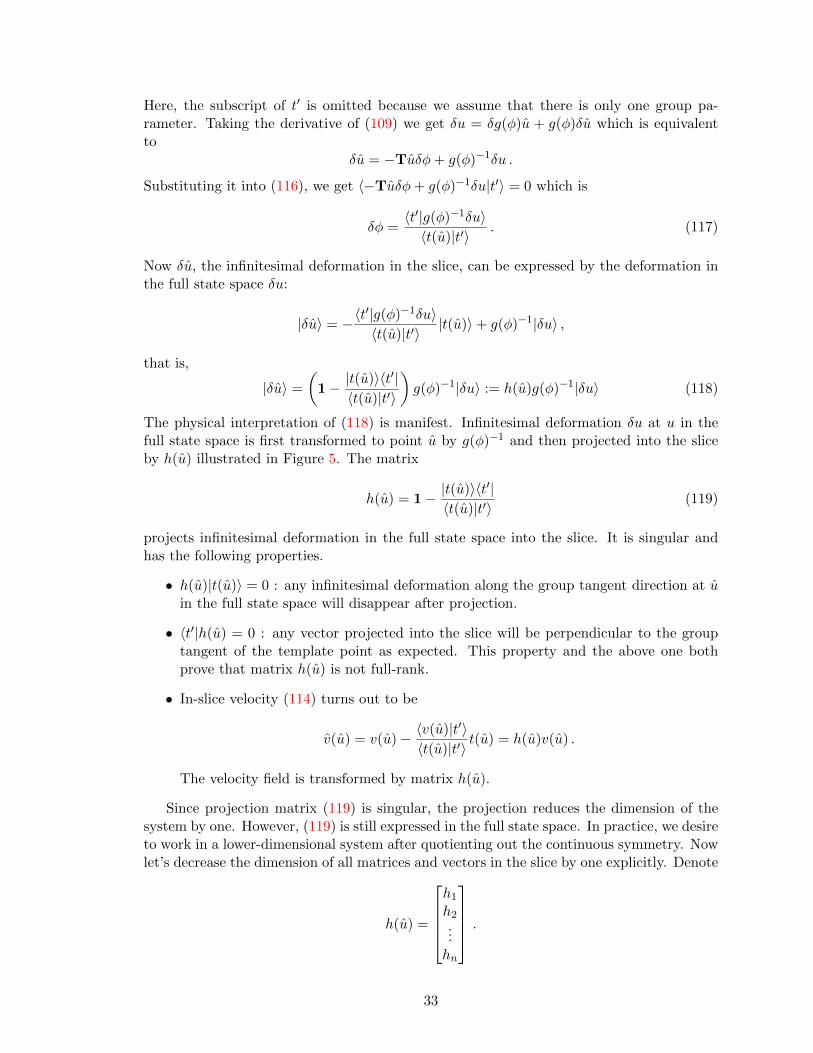
Here, the subscript of t′ is omitted because we assume that there is only one group pa-rameter. Taking the derivative of (109) we get δu = δg(φ)u + g(φ)δu which is equivalentto

δu = −Tuδφ+ g(φ)−1δu .

Substituting it into (116), we get 〈−Tuδφ+ g(φ)−1δu|t′〉 = 0 which is

δφ =〈t′|g(φ)−1δu〉〈t(u)|t′〉 . (117)

Now δu, the infinitesimal deformation in the slice, can be expressed by the deformation inthe full state space δu:

|δu〉 = −〈t′|g(φ)−1δu〉〈t(u)|t′〉 |t(u)〉+ g(φ)−1|δu〉 ,

that is,

|δu〉 =

(1− |t(u)〉〈t′|

〈t(u)|t′〉

)g(φ)−1|δu〉 := h(u)g(φ)−1|δu〉 (118)

The physical interpretation of (118) is manifest. Infinitesimal deformation δu at u in thefull state space is first transformed to point u by g(φ)−1 and then projected into the sliceby h(u) illustrated in Figure 5. The matrix

h(u) = 1− |t(u)〉〈t′|〈t(u)|t′〉 (119)

projects infinitesimal deformation in the full state space into the slice. It is singular andhas the following properties.

• h(u)|t(u)〉 = 0 : any infinitesimal deformation along the group tangent direction at uin the full state space will disappear after projection.

• 〈t′|h(u) = 0 : any vector projected into the slice will be perpendicular to the grouptangent of the template point as expected. This property and the above one bothprove that matrix h(u) is not full-rank.

• In-slice velocity (114) turns out to be

v(u) = v(u)− 〈v(u)|t′〉〈t(u)|t′〉 t(u) = h(u)v(u) .

The velocity field is transformed by matrix h(u).

Since projection matrix (119) is singular, the projection reduces the dimension of thesystem by one. However, (119) is still expressed in the full state space. In practice, we desireto work in a lower-dimensional system after quotienting out the continuous symmetry. Nowlet’s decrease the dimension of all matrices and vectors in the slice by one explicitly. Denote

h(u) =

h1

h2...hn

.

33

Each hi is a row vector and n is the dimension of the full state space. From the secondproperty of h(u) we know that hi are linear dependent: t′1h1 + t′2h2 + · · ·+ t′nhn = 0. Heret′i are components of vector t′. Assume t′ξ 6= 0, then

hξ =

n∑i=1,i6=ξ

− t′i

t′ξhi

so hξ can be eliminated from h(u):

h(u) =

11

. . .

− t′1t′ξ− t′2t′ξ

· · · − t′nt′ξ

. . .

1

︸ ︷︷ ︸

n×(n−1)

h1...

hξ−1

hξ+1...hn

︸ ︷︷ ︸(n−1)×n

:= P ′h(−)(u) .

The above expression is the rank factorization of h(u) with h(−)(u) a full-rank matrix. Thesuperscript of the minus sign indicates that the matrix (vector) is (n − 1)-dimensional.Similarly, from the slice condition 〈t′|u〉 = 0, we can reduce the dimension of a point on theslice by one

u = P ′u(−)

and also reduce the dimension of an infinitesimal deformation by one

δu = P ′δu(−) .

Here, u(−) and δu(−) are both (n− 1)-dimensional vectors.

u(−) = [u1, · · · , uξ−1, uξ+1, · · · , un]> , δu(−) = [δu1, · · · , δuξ−1, δuξ+1, · · · , δun]> .

Now relation (118) can be rewritten as:

|δu(−)〉 = h(−)(u)g(φ)−1|δu〉 (120)

Note that the left side of the above equation is an (n−1)-dimensional vector while the rightside |δu〉 is an n-dimensional vector and the [(n− 1)×n] matrix h(−)(u) is the “projection”operator.

2.2.3 In-slice Jacobian matrix

Now let’s turn to the transformation of the Jacobian matrix. In Figure 5, there is a tra-jectory from u(t1) to u(t2) in the full state space. The corresponding transformed in-slicetrajectory is from u(t1) to u(t2). Infinitesimal deformations in the full state space and inthe slice will be evolved by the Jacobian matrix in the full state space and in the slicerespectively.

Jδu(t1) = δu(t2) (121)

Jδu(−)(t1) = δu(−)(t2) . (122)

34

Here, J = J t2−t1(u(t1), t1) and J = J t2−t1(u(−)(t1), t1). For notation simplicity, we omit allparameters of Jacobian matrix if no confusion occurs. Substituting (120) into (122), we get

Jh(−)(u(t1))g(φ1)−1δu(t1) = h(−)(u(t2))g(φ2)−1δu(t2) = h(−)(u(t2))g(φ2)−1Jδu(t1) .

The last step above has used relation (121). This results in

Jh(−)(u(t1))g(φ1)−1 = h(−)(u(t2))g(φ2)−1J . (123)

J is an [(n− 1)× (n− 1)] matrix as we can easily see. The geometrical meaning of relation(123) is obvious in Figure 5. On the left side, the infinitesimal deformation δu(t1) at u(t1)is transported to the slice first, and then projected into the slice, after which it is evolvedby J to in-slice point u(t2). On the right side, the infinitesimal deformation δu(t1) at u(t1)is evolved first to u(t2) by J , then transported to the slice, and finally projected into theslice.

By (123), the relation between covariant vectors in the full state space and in the slicecan be obtained for physically interesting invariant subsets: equilibria, relative equilibria,periodic orbits, and relative periodic orbits.

In-slice stability matrix of an equilibrium For an equilibrium u(t1) = u(t2) := uq,we have u(t1) = u(t2) := uq and φ1 = φ2 := φq. Formula (123) becomes

Jh(−)(uq)g(φq)−1 = h(−)(uq)g(φq)

−1J . (124)

Moreover, by (30) we have J = e(t2−t1)A for equilibria, so (124) becomes

Ah(−)(uq)g(φq)−1 = h(−)(uq)g(φq)

−1A , (125)

where A is the in-slice stability matrix. (125) relates stability matrix in the slice and thatin the full state space by a similarity transformation. So

Λj = Λj , ej = h(−)(uq)g(φq)−1ej . (126)

Here, Λj and Λj are the stability exponents in the slice and in the full state space respec-tively. e and e are the corresponding eigenvectors.

In-slice stability matrix of a relative equilibrium For an relative equilibrium g(c(t2−t1))u(t2) = u(t1), we also have u(t1) = u(t2) := uq and φ1 = φ2 − c(t2 − t1). Formula (123)reduces to

J(h(−)(uq)g(φ1)−1

)=(h(−)(uq)g(φ1)−1

)g(c(t2 − t1))−1J . (127)

If let t2 − t1 = δt be an infinitesimal time lapse. Then

J = 1 +Aδt and g(c(t2 − t1)) = 1 + cTδt

are first-order accurate. Thus (127) gives

A(h(−)(uq)g(φ1)−1

)=(h(−)(uq)g(φ1)−1

)(−cT +A) . (128)

Actually, −cT +A is the effective stability matrix of a relative equilibrium in the full statespace, so (128) relates the stability matrix in the slice with the effective stability matrix inthe full state space by a similarity transformation. Therefore, their spectra and eigenvectorshave the same relation as in (126).

35

In-slice Jacobian matrix of a periodic orbit For a periodic orbit u(0) = u(Tp), if weset t2 = t1 + Tp we have u(t1) = u(t2) := up and φ1 = φ2 := φp. So, the Floquet matrixhas relation Jph

(−)(up)g(φp)−1 = h(−)(up)g(φp)

−1Jp. Therefore, the Floquet vectors andFloquet multipliers in the slice and those in the full state space have the same relation asin (126).

In-slice Jacobian matrix of a relative periodic orbit For a relative periodic orbitu(0) = g(φp)u(Tp), if we also set t2 = t1 + Tp then we have u(t1) = u(t2) := up andφ1 = φp + φ2. Relation (123) becomes

Jh(−)(up)g(φ1)−1 = h(−)(up)g(φ1)−1Jp . (129)

Here Jp = g(φp)J is the Floquet matrix in the full state space for a relative periodic orbit.So the same as periodic orbits, we have relation (126).

In summary, relation (126) holds for equilibria, relative equilibria, periodic orbits, andrelative periodic orbits. The stability spectrum (Floquet spectrum) in the slice is the sameas that in the full state space. Eigenvectors (Floquet vectors) in the full state space arefirst transported to the slice and then projected into the slice. This is the exact reasonthat using a slice to reduce continuous symmetries not only keeps the dynamical propertiesunchanged but also simplifies the analysis.

2.2.4 An example: the two-mode system

In this subsection, we use the two-mode system as an example to illustrate the techniquesdescribed in the previous two subsections. We follow Chaosbook [22] for the setup of thetwo-mode system

x1 = (µ1 − r2)x1 + c1 (x1x2 + y1y2) , r2 = x21 + y2

1

y1 = (µ1 − r2) y1 + c1 (x1y2 − x2y1)

x2 = x2 + y2 + x21 − y2

1 + a2x2r2

y2 = −x2 + y2 + 2x1y1 + a2y2r2 . (130)

and the choice of parameters:

µ1 = −2.8 , a2 = −2.66 , c1 = −7.75 .

Full state space points are represented as u = (x1, y1, x2, y2)>. The two-mode system (130)has an SO(2) symmetry

g(φ) =

cosφ sinφ 0 0− sinφ cosφ 0 0

0 0 cos 2φ sin 2φ0 0 − sin 2φ cos 2φ

with the corresponding Lie group generator

T =

0 1 0 0−1 0 0 00 0 0 20 0 −2 0

. (131)

36

In order to reduce this continuous symmetry, u′ = (1, 0, 0, 0)> is chosen as the templatepoint the same as that in Chaosbook [22], and thus the resulting slice condition is

〈u|t′〉 = 0 and x1 > 0 with t′ = (0,−1, 0, 0)> .

The in-slice state is denoted as u = (x1, 0, x2, y2)>. Symmetry reduction is equivalent torotating every state into the positive real axis in the (x1, y1) plane.

Figure 6: The configuration of 1 in the full state space projected into subspace [x1, x2, y2](the blue curve) and in the slice ( the red curve).

In this subsection, we focus on one relative periodic orbit in the two-mode system whoseinitial condition is

1 : (0.4525719, 0.0, 0.0509257, 0.0335428) . (132)

The orbit has period 3.6415. Figure 6 depicts relative periodic orbit 1 in the full state spaceand in the slice. The Floquet multipliers associated with this orbit are

Λj : (−1.481177, −1.066888 · 10−09, 0.999414, 0.999913) . (133)

It has a weak expanding direction, a strong contracting direction, and two marginal direc-tions.

The velocity field v(u) and the group tangent t(u) are Floquet vectors of this systemand give rise to the two marginal multipliers in (133), but the corresponding two Floquetvectors are degenerate which cannot be told apart when we solving the eigenequation ofthe Jacobian matrix. However, we can check whether v(u) and t(u) are contained in thesubspace spanned by these two Floquet vectors. This is the idea of Figure 7, in whichwe show the planes spanned by the two marginal Floquet vectors, the velocity field, andthe group tangent, along this orbit. As we can see, v(u) and t(u) do lie in the planes.

37

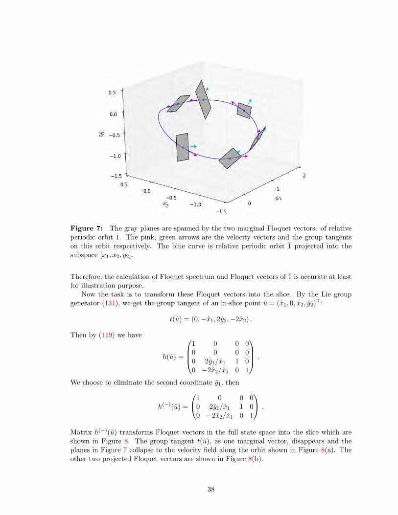
Figure 7: The gray planes are spanned by the two marginal Floquet vectors. of relativeperiodic orbit 1. The pink, green arrows are the velocity vectors and the group tangentson this orbit respectively. The blue curve is relative periodic orbit 1 projected into thesubspace [x1, x2, y2].

Therefore, the calculation of Floquet spectrum and Floquet vectors of 1 is accurate at leastfor illustration purpose.

Now the task is to transform these Floquet vectors into the slice. By the Lie groupgenerator (131), we get the group tangent of an in-slice point u = (x1, 0, x2, y2)>:

t(u) = (0,−x1, 2y2,−2x2) .

Then by (119) we have

h(u) =

1 0 0 00 0 0 00 2y1/x1 1 00 −2x2/x1 0 1

.

We choose to eliminate the second coordinate y1, then

h(−)(u) =

1 0 0 00 2y1/x1 1 00 −2x2/x1 0 1

.

Matrix h(−)(u) transforms Floquet vectors in the full state space into the slice which areshown in Figure 8. The group tangent t(u), as one marginal vector, disappears and theplanes in Figure 7 collapse to the velocity field along the orbit shown in Figure 8(a). Theother two projected Floquet vectors are shown in Figure 8(b).

38

Figure 8: In-slice Floquet vectors for relative periodic orbit 1. The red closed curve is 1.(a) The marginal Floquet vector (pink). (b) The expanding (blue) and contracting (green)Floquet vectors in the slice.

In a similar way [22], Floquet vectors on the slice could be projected onto a Poincaresection. The projection matrix is

hP(u) = 1− |v〉〈∂U |〈v|∂U〉 ,

where U(x) = 0 defines the Poincare section with ∂U its normal direction. v is the in-slicevelocity. A Poincare section can be fixed by choosing three points on it, or equivalently, bythree conditions. Here, we choose a “vertical” Poincare section, namely, we demand thatthe y2 component of its normal direction vanishes. Next, this Poincare section goes throughthe origin (0, 0, 0) and a relative equilibrium

(xe1, xe2, ye2) = (0.439965, −0.386267, 0.070204) ,

shown in Figure 9. In this case, ∂U = (xe2,−xe1, 0) and we get

hP(u) =1

v1xe2 − v2xe1

−v2xe1 v1xe1 0−v2xe2 v1xe2 0−v3xe1 v3xe1 v1xe2 − v2xe1

.

Figure 9 shows the projected expanding and contracting Floquet vectors on the Poincaresection. The marginal vector (velocity field) disappears.

Last, Figure 10 shows the Poincare section and the two projected Floquet vectors. Aset of circularly distributed points around the intersection point evolves for one period andtheir first returning points are recorded. The contracting direction is close to the verticaldirection, and (133) says that the contracting rate is large in this direction. Therefore, thereturning points are squashed heavily in the vertical direction; however, the magnitude ofexpanding multiplier is about 1.5, so the elongation in the horizontal direction is relativelysmall.

In summary, we have reduced the SO(2) symmetry of the two-mode system and discussedthe Floquet vectors of a specific relative periodic orbit in the full state space and in the

39

Figure 9: A vertical Poincare section is constructed from the origin (black point) anda relative equilibrium (blue point) in the slice. The Poincare section intersects 1 (the redclosed curve) at the green point. In-slice Floquet vectors are projected into the Poincaresection. The red/blue vector is the expanding/contracting Floquet vector. The marginalvector along the orbit disappears on the Poincare section.

slice. The marginal direction along the group orbit tangent is eliminated by the slice.Furthermore, we have constructed a Poincare section of codimension two with respect tothe original system. In this Poincare section, the relative periodic orbit 1 is reduced to a fixedpoint with one expanding and one contracting Floquet vector, and the dynamics is greatlysimplified. This simple example illustrates why symmetry reduction is an indispensable toolwhen studying dynamical systems with continuous symmetries.

40

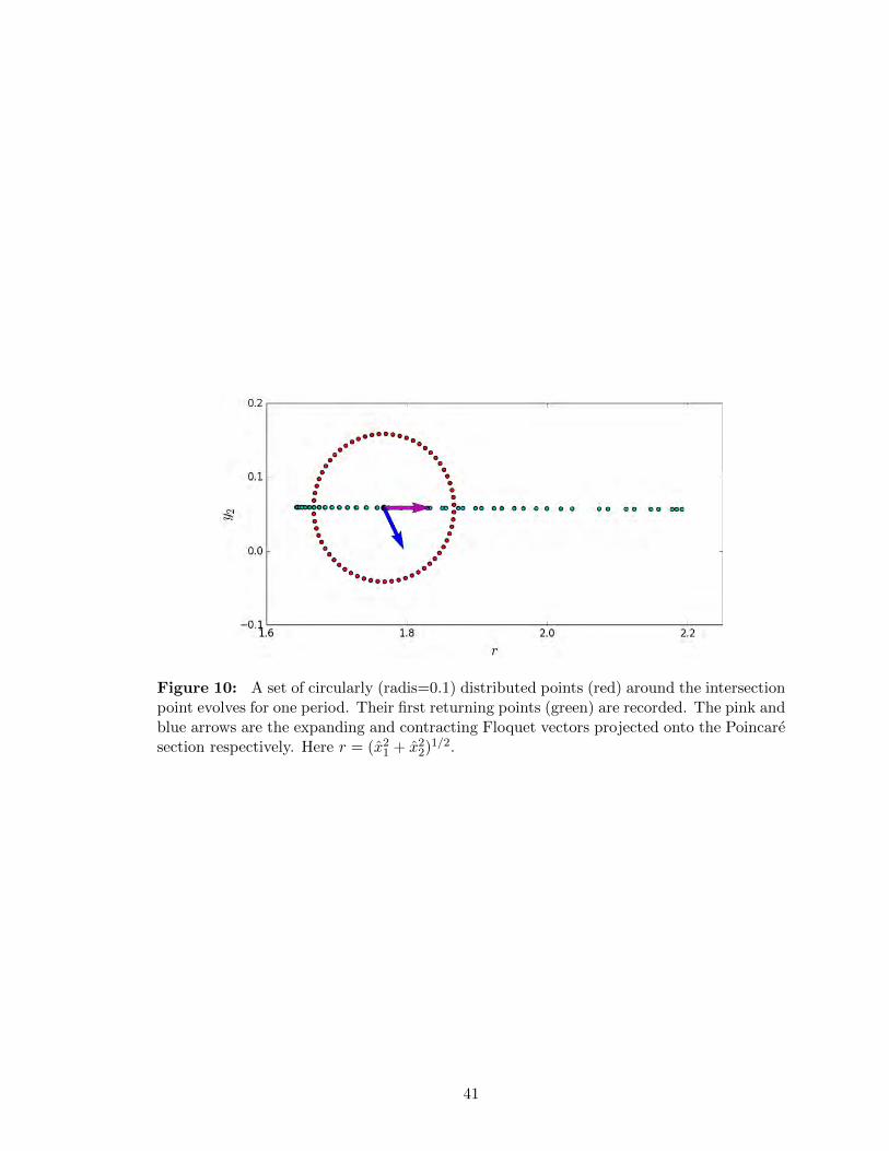
Figure 10: A set of circularly (radis=0.1) distributed points (red) around the intersectionpoint evolves for one period. Their first returning points (green) are recorded. The pink andblue arrows are the expanding and contracting Floquet vectors projected onto the Poincaresection respectively. Here r = (x2

1 + x22)1/2.

41

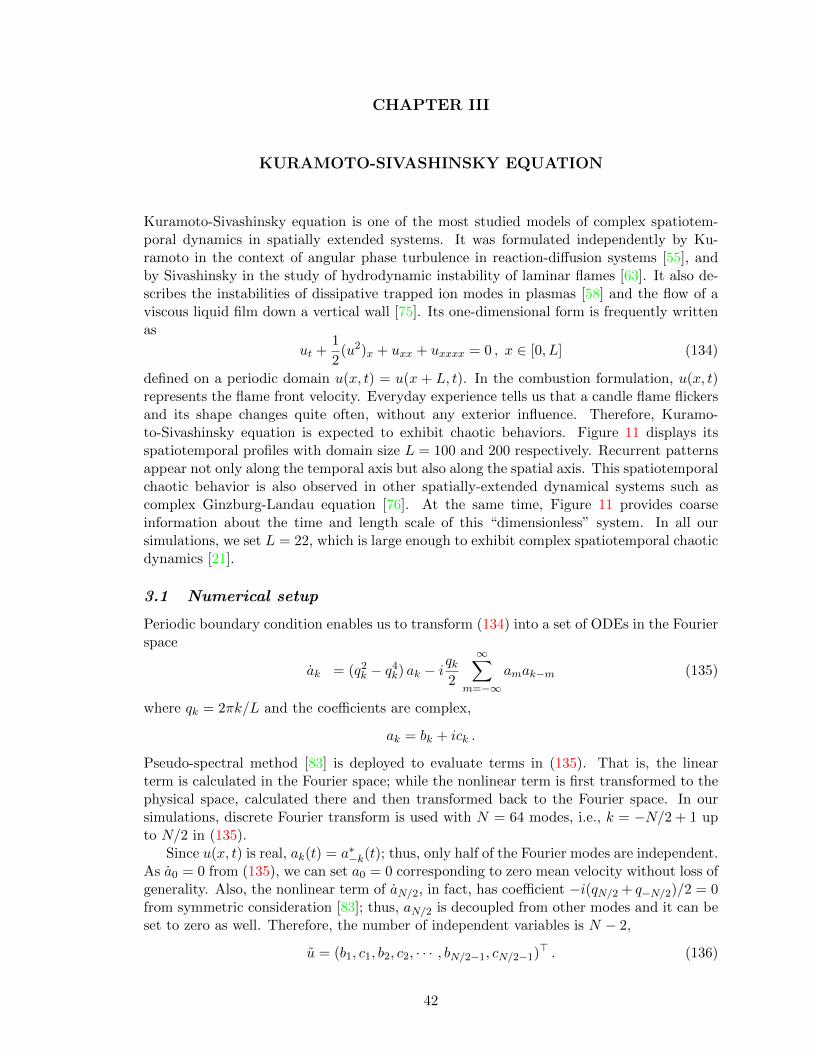
CHAPTER III

KURAMOTO-SIVASHINSKY EQUATION

Kuramoto-Sivashinsky equation is one of the most studied models of complex spatiotem-poral dynamics in spatially extended systems. It was formulated independently by Ku-ramoto in the context of angular phase turbulence in reaction-diffusion systems [55], andby Sivashinsky in the study of hydrodynamic instability of laminar flames [63]. It also de-scribes the instabilities of dissipative trapped ion modes in plasmas [58] and the flow of aviscous liquid film down a vertical wall [75]. Its one-dimensional form is frequently writtenas

ut +1

2(u2)x + uxx + uxxxx = 0 , x ∈ [0, L] (134)

defined on a periodic domain u(x, t) = u(x + L, t). In the combustion formulation, u(x, t)represents the flame front velocity. Everyday experience tells us that a candle flame flickersand its shape changes quite often, without any exterior influence. Therefore, Kuramo-to-Sivashinsky equation is expected to exhibit chaotic behaviors. Figure 11 displays itsspatiotemporal profiles with domain size L = 100 and 200 respectively. Recurrent patternsappear not only along the temporal axis but also along the spatial axis. This spatiotemporalchaotic behavior is also observed in other spatially-extended dynamical systems such ascomplex Ginzburg-Landau equation [76]. At the same time, Figure 11 provides coarseinformation about the time and length scale of this “dimensionless” system. In all oursimulations, we set L = 22, which is large enough to exhibit complex spatiotemporal chaoticdynamics [21].

3.1 Numerical setup

Periodic boundary condition enables us to transform (134) into a set of ODEs in the Fourierspace

ak = (q2k − q4

k) ak − iqk2

∞∑m=−∞

amak−m (135)

where qk = 2πk/L and the coefficients are complex,

ak = bk + ick .

Pseudo-spectral method [83] is deployed to evaluate terms in (135). That is, the linearterm is calculated in the Fourier space; while the nonlinear term is first transformed to thephysical space, calculated there and then transformed back to the Fourier space. In oursimulations, discrete Fourier transform is used with N = 64 modes, i.e., k = −N/2 + 1 upto N/2 in (135).

Since u(x, t) is real, ak(t) = a∗−k(t); thus, only half of the Fourier modes are independent.As a0 = 0 from (135), we can set a0 = 0 corresponding to zero mean velocity without loss ofgenerality. Also, the nonlinear term of aN/2, in fact, has coefficient −i(qN/2 + q−N/2)/2 = 0from symmetric consideration [83]; thus, aN/2 is decoupled from other modes and it can beset to zero as well. Therefore, the number of independent variables is N − 2,

u = (b1, c1, b2, c2, · · · , bN/2−1, cN/2−1)> . (136)

42

Figure 11: Simulations of the one-dimensional Kuramoto-Sivashinsky equation for do-main size L = 100, 200 respectively with random initial conditions. The color representsthe magnitude of u(x, t).

This is the full state space in the discussion that follows.The stiffness caused by the quaternary term in the linear part makes popular integration

methods such as fourth order Runge-Kutta inefficient in this case. Therefore, we resort toexponential integrators [48, 64] to integrate the linear part exactly. In our simulations,exponential time-differencing scheme combined with fourth order Runge-Kutta [19, 52] isimplemented to integrate (135). By this scheme, a relatively large time step can be used toachieve a fourth-order global accuracy.

3.2 Symmetries

The one-dimensional Kuramoto-Sivashinsky equation has three different symmetries. Sup-pose u(x, t) is an orbit in this system, then we have

• Galilean invariance: u(x−ct, t)+c is also a valid orbit, where c is a constant number.These two orbits have different mean velocity

∫dxu.

• Reflection invariance: −u(−x, t) is also a valid orbit. In the Fourier mode space,reflection takes form ak → −a∗k.

• Translation invariance: u(x+ `, t) is another valid orbit. In the Fourier mode space,translation takes form ak → eiqkφak with φ = 2π`/L.

The zeroth Fourier mode a0 represents the mean velocity of u(x, t). by setting a0 = 0 inthe integrator, we eliminate the Galilean symmetry. Therefore, we only need to account forthe O(2) symmetry of this system. Reflection in state space (136) takes the form

R = Diag(−1, 1, −1, 1, · · · ) .

43

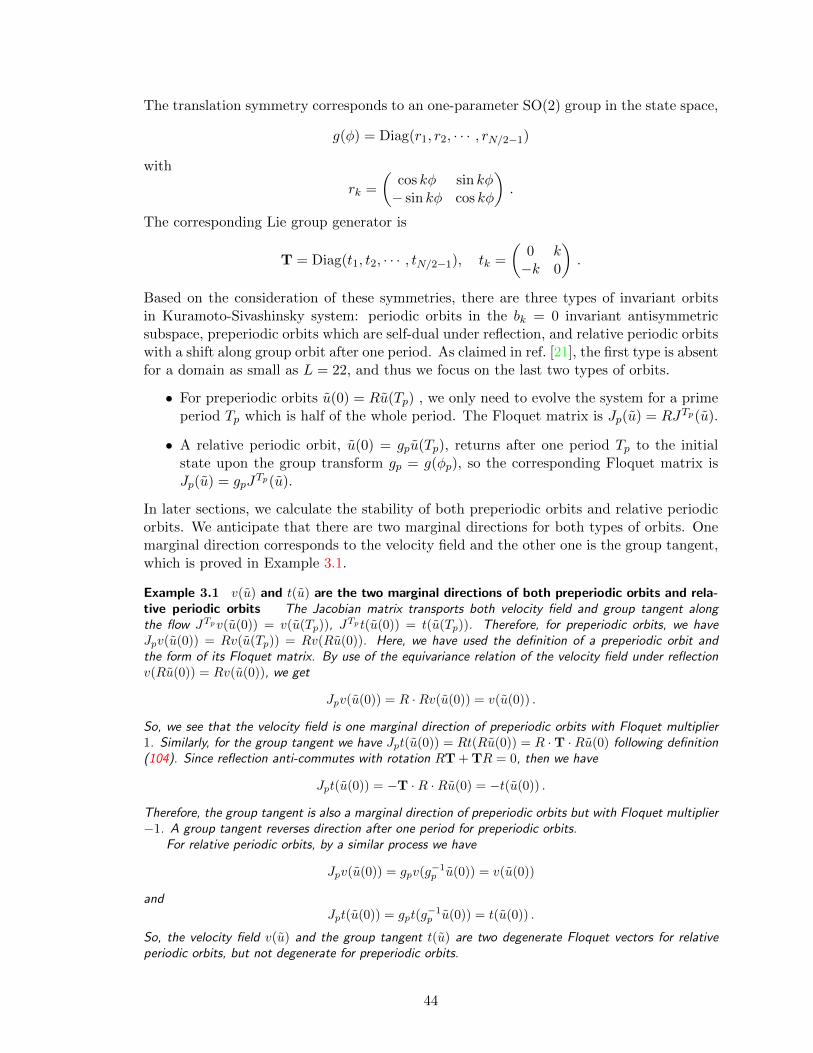
The translation symmetry corresponds to an one-parameter SO(2) group in the state space,

g(φ) = Diag(r1, r2, · · · , rN/2−1)

with

rk =

(cos kφ sin kφ− sin kφ cos kφ

).

The corresponding Lie group generator is

T = Diag(t1, t2, · · · , tN/2−1), tk =

(0 k−k 0

).

Based on the consideration of these symmetries, there are three types of invariant orbitsin Kuramoto-Sivashinsky system: periodic orbits in the bk = 0 invariant antisymmetricsubspace, preperiodic orbits which are self-dual under reflection, and relative periodic orbitswith a shift along group orbit after one period. As claimed in ref. [21], the first type is absentfor a domain as small as L = 22, and thus we focus on the last two types of orbits.

• For preperiodic orbits u(0) = Ru(Tp) , we only need to evolve the system for a primeperiod Tp which is half of the whole period. The Floquet matrix is Jp(u) = RJTp(u).

• A relative periodic orbit, u(0) = gpu(Tp), returns after one period Tp to the initialstate upon the group transform gp = g(φp), so the corresponding Floquet matrix isJp(u) = gpJ

Tp(u).

In later sections, we calculate the stability of both preperiodic orbits and relative periodicorbits. We anticipate that there are two marginal directions for both types of orbits. Onemarginal direction corresponds to the velocity field and the other one is the group tangent,which is proved in Example 3.1.

Example 3.1 v(u) and t(u) are the two marginal directions of both preperiodic orbits and rela-tive periodic orbits The Jacobian matrix transports both velocity field and group tangent alongthe flow JTpv(u(0)) = v(u(Tp)), JTpt(u(0)) = t(u(Tp)). Therefore, for preperiodic orbits, we haveJpv(u(0)) = Rv(u(Tp)) = Rv(Ru(0)). Here, we have used the definition of a preperiodic orbit andthe form of its Floquet matrix. By use of the equivariance relation of the velocity field under reflectionv(Ru(0)) = Rv(u(0)), we get

Jpv(u(0)) = R ·Rv(u(0)) = v(u(0)) .

So, we see that the velocity field is one marginal direction of preperiodic orbits with Floquet multiplier1. Similarly, for the group tangent we have Jpt(u(0)) = Rt(Ru(0)) = R ·T ·Ru(0) following definition(104). Since reflection anti-commutes with rotation RT + TR = 0, then we have

Jpt(u(0)) = −T ·R ·Ru(0) = −t(u(0)) .

Therefore, the group tangent is also a marginal direction of preperiodic orbits but with Floquet multiplier−1. A group tangent reverses direction after one period for preperiodic orbits.

For relative periodic orbits, by a similar process we have

Jpv(u(0)) = gpv(g−1p u(0)) = v(u(0))

andJpt(u(0)) = gpt(g

−1p u(0)) = t(u(0)) .

So, the velocity field v(u) and the group tangent t(u) are two degenerate Floquet vectors for relativeperiodic orbits, but not degenerate for preperiodic orbits.

44

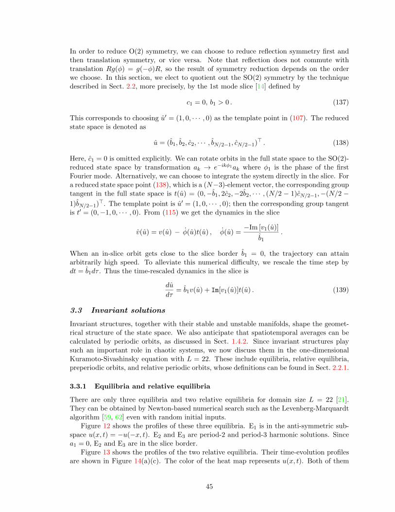
In order to reduce O(2) symmetry, we can choose to reduce reflection symmetry first andthen translation symmetry, or vice versa. Note that reflection does not commute withtranslation Rg(φ) = g(−φ)R, so the result of symmetry reduction depends on the orderwe choose. In this section, we elect to quotient out the SO(2) symmetry by the techniquedescribed in Sect. 2.2, more precisely, by the 1st mode slice [14] defined by

c1 = 0, b1 > 0 . (137)

This corresponds to choosing u′ = (1, 0, · · · , 0) as the template point in (107). The reducedstate space is denoted as

u = (b1, b2, c2, · · · , bN/2−1, cN/2−1)> . (138)

Here, c1 = 0 is omitted explicitly. We can rotate orbits in the full state space to the SO(2)-reduced state space by transformation ak → e−ikφ1ak where φ1 is the phase of the firstFourier mode. Alternatively, we can choose to integrate the system directly in the slice. Fora reduced state space point (138), which is a (N−3)-element vector, the corresponding grouptangent in the full state space is t(u) = (0,−b1, 2c2,−2b2, · · · , (N/2 − 1)cN/2−1,−(N/2 −1)bN/2−1)>. The template point is u′ = (1, 0, · · · , 0); then the corresponding group tangentis t′ = (0,−1, 0, · · · , 0). From (115) we get the dynamics in the slice

v(u) = v(u) − φ(u)t(u) , φ(u) =−Im [v1(u)]

b1.

When an in-slice orbit gets close to the slice border b1 = 0, the trajectory can attainarbitrarily high speed. To alleviate this numerical difficulty, we rescale the time step bydt = b1dτ . Thus the time-rescaled dynamics in the slice is

du

dτ= b1v(u) + Im[v1(u)]t(u) . (139)

3.3 Invariant solutions

Invariant structures, together with their stable and unstable manifolds, shape the geomet-rical structure of the state space. We also anticipate that spatiotemporal averages can becalculated by periodic orbits, as discussed in Sect. 1.4.2. Since invariant structures playsuch an important role in chaotic systems, we now discuss them in the one-dimensionalKuramoto-Sivashinsky equation with L = 22. These include equilibria, relative equilibria,preperiodic orbits, and relative periodic orbits, whose definitions can be found in Sect. 2.2.1.

3.3.1 Equilibria and relative equilibria

There are only three equilibria and two relative equilibria for domain size L = 22 [21].They can be obtained by Newton-based numerical search such as the Levenberg-Marquardtalgorithm [59, 62] even with random initial inputs.

Figure 12 shows the profiles of these three equilibria. E1 is in the anti-symmetric sub-space u(x, t) = −u(−x, t). E2 and E3 are period-2 and period-3 harmonic solutions. Sincea1 = 0, E2 and E3 are in the slice border.

Figure 13 shows the profiles of the two relative equilibria. Their time-evolution profilesare shown in Figure 14(a)(c). The color of the heat map represents u(x, t). Both of them

45

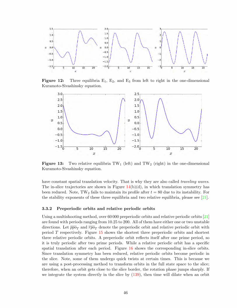
Figure 12: Three equilibria E1, E2, and E3 from left to right in the one-dimensionalKuramoto-Sivashinsky equation.

Figure 13: Two relative equilibria TW1 (left) and TW2 (right) in the one-dimensionalKuramoto-Sivashinsky equation.

have constant spatial translation velocity. That is why they are also called traveling waves.The in-slice trajectories are shown in Figure 14(b)(d), in which translation symmetry hasbeen reduced. Note, TW2 fails to maintain its profile after t = 80 due to its instability. Forthe stability exponents of these three equilibria and two relative equilibria, please see [21].

3.3.2 Preperiodic orbits and relative periodic orbits

Using a multishooting method, over 60 000 preperiodic orbits and relative periodic orbits [21]are found with periods ranging from 10.25 to 200. All of them have either one or two unstabledirections. Let ppoT and rpoT denote the preperiodic orbit and relative periodic orbit withperiod T respectively. Figure 15 shows the shortest three preperiodic orbits and shortestthree relative periodic orbits. A preperiodic orbit reflects itself after one prime period, soit is truly periodic after two prime periods. While a relative periodic orbit has a specificspatial translation after each period. Figure 16 shows the corresponding in-slice orbits.Since translation symmetry has been reduced, relative periodic orbits become periodic inthe slice. Note, some of them undergo quick twists at certain times. This is because weare using a post-processing method to transform orbits in the full state space to the slice;therefore, when an orbit gets close to the slice border, the rotation phase jumps sharply. Ifwe integrate the system directly in the slice by (139), then time will dilate when an orbit

46

(a) (b) (c) (d)

Figure 14: (a)(c) TW1 and TW2 in the full state space. (b)(d) TW1 and TW2 in theslice.

Figure 15: The shortest three preperiodic orbits and three relative periodic orbits in thefull state space. Left three: ppo10.25, ppo14.33 and ppo32.36. Right three: rpo16.31, rpo32.80

and rpo33.50.

gets close to the slice border.This set of preperodic or relative periodic orbits forms the backbone of the global at-

tractor. An ergodic trajectory shadows one orbit for a certain period and then is repelledto the neighborhood of another orbit. This random walk is determined by the stabilityof the preperodic and relative periodic orbits. Table 7 gives the Floquet exponents of thesix orbits in Figure 15, which are obtained by periodic eigendecomposition algorithm thatwill be covered in Chapter 5. There are a few observations. First, all orbits have one ortwo unstable directions and are weakly unstable. ppo14.33 and rpo16.31 are the two mostunstable orbits in our database. Second, all orbits have two marginal directions. For prepe-riodic orbits, one marginal direction has inverse hyperbolicity, i.e., one Floquet multiplieris equal to −1. This was proved in Example 3.1. Third, the leading 8 Floquet exponentsvary sharply among different orbits, but the remaining spectrum is similar. More precisely,for large index k, the real parts of Floquet exponents lie on the curve (q2

k − q4k) as shown

in Figure 17 for ppo10.25. This means that the nonlinear term in (135) is almost negligiblefor higher Fourier modes, and thus they are decoupled from other modes and shrink ex-ponentially with rate |q2

k − q4k|. Also, Floquet exponents appear in pairs for large indices

47

Figure 16: Orbits of Figure 15 in the slice.

Figure 17: The real parts of the Floquet exponents paired for a given k as (k, µ(2k−1))and (k, µ(2k)) for ppo10.25. The dashed line (green) is q2

k − q4k with qk = 2πk/L. The inset

is a magnification of the region containing the 8 leading exponents.

simply because the real and complex part of high Fourier modes have a similar contractionrate. From these observations, we gain an intuition of how many directions are importantin shaping the neighborhood of a pre/relative periodic orbit.

3.4 Floquet vectors

Floquet vectors are important for shaping the geometrical structure of the global attrac-tor in a dissipative system. Floquet vectors of a pre/relative periodic orbit stratify theneighborhood of this orbit. They give a rough picture of the dynamics close to this or-bit. On the other hand, the stable and unstable manifolds of this orbit are tangent tothe Floquet vectors, so numerically we grow the unstable manifolds from unstable Floquetvectors. Thus, Floquet vectors provide a way of studying the dynamics far away from thisorbit. Calculating Floquet vectors is not an easy task due to the large range of orders ofexpansion/contraction rates indicated by Table 7. However, with the invention of periodic

48

Table 7: The first 10 and last four Floquet multipliers Λi = exp(T µ(i) ± iθi) for sixrepresentative orbits. θi column lists either the phase, if the Floquet multiplier is complex,or ‘-1’ if the multiplier is real, but inverse hyperbolic.

ppo10.25 ppo14.33 ppo32.36

i µ(i) θi i µ(i) θi i µ(i) θi1,2 0.033209 ±2.0079 1 0.31095 -1 1,2 0.064755 ±1.97903 -4.1096e-13 2 -1.7825e-12 3 -6.3772e-144 -3.3524e-14 -1 3 2.5049e-13 -1 4 1.9306e-13 -15 -0.21637 4 -0.12154 -1 5 -0.175116,7 -0.26524 ±2.6205 5 -0.20150 6 -0.24418 18 -0.33073 -1 6 -0.29265 -1 7,8 -0.27968 ±0.69909 -1.9605 7,8 -0.34313 ±1.7872 9 -1.9868 -110 -1.9676 -1 9 -1.9530 -1 10 -1.9891

10 -1.9928· · · · · · · · ·

59 -5313.6 -1 59 -5312.7 -1 59 -5313.3 -160 -5317.6 60 -5318.4 60 -5317.961 -6051.8 -1 61 -6057.8 61 -6052.962 -6080.4 62 -6074.4 -1 62 -6079.2 -1

rpo16.31 rpo32.80 rpo33.50

i µ(i) θi i µ(i) θi i µ(i) θi1 0.32791 1,2 0.018610 ±1.397964 1 0.0730492 2.8679e-12 3 6.1717e-14 2 0.015160 -13 2.3559e-13 4 -5.7430e-14 3 1.1725e-144 -0.13214 -1 5 -0.19688 -1 4 -8.8541e-145,6 -0.28597 ±2.7724 6 -0.24726 -1 5 -0.11390 -17 -0.32821 -1 7,8 -0.30869 ±2.20628 6 -0.252248 -0.36241 9 -1.9660 -1 7,8 -0.26398 ±1.05219,10 -1.9617 ±2.2411 10 -1.9575 -1 9,10 -1.993196 ±0.60493

· · · · · · · · ·59 -5314.4 59 -5313.9 59 -5313.2 -160 -5317.7 60 -5317.2 60 -5318.0 -161 -6059.2 61 -6053.9 -1 61 -6052.562 -6072.9 62 -6078.3 -1 62 -6079.7

eigendecomposition algorithm (Chapter 5), we are able to get a full set of Floquet vectorsat each point of a pre/relative periodic orbit.

Figure 18 shows the real part of the 1st Floquet vector, the 5th, the 10th and 30thFloquet vectors of ppo10.25. As index increases, Floquet vectors behave more like pureFourier modes. Figure 19 shows a few selected Floquet vectors along ppo10.25 and rpo16.13 forone prime period respectively. We can see that the spatiotemporal plots of the few leadingFv s, see panels (a,b) and (e,f), exhibit turbulent structures containing only long waves,for both ppo10.25 and rpo16.13, but for Floquet vectors corresponding to strong contractionrates, i.e., panels (c,d), (g,h), the configurations are almost pure sinusoidal curves. Thepower spectra in Figure 20 demonstrate this point too. The leading 8 Floquet vectors havelarge components in the first 5 Fourier modes and the spectra are entangled with each

49

(a) (b)

(c) (d)

Figure 18: Floquet vectors of ppo10.25 at t = 0 in Figure 15. (a) is the real part of the1st Floquet vector. (b), (c) and (d) are the 5th, 10th, and 30th Floquet vectors.

other; while the remaining Floquet vectors almost concentrate on a single Fourier modeand are decoupled from each other; more specifically, the ith Floquet vector with i ≥ 9peaks at the d i2eth1 mode in Figure 20. Takeuchi et al. [79, 90] observe similar features incovariant vectors along ergodic trajectories and by measuring the tangency between thesetwo groups of covariant vectors, they reach a reasonable conclusion about the dimensionof the inertial manifold in Kuramoto-Sivashinsky equation and complex Ginzburg-Landauequation. Therefore, we anticipate that analyzing the tangency of Floquet vectors alongdifferent pre/relative periodic orbits can also lead to the same conclusion, which will bediscussed in detail in Chapter 4.

3.5 Unstable manifolds and shadowing

Unstable manifolds of the three equilibria and the two relative equilibria, and their con-necting orbits in the full state space have been discussed in detail in [21]. With the advancein the technique of symmetry reduction, we have a better picture of the in-slice state space.Moreover, relative periodic orbits become periodic in the slice, which helps us organize the

1 Here, dxe denotes the smallest integer no less than x.

50

(a) (b) (c) (d) (e) (f) (g) (h)

Figure 19: (a) ∼ (d) : the 1st (real part), 5th, 10th and 30th Floquet vector alongppo10.25 for one prime period. (e) ∼ (h) : the 1st, 4th (real part), 10th (imaginary part)30th (imaginary part) Floquet vector along rpo16.31 for one prime period. Axes and colorscale are the same as Figure 15.

pre/relative periodic orbits in our database. In this section, we will discuss the unstablemanifolds of (relative) equilibria and show shadowing incidences of different orbits.

3.5.1 O(2) symmetry reduction

Sect. 3.2 introduces the 1st mode slice to reduce SO(2) in the one-dimensional Kuramoto-Sivashinsky equation. Here, we go one step further, i.e., quotienting out reflection symmetryin the 1st mode slice. Different from the invariant polynomial approach used by N. B.Budanur [11, 12], we turn to the fundamental domain.

In Sect. 3.2, the 1st mode slice (137) is defined as the half hyperplane c1 = 0, i.e., theimaginary part of the 1st mode vanishes. Here, when reducing reflection in the slice, wefind it is more convenient to define the slice as

b1 = 0, c1 > 0 , (140)

namely, we let the real part of the 1st mode vanish. Literature [14, 27] all chooses (137).That is why we insist on using (137) to define the 1st mode slice in other chapters of thisthesis. Thus conversion (140) is only used in this section. The benefit of using (140) insteadof (137) in this section is that the reflection axis is parallel to the slice (140) such that thereflection rule does not change from the full state space to the slice.

Example 3.2 Reflection rule is invariant under SO(2) reduction by (140) Suppose two statesu1 and u2 in the full state space are related to each other by reflection, u2 = Ru1. Let u1 and u2 betheir reduced states in the slice (140). If the 1st Fourier mode of u1 is (b1 + ic1), then the 1st Fouriermode of u2 is (−b1 + ic1). So if g(φ1) transforms u1 onto the positive imaginary axis in (b1, c1) plane,that is, u1 = g(φ1)u1, then u2 = g(−φ1)u2 as shown in Figure 21. Therefore,

u2 = g(−φ1)Ru1 = Rg(φ1)u1 = Ru1 .

Here we have used the anti-commuting relation g(−φ)R = Rg(φ). So we see that the choice of slice(140) keeps the reflection rule unchanged.

The reflection operator is R = Diag(−1, 1, −1, 1, · · · ). Since b1 = 0 in the slice, thus bkwith k > 1 changes sign after reflection. We define the fundamental domain in the slice as

b2 > 0 . (141)

51

(a) (b)

Figure 20: The power spectrum of the first 30 Floquet vectors for ppo10.25 (left) andrpo16.31 (right) at t = 0. Red lines correspond to the leading 8 Floquet vectors; while theblue lines correspond to the left 22 Floquet vectors with the ith one localized at index d i2e.Power at index k is defined to be the square of the kth Fourier coefficient’s magnitude ofFloquet vectors. The x-axis is labeled by the Fourier mode indices. Only the k > 0 part isshown, and the part for negative k follows by reflection. For complex Floquet vectors, thepower spectra of the real part and imaginary part are calculated separately. Since almostall contracting Floquet vectors of rpo16.31 form complex conjugate pairs, their power peaksare far less than 1, as shown in panel (b).

Whenever an in-slice orbit leaves the fundamental domain, we transform it back by reflec-tion. With the sacrifice of allowing discontinuity, we quotient out O(2) symmetry in theone-dimensional Kuramoto-Sivashinsky equation.

3.5.2 Unstable manifold of E2

There are three equilibria E1, E2 and E3 and two relative equilibria TW1 and TW2 in thissystem. E2 and E3 are symmetric under shifts by L/2 and L/3 respectively as shown inFigure 12. As shown in [21], one branch of the unstable manifold of E1 and the unstablemanifold of E3 terminate at E2 or its symmetry-equivalent counterparts in the full statespace. Also, the unstable manifold of E2 is a set of homoclinic orbits of itself. Therefore,we believe that E2 has a large influence on the geometrical structure of the in-slice statespace.

Figure 22 shows the unstable manifold of E2 and several pre/relative periodic orbits inthe fundamental domain projected into some Fourier mode subspace. Since E2 and E3 arein the slice border, their SO(2) symmetry can not be quotiented out by the 1st mode slice.The blue and green straight lines are the group orbits of E2 and E3 in the slice respectively.These two lines depict the slice border in this three-dimensional subspace. Note, this doesnot mean that the unstable manifold of E2 should also live in the slice. Actually, E2

has one pair of unstable complex conjugate stability eigenvectors, which do have nonzerofirst Fourier mode components. Hence, the corresponding unstable manifolds have uniquelocations, determined by the first Fourier mode phase of this pair of eigenvectors, in thesymmetry reduced state space.

There are a few interesting observations in Figure 22. First, the pre/relative periodic

52

b1

c1u2 u1

φ1−φ1

Figure 21: Illustration of the phase relation in Example 3.2.

orbits look continuous, but in fact, they are discontinuous in the fundamental domain. Wechoose the three-dimensional subspace to be (c1, c3, c2) which is invariant under reflection.Thus reflection has no effect on this specific projection. Second, the unstable manifold ofE2 is discontinuous. Whenever it crosses the slice border, there is a phase jump by π, whichcauses c3 to change sign. Third, we can see that both ppo8 (ppo41.08) and rpo3 (rpo33.50)shadow the unstable manifold of E2 for a certain period of time. Actually, there are plentyof pre/relative periodic orbits in our database that shadow the unstable manifold of E2. Inthis sense, E2 plays a substantial role in shaping the dynamics.

3.5.3 Shadowing among orbits

In Figure 22, we see that ppo2 (ppo14.33) is quite similar to rpo1 (rpo16.31). Actually, thesetwo orbits shadow each other and have similar periods. There are a lot of other shadowingincidences between different pre/relative periodic orbits. For example, in Figure 23(a),rpo57.59 shadows rpo16.31 and rpo35.97 closely. The period of this longer orbit is close to thesum of the periods of the two shorter orbits. In Figure 23(b), ppo57.67 shadows ppo14.33 fora certain period of time. Shadowing helps us classify all the pre/relative periodic orbitsand helps build the symbolic dynamics of this system. This is important for the spectraldeterminant (73) to converge quickly when it is expanded by only a few short orbits [22].

On the other hand, preperiodic orbits and relative periodic orbits frequently show up inpairs in the one-dimensional Kuramoto-Sivashinsky equation. For instance, rpo57.59 in Fig-ure 23(a) and ppo57.67 in Figure 23(b) are such a pair. N. B. Budanur and P. Cvitanovic [12]believe that this phenomenon comes from symmetry-breaking bifurcation as the domain sizeL is varied.

53

(a)

(b)

Figure 22: The unstable manifold of E2 in the fundamental domain in the slice. Thedense set of thin curves is the unstable manifold of E2. The blue and green straight lines arethe group orbits of E2 and E3 respectively. ppo2 is ppo14.33 in Figure 15. rpo1 is rpo16.31.ppo8 is ppo41.08. rpo3 is rpo33.50. Projection axes are the imaginary parts of the first 3Fourier modes [v1, v2, v3] = [c1, c3, c2]. This set is invariant under reflection.

54

(a)

(b)

Figure 23: Shadowing among pre/relative periodic orbits in the fundamental domain.The dense set of thin curves is the unstable manifold of E2. The two straight lines are thegroup orbits of E2 and E3 respectively. Projection axes are the imaginary parts of the first3 Fourier modes [v1, v2, v3] = [c1, c3, c2]. This set is invariant under reflection. (a) The threerelative periodic orbits are (red) rpo16.31, (blue) rpo35.97 and (black) rpo57.59. (b) The redpreperiodic orbit is ppo2 (ppo14.33). The black preperiodic orbit is ppo24 (ppo57.67).

55

CHAPTER IV

THE INERTIAL MANIFOLD OF A KURAMOTO-SIVASHINSKYSYSTEM

As stated in Sect. 1.2, dynamics in chaotic dissipative systems is expected to land, aftera transient period of evolution, on the inertial manifold [18, 34, 70, 80, 81], which is afinite-dimensional object in state space. This is true even for infinite-dimensional systemsdescribed by partial differential equations, and offers hope that their asymptotic dynamicsmay be represented by a finite set of ordinary differential equations.

The existence of a finite-dimensional inertial manifold has been established for systemssuch as the Kuramoto-Sivashinsky, the complex Ginzburg-Landau, and some reaction-diffusion systems [81]. For the Navier-Stokes flows its existence remains an open prob-lem [80], but dynamical studies, such as the determination of sets of periodic orbits em-bedded in turbulent flows [40, 86], strengthen the case for a geometrical description ofturbulence.

In this chapter, we discuss the existence and the dimension of the global attractorand the inertial manifold for a particular one-dimensional Kuramoto-Sivashinsky system,defined on a “minimal domain”. Our discussion has two parts. In Sect. 4.1, we review themathematical proof of the existence of a global attractor and the rigorous bounds for thedimension of the inertial manifold. In Sect. 4.2, we determine the dimension of the inertialmanifold by the numerical study of Floquet vectors along pre/relative periodic orbits forthis particular system.

4.1 The existence of an inertial manifold

As discussed in Sect. 1.2.3, an inertial manifold is the graph of a map Φ : PnM 7→ QnM,where Pn is the projection to the eigenspace spanned by the eigenvectors of ∂xx + ∂xxxx,corresponding to its smallest n eigenvalues. ∂xx + ∂xxxx has eigenvalues −q2

k + q4k with

Fourier modes as eigenvectors. Thus the existence of an inertial manifold indicates thata finite number of low frequency Fourier modes can describe the asymptotic behavior ofthis system. Any trajectory will be attracted to this manifold exponentially fast. Thisexpectation is also reflected in (135), where the velocity field of a high frequency Fouriermode, i.e., ak with large k, is dominated by the linear part (q2

k−q4k) ak. Thus, high frequency

Fourier modes are almost decoupled from other modes.An inertial manifold exists in a system which possesses the strong squeezing property

(22)–(25). As shown in Theorem 1.7, as long as the spectrum of ∂xx+∂xxxx has a sufficientlylarge gap for some n, then an inertial manifold exists. The kth eigenvalue of ∂xx + ∂xxxx isλk = −q2

k+q4k. so λn+1−λn is unboundedly increasing with respect to n. In one-dimensional

Kuramoto-Sivashinsky equation (134), the nonlinear part of the velocity field is −uux. Ifwe can determine a Lipschitz constant C1 for −uux, then surely there is an n such thatλn+1 − λn > 4C1. As a result, an inertial manifold exists.

Strong squeezing property has been shown to hold for one-dimensional Kuramoto-Siva-shinsky equation (Theorems 3.2 and corollary 3.7 in [35], Theorem 4 in [69]). Moreover,

56

Robinson (Corollary 5 in [69]) states that if there is an absorbing ball with radius O(Lα) 1 inthe one-dimensional Kuramoto-Sivashinsky equation, then an inertial manifold exists withdimension bounded above by O(L3α/5+3/2). Also, Theorem 1.3 says that a global attractorexists if an absorbing set exists in the state space. Therefore, both a global attractor andan inertial manifold exist, provided the existence of an absorbing set in the state space,which is a Hilbert space with the L2 norm

‖u ‖2 =

(∫ L

0u2dx

)1/2

.

4.1.1 Rigorous upper bounds

In 1985, Nicolaenko, Scheurer and Temam [65] gave the first asymptotic boundedness of theL2 norm of u(x, t) in the antisymmetric subspace, showing the existence of an absorbingball S = {u : ‖u ‖2 ≤ CL5/2} for antisymmetric solutions. They also show that the Haus-dorff dimension of the global attractor is bounded above by O(L13/8). This antisymmetricassumption was later removed by Goodman [43]. The estimate was improved by Collet etal. [17] who extended it to the whole state space and improved the exponent from 5/2 to8/5. In 2006, Bronski and Gammbill [10] gave a better upper bound

lim supt→∞

‖u ‖2 = O(L32 ) . (142)

All these results were obtained through the Lyapunov function approach, the main idea ofwhich is to find an appropriate gauge function Φ(x):

u(x, t) = v(x, t) + Φ(x) (143)

such that the transformed field ‖ v(x, t) ‖2 is bounded. Upper bound (142) is claimed tobe the best result one can get by the Lyapunov function approach. On the other hand, bytreating Kuramoto-Sivashinsky equation as a perturbation of Burgers’ equation, Giacomelliand Otto [39] proved that 2

lim supt→∞

||u||2 = o(L32 ) . (144)

Later on, Otto [67] shows that

lim supt→∞

1

T

∫ T

0dt ‖ |∂x|αu ‖2 = O(L · ln10/3 L) , 1/3 < α ≤ 2 ,

and claims that it is the optimal bound for the one-dimensional Kuramoto-Sivashinskyequation. The norm of the time-averaged fractional derivatives of u(x, t) is almost propor-tional to L1/2. Bronski and Gammbill [10] also claim that 1/2 is believed to be the bestpossible exponent.

Based on an upper bound of size of the attracting set, we can estimate the dimensionof the inertial manifold. In 1988, Foias, Nicolaenko, Sell and Temam [35] gave an upperbound O(L7/2) for the dimension of the inertial manifold. Better estimate O(L2.46) is

1 The big-O notation: f(x) = O(g(x)) if and only if there exists a positive real number M and a realnumber x0 such that |f(x)| ≤M |g(x)| for all x ≥ x0.

2 The little-O notation : f(x) = o(g(x)) if and only if there exists a a real number x0 such that |f(x)| ≤M |g(x)| for all x ≥ x0 and for all positive real number M .

57

given in ref. [33, 50]. Based on bound (144), the upper bound can be further improved too(L12/5) [39].

In the remaining part of this section, we show the existence of an absorbing ball throughthe Lyapunov function approach. The main result comes from the work of Collet et al. [17].Though the estimate is not optimal, it demonstrates the general process of obtaining theupper bound by choosing an appropriate gauge function in (143).

4.1.2 Existence of an absorbing ball

Due to Galilean invariance of the Kuramoto-Sivashinsky equation, we impose zero meanvelocity

∫ L0 u(x, t)dx = 0 in the state space. Then we state that

Theorem 4.1 There is an absorbing ball S with radius CL8/5 in the one-dimensional Ku-ramoto-Sivashinsky equation defined on a periodic domain [0, L]. Here, C is a constant.

Here, for simplicity, we only provide the proof of theorem 4.1 for the antisymmetric case.For the full proof, please refer [17, 50]. That is , we impose that both v(x, t) and Φ(x) in(143) have period L and are antisymmetric: v(−x, t) = −v(x, t), Φ(−x) = −Φ(x). Thenrewriting Kuramoto-Sivashinsky equation (134) in terms of v(x, t), we have

vt = (−∂2x − ∂4

x)(v + Φ)− vvx − vΦx − Φvx − ΦΦx .

Multiplying on both sides of the above equation with v and integrating over the wholedomain, we get

1

2∂t

∫v2 =

∫v(−∂2

x − ∂4x)(v + Φ)−

∫v2vx −

∫v2Φx −

∫vΦvx −

∫vΦΦx

=

∫v(−∂2

x − ∂4x)(v + Φ)− 0−

∫v2Φx +

1

2

∫v2Φx −

∫vΦΦx

=

∫v(−∂2

x − ∂4x)(v + Φ)− 1

2

∫v2Φx −

∫vΦΦx . (145)

In the above,∫v2vx vanishes because of the periodic boundary condition. From (145), we

see that the evolution of ‖ v(x, t) ‖22 depends on the choice of the gauge function. In orderto bound ‖ v(x, t) ‖2, we need to bound the right side of (145) for some carefully chosengauge function Φ(x). Before that, we define notation

(v1, v2)γΦ =

∫v1(∂2

x + ∂4x + γΦx)v2 . (146)

Therefore, (145) becomes

1

2∂t

∫v2 = −(v, v)Φ/2 − (v,Φ)Φ . (147)

To bound the right side of (147), we bring up two propositions.

Proposition 4.2 There is a constant K and an antisymmetric gauge function Φ(x) suchthat for all γ ∈ [1

4 , 1] and all antisymmetric v(x, t) one have inequalities

(v, v)γΦ ≥1

4

∫(v2xx + v2) and (148)

(Φ,Φ)γΦ ≤ KL16/5 . (149)

58

Proposition 4.3 Definition (146) defines an inner product in the L2 space.

With these two propositions, we then continue from (147),

1

2∂t

∫v2 ≤ −(v, v)Φ/2 + (v, v)

1/2Φ (Φ,Φ)

1/2Φ (150)

= −(v, v)Φ/2 + (ε(v, v)Φ)1/2

(1

ε(Φ,Φ)Φ

)1/2

≤ −(v, v)Φ/2 +ε

2(v, v)Φ +

1

2ε(Φ,Φ)Φ

= −∫v

((1− ε

2)(∂2

x + ∂4x) + (

1

2− ε

2)γΦx

)v +

1

2ε(Φ,Φ)Φ

= −(1− ε

2)(v, v)Φ( 1

2− ε

2)/(1− ε

2) +

1

2ε(Φ,Φ)Φ

≤ −(1− ε

2)1

4

∫(v2xx + v2) +

1

2ε(Φ,Φ)Φ (151)

≤ −(1− ε

2)1

4

∫v2 +

1

2ε(Φ,Φ)Φ .

We set ε = 2/3 to make (12 − ε

2)/(1− ε2) = 1/4, so we get

∂t

∫v2 ≤ −1

3

∫v2 +

3

2(Φ,Φ)Φ . (152)

Step (150) has used proposition 4.3 such that Cauchy-Schwarz inequality can be applied: (v,Φ)2 ≤ (v, v)(Φ,Φ). Step (151) has used (148) in proposition 4.2. Derivative of

∫v2

is bounded as shown in (152) and note that term 34(Φ,Φ)Φ does not depend on time, so

applying lemma 1.5, we obtain∫v(x, t)2dx ≤ e−t/3

∫v(x, 0)2dx+

9

2(1− et/3)(Φ,Φ)Φ . (153)

Since u(x, t) = v(x, t) + Φ(x), we therefore obtained an absorbing ball in the Kuramoto-Sivashinsky equation centered at Φ(x) with radius ρ > ρ0, where

ρ0 = 3

√(Φ,Φ)Φ

2= O(L8/5) . (154)

Here, we have used relation (149). Actually, Jolly, Rosa, and Temam [50] constructed agauge function such that the L2 norm of Φ is bounded ‖Φ ‖2 = O(L3/2). Therefore, thecenter of the absorbing ball can be moved to the origin. Thus

lim supt→∞

‖u(x, t) ‖2 = O(L8/5) +O(L3/2) = O(L8/5) .

As shown in (154), the radius of the absorbing ball depends on the choice of the gaugefunction Φ(x). To make the radius as small as possible, we try to minimize the exponent in(149) and at the same time to meet the requirement of (148). This requires us to choose thegauge function with the least norm which also supports (149) and proposition 4.3. Actually,proposition 4.3 is a natural corollary of proposition 4.2. The reason is as follows. Apparently,the bilinear form (146) satisfies relations (λv1 + µv2, v3)γΦ = λ(v1, v3)γΦ + µ(v2, v3)γΦ and(v1, v2)γΦ = (v2, v1)γΦ. In order to make it an inner product, we only need to demonstratethat (v, v)γΦ ≥ 0 with equality if and only if v = 0. Equation (148) provides this relation.Therefore, we only need to prove proposition 4.2, which is given in appendix B.

59

4.2 Numerical evidence provided by Floquet vectors

While mathematical approaches provide rigorous bounds on dimensions of inertial mani-folds, their constructive description remains a challenge. In this section, we provide numer-ical evidence that gives a specific integer dimension of the inertial manifold inside the one-dimensional Kuramoto-Sivashinsky equation. We show that the finite-dimensional physicalmanifold can be precisely embedded in its infinite-dimensional state space, thus opening apath towards its explicit construction. The key idea [22] is to populate the inertial man-ifold by an infinite hierarchy of unstable time-invariant solutions, such as periodic orbits,an invariant skeleton which, together with the local “tiles” obtained by linearization of thedynamics, fleshes out the physical manifold. Chaos can then be viewed as a walk on theinertial manifold, chaperoned by the nearby unstable solutions embedded in the physicalmanifold. Unstable periodic orbits have already been used to compute global averages ofspatiotemporally chaotic flows [16, 21, 40, 56].

In our analysis, we use 200 preperiodic orbits and 200 relative periodic orbits. Theseare the shortest periodic orbits taken from the set of over 60 000 determined in ref. [21]by near-recurrence searches. The method preferentially finds orbits embedded in the long-time attracting set but offers no guarantee that all orbits up to a given period have beenfound. There are infinitely many unstable orbits, and each of them possesses infinitelymany Floquet modes. While in the example that we study here we do not have a detailedunderstanding of the organization of periodic orbits (their symbolic dynamics), we showthat one only needs to consider a finite number of them to tile the physical manifold to areasonable accuracy. We also show, for the first time, that each local tangent tile spannedby the Floquet vectors of an unstable periodic orbit splits into a set of physical Floquetmodes and the remaining set of spurious modes. Furthermore, we verify numerically thatthe physical Floquet manifold coincides locally with the physical manifold determined bythe covariant Lyapunov vectors approach.

4.2.1 Motivation from covariant vectors

Recent progress towards this aim came from numerical investigations of the covariant vectorsof spatiotemporally chaotic flows [79, 90], made possible by the algorithms developed inrefs. [41, 42, 87]. These works have revealed that the tangent space of a generic spatially-extended dissipative system is split into two hyperbolically decoupled subspaces: a finite-dimensional subspace of “entangled” or “physical” Lyapunov modes (referred to in whatfollows as the “physical manifold”), which is presumed to capture all long-time dynamics,and the remaining infinity of transient (“isolated,” “spurious”) Lyapunov modes. Covariant(Lyapunov) vectors span the Oseledec subspaces [28, 66] and thus indicate the intrinsicdirections of growth or contraction at every point on the physical manifold. The dynamicsof the vectors that span the physical manifold is entangled, with frequent tangencies betweenthem. The spurious modes, on the other hand, are damped so strongly that they are isolated- at no time do they couple by tangencies to the physical modes. Specifically, for domainsize L = 22, the physical manifold consists of the leading 8 covariant vectors.

It was conjectured in ref. [79, 90] that the physical manifold provides a local linear ap-proximation to the inertial manifold at any point on the attractor, and that the dimensionof the inertial manifold is given by the number of the physical Lyapunov modes. Furthersupport for this conjecture was provided by ref. [89], which verified that the vectors con-necting pairs of recurrent points –points on the chaotic trajectory far apart in time but

60

nearby each other in state space– are confined within the local tangent space of the physicalmanifold.

While these works showed that the physical manifold captures the finite dimensionalityof the inertial manifold, they do not tell us much about how this inertial manifold is ac-tually laid out in state space. This is the primary reason that we instead study the set ofpre/relative periodic orbits inside this system as they form the backbone the attractor.

4.2.2 Decoupling of local Floquet exponents

j

λ j

t0 Tp

λ j(x

(t))

-10

-5

0

t0 Tp

-1

-0.5

0

0.5

(a)

(b) (c)

j = 9, 10

j = 11, 12

j = 13, 14

j = 1,2j = 3j = 4

j = 5j = 6,7j = 8

0 5 10 15 20-40

-30

-20

-10

0

0 2 4 6 8-0.4

-0.2

0

0.2

0.4

ppo10.25

rpo16.31

chaotic

Figure 24: (a) Floquet exponents for ppo10.25 (circles), rpo16.31 (squares), and Lyapunovexponents of a chaotic trajectory (crosses). The inset shows a close-up of the 8 leadingexponents. For the full Floquet spectrum of these two orbits, see Table 7. (b) Timeseries of local Floquet exponents λj(u(t)) for ppo10.25. (c) Close-up of (b) showing the8 leading exponents. Dashed lines indicate degenerate exponent pairs corresponding tocomplex Floquet multipliers.

The definitions of Floquet exponents and Floquet vectors are given in Sect. 1.3.1. Morespecifically, for preperiodic orbits and relative periodic orbits defined in Sect. 3.2, Floquetmultipliers Λj and vectors ej(u) are the eigenvalues and eigenvectors of Jacobian matrixJp = RJTp or Jp = g(θp)J

Tp for pre-periodic or relative periodic orbits, respectively, ex-plained in Sect. 3.2. The Floquet exponents λj (if complex, we shall only consider theirreal parts, with multiplicity 2) are related to multipliers by λj = ln |Λj |/Tp. For an orbit(λj , ej) denotes the jth Floquet (exponent, vector); for a chaotic trajectory it denotes thejth Lyapunov (exponent, vector).

61

Figure 24 (a) shows the Floquet exponents spectra for the two shortest orbits, ppo10.25

and rpo16.31, overlaid on the Lyapunov exponents computed from a chaotic trajectory. Thebasic structure of this spectrum is shared by all 400 orbits used in our study. 3 Forchaotic trajectories, hyperbolicity between an arbitrary pair of Lyapunov modes can becharacterized by a property called the domination of Oseledec splitting (DOS) [7, 68].Consider a set of finite-time Lyapunov exponents

λτj (u) ≡ 1

τln ||Jτ (u)ej(u)|| , (155)

with L2 normalization ‖ ej(u) ‖ = 1. A pair of modes j < ` is said to fulfill ‘DOS strictordering’ if λτj (u) > λτ` (u) along the entire chaotic trajectory, for τ larger than some lowerbound τ0. Then this pair is guaranteed not to have tangencies [7, 68]. For chaotic trajecto-ries, DOS turned out to be a useful tool to distinguish physical modes from hyperbolicallydecoupled spurious modes [79, 90]. Periodic orbits are by definition the infinite-time orbits(τ can be any repeat of Tp), so generically all nondegenerate pairs of modes fulfill DOS.Instead, we find it useful to define, by analogy to the ‘local Lyapunov exponent’ [9], the‘local Floquet exponent’ as the action of the strain rate tensor [57] 2D(u) = A(u)> +A(u)(where A is the stability matrix (28)) on the normalized jth Floquet eigenvector,

λj(u) = ej(u)>D(u) ej(u) = limτ→0

λτj (u) . (156)

We find that time series of local Floquet exponents λj(u(t)) indicate a decoupling of theleading ‘physical’ modes from the rest of the strictly ordered, strongly negative exponents[Figure 24 (b) and (c)]. Another example, the local Floquet exponents of rpo16.31 is shownin Figure 25. Perhaps surprisingly, for every one of the 400 orbits we analyzed, the numberof the physical Floquet modes was always 8, equal to the previously reported number of thephysical Lyapunov modes for this system [89]. 4 This leads to our first surmise: (1) eachindividual orbit embedded in the attracting set carries enough information to determine thedimension of the physical manifold.

4.2.3 Decoupling of Floquet vectors

For an infinite-time chaotic trajectory, hyperbolicity can be assessed by measuring thedistribution of minimal principal angles [6, 53] between any pair of subspaces spanned byLyapunov vectors [41, 79, 90]. For any two subspaces U and V , the kth principal angle θk isdefined as cos(θk) = max(u>v). Here, u and v are two normalized vectors in U and V andare subject to restriction u>ui = 0 , v>vi = 0 for i = 1, . . . , k − 1. Here, ui and vi achievethe ith principal angle. Therefore, we can also write cos(θk) = (u>k vk). Principle anglesprovide information about the relative position of these two subspaces in their embeddingspace. For our purpose, we are only interested in the first principal angle which is thesmallest angle that can be formed by two arbitrary vectors from these two subspaces. LetU = QuRu and V = QvRv be the QR decomposition of U and V respectively, then the firstprincipal angle is given as θ1 = arccos(σ1), with σ1 the smallest singular value of Q>uQv.In the following, whenever we say principal angle θ or φ, we shall be referring to the firstprincipal angle.

3 Refs. [79, 89, 90] include the marginal Galilean symmetry mode in the mode count; here this mode isabsent, as we have set

∫u(x, t)dx = 0. Consequently, the number of the physical modes (the dimension of

the physical manifold) differs by one.4 see footnote 3 on page 62.

62

Figure 25: The leading 10 local Floquet exponents of rpo16.31 along the orbit for oneperiod. The (5th, 6th) and (9th, 10th) exponents are complex conjugate pairs. See Table 7for its full spectrum.

Numerical work indicates that as the physical and spurious modes are hyperbolicallydecoupled, the distribution of the angles between these subspaces is bounded away fromzero, and that observation yields a sharp physical-spurious threshold. This strategy cannotbe used for individual orbits, as each one is of a finite period, and the minimal principalangle reached by a pair of Floquet subspaces remains strictly positive. Instead, we measurethe angle distribution for a collection of orbits, and find that the physical-spurious thresholdis as sharp as for a long chaotic trajectory: Figure 26 shows the principal angle distributionbetween two subspaces Sn and Sn, with Sn spanned by the leading n Floquet vectors and Snby the rest. As in the Lyapunov analysis of long chaotic trajectories [90], the distributionsfor small n indicate strictly positive density as φ → 0. In contrast, the distribution isstrictly bounded away from zero angles for n ≥ 8, the number determined above by thelocal Floquet exponents analysis. This leads to our second surmise: (2) the distribution ofprincipal angles for collections of periodic orbits enables us to identify a finite set of physicalFloquet modes, the analogue of the chaotic trajectories’ physical covariant vector modes.

4.2.4 Shadowing controlled by Floquet vectors

It is known, at least for low-dimensional chaotic systems, that a dense set of periodicorbits constitutes the skeleton of a strange attractor [22]. Chaotic trajectories meanderaround these orbits, approaching them along their stable manifolds, and leaving them alongtheir unstable manifolds. If trajectories are indeed confined to a finite-dimensional physicalmanifold, such shadowing events should take place within the subspace of physical Floquetmodes of the shadowed orbit. To analyze such shadowing, we need to measure the distancesbetween the chaotic trajectories and the invariant orbits. But due to SO(2) symmetry, suchshadowing actually happens between two tori, so we work in the 1st mode slice (137) definedin Sect. 3.2 to investigate shadowing incidences.

63

den

sity

10-2

100

102

φ0 π/8 π/4 3π/8 π/2

den

sity

10-2

100

102

n = 12

3 4 5 6

7

Figure 26: A histogram of the principal angles φ between Sn (the subspace spannedby the n leading Floquet vectors) and Sn (the subspace spanned by the remaining d − nFloquet vectors), accumulated over the 400 orbits used in our analysis. (top panel) For n =1, 2, · · · , 7 (Sn within the physical manifold) the angles can be arbitrarily small. (bottompanel) For n = 8, 10, 12, · · · , 28 (in the order of the arrow), for which all physical modes arecontained in Sn, the angles are bounded away from unity.

The dimension of the slice subspace is one less than that of the full state space: sliceeliminates the marginal translational direction, while the remaining Floquet multipliers Λjare unchanged. Therefore, for the system studied here, there are only seven physical modes,with one marginal mode (time invariance) in the in-slice description, instead of eight andtwo, respectively, in the full state space description. Although we calculate Floquet vectorsin the full state space, relation (129) tells us how to get in-slice Floquet vectors from Floquetvectors in the full state space.

A shadowing of an orbit up(x, t′) by a nearby chaotic trajectory u(x, t) is then charac-

terized by the in-slice separation vector

∆u(x, t) ≡ u(x, t)− up(x, tp), (157)

where tp is chosen to minimize the in-slice distance ||∆u||. Now we test whether the ∆u(x, t)is confined to the tangent space spanned by the physical in-slice Floquet vectors. To evaluatethis confinement, one needs to take into account the nonlinearity of the stable and unstablemanifolds for finite amplitude of ∆u(x, t). We decompose the separation vector as

∆u(x, t) = vn(x, t) + wn(x, t), (158)

where vn(x, t) is a vector in the subspace Sn spanned by the leading n in-slice Floquet vectorsand wn(x, t) is in the orthogonal complement of Sn. If n is large enough so that Sn contains

64

Re(a1)Re(a2)

0.40.2

0-10

0.4

0.8

-0.4

0

1

Im(a

2)

10-2

10-1

10-3

10-2

10-1

10-2

10-110

-4

10-2

100

10-2

10-1

10-6

10-4

10-2

100

ppo33.39

chaotic

(a) (b)

(c) (d)

1010

-4

10-2

100

10-2

10-1

10-6

10-4

10-2

100(e) (f)

n = 6, 7, 8

10-3 10-2 -1

Figure 27: (a) Shadowing event between a chaotic trajectory and ppo33.39, drawn over2Tp. (b) Parametric plot of sinϕn(t) vs ||∆u(x, t)|| during the single shadowing eventshown in (a), for n = 6, 7, 8. (c) Same as (b), but a total of 230 shadowing events ofppo33.39 are used. (d) Average of sinϕn in (c), taken within each bin of the abscissa, forn = 4, 5, 6, 7, 9, 11, 17, 21, 25 from top to bottom. (e)(f) Same as (c)(d), respectively, but for217 shadowing events with rpo34.64. The dashed lines show sinϕn ∝ ||∆u|| in all panels.

the local approximation of the inertial manifold, we expect ||wn|| ∼ ||vn||2 ∼ ||∆u||2 becauseof the smoothness of the inertial manifold; otherwise ||wn|| does not vanish as ||∆u|| → 0.In terms of the angle ϕn between Sn and ∆u, sinϕn ∼ ||wn||/||vn|| ∼ ||∆u|| for n above thethreshold, while sinϕn remains non-vanishing otherwise.

Following this strategy, we collected segments of a long chaotic trajectory during whichit stayed sufficiently close to a specific orbit for at least one period of the orbit. Figure 27 (a)

65

illustrates such a shadowing event for ppo33.39. A parametric plot of sinϕn(t) vs. ||∆u(x, t)||during this event is shown in Figure 27 (b) for n = 6, 7, 8 (blue circles, red squares, orangetriangles, respectively). We can already speculate from such a single shadowing event thatsinϕn does not necessarily decrease with ||∆u|| for n < 7, while it decreases linearly with||∆u|| for n ≥ 7. This threshold is clearly identified by accumulating data for all therecorded shadowing events with ppo33.39, Figure 27 (c): sinϕn is confined below a line thatdepends linearly on ||∆u|| if and only if n ≥ 7. Similarly, there is a clear separation inthe average of sinϕn taken within each bin of the abscissa [Figure 27 (d)]. This indicatesthat for n < 7 (empty symbols), typical shadowing events manifest significant deviation of∆u from the subspace Sn, whereas for n ≥ 7 (solid symbols) ∆u is always confined to Sn.We therefore conclude that shadowing events are confined to the subspace spanned by theleading 7 in-slice Floquet vectors, or equivalently, by all the 8 physical Floquet vectors inthe full state space. The same conclusion was drawn for rpo34.64 [Figure 27 (e) and (f)] andfive other orbits (not shown). We also verified that, when a chaotic trajectory approaches anorbit, the subspace spanned by all physical Floquet modes of the orbit coincides with thatspanned by all physical Lyapunov modes of the chaotic trajectory. This implies our thirdsurmise: (3) the physical Floquet manifold coincides locally with the physical Lyapunovmanifold, with either capturing the local structure of the inertial manifold.

4.2.5 Summary

In summary, we used the Kuramoto-Sivashinsky system to demonstrate by six independentcalculations that the tangent space of a dissipative flow splits into physical vs. spurioussubspaces, and to determine the dimension of its inertial manifold. The Lyapunov modesapproach of refs. [41, 79, 89, 90] identifies (1) the “physical” Lyapunov exponents, by thedynamics of finite-time Lyapunov exponents, (155); and (2) the “physical” tangent manifold,or “physical manifold,” by measuring the distributions of angles between covariant vectors.The Floquet modes approach [24] developed here shows that (3) Floquet exponents of eachindividual orbit separate into physical vs. spurious, Figure 24; (4) for ensembles of orbits,the principal angles between hyperplanes spanned by Floquet vectors separate the tangentspace into physical vs. spurious, Figure 26; (5) for a chaotic trajectory shadowing a givenorbit the separation vector lies within the orbit’s Floquet physical manifold, Figure 27; and(6) for a chaotic trajectory shadowing a given orbit the separation vector lies within thecovariant vectors’ physical manifold.

All six approaches yield the same inertial manifold dimension, reported in earlier work [89].5 The Floquet modes / unstable periodic orbits approach is constructive, in the sense thatperiodic points should enable us, in principle (but not attempted in this thesis), to tile theglobal inertial manifold by local tangent spaces of an ensemble of such points. Moreover, andsomewhat surprisingly, our results on individual orbits’ Floquet exponents, Figure 24 (b)and (c), and on shadowing of chaotic trajectories, Figure 27, suggest that each individ-ual orbit embedded in the attracting set contains sufficient information to determine thephysical-spurious threshold. However, the computation and organization of unstable peri-odic orbits is still a major undertaking, and can currently be carried out only for rathersmall computational domains [21, 86]. The good news is that the physical Lyapunov modesapproach [90] suffices to determine the inertial manifold dimension, as Lyapunov modes cal-culations only require averaging over long chaotic trajectories, are much easier to implement,

5 see footnote 3 on page 62.

66

and can be scaled up to much larger domain sizes than L = 22 considered here.We hope the computational tools introduced here, namely, local Floquet exponents,

principal angles obtained by Floquet vectors, and expansion errors of difference vectors inshadowing incidences, will eventually contribute to solving outstanding issues of dynamicalsystems theory, such as the existence of an inertial manifold in the transitional turbulenceregime of the Navier-Stokes equations.

67

CHAPTER V

PERIODIC EIGENDECOMPOSITION ALGORITHM

When studying the dimension of an inertial manifold in Sect. 4.2, we have used the informa-tion of the Floquet spectra and Floquet vectors of pre-periodic orbits and relative periodicorbits. In this chapter, we discuss how to calculate them accurately.

The Floquet matrix can be naively obtained numerically by integrating (30) along theorbit. However, it is almost certain that this process will overflow or underflow at anexponential rates as the system evolves, or the resulting Jacobian is highly ill-conditioned.Thus, accurate calculation of expansion rate is not trivial for nonlinear systems, especiallyfor those that evolve in high-dimensional spaces. In such cases, the expansion/contractionrates can easily range over many orders of magnitude, which raises a challenge to formulatingan effective algorithm to tackle this problem. However, the semi-group property (31) enablesus to factorize the Jacobian matrix into a product of short-time matrices with matrixelements of comparable orders of magnitude. So the problem is reduced to calculating theeigenvalues of the product of a sequence of matrices.

In this chapter, we introduce periodic eigendecomposition algorithm, which is designedto calculate the full Floquet spectrum and Floquet vectors. It is based on the covariantvector algorithm (Sect. 1.3.3) and the periodic Schur decomposition (Sect. 1.3.4).

5.1 Description of the problem

According to (31), Jacobian matrix can be integrated piece by piece along a state orbit:

J t(u0) = J tm−tm−1(u(tm−1), tm−1) · · · J t2−t1(u(t1), t1)J t1−t0(u(t0), t0)

with t0 = 0, tm = t and u0 the initial point. For periodic orbits, u(tm) = u0. The timesequence ti, i = 1, 2, · · · ,m − 1 is chosen properly such that the elements of the Jacobianmatrix associated with each small time interval have a relatively similar order of magnitude.For simplicity, we drop all the parameters above and use a bold letter to denote the product:

J(0) = JmJm−1 · · · J1 , Ji ∈ Rn×n, i=1, 2, · · · ,m . (159)

Let the eigendecomposition of J(0) be

J(0) = E(0)Σ(E(0))−1 , (160)

where Σ is a diagonal matrix which stores J(0)’s eigenvalues (Floquet multipliers), {Λ1, · · · ,Λn},and columns of matrix E(0) are the eigenvectors (Floquet vectors) of J(0): E(0) = [e

(0)1 , · · · , e(0)

n ].In this chapter all vectors are written in the column form, transpose of v is denoted v>,and Euclidean ‘dot’ product by (v> u). The challenge associated with obtaining diago-nalized form (160) is the fact that often J(0) should not be written explicitly since theintegration process (30) may overflow or the resulting matrix is highly ill-conditioned. Flo-quet multipliers can easily vary over hundreds of orders of magnitude, depending on thesystem under study and the period of the orbit; therefore, all transformations should beapplied to the short-time Jacobian matrices Ji individually, instead of working with the

68

full-time J(0). Also, in order to characterize the geometry along a periodic orbit, not onlythe Floquet vectors at the initial point are required, but also the sets at each point onthe orbit. Therefore, we also desire the eigendecomposition of the cyclic rotations of J(0):J(k) = JkJk−1 · · · J1Jm · · · Jk+1 for k = 1, 2, . . . ,m−1. Eigendecomposition of all J(k) iscalled the periodic eigendecomposition of the matrix sequence Jm, Jm−1, · · · , J1.

The process of implementing eigendecomposition (160) proceeds in two stages. First,Periodic Real Schur Form (PRSF) is obtained by a similarity transformation for each Ji,

Ji = QiRiQ>i−1 , (161)

with Qi orthogonal matrix, and Q0 = Qm. One of Ri above is quasi-upper triangular with[1×1] and [2×2] blocks on the diagonal, and the others are all upper triangular. Since thedefinition of J(k) is cyclic, we can choose Rm to be quasi-upper triangular without loss ofgenerality. The existence of PRSF, proved in ref. [8], provides the periodic QR algorithmthat implements periodic Schur decomposition. Defining R(k) = RkRk−1 · · ·R1Rm · · ·Rk+1,we have

J(k) = QkR(k)Q>k , (162)

with the eigenvectors of matrix J(k) related to eigenvectors of quasi-upper triangular matrixR(k) by orthogonal matrix Qk. J(k) and R(k) have the same eigenvalues, stored in the [1×1]and [2×2] blocks on the diagonal of R(k), and their eigenvectors are transformed by Qk, sothe second stage concerns the eigendecomposition of R(k). Eigenvector matrix of R(k) hasthe same structure as Rm. We evaluate it by two distinct algorithms. The first one is poweriteration, while the second algorithm relies on solving a periodic Sylvester equation [44].

As all R(k) have the same eigenvalues, and their eigenvectors are related by similaritytransformations,

R(k) = (Rm · · ·Rk+1)−1R(0)(Rm · · ·Rk+1) , (163)

one may be tempted to calculate the eigenvectors of R(0), and obtain the eigenvectors ofR(k) by (163). The pitfall of this approach is that numerical errors accumulate when multi-plying a sequence of upper triangular matrices, especially for large k, such that contractingeigenvectors are contaminated by expanding ones during this process.

Our work illustrates the connection between different algorithms in the two stages ofimplementing periodic eigendecomposition, pays attention to the case when eigenvectorsappear as complex pairs, and demonstrates that eigenvectors can be obtained directly fromperiodic Sylvester equation without restoring PRSF.

5.2 Stage 1 : periodic real Schur form (PRSF)

This is the first stage of implementing periodic eigendecomposition. Eq. (162) represents theeigenvalues of matrix J(k) as real eigenvalues on the diagonal, and complex eigenvalue pairsas [2×2] blocks on the diagonal of R(k). More specifically, if the ith eigenvalue is real, it isgiven by the product of all the ith diagonal elements of matrices R1, R2, · · · , Rm. In practice,the logarithms of magnitudes of these numbers are added, in order to overcome numericaloverflow or underflow. If the ith and (i + 1)th eigenvalues form a complex conjugate pair,all [2×2] matrices at position (i, i+1) on the diagonal of R1, R2, · · · , Rm are multiplied withnormalization at each step, and the two complex eigenvalues of the product are obtained.There is no danger of numerical overflow or underflow because all these [2×2] matricesare in the same position and in our applications their elements are of similar order ofmagnitude. Sect. 1.3.4 introduces the periodic Schur decomposition to achieve PRSF. An

69

alternative is the first two stages of covariant vector algorithm in Sect. 1.3.3, which reducesto simultaneous iteration for periodic orbits. Actually, for a single matrix, simultaneousiteration is equivalent to QR iteration [84]. When it comes to matrix product, simultaneousiteration and periodic Schur decomposition both achieve the PRSF, but their computationalcomplexities differ.

Simultaneous iteration The basic idea of simultaneous iteration is implementing QRdecomposition in the process of power iteration. Assume all Floquet multipliers are real,without degeneracy, and order them by their magnitude: |Λ1| > |Λ2| > · · · > |Λn|, with cor-responding normalized Floquet vectors e1, e2, · · · , en. For simplicity, here we have dropped

the upper indices of these vectors. An arbitrary initial vector q1 =∑n

i=1 α(1)i ei will converge

to the first Floquet vector e1 after normalization under power iteration of J(0),

lim`→∞

(J(0))`q1

|| · || → q1 = e1 .

Here || · || denotes the Euclidean norm of the numerator (||x|| =√x>x). Let 〈a, b, · · · , c〉

represent the space spanned by vector a, b, · · · , c in Rn. Another arbitrary vector q2

is then chosen orthogonal to subspace 〈q1〉 by Gram-Schmidt orthonormalization, q2 =∑ni=2 α

(2)i [ei − (q>1 ei)q1]. Note that the index starts from i = 2 because 〈q1〉 = 〈e1〉. The

strategy now is to apply power iteration of J(0) followed by orthonormalization in eachiteration.

J(0)q2 =

n∑i=2

α(2)i [Λiei − Λ1(q>1 ei)q1] =

n∑i=2

α(2)i Λi[ei − (q>1 ei)q1] +

n∑i=2

α(2)i (Λi − Λ1)(q>1 ei)q1 .

The second term in the above expression will disappear after performing Gram-Schmidtorthonormalization to 〈q1〉, and the first term will converge to q2 = e2 − (q>1 e2)q1 (notnormalized) after a sufficient number of iterations because of the descending magnitudesof Λi, and we also note that 〈e1, e2〉 = 〈q1, q2〉. The same argument can be applied toqi, i = 3, 4, · · · , n as well. In this way, after a sufficient number of iterations,

lim`→∞

(J(0))`[q1, q2, · · · , qn]→ [q1, q2 · · · , qn] ,

where

q1 = e1 , q2 =e2 − (e>2 q1)q1

|| · || , · · · , qn =en −

∑n−1i=1 (e>n qi)qi|| · || .

Let matrix Q0 = [q1, q2, · · · , qn]; then we have J(0)Q0 = Q0R(0) with R(0) an upper trian-

gular matrix because of 〈q1, q2, · · · , qi〉 = 〈e1, e2, · · · , ei〉, which is just J(0) = Q0R(0)Q>0

(the Schur decomposition of J(0)). The diagonal elements of R(0) are the eigenvalues of J(0)

in decreasing order. Numerically, the process described above can be implemented on anarbitrary initial full rank matrix Q0 followed by QR decomposition at each step

JsQs−1 = QsRs (164)

with s = 1, 2, 3, · · · and Js+m = Js. For a sufficient number of iterations, Qs and Rsconverge to Qs and Rs in (161) for s = 1, 2, · · · ,m, so we achieve (162) the periodic Schurdecomposition of J(k).

70

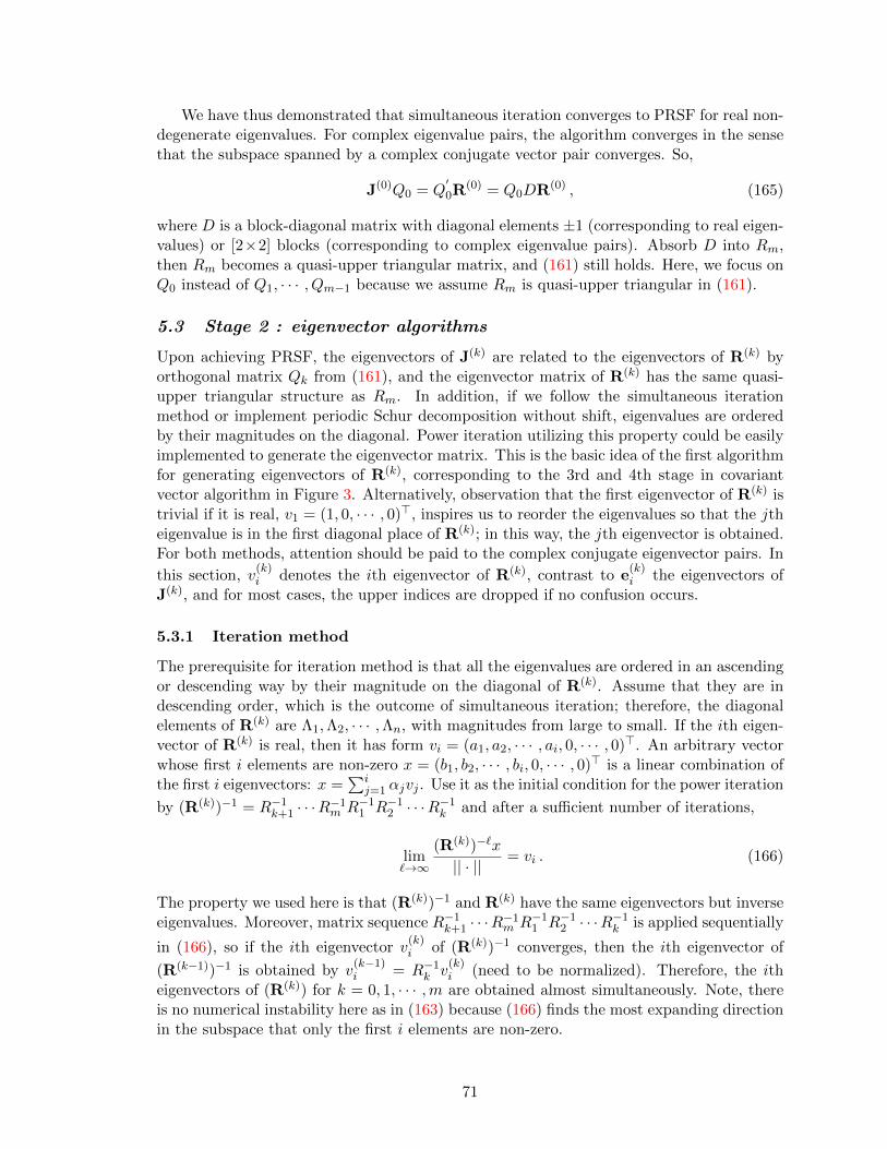
We have thus demonstrated that simultaneous iteration converges to PRSF for real non-degenerate eigenvalues. For complex eigenvalue pairs, the algorithm converges in the sensethat the subspace spanned by a complex conjugate vector pair converges. So,

J(0)Q0 = Q′0R

(0) = Q0DR(0) , (165)

where D is a block-diagonal matrix with diagonal elements ±1 (corresponding to real eigen-values) or [2×2] blocks (corresponding to complex eigenvalue pairs). Absorb D into Rm,then Rm becomes a quasi-upper triangular matrix, and (161) still holds. Here, we focus onQ0 instead of Q1, · · · , Qm−1 because we assume Rm is quasi-upper triangular in (161).

5.3 Stage 2 : eigenvector algorithms

Upon achieving PRSF, the eigenvectors of J(k) are related to the eigenvectors of R(k) byorthogonal matrix Qk from (161), and the eigenvector matrix of R(k) has the same quasi-upper triangular structure as Rm. In addition, if we follow the simultaneous iterationmethod or implement periodic Schur decomposition without shift, eigenvalues are orderedby their magnitudes on the diagonal. Power iteration utilizing this property could be easilyimplemented to generate the eigenvector matrix. This is the basic idea of the first algorithmfor generating eigenvectors of R(k), corresponding to the 3rd and 4th stage in covariantvector algorithm in Figure 3. Alternatively, observation that the first eigenvector of R(k) istrivial if it is real, v1 = (1, 0, · · · , 0)>, inspires us to reorder the eigenvalues so that the jtheigenvalue is in the first diagonal place of R(k); in this way, the jth eigenvector is obtained.For both methods, attention should be paid to the complex conjugate eigenvector pairs. In

this section, v(k)i denotes the ith eigenvector of R(k), contrast to e

(k)i the eigenvectors of

J(k), and for most cases, the upper indices are dropped if no confusion occurs.

5.3.1 Iteration method

The prerequisite for iteration method is that all the eigenvalues are ordered in an ascendingor descending way by their magnitude on the diagonal of R(k). Assume that they are indescending order, which is the outcome of simultaneous iteration; therefore, the diagonalelements of R(k) are Λ1,Λ2, · · · ,Λn, with magnitudes from large to small. If the ith eigen-vector of R(k) is real, then it has form vi = (a1, a2, · · · , ai, 0, · · · , 0)>. An arbitrary vectorwhose first i elements are non-zero x = (b1, b2, · · · , bi, 0, · · · , 0)> is a linear combination ofthe first i eigenvectors: x =

∑ij=1 αjvj . Use it as the initial condition for the power iteration

by (R(k))−1 = R−1k+1 · · ·R−1

m R−11 R−1

2 · · ·R−1k and after a sufficient number of iterations,

lim`→∞

(R(k))−`x

|| · || = vi . (166)

The property we used here is that (R(k))−1 and R(k) have the same eigenvectors but inverseeigenvalues. Moreover, matrix sequence R−1

k+1 · · ·R−1m R−1

1 R−12 · · ·R−1

k is applied sequentially

in (166), so if the ith eigenvector v(k)i of (R(k))−1 converges, then the ith eigenvector of

(R(k−1))−1 is obtained by v(k−1)i = R−1

k v(k)i (need to be normalized). Therefore, the ith

eigenvectors of (R(k)) for k = 0, 1, · · · ,m are obtained almost simultaneously. Note, thereis no numerical instability here as in (163) because (166) finds the most expanding directionin the subspace that only the first i elements are non-zero.

71

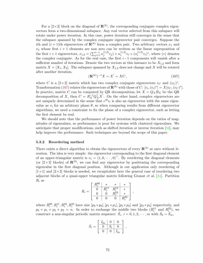
For a [2×2] block on the diagonal of R(k), the corresponding conjugate complex eigen-vectors form a two-dimensional subspace. Any real vector selected from this subspace willrotate under power iteration. In this case, power iteration still converges in the sense thatthe subspace spanned by the complex conjugate eigenvector pair converges. Suppose theith and (i + 1)th eigenvectors of R(k) form a complex pair. Two arbitrary vectors x1 andx2 whose first i + 1 elements are non zero can be written as the linear superposition of

the first i+ 1 eigenvectors, x1,2 = (∑i−1

j=1 α(1,2)j vj) + α

(1,2)i vi + (α

(1,2)i vi)

∗, where (∗) denotesthe complex conjugate. As for the real case, the first i−1 components will vanish after asufficient number of iterations. Denote the two vectors at this instance to be X1,2 and formmatrix X = [X1, X2]. The subspace spanned by X1,2 does not change and X will be rotatedafter another iteration,

(R(k))−1X = X′

= XC , (167)

where C is a [2×2] matrix which has two complex conjugate eigenvectors vC and (vC)∗.Transformation (167) relates the eigenvectors of R(k) with those of C: [vi, (vi)

∗] = X[vC , (vC)∗].In practice, matrix C can be computed by QR decomposition; let X = QXRX be the QRdecomposition of X, then C = R−1

X Q>XX′. On the other hand, complex eigenvectors are

not uniquely determined in the sense that eiθvi is also an eigenvector with the same eigen-value as vi for an arbitrary phase θ, so when comparing results from different eigenvectoralgorithms, we need a constraint to fix the phase of a complex eigenvector, such as lettingthe first element be real.

We should note that the performance of power iteration depends on the ratios of mag-nitudes of eigenvalues, so performance is poor for systems with clustered eigenvalues. Weanticipate that proper modifications, such as shifted iteration or inverse iteration [84], mayhelp improve the performance. Such techniques are beyond the scope of this paper.

5.3.2 Reordering method

There exists a direct algorithm to obtain the eigenvectors of every R(k) at once without it-eration. The idea is very simple: the eigenvector corresponding to the first diagonal elementof an upper-triangular matrix is v1 = (1, 0, · · · , 0)>. By reordering the diagonal elements(or [2×2] blocks) of R(0), we can find any eigenvector by positioning the correspondingeigenvalue in the first diagonal position. Although in our application only reordering of[1×1] and [2×2] blocks is needed, we recapitulate here the general case of reordering twoadjacent blocks of a quasi-upper triangular matrix following Granat et al. [44]. PartitionRi as

Ri =

R00i ∗ ∗ ∗0 R11

i R12i ∗

0 0 R22i ∗

0 0 0 R33i

,where R00

i , R11i , R

22i , R

33i have size [p0×p0], [p1×p1], [p2×p2] and [p3×p3] respectively, and

p0 + p1 + p2 + p3 = n. In order to exchange the middle two blocks (R11i and R22

i ), weconstruct a non-singular periodic matrix sequence: Si, i = 0, 1, 2, · · · ,m with S0 = Sm,

Si =

Ip0 0 0

0 Si 0

0 0 Ip3

,

72

where Si is a [(p1 + p2)×(p1 + p2)] matrix, such that Si transforms Ri as follows:

S−1i RiSi−1 = Ri =

R00i ∗ ∗ ∗0 R22

i 0 ∗0 0 R11

i ∗0 0 0 R33

i

, (168)

which is

S−1i

[R11i R12

i

0 R22i

]Si−1 =

[R22i 00 R11

i

].

The problem is to find the appropriate matrices Si which satisfy the above condition.Assume Si has form

Si =

[Xi Ip1Ip2 0

],

where matrix Xi has dimension [p1×p2]. We obtain periodic Sylvester equation [44]

R11i Xi−1 −XiR

22i = −R12

i , i = 0, 1, 2, · · · ,m . (169)

The algorithm to find eigenvectors is based on (169). If the ith eigenvalue of R(k) isreal, we only need to exchange the leading [(i−1)×(i−1)] block of Rk , k = 1, 2, · · · ,m withits ith diagonal element. If the ith and (i+1)th eigenvalues form a complex conjugate pair,then the leading [(i− 1)×(i− 1)] block and the following [2×2] block should be exchanged.Therefore Xi in (169) has dimension [p1×1] or [p1×2]. In both cases, p0 = 0.

Real eigenvectors In this case, matrix Xi is just a column vector, so (169) is equivalentto

R111 −R22

1 Ip1

R112 −R22

2 Ip1

R113 −R22

3 Ip1

. . . · · ·

−R22m Ip1 R11

m

X0

X1

X2

· · ·

Xm−1

=

−R121

−R122

−R123

· · ·

−R12m

, (170)

where R22i is the (p1 + 1)th diagonal element of Ri. The accuracy of eigenvectors is deter-

mined by the accuracy of solving sparse linear equation (170). In our application to periodicorbits in the one-dimensional Kuramoto-Sivashinsky equation, Gaussian elimination withpartial pivoting is enough. For a more technical treatment, such as cyclic reduction orpreconditioned conjugate gradients, to name a few, please see [1, 30, 45].

Now we get all vectors Xi by solving periodic Sylvester equation, but how are theyrelated to the eigenvectors? In analogy to R(0), defining R0 = RmRm−1 · · · R1, we getS−1m R(0)Sm = R0 by (168). Since p0 = 0 and p2 = 1 in (168), the first eigenvector of R0,

the one corresponding to eigenvalue Λp1+1 is e = (1, 0, · · · , 0)>. Apart from normalization,the corresponding eigenvector of R(0) is

v(0)p1+1 = Sme =

[X>0 , 1, 0, 0, · · · , 0

]>.

73

This is the eigenvector of matrix R(0) = RmRm−1 · · ·R1 in (162) for k = 0. For R(1) =R1Rm · · ·R2, the corresponding periodic Sylvester equation will be cyclically rotated onerow up in (170), which means X1 will be shifted to the first place, and thus the corre-

sponding eigenvector of R(1) is v(1)p1+1 = [X>1 , 1, 0, · · · , 0]>. The same argument goes for

all the remaining R(k). In conclusion, solution of (170) contains the eigenvectors for allR(k) , k = 0, 1, · · · ,m − 1. Another benefit of reordering method is that we can selectivelyget the eigenvectors corresponding to some specific eigenvalues. This merit is important inhigh-dimensional nonlinear systems for which only a subset of Floquet vectors suffices tocharacterize the dynamics in tangent space, and thus we avoid wasting time in calculatingthe remaining unimportant subset.

Complex eigenvector pairs As in the real eigenvalue case, we have p0 = 0, but nowp2 = 2, so matrix Xi has dimension [p1×2]. Using the same notation as ref. [44], let v(Xi)denote the vector representation of Xi with the columns of Xi stacked on top of each other,and let A⊗B denote the Kronecker product of two matrices, with the (i, j)-block elementbe aijB.

Now, the periodic Sylvester equation (169) is equivalent to

I2 ⊗R111 −(R22

1 )> ⊗ Ip1

I2 ⊗R112 −(R22

2 )> ⊗ Ip1

I2 ⊗R113 −(R22

3 )> ⊗ Ip1. . . · · ·

−(R22m )> ⊗ Ip1 I2 ⊗R11

m

v(X0)

v(X1)

v(X2)

· · ·

v(Xm−1)

=

−v(R121 )

−v(R122 )

−v(R123 )

· · ·

−v(R12m )

.

(171)After switching R11

i and R22i , we can get the first two eigenvectors of R0 by multiplying the

first [2×2] diagonal blocks of Ri: R22 = R22

mR22m−1 · · ·R22

1 . Let the eigenvectors of R22 be v

and v∗ of size [2×1], then the corresponding eigenvectors of R0 are e1 = (v>, 0, 0, · · · , 0)>

and e2 = (e1)∗ (the additional zeros make the length of the eigenvectors be n). Therefore,the corresponding eigenvectors of R(0) are

[v

(0)p1+1, v

(0)p1+2

]= Sm[e1, e2] =

X0

I2

0 00 0

...0 0

[v, v∗] .

For other R(k), the same argument in the real case applies here too, so we obtain all thecomplex eigenvector pairs for R(k) , k = 1, 2, · · · ,m.

5.4 Computational complexity and convergence analysis

In this section, we make no attempt at conducting a strict error analysis of the algorithmspresented. However, for practical applications, it is important to understand their compu-tational costs. Periodic eigendecomposition is conducted in two stages: (1) PRSF, and (2)

74

determination of all eigenvectors. In each stage, there are two candidate algorithms, so theefficiency of periodic eigendecomposition depends on the choice of the specific algorithmchosen in each stage.

Periodic Schur decomposition algorithm and simultaneous iteration are both effectiveto achieve PRSF. We estimate the complexity of periodic Schur decomposition algorithmin analogy with the single matrix case. For a single [n×n] matrix, O(n3) flops (floating-point operations) are required [84] to reduce it to upper Hessenberg form. Accordingly,the first stage in Figure 4 takes O(mn3) flops. Then the implicit QR iteration processfor a single matrix takes O(n2) flops for a single iteration, so each iteration of the secondstage in Figure 4 takes O(mn2) flops. Usually, the number of iterations exceeds by far thedimension of the matrix. Therefore, the average complexity of one iteration in periodic Schurdecomposition algorithm is O(mn2). For a detailed discussion see [8, 84]. On the other hand,simultaneous iteration (164) requires m QR decomposition O(mn3) and m matrix-matrixmultiplication O(mn3) in each iteration, giving a total computational cost of O(mn3).Moreover, the convergence of both algorithms depends linearly on the ratio of adjacenteigenvalues of R(0): |Λi|/|Λi+1| without shift [37]. Therefore, the ratio of costs betweenperiodic Schur decomposition algorithm and simultaneous iteration is approximately ofthe order O(mn2)/O(mn3) = O(1/n), implying that the periodic Schur decompositionalgorithm is much cheaper than the simultaneous iteration if the dimension of matricesinvolved is large.

The second stage of periodic eigendecomposition is to find all the eigenvectors of J(k) viaquasi-upper triangular matrices R(k). The first candidate is power iteration. The computa-tional cost of one iteration (166) for the ith eigenvector is O(mi2). The second candidate,reordering method, relies on an effective method to solve periodic Sylvester equation (169).For example, Gaussian elimination with partial pivoting is suitable for well-conditioned ma-trix (170) and (171) with a computational cost of O(mi2) for the ith eigenvector. Here, wehave taken account of the sparse structure of (170) and (171). For a detailed discussion,see ref. [44]. So, the total complexity of reordering method is approximately the same asthat of one iteration in power iteration.

In summary, if we only consider the computational complexity, the combination ofperiodic Schur decomposition algorithm and reordering method is preferable for periodiceigendecomposition.

5.5 Application to Kuramoto-Sivashinsky equation

Our ultimate goal of implementing periodic eigendecomposition is to analyze the stability ofperiodic orbits and the associated stable/unstable manifolds in dynamical systems, for thehope of getting a better understanding of pattern formation and turbulence. As an example,we focus on the one-dimensional Kuramoto-Sivashinsky equation(134) and its Fourier spaceform (135). We follow Sect. 3.1 to integrate this system. For the calculation of Floquetspectrum and vectors, we use the combination of periodic Schur decomposition algorithmand reordering algorithm. In addition, Gaussian elimination with partial pivoting is stablefor solving (170) and (171) if the time step in Kuramoto-Sivashinsky integrator is not toolarge.

Here we show how well periodic eigendecomposition works by applying it to one repre-sentative preperiodic orbit ppo10.25 (the 1st subplot in Figure 15) and two relative periodicorbits rpo16.31 (the 4th subplot in Figure 15) and rpo57.60 which is documented in ref. [21].

75

5.5.1 Accuracy

Table 7 shows that the 2nd and 3rd, respectively 3rd and 4th exponents of rpo16.31, re-spectively ppo10.25, are marginal. Even though the inaccuracy of the closure of the orbitcontributes to the error, we note that the absolute error takes values as low as 10−12. Table 7and Figure 17 show that periodic Schur decomposition is capable of resolving Floquet mul-tipliers differing by thousands of orders of magnitude: when using N = 64 Fourier modes,the smallest Floquet multiplier magnitude for ppo10.25 is |Λ62| ' e−6080.4×10.25 ' 10−27067.This cannot be achieved if we try to compute a single Jacobian matrix for the whole orbit.

Figure 28: Marginal vectors and the associated errors. (a) ppo10.25 in one period projectedinto [b1, c1, b2] subspace (blue curve), and its counterpart (green line) generated by a smallgroup transformation g(φ) , here arbitrarily set to φ = 0.1. Magenta and black arrowsrepresent the first and the second marginal Floquet vectors e3(x) and e4(x) along theprime orbit. (b) The solid red curve is the Euclidean difference between e3(x) and thevelocity field v(x) along the orbit, and the blue dashed curve is the difference between e4(x)and the group tangent t(x) = Tx.

The two marginal directions have a simple geometrical interpretation and provide ametric for us to measure the convergence of periodic eigendecomposition. Figure 28 (a)depicts the two marginal vectors of ppo10.25 projected into the subspace spanned by [b1, c1, b2](the real, imaginary parts of the first mode and the real part of the second Fourier mode).The first marginal direction (the 3rd Floquet vector in Table 7) is aligned with the velocityfield along the orbit, and the second marginal direction (the 4th Floquet vector) is alignedwith the group tangent. The numerical difference between the unit vectors along these twomarginal directions and the corresponding physical directions is shown in Figure 28 (b). Thedifference is under 10−9 and 10−11 for these two directions, which demonstrates the accuracyof the algorithm. As shown in Table 7, for a preperiodic orbit, such as ppo10.25, the velocityfield and the group tangent have eigenvalue +1 and −1 respectively, and are thus distinct.However, the two marginal directions are degenerate for a relative periodic orbit, such asrpo16.31. So these two directions are not fixed, but the two-dimensional plane spanned bythem is uniquely determined. Figure 29 shows that the velocity field and group tangent

76

along orbit rpo16.31 indeed lie in the subspace spanned by these two marginal directions.

Figure 29: Projection of relative periodic orbit rpo16.31 into the Fourier modes subspace[b2, c2, b3] (red curve). The dotted curve (lime) is the group orbit connecting the initial andfinal points. Blue and magenta arrows represent the velocity field and group tangent alongthe orbit, respectively. Two-dimensional planes (cyan) are spanned by the two marginalFloquet vectors at each point (yellow) along the orbit.

5.5.2 The choice of the number of orbit segments

We have noted above that the semi-group property of Jacobian matrix (31) enables us tofactorize J(k) into a product of short-time matrices with matrix elements of comparableorder of magnitude. In practice, caution should be exercised when trying to determine theoptimal number of time increments that the orbit should be divided into. If the number oftime incrementsm is too large, then, according to the estimates of Sect. 5.4, the computationmay be too costly. If m is too small, then the elements of the Jacobian matrix correspondingto the corresponding time increment may range over too many orders of magnitude, causingperiodic eigendecomposition to fail to resolve the most contracting Floquet vector along theorbit. One might also vary the time step according to the velocity at a given point onthe orbit. Here we determined satisfactory m’s by numerical experimentation shown inFigure 30. Since larger time step means fewer time increments of the orbit, a very smalltime step (h0 ≈ 0.001) is chosen as the base case, and it is increased to test whether thecorresponding Floquet exponents change substantially or not. As shown in Figure 30 (a),up to 6h0 the whole Floquet spectrum varies within 10−12 for both ppo10.25 and rp57.60.These two orbits represent two different types of invariant solutions which have short andlong periods respectively, so we presume that time step 6h0 is good enough for other short orlong orbits too. On the other hand, if only the first few Floquet exponents are desired, thetime step can be increased further to fulfill the job. As shown in Figure 30 (b), if we are onlyinterested in the first 35 Floquet exponents, then time step 30h0 is small enough. In high-dimensional nonlinear systems, often we are not interested in very contraction directions

77

Figure 30: Relative error of the real part of Floquet exponents associated with differenttime steps with which the Floquet matrix is integrated. Two orbits ppo10.25 and rpo57.60

are used as an example with the base case h0 ≈ 0.001. (a) The maximal relative differenceof the whole set of Floquet exponents with increasing time step (decreasing the number ofingredient segments of the orbit). (b) Only consider the first 35 Floquet exponents.

because dynamics in these directions are transient and shed little insight into the systemproperties. Therefore, large time step could be used to save time.

5.6 Conclusion and future work

In this chapter we have used the one-dimensional Kuramoto-Sivashinsky system to illustratethe effectiveness of periodic eigendecomposition applied to stability analysis in dissipativenonlinear systems. In future, we hope to apply the method to the study of orbits of muchlonger periods, as well as to the study of high-dimensional numerically exact time-recurrentunstable solutions of the full Navier-Stokes equations. We anticipate the need for optimizingand parallelizing such algorithms. Also, if periodic eigendecomposition is to be applied toHamiltonian systems, additional adjustments will be required to guarantee the preservationof symmetries of Floquet spectrum imposed by the symplectic structure of Hamiltonianflows.

78

CHAPTER VI

CONCLUSION AND FUTURE WORK

In this thesis, we have investigated the dimension of the inertial manifold in the one-dimensional Kuramoto-Sivashinsky equation and determined that the dimension is 8 fordomain size 22. In order to reach this conclusion, we had to develop a number of the-oretical and numerical tools. Here, we summarize the contributions of this thesis in twocategories, theoretical and numerical contributions, and discuss open future directions.

6.1 Theoretical contributions

In Sect. 2.2.2, we define the projection operator from full state space to the slice. Also, inSect. 2.2.3, we give the precise relation between the in-slice Jacobian and the Jacobian inthe full state space. Therefore, in-slice stability eigenvectors can be obtained easily fromthose in the full state space.

In Sect. 3.5.1, we reduce the O(2) symmetry by using the fundamental domain andargue that defining the 1st mode slice to have vanishing real part of the first Fourier modewill keep the reflection rule unchanged in the slice. Such a simplification can be adopted inother systems with O(2) symmetry too, such as complex Ginzburg-Landau equation.

In Sect. 4.2, we use three different numerical approaches, i.e., local Floquet expo-nents, principal angles obtained by Floquet vectors, and expansion errors of differencevectors in shadowing incidences, to estimate the dimension of the inertial manifold in one-dimensional Kuramoto-Sivashinsky equation. The results are consistent among all thesethree approaches and with the previous research on covariant Lyapunov vectors conductedon ergodic trajectories.

6.2 Numerical contributions

In Chapter 5, we provide a detailed description of the periodic eigendecomposition needed tocalculate the stability of periodic orbits of a chaotic system. Its effectiveness and accuracyare tested in the one-dimensional Kuramoto-Sivashinsky equation in Sect. 5.5. The C++

implementation can be found at my GitHub repository github.com/dingxiong/research.This repository also contains the C++ implementation of some other algorithms that

are frequently used in the study of chaotic systems, such as GMRES [74] to solve linearequation Ax = b by Krylov subspace iteration, Levenberg-Marquardt algorithm [59, 62],inexact Newton backtracking method [77], Newton-GMRES-Hookstep algorithm [15] to find(relative) periodic orbits, and the integrator for the one-dimensional Kuramoto-Sivashinskyequation.

6.3 Future work

In this section, I list two potential directions for the future research in this field.

79

6.3.1 Spatiotemporal averages in Kuramoto-Sivashinsky equation

We have gained valuable intuition about the geometrical structure of the global attractor bythe experience of working with these shadowing cases in Sect. 3.5. We observe that the globalattractor has a very thin structure. Orbits can shadow the unstable manifold of E2 anddifferent orbits can shadow each other. Experience with such shadowing incidences helpsus choose appropriate Poincare sections to capture the transition rules between differentsubregions. One is in a position to investigate the symbolic dynamics of the system. Namely,one can try to partition the fundamental domain into several subregions and figure out thetransition rule between different subregions. This transition rule, also called the symbolicdynamics, helps us classify the over 60 000 pre/relative periodic orbits by their topologicallengths. Then the spectral determinant (73) could be accurately approximated by theshortest pre/relative periodic orbits. If this is implemented, spatiotemporal averages couldbe obtained efficiently, without longtime simulations.

6.3.2 The dimensions of inertial manifolds of other systems

We believe that the numerical techniques developed in Chapter 4 can be used to determinethe dimensions of inertial manifolds for other nonlinear dissipative dynamical systems. Theprevious studies [79, 89, 90], based on covariant vectors, have estimated the dimension ofthe inertial manifold of the one-dimensional complex Ginzburg-Landau equation,

At = A+ (1 + iα)Axx − (1 + iβ)|A|2A ,

where A(x, t) is a complex field, and α and β are real parameters. As shown in Figure 31,one-dimensional complex Ginzburg-Landau equation exhibits spatiotemporal chaos similarto the Kuramoto-Sivashinsky Figure 11. We believe (but have not carried out the requisitecomputations) that the analysis based on relative periodic orbits will also in this casedetermine the dimension of inertial manifold. Similar to the one-dimensional Kuramoto-Sivashinsky equation, this equation has a spatial reflection symmetry A(x, t) → A(−x, t)and SO(2)×SO(2) spatial and phase translational symmetries A(x, t)→ eiφA(x+`, t). Thusthe symmetry-reduction techniques discussed in Sect. 2.2 can also be applied here, and onecan restrict the analysis to a fundamental domain in a slice, as we did in Sect. 3.5.1. In twopubications not reported in detail in this thesis [25, 26], we have constructed a “minimal”spatial domain and have determined a variety of equilibria, relative equilibria, and relativeperiodic orbits for this system. This sets the stage for application of methods discussed inSect. 4.2, i.e., evaluation of local Floquet exponents, principal angles among sets of Floquetvectors, and expansion errors of difference vectors during close shadowing episodes, in orderto estimate dimensions of the inertial manifold in system of complex Ginzburg-Landau type.

80

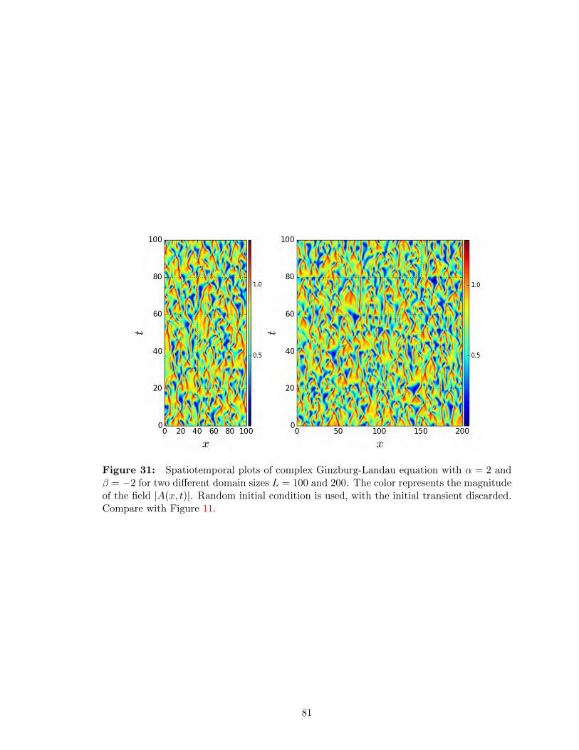
Figure 31: Spatiotemporal plots of complex Ginzburg-Landau equation with α = 2 andβ = −2 for two different domain sizes L = 100 and 200. The color represents the magnitudeof the field |A(x, t)|. Random initial condition is used, with the initial transient discarded.Compare with Figure 11.

81

APPENDIX A

FLOQUET THEOREM AND PERIODIC ORBITS

A linear ordinary differential equation with periodic coefficients is an old topic. Solutionsof such type of equations can be decomposed into the product of a time-exponential partand a bounded periodic part. The rigorous statement is given by

Theorem A.1 [32] If Φ(t) is a fundamental matrix solution of linear system x = A(t)xwith periodic coefficients A(t+ T ) = A(t), T being the period, then Φ(t) can be decomposedas

Φ(t) = P (t)etB with P (t) = P (t+ T ) .

Here P (t) is called monodromy matrix, and B is a constant matrix. Eigenvalues of B arecalled Floquet exponents. The eigenvectors are called Floquet vectors.

The proof of this theorem is very simple. First, it is easy to see that if Φ(t) is solutionmatrix, so is Φ(t+ T ). Their relation is given by Φ(t+ T ) = Φ(t)C(t, T ), where C(t, T ) =Φ−1(t)Φ(t+T ). Second, C(t, T ) is independent of time which can be shown by taking timederivative at both sides of Φ(t)C(t, T ) = Φ(t+ T ),

Φ(t)C(t, T ) + Φ(t)C(t, T ) = Φ(t+ T )

=⇒ A(t)Φ(t)C(t, T ) + Φ(t)C(t, T ) = A(t+ T )Φ(t+ T )

=⇒ C(t, T ) = 0 .

So matrix C(T ) is only parametrized by the period. Furthermore,

C(nT ) =n−1∏k=0

(Φ−1(t+ kT ) Φ(t+ (k + 1)T )

)= C(T )n ;

thus C(T ) has form eTB, where B is a constant matrix. So Φ(t + T ) = Φ(t)eTB. Last, Ifwe define a new matrix P (t) = Φ(t)e−tB, then

P (t+ T ) = Φ(t+ T )e−TB−tB = Φ(t)e−tB = P (t) .

In this way, we decompose the fundamental matrix solution into a periodic part P (t) anda time exponential part etB, even though we do not know the explicit form of P (t).

Floquet theorem in condensed matter physics is under another name: Bloch theorem,

which states that wave function in a periodic potential can be written as ψ(~r) = ei~k·~ru(~r).

Here u(~r) is a periodic function with the same potential period. Eigenstates are classifiedinto different bands by different profiles of u(~r).

For our interest, dynamics in the tangent space in a nonlinear dynamical system isgoverned by J = AJ . Especially, for periodic orbits, A is periodic, and if we start withJ(t0) = I, then Jacobian corresponding to one period Jp is just the exponential part eTB intheorem A.1. This is the theoretical basis of periodic eigendecomposition algorithm, whichtries to calculate the eigenvalues and eigenvectors of Jp. On the other hand, the periodicpart P (t) in theorem A.1 evolves Floquet vectors along the periodic orbit, and returns tothe initial value after one period. This information is revealed in the reordering stage ofperiodic eigendecomposition algorithm.

82

APPENDIX B

PROOF OF PROPOSITION 4.2

The proof of proposition 4.2 provided by Collet et al. [17] concerns the calculation in theFourier space. Let

v(x, t) = i

∞∑n=−∞

vn(t)einqx , Φx(x) = −∞∑

n=−∞ψne

inqx

with q = 2π/L. Here, we modify the form of Fourier transform by taking into considerationthe fact that both v(x, t) and Φ(x) are antisymmetric. Therefore, vn and ψn are all realnumbers and we have relations

vn = −v−n , ψn = ψ−n . (172)

We also impose ψ0 = 0. Note that we define the Fourier mode for Φx(x) not Φ(x). Withthis setup, now we try to prove (148). We first calculate

∫v2Φx(x) and

∫v(∂2

x + ∂4x)v.∫

v2Φx(x) =∑k,l,m

∫vkvlψme

i(k+l+m)qx

= L∑

k+l+m=0

vkvlψm = L∑k,l

vkvlψ−k−l = L∑k,l

vkvlψ|k+l| .

∫v(∂2

x + ∂4x)v =

∑k,l

∫vk(−n2q2 + n4q4)vle

i(k+l)qx

= L∑k

(−n2q2 + n4q4)v2k .

In the above derivation, we have used relation (172) and ψ0 = 0. Then

(v, v)γΦ =

∫v(∂2

x + ∂4x + γΦx)v

= L∑k

(−n2q2 + n4q4)v2k + γL

∑k,l

vkvlψ|k+l|

= 2L∑k>0

(−n2q2 + n4q4)v2k + γL

∑k,l>0

vkvl(ψ|k+l| + ψ|−k−l| − ψ|k−l| − ψ|−k+l|)

= 2L

∑k>0

(−n2q2 + n4q4)v2k + γ

∑k,l>0

vkvl(ψ|k+l| − ψ|k−l|)

= 2L

∑k>0

(−n2q2 + n4q4 + γψ2k)v2k + γ

∑k,l>0k 6=m

vkvl(ψ|k+l| − ψ|k−l|)

= 2L

(∑k>0

(−n2q2 + n4q4 + γψ2k)v2k + 2γ

∑k>l>0

vkvl(ψk+l − ψ|k−l|))

(173)

83

and

1

4

∫(v2xx + v2) = −1

4

∑k,l

∫vk(n

4q4 + 1)vlei(k+l)qx

=L

4

∑k

(n4q4 + 1)v2k

=L

2

∑k>0

(n4q4 + 1)v2k . (174)

In order to show (v, v)γΦ ≥ 14

∫(v2xx + v2), we choose as ψn as follows

ψn =

0, for n odd{

4, when 1 ≤ |n| ≤ 2M

4f(|n|/2M − 1), when 2M ≤ |n|, for n even

. (175)

Here f(n) is a non-increasing function whose first-order derivative is continuous. It satisfiesf(0) = 1, f ′(0) = 0 and

f ≥ 0 , sup |f ′| < 1 ,

∫ ∞0

dk(1 + k)2|f(k)|2 <∞ . (176)

Integer M satisfies

M ≥ 2

q(177)

and its exact value will be determined later. Therefore

−n2q2 + n4q4 + γψ2k =1

2(n2q2 − 1)2 +

1

2(n4q4 + 1) + γψ2k − 1

≥ 1

2(n4q4 + 1) .

Here, we have used the fact that ψ2k > 0 when nq > 2 and ψ2k > 4 when nq ≤ 2 togetherwith γ ∈ [1/4, 1]. With this inequality, we try to give lower bound of (173). Before that,for notation convenience, we define

τn =

√q4n4 + 1

2, ωn = τnvn . (178)

Then from (173) we have

(v, v)γΦ ≥ 2L

(∑k>0

ω2k + 2γ

∑k>l>0

ωkψk+l − ψ|k−l|

τkτlωl

).

and (174) becomes1

4

∫(v2xx + v2) = L

∑k>0

ω2k .

In order to make (v, v)γΦ ≥ 14

∫(v2xx + v2), we need to prove∑

k>0

ω2k + 4γ

∑k>l>0

ωkψk+l − ψ|k−l|

τkτlωl > 0

84

for γ ∈ [1/4, 1]. One sufficient but not necessary condition is∑k>l>0

∣∣∣∣ψk+l − ψ|k−l|τkτl

∣∣∣∣2 < 1

16.

Now, we show that the above relation is valid given the choice of ψk in (175).

∑k>l>0

∣∣∣∣ψk+l − ψ|k−l|τkτl

∣∣∣∣2=

∞∑m=1

τ−2m

∞∑k=m+1

(ψk+m − ψk−m)2τ−2k

≤ 16

M2

M∑m=1

m2τ−2m

∞∑k=2M−m+1

τ−2k +

16

M2

∞∑m=M+1

m2τ−2m

∞∑k=m+1

τ−2k

≤ 16

M2

M∑m=1

m2τ−2m

∫ ∞2M−m

τ−2k dk +

16

M2

∞∑m=M+1

m2τ−2m

∫ ∞m

τ−2k dk

=32

M2

M∑m=1

m2τ−2m

∫ ∞2M−m

1

q4k4 + 1dk +

32

M2

∞∑m=M+1

m2τ−2m

∫ ∞m

1

q4k4 + 1dk

≤ 32

M2

M∑m=1

m2τ−2m

∫ ∞2M−m

1

q4k4dk +

32

M2

∞∑m=M+1

m2τ−2m

∫ ∞m

1

q4k4dk

=32

3M2q4

M∑m=1

m2τ−2m

1

(2M −m)3+

32

3M2q4

∞∑m=M+1

m2τ−2m

1

m3

≤ 32

3M5q4

M∑m=1

m2τ−2m +

32

3M2q4

∞∑m=M+1

m−1τ−2m

≤ 64

3M5q4

∫ ∞0

m2

q4m4 + 1dm+

64

3M2q4

∫ ∞M

1

m(q4m4 + 1)dm

≤ 64

3M5q4

∫ ∞0

m2

(q4m4 + 1)1/2(q4m4)1/2dm+

64

3M2q4

∫ ∞M

1

m(q4m4)dm

≤ 64

3M5q6

∫ ∞0

1

(q4m4 + 1)1/2dm+

16

3M6q8

=64

3M5q6

4Γ(54)2

√πq

+16

3M6q8

<128

3M5q7+

16

3M6q8.

We choose M to be the smallest integer larger than 4q−7/5 = 4(L/2π)7/5, then

128

3M5q7+

16

3M6q8<

128

3 · 45+

16

3 · 46q−2/5<

11

256<

1

16.

In the above derivation, we have used the fact that q = 2π/L < 1. Also, note that the choiceof M here satisfies the requirement (177). Therefore, (148) in proposition 4.2 is validated.Now we turn to the proof of (149).

85

(Φ,Φ)γΦ =

∫ L

0Φ(∂2

x + ∂4x)Φdx

= −∫ L

0Φx(∂x + ∂3

x)Φdx

= −∫ L

0

∑m,n

ψm(1− n2q2)ψnei(m+n)qxdx

= 2L

∞∑n=1

(n2q2 − 1)ψ2n

= 2L

(2M∑n=1

(n2q2 − 1)16 +

∞∑n=2M+1

(n2q2 − 1)16f2(n

2M− 1)

)

≤ 32L

(2M(2M)2q2 +

∫ ∞2M+1

dn(n2q2 − 1)f2(n

2M− 1)

)≤ 32L

(8M3q2 +

∫ ∞0

dn2M((n+ 1)24M2q2 − 1)f2(n)

)≤ 256LM3q2

(1 +

∫ ∞0

dn(n+ 1)2f2(n)

)= 256L

(4(

2π

L)−7/5

)3(2π

L

)2(1 +

∫ ∞0

dn(n+ 1)2f2(n)

)= KL16/5

(1 +

∫ ∞0

dn(n+ 1)2f2(n)

).

From (176), we know that (149) is verified. Thus, we finish the proof of proposition 4.2.

86

References

[1] P. Amodio, J. R. Cash, G. Roussos, R. W. Wright, G. Fairweather, I. Gladwell, G.L. Kraut, and M. Paprzycki, “Almost block diagonal linear systems: sequential andparallel solution techniques, and applications”, Numer. Linear Algebra Appl. 7, 275–317 (2000).

[2] I. S. Aranson and L. Kramer, “The world of complex Ginzburg-Landau equation”,Rev. Mod. Phys. 74, 99–143 (2002).

[3] R. Artuso, E. Aurell, and P. Cvitanovic, “Recycling of strange sets: I. Cycle expan-sions”, Nonlinearity 3, 325–359 (1990).

[4] R. Artuso, E. Aurell, and P. Cvitanovic, “Recycling of strange sets: II. Applications”,Nonlinearity 3, 361–386 (1990).

[5] G. Benettin, L. Galgani, A. Giorgilli, and J. M. Strelcyn, “Lyapunov characteristicexponents for smooth dynamical systems and for Hamiltonian systems; a method forcomputing all of them. Part 1: theory”, Meccanica 15, 9–20 (1980).

[6] A. Bjorck and G. H. Golub, “Numerical methods for computing angles between linearsubspaces”, Math. Comput. 27, 579–594 (1973).

[7] J. Bochi and M. Viana, “How frequently are dynamical systems hyperbolic?”, in Mod-ern dynamical systems and applications, edited by M. Brin, B. Hasselblatt, and Y.Pesin (Cambridge Univ. Press, Cambridge, 2004), pp. 271–297.

[8] A. Bojanczyk, G. H. Golub, and P. V. Dooren, The periodic Schur decomposition.Algorithms and applications, in Proc. SPIE Conference (1992), pp. 31–42.

[9] H. Bosetti and H. A. Posch, “What does dynamical systems theory teach us aboutfluids?”, Commun. Theor. Phys. 62, 451–468 (2014).

[10] J. C. Bronski and T. N. Gambill, “Uncertainty estimates and L2 bounds for theKuramoto-Sivashinsky equation”, Nonlinearity 19, 2023–2039 (2006).

[11] N. B. Budanur, Exact Coherent Structures in Spatiotemporal Chaos: From QualitativeDescription to Quantitative Predictions, PhD thesis (School of Physics, Georgia Inst.of Technology, Atlanta, 2015).

[12] N. B. Budanur and P. Cvitanovic, “Unstable manifolds of relative periodic orbitsin the symmetry-reduced state space of the Kuramoto-Sivashinsky system”, J. Stat.Phys., 1–20 (2015).

[13] N. B. Budanur, D. Borrero-Echeverry, and P. Cvitanovic, “Periodic orbit analysis ofa system with continuous symmetry - A tutorial”, Chaos 25, 073112 (2015).

[14] N. B. Budanur, P. Cvitanovic, R. L. Davidchack, and E. Siminos, “Reduction of theSO(2) symmetry for spatially extended dynamical systems”, Phys. Rev. Lett. 114,084102 (2015).

[15] G. J. Chandler and R. R. Kerswell, “Invariant recurrent solutions embedded in aturbulent two-dimensional Kolmogorov flow”, J. Fluid Mech. 722, 554–595 (2013).

[16] F. Christiansen, P. Cvitanovic, and V. Putkaradze, “Spatiotemporal chaos in termsof unstable recurrent patterns”, Nonlinearity 10, 55–70 (1997).

87

[17] P. Collet, J. P. Eckmann, H. Epstein, and J. Stubbe, “A global attracting set for theKuramoto-Sivashinsky equation”, Commun. Math. Phys. 152, 203–214 (1993).

[18] P. Constantin, C. Foias, B. Nicolaenko, and R. Temam, Integral manifolds and inertialmanifolds for dissipative partial differential equations (Springer, New York, 1989).

[19] S. M. Cox and P. C. Matthews, “Exponential time differencing for stiff systems”, J.Comput. Phys. 176, 430–455 (2002).

[20] M. C. Cross and P. C. Hohenberg, “Pattern formation outside of equilibrium”, Rev.Mod. Phys. 65, 851–1112 (1993).

[21] P. Cvitanovic, R. L. Davidchack, and E. Siminos, “On the state space geometry ofthe Kuramoto-Sivashinsky flow in a periodic domain”, SIAM J. Appl. Dyn. Syst. 9,1–33 (2010).

[22] P. Cvitanovic, R. Artuso, R. Mainieri, G. Tanner, and G. Vattay, Chaos: Classicaland Quantum (Niels Bohr Inst., Copenhagen, 2017).

[23] R. L. Devaney, Chaos in the Classroom, Boston Univ. 1995.

[24] X. Ding and P. Cvitanovic, “Periodic eigendecomposition and its application in Kuramoto-Sivashinsky system”, SIAM J. Appl. Dyn. Syst. 15, 1434–1454 (2016).

[25] X. Ding and P. Cvitanovic, Exploding relative periodic orbits in cubic-quintic complexGinzburg–Landau equation, In preparation, 2017.

[26] X. Ding and S. H. Kang, Adaptive time-stepping exponential integrators for cubic-quintic complex Ginzburg–Landau equations, 2017.

[27] X. Ding, H. Chate, P. Cvitanovic, E. Siminos, and K. A. Takeuchi, “Estimating thedimension of the inertial manifold from unstable periodic orbits”, Phys. Rev. Lett.117, 024101 (2016).

[28] J.-P. Eckmann and D. Ruelle, “Ergodic theory of chaos and strange attractors”, Rev.Mod. Phys. 57, 617–656 (1985).

[29] S. V. Ershov and A. B. Potapov, “On the concept of stationary Lyapunov basis”,Physica D 118, 167–198 (1998).

[30] G. Fairweather and I. Gladwell, “Algorithms for almost block diagonal linear systems”,SIAM Rev. 46, 49–58 (2004).

[31] J. D. Farmer, E. Ott, and J. A. Yorke, “The dimension of chaotic attractors”, in Thetheory of chaotic attractors, edited by B. R. Hunt, T.-Y. Li, J. A. Kennedy, and H. E.Nusse (Springer, New York, 1983), pp. 142–169.

[32] G. Floquet, “Sur les equations differentielles lineaires a coefficients periodiques”, Ann.Sci. Ec. Norm. Ser 12, 47–88 (1883).

[33] C. Foias, B. Nicolaenko, G. R. Sell, and R. Temam, “Inertial manifold for the Kuramoto-Sivashinsky equation”, C. R. Acad. Sci. Paris, Ser. I 301, 285–288 (1985).

[34] C. Foias, G. R. Sell, and R. Temam, “Inertial manifolds for nonlinear evolutionaryequations”, J. Diff. Equ. 73, 309–353 (1988).

[35] C. Foias, B. Nicolaenko, G. R. Sell, and R. Temam, “Inertial manifolds for theKuramoto-Sivashinsky equation and an estimate of their lowest dimension”, J. Math.Pure Appl. 67, 197–226 (1988).

88

[36] C. Foias, M. S. Jolly, I. G. Kevrekidis, G. R. Sell, and E. S. Titi, “On the computationof inertial manifolds”, Phys. Lett. A 131, 433–436 (1988).

[37] J. G. F. Francis, “The QR transformation: A unitary analogue to the LR transforma-tion. I”, Comput. J. 4, 265–271 (1961).

[38] P. Frederickson, J. L. Kaplan, E. D. Yorke, and J. A. Yorke, “The Liapunov dimensionof strange attractors”, J. Diff. Eqn. 49, 185–207 (1983).

[39] L. Giacomelli and F. Otto, “New bounds for the Kuramoto-Sivashinsky equation”,Commun. Pure Appl. Math. 58, 297–318 (2005).

[40] J. F. Gibson, J. Halcrow, and P. Cvitanovic, “Visualizing the geometry of state-spacein plane Couette flow”, J. Fluid Mech. 611, 107–130 (2008).

[41] F. Ginelli, P. Poggi, A. Turchi, H. Chate, R. Livi, and A. Politi, “Characterizingdynamics with covariant Lyapunov vectors”, Phys. Rev. Lett. 99, 130601 (2007).

[42] F. Ginelli, H. Chate, R. Livi, and A. Politi, “Covariant Lyapunov vectors”, J. Phys.A 46, 254005 (2013).

[43] J. Goodman, “Stability of the Kuramoto-Sivashinsky and related systems”, Commun.Pure Appl. Math. 47, 293–306 (1994).

[44] R. Granat and B. Kagstrom, “Direct eigenvalue reordering in a product of matricesin periodic Schur form”, SIAM J. Matrix Anal. Appl. 28, 285–300 (2006).

[45] R. Granat, I. Jonsson, and B. Kagstrom, “Recursive blocked algorithms for solvingperiodic triangular Sylvester-type matrix equations”, in Applied Parallel Computing.State of the Art in Scientific Computing (Springer, New York, 2007), pp. 531–539.

[46] P. Grassberger and I. Procaccia, “Characterization of strange attractors”, Phys. Rev.Lett. 50, 346–349 (1983).

[47] M. Hamermesh, Group Theory and Its Application to Physical Problems (Dover, NewYork, 1962).

[48] M. Hochbruck and A. Ostermann, “Exponential integrators”, Acta Numerica 19, 209–286 (2010).

[49] B. R. Hunt, “Maximum local Lyapunov dimension bounds the box dimension ofchaotic attractors”, Nonlinearity 9, 845–852 (1996).

[50] M. Jolly, R. Rosa, and R. Temam, “Evaluating the dimension of an inertial manifoldfor the Kuramoto-Sivashinsky equation”, Advances in Differential Equations 5, 31–66(2000).

[51] J. L. Kaplan and J. A. Yorke, “Chaotic behavior of multidimensional difference equa-tions”, in Functional differential equations and approximation of fixed points, Vol. 730,edited by H.-O. Peitgen and H.-O. Walther, Lect. Notes Math. (Springer, Berlin, 1979),pp. 204–227.

[52] A.-K. Kassam and L. N. Trefethen, “Fourth-order time-stepping for stiff PDEs”, SIAMJ. Sci. Comput. 26, 1214–1233 (2005).

[53] A. V. Knyazev and M. E. Argentati, “Principal angles between subspaces in an A-based scalar product: Algorithms and perturbation estimates”, SIAM J. Sci. Comput.23, 2008–2040 (2002).

89

[54] P. V. Kuptsov and U. Parlitz, “Theory and computation of covariant Lyapunov vec-tors”, J. Nonlinear Sci. 22, 727–762 (2012), http://arXiv.org/abs/1105.5228.

[55] Y. Kuramoto and T. Tsuzuki, “On the formation of dissipative structures in reaction–diffusion systems”, Progr. Theor. Phys. 54, 687–699 (1975).

[56] Y. Lan and P. Cvitanovic, “Unstable recurrent patterns in Kuramoto-Sivashinskydynamics”, Phys. Rev. E 78, 026208 (2008).

[57] L. D. Landau and E. M. Lifshitz, Fluid mechanics (Pergamon Press, Oxford, 1959).

[58] R. E. LaQuey, S. M. Mahajan, P. H. Rutherford, and W. M. Tang, “Nonlinear satu-ration of the trapped-ion mode”, Phys. Rev. Lett. 34, 391–394 (1974).

[59] K Levenberg, “A method for the solution of certain non-linear problems in leastsquares”, Quart. Appl. Math. 2, 164–168 (1944).

[60] K. Lust, “Improved numerical Floquet multipliers”, Int. J. Bifur. Chaos 11, 2389–2410 (2001).

[61] M. Marion and R. Temam, “Nonlinear Galerkin methods”, SIAM J. Numer. Anal.26, 1139–1157 (1989).

[62] D. M. Marquardt, “An algorithm for least-squares estimation of nonlinear parame-ters”, J. Soc. Indust. Appl. Math. 11, 431–441 (1963).

[63] D. M. Michelson and G. I. Sivashinsky, “Nonlinear analysis of hydrodynamic insta-bility in laminar flames—II. Numerical experiments”, Acta Astronaut. 4, 1207–1221(1977).

[64] H. Montanelli and N. Bootland, Solving stiff PDEs in 1D, 2D and 3D with exponentialintegrators, 2016.

[65] B. Nicolaenko, B. Scheurer, and R. Temam, “Some global dynamical properties of theKuramoto-Sivashinsky equations: nonlinear stability and attractors”, Physica D 16,155–183 (1985).

[66] V. I. Oseledec, “A multiplicative ergodic theorem. Liapunov characteristic numbersfor dynamical systems”, Trans. Moscow Math. Soc. 19, 197–221 (1968).

[67] F. Otto, “Optimal bounds on the KuramotoSivashinsky equation”, J. Funct. Anal.257, 2188–2245 (2009).

[68] C. Pugh, M. Shub, and A. Starkov, “Stable ergodicity”, Bull. Amer. Math. Soc 41,1–41 (2004).

[69] J. C. Robinson, “Inertial manifolds for the Kuramoto-Sivashinsky equation”, Phys.Lett. A 184, 190–193 (1994).

[70] J. C. Robinson, “Finite-dimensional behavior in dissipative partial differential equa-tions”, Chaos 5, 330–345 (1995).

[71] J. C Robinson, Infinite-dimensional dynamical systems: An introduction to dissipativeparabolic PDEs and the theory of global attractors (Cambridge Univ. Press, 2001).

[72] D. Ruelle, “Ergodic theory of differentiable dynamical systems”, Publ. Math. IHES50, 27–58 (1979).

[73] D. A. Russell, J. D. Hanson, and E. Ott, “Dimension of strange attractors”, Phys.Rev. Lett. 45, 1175–1178 (1980).

90

[74] Y. Saad and M. H. Schultz, “GMRES: A generalized minimal residual algorithm forsolving nonsymmetric linear systems”, SIAM J. Sci. Stat. Comput. 7, 856–869 (1986).

[75] T. Shlang and G. I. Sivashinsky, “Irregular flow of a liquid film down a vertical col-umn”, J. Physique 43, 459–466 (1982).

[76] B. I. Shraiman, A. Pumir, W. van Saarloos, P. C. Hohenberg, H. Chate, and M. Holen,“Spatiotemporal chaos in the one-dimensional complex Ginzburg-Landau equation”,Physica D 57, 241–248 (1992).

[77] J. P. Simonisk, Inexact Newton Methods Applied to Under-Determined Systems, PhDthesis (Polytechnic Inst., Worcester, MA, 2006).

[78] Y. G. Sinai, Introduction to Ergodic Theory (Princeton Univ. Press, Princeton, 1976).

[79] K. A. Takeuchi, H. L. Yang, F. Ginelli, G. Radons, and H. Chate, “Hyperbolic decou-pling of tangent space and effective dimension of dissipative systems”, Phys. Rev. E84, 046214 (2011).

[80] R. Temam, “Inertial manifolds”, Math. Intelligencer 12, 68–74 (1990).

[81] R. Temam, Infinite-Dimensional Dynamical Systems in Mechanics and Physics, 2nd ed.(Springer, New York, 2013).

[82] M. Tinkham, Group theory and quantum mechanics (Dover, New York, 2003).

[83] L. N. Trefethen, Spectral Methods in MATLAB (SIAM, Philadelphia, 2000).

[84] L. N. Trefethen and D. Bau, Numerical Linear Algebra (SIAM, Philadelphia, 1997).

[85] D. S. Watkins, “Francis’s algorithm”, Amer. Math. Monthly 118, 387–403 (2011).

[86] A. P. Willis, K. Y. Short, and P. Cvitanovic, “Symmetry reduction in high dimensions,illustrated in a turbulent pipe”, Phys. Rev. E 93, 022204 (2016).

[87] C. L. Wolfe and R. M. Samelson, “An efficient method for recovering Lyapunov vectorsfrom singular vectors”, Tellus A 59, 355–366 (2007).

[88] H.-l. Yang and G. Radons, “Comparison between covariant and orthogonal Lyapunovvectors”, Phys. Rev. E 82, 046204 (2010), http://arXiv.org/abs/1008.1941.

[89] H. L. Yang and G. Radons, “Geometry of inertial manifold probed via Lyapunovprojection method”, Phys. Rev. Lett. 108, 154101 (2012).

[90] H. L. Yang, K. A. Takeuchi, F. Ginelli, H. Chate, and G. Radons, “Hyperbolicity andthe effective dimension of spatially extended dissipative systems”, Phys. Rev. Lett.102, 074102 (2009).

91