geometry of particle physics - projecteuclid.org
TRANSCRIPT

c© 2009 International PressAdv. Theor. Math. Phys. 13 (2009) 947–990
Geometry of particle physics
Martijn Wijnholt
Max Planck Institute (Albert Einstein Institute), Am Muhlenberg 1,D-14476 Potsdam-Golm, Germany
Abstract
We explain how to construct a large class of new quiver gauge theoriesfrom branes at singularities by orientifolding and Higgsing old examples.The new models include the MSSM, decoupled from gravity, as well assome classic models of dynamical SUSY breaking. We also discuss topo-logical criteria for unification.
Contents
1 Introduction 948
1.1 Overview: merits of local constructions 948
1.2 The MSSM as a quiver 951
1.3 Why Del Pezzo surfaces? 955
2 Lightning review of branes at singularities 956
3 Orientifolding quivers 960
e-print archive: http://lanl.arXiv.org/abs/hep-th/0703047

948 MARTIJN WIJNHOLT
3.1 General discussion of orientifolding 960
3.2 Examples 962
4 The Higgsing procedure 968
4.1 Model I 968
4.2 Pati–Salam 972
4.3 Model II 973
5 Dynamical SUSY breaking 976
5.1 A non-calculable model 976
5.2 The 3-2 model 978
5.3 ISS meta-stable models 979
6 Topological criteria for unification 980
7 Final thoughts 983
7.1 On soft SUSY breaking 984
7.2 Composite Higgses? 984
7.3 The QCD string as a fundamental string 985
7.4 Weakly coupled Planck brane? 985
Acknowledgments 986
References 986
1 Introduction
1.1 Overview: merits of local constructions
String theory grew out of a desire to provide a framework for particle physicsbeyond the Standard Model and all the way up to the Planck scale. In orderto make progress, one needs to find an embedding of the SM, or some realistic
GEOMETRY OF PARTICLE PHYSICS 949
extension such as the MSSM, in ten-dimensional (10D) string theory. Abeautiful aspect of such a picture is that the details of the matter contentand the interactions are governed by the geometry of field configurations inthe six additional dimensions.
The main approaches that have been considered are
• heterotic strings;• global D-brane constructions;• local D-brane constructions.
Here we have distinguished two kinds of D-brane constructions. By a localconstruction we mean a construction which satisfies a correspondence prin-ciple: we require that there is a decoupling limit in which the 4D Planckscale goes to infinity, but the SM couplings at some fixed energy scale remainfinite. This requirement is motivated by the existence of a large hierarchybetween the TeV scale and the Planck scale. The natural set-up whichsatisfies this principle is fractional branes at a singularity.
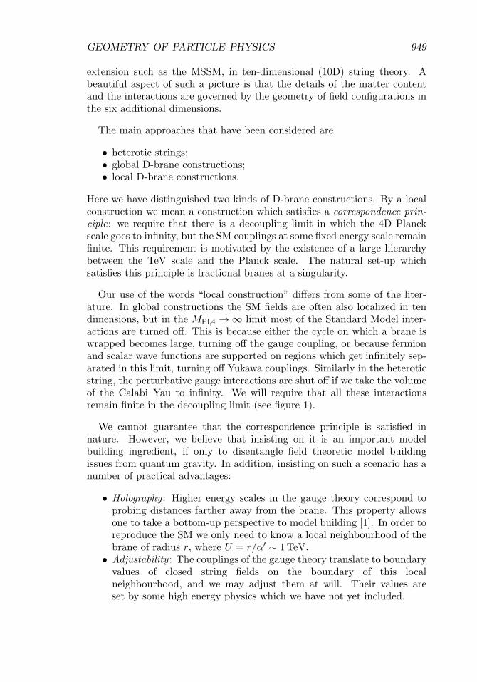
Our use of the words “local construction” differs from some of the liter-ature. In global constructions the SM fields are often also localized in tendimensions, but in the MPl,4 → ∞ limit most of the Standard Model inter-actions are turned off. This is because either the cycle on which a brane iswrapped becomes large, turning off the gauge coupling, or because fermionand scalar wave functions are supported on regions which get infinitely sep-arated in this limit, turning off Yukawa couplings. Similarly in the heteroticstring, the perturbative gauge interactions are shut off if we take the volumeof the Calabi–Yau to infinity. We will require that all these interactionsremain finite in the decoupling limit (see figure 1).
We cannot guarantee that the correspondence principle is satisfied innature. However, we believe that insisting on it is an important modelbuilding ingredient, if only to disentangle field theoretic model buildingissues from quantum gravity. In addition, insisting on such a scenario has anumber of practical advantages:
• Holography : Higher energy scales in the gauge theory correspond toprobing distances farther away from the brane. This property allowsone to take a bottom-up perspective to model building [1]. In order toreproduce the SM we only need to know a local neighbourhood of thebrane of radius r, where U = r/α′ ∼ 1 TeV.
• Adjustability : The couplings of the gauge theory translate to boundaryvalues of closed string fields on the boundary of this localneighbourhood, and we may adjust them at will. Their values areset by some high energy physics which we have not yet included.
950 MARTIJN WIJNHOLT
Figure 1: Caricature of a global D-brane model. If the size of the T 2 goesto infinity, as typically happens in the Mpl,4 → ∞ limit, the volumes of thebranes and the distance between their intersections goes to infinity as well,shutting of the Standard Model couplings.
• Uniqueness: It is expected that the closed string theory can be recov-ered from the open string theory. So up to some natural ambiguitieslike T-dualities, the local neighbourhood should be completely deter-mined by the ensemble of gauge theories obtained by varying the ranksof the gauge groups. Thus finding the local geometry for a gauge theoryis a relatively well-posed problem which should have a unique solution.The apparent non-uniqueness seen in other approaches is reflected herein the fact that there might be many different extensions of the samelocal geometry.
In [2] Herman Verlinde and the author gave a construction of a localmodel resembling the Minimal Supersymmetric Standard Model (MSSM).1
This construction had some drawbacks which could be traced back to thefact that we were working with oriented quivers. In this paper we addressthe problem of giving a local construction of the MSSM itself.
We have frequently seen the sentiment expressed that gauge theoriesobtained from branes at singularities are somehow rather special. Themain message of this paper is not so much that we can construct somespecific models. Rather it is that with the present set of ideas we can getpretty much any quiver gauge theory from branes at singularities. To illus-trate this point, we also engineer some classic models of dynamical SUSYbreaking.
While we touch on some more abstract topics like exceptional collections,the strategy is really very simple. We look for an embedding of the MSSM
1A closely related model was considered in [3].
GEOMETRY OF PARTICLE PHYSICS 951
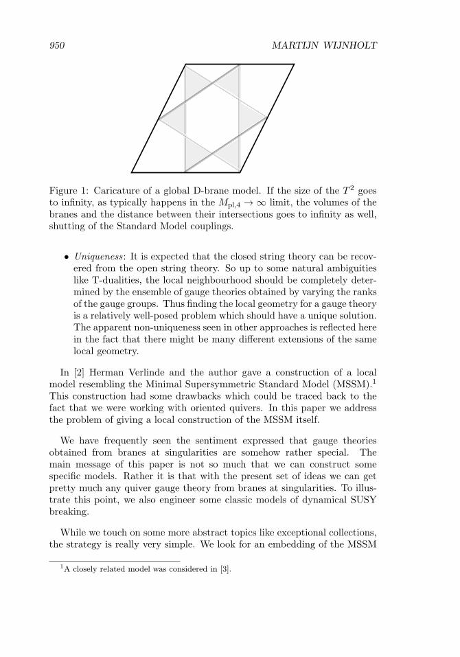
into a quiver gauge theory for which the geometric description is known, andthen turn on various vacuum expectation values (VEVs) and mass terms.In order to keep maximum control we require the deformations to preservesupersymmetry. Below the scale of the masses, we can effectively integrateout and forget the extra massive modes. On the geometric side, this corre-sponds to turning on certain moduli of the fractional brane or changing thecomplex structure of the singularity, and cutting off the geometry below thescale of the superfluous massive modes (see figure 2). Hence we can speakof the geometry of the MSSM.2
The Del Pezzo quiver and other intermediate quivers are purely auxiliarytheories which are possible UV extensions of the MSSM. Our constructionappears to be highly non-unique. This is a reflection of the bottom-upperspective, in which the theory can be extended in many ways beyond theTeV scale.
While we do not believe it is an issue, we should mention a possible caveatin our construction. As we will review we can vary superpotential terms inthe original Del Pezzo quiver independently,3 and it is expected but notcompletely obvious that the same is true in the Higgsed superpotential.One would like to prove that one can vary mass terms independently sothat we can keep some non-chiral Higgs fields light and the remainder arbi-trarily heavy. We checked on the computer in a number of simple examplesthat it works as expected. However, in our realistic examples some of themass terms in the Higgsed quiver should be induced from superpotentialterms in the original Del Pezzo quiver which are of 12th order in the fields.Unfortunately, due to memory constraints we have only been able to handlefourth and eighth order terms on the computer, and so we have not explic-itly shown in these examples that all excess non-chiral matter can be givena mass.
1.2 The MSSM as a quiver
Let us now describe what we mean by obtaining the MSSM. With D-branes,the best one can do is obtaining the MSSM together with an additionalmassive gauge boson. In addition, the right-handed neutrino sector is notset in stone. We first describe the quiver we would like to produce. In latersections, we describe how to engineer it.
2Recently some attempts have been made to construct such a geometry directly fromthe MSSM [4].
3This is a crucial difference with generic global D-brane models.

952 MARTIJN WIJNHOLT
Figure 2: The radial direction away from the fractional brane is interpretedas an energy scale. After Higgsing the Del Pezzo quiver theory, a sufficientlysmall neighbourhood of the singularity describes the MSSM.
Any weakly coupled4 D-brane construction of the MSSM will have at leastone extra massive gauge boson, namely gauged baryon number,5 becausethe SU(3)colour always gets enhanced to U(3). In addition, we have to choosehow to realize the right-handed neutrino sector. The most likely sources forright-handed neutrinos are:
(a) open strings charged with respect to a gauge symmetry that is notpart of the SM;
(b) uncharged open strings;(c) superpartners of closed string moduli.
Since all such modes are singlets under the observed low-energy gaugegroups, they will probably mix and there may not be an invariant distinctionbetween them.
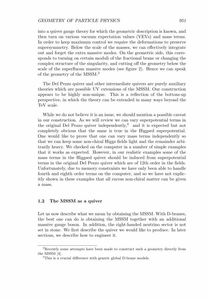
One of the closest quivers we could try to construct is shown in figure 3A.This is essentially the “four-stack” quiver first discussed in [5]. It consists ofthe MSSM plus U(1)B and U(1)L vector bosons, and a right-handed neutrinosector from charged open strings. Many groups have searched for this modeland closely related ones in specific compactifications, see for instance [6, 7]and the review [8].
4This conclusion can be evaded by using mutually non-local 7-branes in the construc-tion, that is by dropping the requirement that the dilaton is small near the 7-branes.
5It is possible to construct weakly coupled D-brane models in which the extra U(1)is not baryon number, e.g., by taking right-handed quarks to be in the 2-index anti-symmetric representation of SU(3). However, such models are problematic at the level ofinteractions and so will not be considered.
GEOMETRY OF PARTICLE PHYSICS 953
Figure 3: (A) An MSSM quiver, with an additional massless U(1)B−L. (B)Model I, a left-right unified model which can be Higgsed to the MSSM.
The combination U(1)B+L is anomalous, and as usual gets a mass bycoupling to a closed string axion (the Stuckelberg mechanism). Note thisis not the PQ axion, which may or may not exist, depending on the UVextension of the local geometry. The combination U(1)B−L is not anoma-lous, but could still get a mass by coupling to a closed string axion, alsodepending on the UV completion. However, if we take the gauge group onthe bottom node to be literally O(2), i.e., obtained from an orientifold pro-jection of U(2), then this O(2) cannot have a Stuckelberg coupling to anaxion. Since we would like to keep a massless U(1)Y , and since U(1)Y isa linear combination of the SO(2) and U(1)B−L, this means that U(1)B−L
cannot get a mass through the Stuckelberg mechanism.6
Thus we have two options. Either we instead construct the orientifoldmodel in figure 4, where the U(1) on the bottom node comes from identifyingtwo different nodes on the covering quiver. Then we have recourse to theStuckelberg mechanism to get rid of U(1)B−L. We will call this quiver modelII. A construction of this model is given in Section 4.3.
Alternatively we can make the extra U(1) massive by conventional Hig-gsing. This requires adding some non-chiral matter and condensing it, orturning on a VEV for a right-handed s-neutrino. In this case, we wouldfinally end up with the quiver in figure 5.7 This quiver consists of theMSSM, together with a massive U(1)B gauge boson, and a right-handedneutrino sector from uncharged open strings (adjoints).
6This agrees with [7], where all the O(2) models had a massless U(1)B−L.7The non-SUSY version of this quiver was recently discussed in [9].

954 MARTIJN WIJNHOLT
Figure 4: Model II: a quiver consisting of the MSSM, U(1)B−L plus a mas-sive U(1)B+L. The U(1)B−L can be coupled to a Stuckelberg field.
Figure 5: The Standard Model plus U(1)B. Note we still need R-parity toforbid undesirable couplings.
If in fact we use the second option, adding non-chiral matter and Higgsing,then for our purposes here we might as well replace the O(2) with a USp(2),since both break to the same model up to some massive particles. In thelocal set-up, the masses of the extra particles may be taken arbitrarily large.Moreover, up to the massive U(1)B this is actually a well-known unifiedmodel, the minimal left–right symmetric model (an intermediate step toSO(10) unification), so it has some independent interest. Thus we mightas well construct the quiver in figure 3B, which we will call model I. Thisis the simpler of the constructions in this paper, and will be explained inSection 4.1.
We should point out that R-parity is not quite automatic in either of ourmodels, although both models appear to have a global U(1)B−L. In ourfirst model we must preserve R-parity in our final Higgsing to the MSSM.In both models we might need to worry about D-instanton effects which
GEOMETRY OF PARTICLE PHYSICS 955
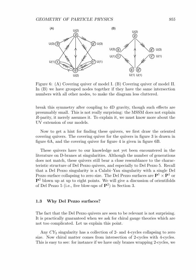
Figure 6: (A) Covering quiver of model I. (B) Covering quiver of model II.In (B) we have grouped nodes together if they have the same intersectionnumbers with all other nodes, to make the diagram less cluttered.
break this symmetry after coupling to 4D gravity, though such effects arepresumably small. This is not really surprising: the MSSM does not explainR-parity, it merely assumes it. To explain it, we must know more about theUV extension of our models.
Now to get a hint for finding these quivers, we first draw the orientedcovering quivers. The covering quiver for the quivers in figure 3 is drawn infigure 6A, and the covering quiver for figure 4 is given in figure 6B.
These quivers have to our knowledge not yet been encountered in theliterature on D-branes at singularities. Although the number of generationsdoes not match, these quivers still bear a close resemblance to the charac-teristic structure of Del Pezzo quivers, and especially to Del Pezzo 5. Recallthat a Del Pezzo singularity is a Calabi–Yau singularity with a single DelPezzo surface collapsing to zero size. The Del Pezzo surfaces are P1 × P1 orP2 blown up at up to eight points. We will give a discussion of orientifoldsof Del Pezzo 5 (i.e., five blow-ups of P2) in Section 3.
1.3 Why Del Pezzo surfaces?
The fact that the Del Pezzo quivers are seen to be relevant is not surprising.It is practically guaranteed when we ask for chiral gauge theories which arenot too complicated. Let us explain this point.
Any CY3 singularity has a collection of 2- and 4-cycles collapsing to zerosize. Now chiral matter comes from intersection of 2-cycles with 4-cycles.This is easy to see: for instance if we have only branes wrapping 2-cycles, we
956 MARTIJN WIJNHOLT
can always deform the branes (at some cost in energy) so that they do notintersect. Then all open string modes are massive, and thus the net numberof chiral fermions must be zero. So requiring chiral fermions implies thatwe have to have some collapsing 4-cycles in the geometry. The Del Pezzosingularities, which have precisely a single collapsing 4-cycle, are then thesimplest examples.
Moreover, a minimal D-brane realization of the SM has one local U(1)which is anomalous, namely U(1)B, and this lifts to two anomalous U(1)’son the oriented covering quiver. Now the the number of anomalous U(1)’sis interpreted geometrically as the rank of the intersection matrix of vanish-ing cycles. Hence the Del Pezzo quivers and their orientifolds are naturalcandidates because they are chiral quivers with the minimum number ofanomalous U(1)’s, namely two.
Although the models we are looking for are not among the known DelPezzo quivers, these arguments convinced us that we should derive themfrom the quivers that were already known, rather than look for new singu-larities.
2 Lightning review of branes at singularities
Consider a Calabi–Yau singularity in IIb string theory, characterized by acollection of vanishing 2- and 4-cycles. Since the curvature is very large, it isin general not clear how to define the notion of a D-brane at a singularity. Annotable exception is the case of orbifold singularities, where we can use freefield theory. From this special case the following picture has emerged: givena singularity we expect the existence of a finite set of irreducible “fractional”branes. For the case of orbifolds these irreducible branes are in one-to-onecorrespondence with the irreducible representation of the orbifold group.To these irreducible branes we can associate the basic quiver diagram. Foreach irreducible fractional brane we draw a node, and for each masslessopen string which goes from brane i to brane j we draw an arrow or anedge between the corresponding nodes. All the remaining branes can beexpressed as bound states of these irreducible branes, or equivalently as aHiggsing of the basic quiver.
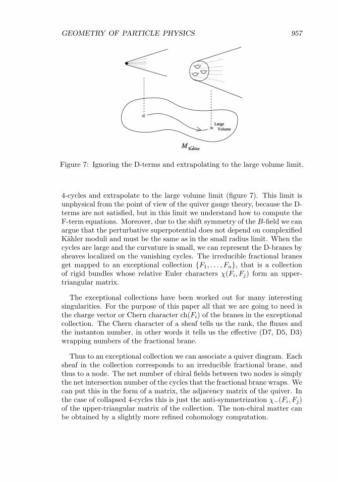
Now how do we find the basic quiver for a general singularity? Let usassume our branes are half BPS and space–time filling, so that we get a4D N = 1 quiver gauge theory. Then we can use the following strategy:we make sure that the F-term equations are satisfied, but we temporarilyignore the D-term equations. Then we can blow up the vanishing 2- and
GEOMETRY OF PARTICLE PHYSICS 957
Figure 7: Ignoring the D-terms and extrapolating to the large volume limit.
4-cycles and extrapolate to the large volume limit (figure 7). This limit isunphysical from the point of view of the quiver gauge theory, because the D-terms are not satisfied, but in this limit we understand how to compute theF-term equations. Moreover, due to the shift symmetry of the B-field we canargue that the perturbative superpotential does not depend on complexifiedKahler moduli and must be the same as in the small radius limit. When thecycles are large and the curvature is small, we can represent the D-branes bysheaves localized on the vanishing cycles. The irreducible fractional branesget mapped to an exceptional collection {F1, . . . , Fn}, that is a collectionof rigid bundles whose relative Euler characters χ(Fi, Fj) form an upper-triangular matrix.
The exceptional collections have been worked out for many interestingsingularities. For the purpose of this paper all that we are going to need isthe charge vector or Chern character ch(Fi) of the branes in the exceptionalcollection. The Chern character of a sheaf tells us the rank, the fluxes andthe instanton number, in other words it tells us the effective (D7, D5, D3)wrapping numbers of the fractional brane.
Thus to an exceptional collection we can associate a quiver diagram. Eachsheaf in the collection corresponds to an irreducible fractional brane, andthus to a node. The net number of chiral fields between two nodes is simplythe net intersection number of the cycles that the fractional brane wraps. Wecan put this in the form of a matrix, the adjacency matrix of the quiver. Inthe case of collapsed 4-cycles this is just the anti-symmetrization χ−(Fi, Fj)of the upper-triangular matrix of the collection. The non-chiral matter canbe obtained by a slightly more refined cohomology computation.
958 MARTIJN WIJNHOLT
As mentioned we can also reconstruct other F-term data such as thesuperpotential. The physicists method is to compute some correlation func-tions of the chiral fields. The mathematicians method is to first compute thedual exceptional collection, whose relative Euler characters are given by theinverse of the above-mentioned upper-triangular matrix. The superpotentialnow follows from the relations in the path algebra of the dual collection.
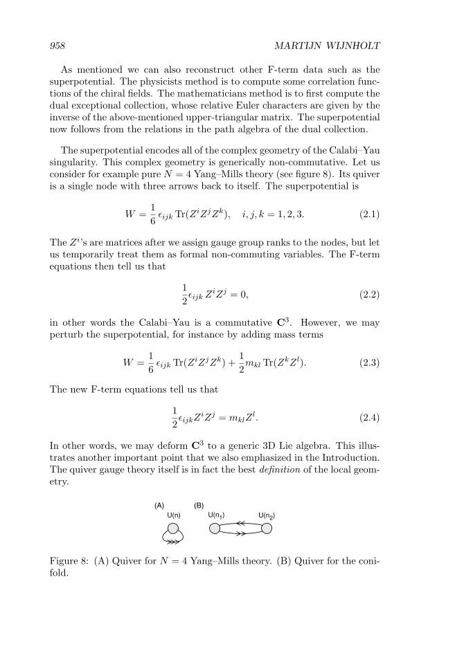
The superpotential encodes all of the complex geometry of the Calabi–Yausingularity. This complex geometry is generically non-commutative. Let usconsider for example pure N = 4 Yang–Mills theory (see figure 8). Its quiveris a single node with three arrows back to itself. The superpotential is
W =16
εijk Tr(ZiZjZk), i, j, k = 1, 2, 3. (2.1)
The Zi’s are matrices after we assign gauge group ranks to the nodes, but letus temporarily treat them as formal non-commuting variables. The F-termequations then tell us that
12εijk ZiZj = 0, (2.2)
in other words the Calabi–Yau is a commutative C3. However, we mayperturb the superpotential, for instance by adding mass terms
W =16
εijk Tr(ZiZjZk) +12mkl Tr(ZkZ l). (2.3)
The new F-term equations tell us that
12εijkZ
iZj = mklZl. (2.4)
In other words, we may deform C3 to a generic 3D Lie algebra. This illus-trates another important point that we also emphasized in the Introduction.The quiver gauge theory itself is in fact the best definition of the local geom-etry.
Figure 8: (A) Quiver for N = 4 Yang–Mills theory. (B) Quiver for the coni-fold.
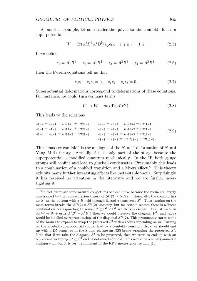
GEOMETRY OF PARTICLE PHYSICS 959
As another example, let us consider the quiver for the conifold. It has asuperpotential
W = Tr(AiBkAjBl) εijεkl, i, j, k, l = 1, 2. (2.5)
If we define
z1 = A1B1, z2 = A1B2, z3 = A2B1, z4 = A2B2, (2.6)
then the F-term equations tell us that
zizj − zjzi = 0, z1z4 − z2z3 = 0. (2.7)
Superpotential deformations correspond to deformations of these equations.For instance, we could turn on mass terms
W → W + mij Tr(AiBj). (2.8)
This leads to the relations
z1z2 − z2z1 = m21z1 + m22z2, z2z3 − z3z2 = m22z4 − m11z1,z3z1 − z1z3 = m12z1 + m22z3, z2z4 − z4z2 = m11z2 + m21z4,z1z4 − z4z1 = m12z2 − m21z3, z4z3 − z3z4 = m11z3 + m12z4,
z1z4 − z2z3 = −m11z1 − m12z2.
(2.9)
This “massive conifold” is the analogue of the N = 1∗ deformation of N = 4Yang–Mills theory. Actually this is only part of the story, because thesuperpotential is modified quantum mechanically. In the IR both gaugegroups will confine and lead to glueball condensates. Presumably this leadsto a combination of a conifold transition and a Myers effect.8 This theoryexhibits many further interesting effects like meta-stable vacua. Surprisinglyit has received no attention in the literature and we are further inves-tigating it.
8In fact, there are some natural conjectures one can make because the vacua are largelyconstrained by the representation theory of SU(2) × SU(2). Classically, the conifold hasan S2 at the bottom with a B-field through it, and a transverse S3. Then turning on themass terms breaks the SU(2) × SU(2) isometry, but for certain masses there is a linearcombination corresponding to some S2 ⊂ P1 × P1 which is preserved. E.g., if we turnon W → W + m Tr(A1B2 − A2B1) then we would preserve the diagonal P1, and vacuawould be labelled by representations of the diagional SU(2). This presumably causes someof the branes to expand to wrap the preserved S2 with a radius depending on m. Turningon the glueball superpotential should lead to a conifold transition. Now we should endup with a D5-brane, or in the S-dual picture an NS5-brane wrapping the preserved S2.Note that if we take the diagonal S2 to be preserved, then we seem to end up with anNS5-brane wrapping S2 ⊂ S3 on the deformed conifold. This would be a supersymmetricconfiguration but it is very reminiscent of the KPV meta-stable vacuum [10].
960 MARTIJN WIJNHOLT
More generally, we will be interested in adding irrelevant terms to thesuperpotential. These clearly correspond to subleading complex structuredeformations of the singularity.
The physical intuition is that closed string modes are in one-to-one cor-respondence with general gauge invariant deformations of the quiver. Forsuperpotential deformations this has been put on a firm footing byKontsevich [11], who shows that infinitesimal deformations of the “derivedcategory” (i.e., single trace superpotential deformations) correspond toobservables in the closed string B-model. In the context of mirror sym-metry, the significance of this statement is that together with a correspond-ing statement for the A-model, it provides evidence for the correspondenceprinciple, i.e., the idea that classical mirror symmetry can be recovered fromhomological mirror symmetry.
As we explained, our main interest will be in the Del Pezzo quivers.The first five Del Pezzo quivers were found using orbifold and toric tech-niques [12–16]. Some of these were rederived using exceptional collectionsin [17,18], and finally the remaining five non-toric Del Pezzo quivers, includ-ing Del Pezzo 5 which will play a central role in this paper, were foundusing exceptional collections [19]. We refer to [19, 20] for more detailedreviews and explicit computations. For other interesting works we referto [21–25].
3 Orientifolding quivers
Discussions of orientifolds and derived categories have recently been givenin the LG regime [26] and in the large volume regime [27]. Here we describeorientifolds in another regime, which is captured by quiver gauge theories.Traditionally orientifolds of branes at singularities have been derived by firstspecifying an orientifold action on the closed string modes, and then findingthe induced action on open string modes. Here we start by specifying anorientifold action on the open string modes. This simplifies the task offinding a brane realization of a desired gauge theory, and at any rate theclosed string geometry can be reconstructed from the gauge theory.
3.1 General discussion of orientifolding
Perturbative string theory on IIb backgrounds has a number of Z2 symme-tries. They include (−1)FL and worldsheet parity P . In addition, on a givenbackground the theory may have an additional Z2 symmetry σ.
GEOMETRY OF PARTICLE PHYSICS 961
Given such a symmetry, we can construct a new perturbative string back-ground by gauging it. An orientifold projection is an orbifold which involvesP . In addition, we would like to preserve N = 1 SUSY in four dimensions.Recall that in IIB string theory on a Calabi–Yau the supercharges withpositive 4D chirality are derived from the currents
j1α = e−ϕL/2 SLα e
12
∫JL , j2
α = e−ϕR/2 SRα e12
∫JR , (3.1)
where in the large volume limit
e∫
JL = Ω(3,0)ijk ψi
LψjLψk
L, e∫
JR = Ω(3,0)ijk ψi
RψjRψk
R. (3.2)
We have used the conventional notations for the bosonized superghost, 4Dspin fields and wordsheet fermions. In type IIa, the second current wouldhave been proportional to the square root of Ω(0,3)
ijkψi
RψjRψk
R, because thesecond spinor must have negative 10D chirality. In order to preserve SUSYthere must be a linear combination that is preserved. If we do not include(−1)FL , then
Q1α + Q2
α (3.3)
is preserved under orientifolding, provided σ is a symmetry of the internalCFT that maps Ω(3,0) → Ω(3,0). If we instead include (−1)FL in the orien-tifolding, then
Q1α − iQ2
α (3.4)
is preserved under orientifolding, provided σ maps Ω(3,0) → −Ω(3,0).
Parity exchanges the Chan–Paton factors at the ends of an open string,and acts as −1 on massless open string modes, so it maps gauge fields andchiral fields to minus their transpose. We are interested in local orientifoldmodels, so we will be looking for symmetries of the quiver of irreduciblebranes which map a gauge field at node i to minus the transpose of thegauge field at some node j, and map any chiral field X to the transpose Y T
of some other chiral field, possibly up to an additional gauge transformationwhich we call γ. We denote this as i ↔ j∗. In our decoupling limit, findingsuch a symmetry is sufficient, because the irreducible branes generate allother branes and closed strings ought to be recovered from open strings.In particular, we can read of the local geometry from the gauge invariantoperators and their relations.
We will assume canonical kinetic terms for the chiral fields, so we canactually map X → eiϕY T for some phase ϕ. If there are multiple arrows
962 MARTIJN WIJNHOLT
between two nodes, we can upgrade the map to a unitary matrix. In order topreserve SUSY, the orientifold action has to leave the superspace coordinateθ invariant, and hence it will also have to leave the superpotential invariant.This may lead to correlations between the SO and Sp projections on differentnodes, and symmetric or anti-symmetric projections on chiral fields that aremapped to themselves.
One should keep in mind that a non-anomalous quiver theory may becomeanomalous after projection if the ranks of the gauge groups are not adjusted.The orientifold may project out more of the positive than of the negative con-tributions to an anomaly. This is generically the case if the projected theorycontains symmetric and anti-symmetric tensor matter. From the geometricpoint of view, this is because an orientifold plane may give additional tad-pole contributions, which need to be cancelled by adding additional branes,i.e., adjusting the ranks of the gauge groups.
We can also understand how the orientifold acts on closed string modes.The modes that are kept are simply the closed string modes on the coverthat can be used to deform the orientifolded theory. To preserve SUSY,the orientifold action maps τi → τj∗ and Li → −Lj∗ , where τ denotes thecomplexified gauge coupling and L denotes the linear multiplet containingthe FI parameter and the Stuckelberg 2-form field.
3.2 Examples
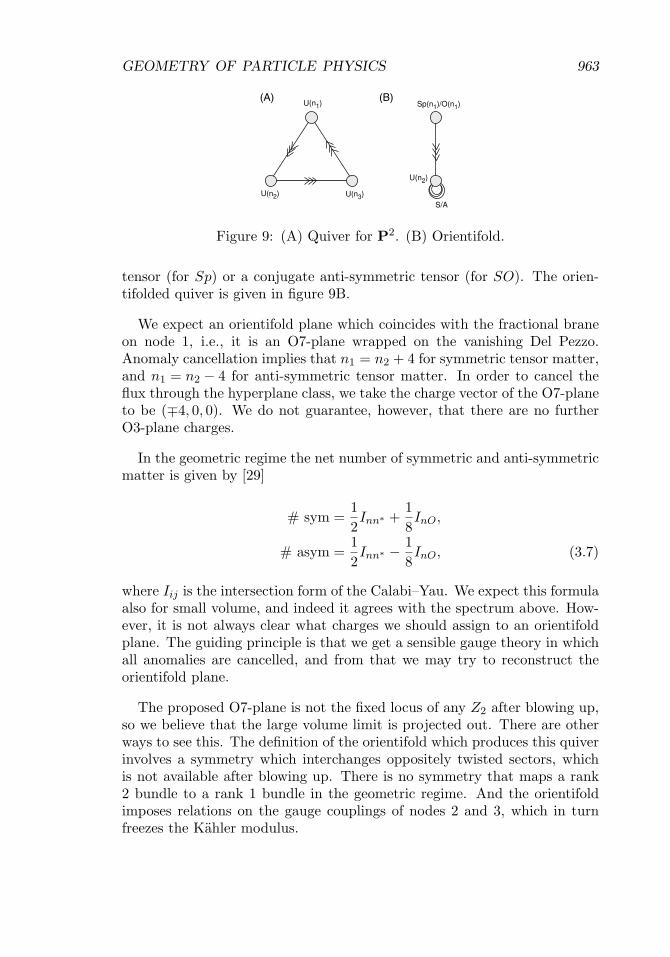
Orientifold of P2
The simplest case to understand is the Calabi–Yau cone over P2, which isidentical to the orbifold singularity C3/Z3. This orientifold is already knownin the literature [28], but we will use a slightly more geometric perspective.We denote the hyperplane class by H. The quiver is given in figure 9A andmay be obtained from a set of fractional branes with the following (D7, D5,D3) wrapping numbers:
1. (1, 0, 0) 2. −(
2, H, −12
)3.
(1, H,
12
). (3.5)
We consider the following symmetry:
1 ↔ 1∗, 2 ↔ 3∗. (3.6)
We may take an Sp- or SO-projection. Assuming the usual orbifold superpo-tential, the matter between nodes 2 and 3 projects to a conjugate symmetric
GEOMETRY OF PARTICLE PHYSICS 963
Figure 9: (A) Quiver for P2. (B) Orientifold.
tensor (for Sp) or a conjugate anti-symmetric tensor (for SO). The orien-tifolded quiver is given in figure 9B.
We expect an orientifold plane which coincides with the fractional braneon node 1, i.e., it is an O7-plane wrapped on the vanishing Del Pezzo.Anomaly cancellation implies that n1 = n2 + 4 for symmetric tensor matter,and n1 = n2 − 4 for anti-symmetric tensor matter. In order to cancel theflux through the hyperplane class, we take the charge vector of the O7-planeto be (∓4, 0, 0). We do not guarantee, however, that there are no furtherO3-plane charges.
In the geometric regime the net number of symmetric and anti-symmetricmatter is given by [29]
# sym =12Inn∗ +
18InO,
# asym =12Inn∗ − 1
8InO, (3.7)
where Iij is the intersection form of the Calabi–Yau. We expect this formulaalso for small volume, and indeed it agrees with the spectrum above. How-ever, it is not always clear what charges we should assign to an orientifoldplane. The guiding principle is that we get a sensible gauge theory in whichall anomalies are cancelled, and from that we may try to reconstruct theorientifold plane.
The proposed O7-plane is not the fixed locus of any Z2 after blowing up,so we believe that the large volume limit is projected out. There are otherways to see this. The definition of the orientifold which produces this quiverinvolves a symmetry which interchanges oppositely twisted sectors, whichis not available after blowing up. There is no symmetry that maps a rank2 bundle to a rank 1 bundle in the geometric regime. And the orientifoldimposes relations on the gauge couplings of nodes 2 and 3, which in turnfreezes the Kahler modulus.
964 MARTIJN WIJNHOLT
The case of the SO projection with n2 = 5 gives us a simple 3-generationSU(5) GUT with a 5 and a 10 from the anti-symmetric [28]. There are noHiggses, though they could presumably be generated by first increasing theranks and then Higgsing. Of course, there would be well-known problemswith getting the 5 × 10 × 10 Yukawa’s. This model also exhibits dynamicalSUSY breaking [28], but with a runaway behaviour.
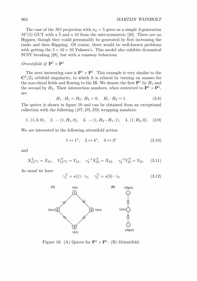
Orientifold of P1 × P1
The next interesting case is P1 × P1. This example is very similar to theC3/Z4 orbifold singularity, to which it is related by turning on masses forthe non-chiral fields and flowing to the IR. We denote the first P1 by H1 andthe second by H2. Their intersection numbers, when restricted to P1 × P1,are
H1 · H1 = H2 · H2 = 0, H1 · H2 = 1. (3.8)The quiver is shown in figure 10 and can be obtained from an exceptionalcollection with the following (D7, D5, D3) wrapping numbers:
1. (1, 0, 0), 2. − (1, H1, 0), 3. − (1, H2−H1, 1), 4. (1, H2, 0). (3.9)
We are interested in the following orientifold action:
1 ↔ 1∗, 2 ↔ 4∗, 3 ↔ 3∗ (3.10)
and
XT12γ1 = X41, Y T
12γ1 = Y41, γ−13 XT
23 = X34, γ−13 Y T
23 = Y34. (3.11)
As usual we haveγT
1 = s(1) · γ1, γT3 = s(3) · γ3 (3.12)
Figure 10: (A) Quiver for P1 × P1. (B) Orientifold.
GEOMETRY OF PARTICLE PHYSICS 965
with s = ±1, in order for the action on the gauge fields to be an involution.The superpotential of the commutative P1 × P1 quiver is
W = X12X23X34X41 − X12Y23X34Y41 + Y12Y23Y34Y41 − Y12X23Y34X41.(3.13)
In order for this particular superpotential to be invariant, we also need
s(1) · s(3) = +1, (3.14)
so we can have an SO/SO or an Sp/Sp projection. More generally we couldwork the other way around. We first decide on the projections that wewould like to have, and then we write down the most general superpotentialcompatible with those projections.
The orientifold locus appears to consist of the union of two O7-planes,with wrapping numbers 4(1, 0, 0) and −4(1, H2−H1, 1). This is not thefixed locus of any Z2 symmetry after blowing up, so the large volume limitis projected out.
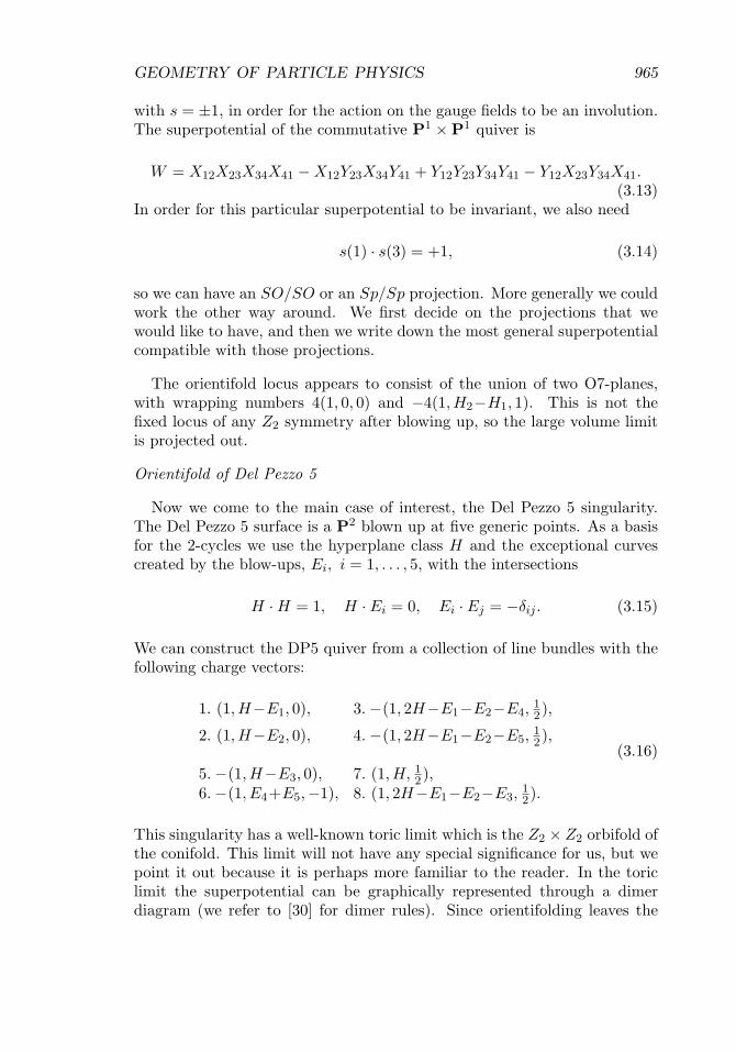
Orientifold of Del Pezzo 5
Now we come to the main case of interest, the Del Pezzo 5 singularity.The Del Pezzo 5 surface is a P2 blown up at five generic points. As a basisfor the 2-cycles we use the hyperplane class H and the exceptional curvescreated by the blow-ups, Ei, i = 1, . . . , 5, with the intersections
H · H = 1, H · Ei = 0, Ei · Ej = −δij . (3.15)
We can construct the DP5 quiver from a collection of line bundles with thefollowing charge vectors:
1. (1, H−E1, 0), 3. −(1, 2H−E1−E2−E4,12),
2. (1, H−E2, 0), 4. −(1, 2H−E1−E2−E5,12),
5. −(1, H−E3, 0), 7. (1, H, 12),
6. −(1, E4+E5,−1), 8. (1, 2H−E1−E2−E3,12).
(3.16)
This singularity has a well-known toric limit which is the Z2 × Z2 orbifold ofthe conifold. This limit will not have any special significance for us, but wepoint it out because it is perhaps more familiar to the reader. In the toriclimit the superpotential can be graphically represented through a dimerdiagram (we refer to [30] for dimer rules). Since orientifolding leaves the
966 MARTIJN WIJNHOLT
superpotential invariant, it must correspond to a reflection or 180◦ degreerotation of the dimer. The toric superpotential is read off to be:
W = X13X35X58X81 − X14X46X68X81 + X14X45X57X71
− X13X36X67X71 + X24X46X67X72 − X23X35X57X72
+ X23X36X68X82 − X24X45X58X82 (3.17)
and it is invariant under the reflection in the axis indicated in figure 11.
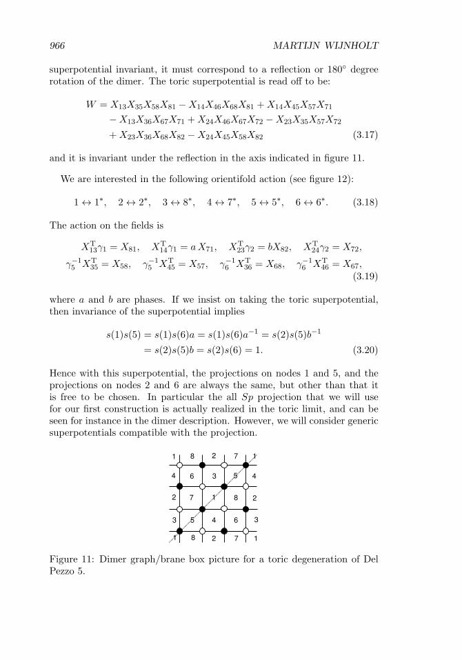
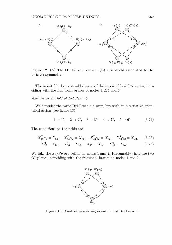
We are interested in the following orientifold action (see figure 12):
1 ↔ 1∗, 2 ↔ 2∗, 3 ↔ 8∗, 4 ↔ 7∗, 5 ↔ 5∗, 6 ↔ 6∗. (3.18)
The action on the fields is
XT13γ1 = X81, XT
14γ1 = a X71, XT23γ2 = bX82, XT
24γ2 = X72,
γ−15 XT
35 = X58, γ−15 XT
45 = X57, γ−16 XT
36 = X68, γ−16 XT
46 = X67,(3.19)
where a and b are phases. If we insist on taking the toric superpotential,then invariance of the superpotential implies
s(1)s(5) = s(1)s(6)a = s(1)s(6)a−1 = s(2)s(5)b−1
= s(2)s(5)b = s(2)s(6) = 1. (3.20)
Hence with this superpotential, the projections on nodes 1 and 5, and theprojections on nodes 2 and 6 are always the same, but other than that itis free to be chosen. In particular the all Sp projection that we will usefor our first construction is actually realized in the toric limit, and can beseen for instance in the dimer description. However, we will consider genericsuperpotentials compatible with the projection.
Figure 11: Dimer graph/brane box picture for a toric degeneration of DelPezzo 5.
GEOMETRY OF PARTICLE PHYSICS 967
Figure 12: (A) The Del Pezzo 5 quiver. (B) Orientifold associated to thetoric Z2 symmetry.
The orientifold locus should consist of the union of four O7-planes, coin-ciding with the fractional branes of nodes 1, 2, 5 and 6.
Another orientifold of Del Pezzo 5
We consider the same Del Pezzo 5 quiver, but with an alternative orien-tifold action (see figure 13)
1 → 1∗, 2 → 2∗, 3 → 8∗, 4 → 7∗, 5 → 6∗. (3.21)
The conditions on the fields are
XT13γ1 = X81, XT
14γ2 = X71, XT23γ2 = X82, XT
24γ2 = X72, (3.22)
XT35 = X68, XT
36 = X58, XT45 = X67, XT
46 = X57. (3.23)
We take the Sp/Sp projection on nodes 1 and 2. Presumably there are twoO7-planes, coinciding with the fractional branes on nodes 1 and 2.
Figure 13: Another interesting orientifold of Del Pezzo 5.
968 MARTIJN WIJNHOLT
Figure 14: Quiver for Del Pezzo 7.
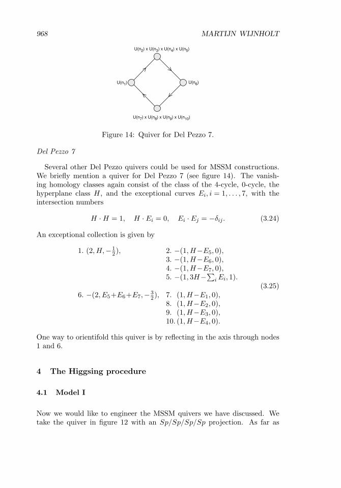
Del Pezzo 7
Several other Del Pezzo quivers could be used for MSSM constructions.We briefly mention a quiver for Del Pezzo 7 (see figure 14). The vanish-ing homology classes again consist of the class of the 4-cycle, 0-cycle, thehyperplane class H, and the exceptional curves Ei, i = 1, . . . , 7, with theintersection numbers
H · H = 1, H · Ei = 0, Ei · Ej = −δij . (3.24)
An exceptional collection is given by
1. (2, H, −12), 2. −(1, H−E5, 0),
3. −(1, H−E6, 0),4. −(1, H−E7, 0),5. −(1, 3H−
∑i Ei, 1).
6. −(2, E5+E6+E7,−32), 7. (1, H−E1, 0),
8. (1, H−E2, 0),9. (1, H−E3, 0),10. (1, H−E4, 0).
(3.25)
One way to orientifold this quiver is by reflecting in the axis through nodes1 and 6.
4 The Higgsing procedure
4.1 Model I
Now we would like to engineer the MSSM quivers we have discussed. Wetake the quiver in figure 12 with an Sp/Sp/Sp/Sp projection. As far as
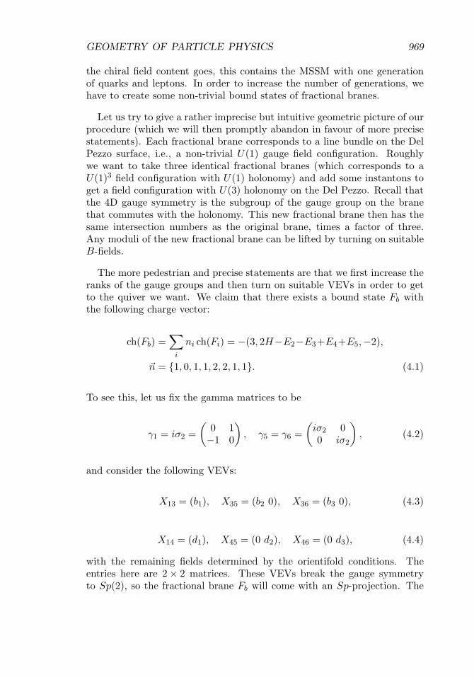
GEOMETRY OF PARTICLE PHYSICS 969
the chiral field content goes, this contains the MSSM with one generationof quarks and leptons. In order to increase the number of generations, wehave to create some non-trivial bound states of fractional branes.
Let us try to give a rather imprecise but intuitive geometric picture of ourprocedure (which we will then promptly abandon in favour of more precisestatements). Each fractional brane corresponds to a line bundle on the DelPezzo surface, i.e., a non-trivial U(1) gauge field configuration. Roughlywe want to take three identical fractional branes (which corresponds to aU(1)3 field configuration with U(1) holonomy) and add some instantons toget a field configuration with U(3) holonomy on the Del Pezzo. Recall thatthe 4D gauge symmetry is the subgroup of the gauge group on the branethat commutes with the holonomy. This new fractional brane then has thesame intersection numbers as the original brane, times a factor of three.Any moduli of the new fractional brane can be lifted by turning on suitableB-fields.
The more pedestrian and precise statements are that we first increase theranks of the gauge groups and then turn on suitable VEVs in order to getto the quiver we want. We claim that there exists a bound state Fb withthe following charge vector:
ch(Fb) =∑
i
ni ch(Fi) = −(3, 2H−E2−E3+E4+E5,−2),
�n = {1, 0, 1, 1, 2, 2, 1, 1}. (4.1)
To see this, let us fix the gamma matrices to be
γ1 = iσ2 =(
0 1−1 0
), γ5 = γ6 =
(iσ2 00 iσ2
), (4.2)
and consider the following VEVs:
X13 = (b1), X35 = (b2 0), X36 = (b3 0), (4.3)
X14 = (d1), X45 = (0 d2), X46 = (0 d3), (4.4)
with the remaining fields determined by the orientifold conditions. Theentries here are 2 × 2 matrices. These VEVs break the gauge symmetryto Sp(2), so the fractional brane Fb will come with an Sp-projection. The

970 MARTIJN WIJNHOLT
D-term equations may be satisfied by taking
15b1 =
14b2 =
13b3 =
(χ1 00 χ1
),
15d1 =
14d2 =
13d3 =
(χ2 00 χ2
). (4.5)
Clearly we need both quartic and octic terms in the superpotential, in orderto get mass terms for the adjoints associated with a rescaling of the VEVs.With such a superpotential, tuned so that the F-term equations are satisfiedand so that the orientifold symmetry is preserved, but otherwise generic, wefind that our bound state is rigid, i.e., it has no massless adjoints.
We also claim that there exists a bound state Fa with the following chargevector:9
ch(Fa) =∑
i
ni ch(Fi) = (3, 2H−E1−E2+E4+E5, 0),
�n = {2, 2, 1, 1, 1, 0, 1, 1}. (4.6)
This is very similar to Fb so we do not need to repeat the analysis. Thefractional brane Fa also inherits an Sp projection.
Next we compute the massless fields in the quiver for {2Fa, 3F3, F4, 2Fb,F7, 3F8}. For a generic superpotential (apart from the conditions men-tioned above) we found that the spectrum is completely chiral, as shownin figure 15. This quiver is a Higgsed version of the original Del Pezzoquiver. It inherits the following orientifold projection:
XiTa3 γa = Xi
8a, XiTa4 γa = Xi
7a, γ−1b XiT
3b = Xib8,
γ−1b XiT
4b = Xib7, i = 1, 2, 3. (4.7)
Moreover, we expect to be able to get a generic superpotential for this quiverprovided we included sufficiently many higher order terms in the original DelPezzo quiver. Checking we can get generic fourth and eighth-order terms iscomputationally too intensive, so we will assume it from now on.
This is almost what we want. After orientifolding we get all the chiralfields of the MSSM. However, we also want some non-chiral matter: theconventional Higgses Hu, Hd and the additional Higgs fields which breakSp(2)R × U(1)L → U(1). This cannot be obtained by tuning the originalbound state/superpotential, because the candidate non-chiral fields are infact eaten by gauge bosons. So we create a new quiver with the same chiral
9This charge vector is probably not the Chern character of a sheaf; instead it shouldbe interpreted as a bound state of branes and ghost branes in the large volume limit [20].
GEOMETRY OF PARTICLE PHYSICS 971
Figure 15: Intermediate quiver.
matter content, but with more candidate non-chiral fields.10 To do this wereplace Fb by the bound state Fd with charge vector
ch(Fd) = ch(Fa) + ch(F3) + 2 ch(Fb) + ch(F8)
= −(3, 2H + E1 − E2 − E3 + E5,−4). (4.8)
This can be done for instance by turning on VEVs of the following form:
X1a4 = (s1), X1
4b = (s2 0), X24b = (0 s3) (4.9)
and the remaining non-zero VEVs fixed by the orientifold conditions. Wecan satisfy the D-terms by setting
15s1 =
14s2 =
13s3 =
(φ 00 φ
). (4.10)
In order for this to satisfy the F-term equations, and to get the desiredmassless non-chiral matter, we have to impose some restrictions on thesuperpotential. If we use both quartic and octic terms, one can lift all thenon-chiral matter and the quiver generated by {2Fa, 3F3, F4, 2Fd, F7, 3F8}is the same as in figure 15 again. However, now there are two non-chiralpairs between Fa and Fd and two non-chiral pairs between Fd and F4/F7.We have checked that the superpotential can be tuned so that one of eachof these pairs becomes light, and so we end up with the required quiver infigure 6A.
10Alternatively, we could use more complicated bound states from the beginning, butthen we would have to work with superpotential terms of order 12 or higher in order tolift the excess non-chiral matter.
972 MARTIJN WIJNHOLT
4.2 Pati–Salam
The quiver we have obtained above also gives a three-generation SUSY Pati–Salam model, by changing the ranks of the gauge groups (U(3) → U(0), andU(1) → U(4)).
Very similar tricks may also be applied to the P1 × P1 quiver to constructPati–Salam models, though in that case the number of generations will beeven. Let us show how we can obtain a four-generation Pati-Salam model.We define the gamma matrices as
γ1 =(
0 1−1 0
), γ3 =
(0 13×3
−13×3 0
). (4.11)
Then we construct a bound state Fb with charge vector
ch(Fb) = ch(F1) + 2ch(F2) + 3ch(F3) + 2ch(F4) = −(2, H2−H1, 3) (4.12)
by turning on the following VEVs:
X12 =(
a1 0 0 00 0 a1 0
), Y12 =
(0 a1 0 00 0 0 a1
), (4.13)
X23 =
⎛⎜⎜⎝
a2 0 0 0 0 00 0 a3 0 0 00 0 0 a2 0 00 0 0 0 0 a3
⎞⎟⎟⎠ , Y23 =
⎛⎜⎜⎝
0 0 0 0 0 00 a4 0 0 0 00 0 0 0 0 00 0 0 0 a4 0
⎞⎟⎟⎠ (4.14)
with the remaining VEVs determined by the orientifold symmetry. TheD-terms are satisfied if we pick
a1 = a2 = 5ψ, a3 = 4ψ, a4 = 3ψ. (4.15)
Similarly, we construct a bound state Fa with charge vector
ch(Fa) = 3ch(F1) + 2ch(F2) + ch(F3) + 2ch(F4) = (2, H2−H1,−1). (4.16)
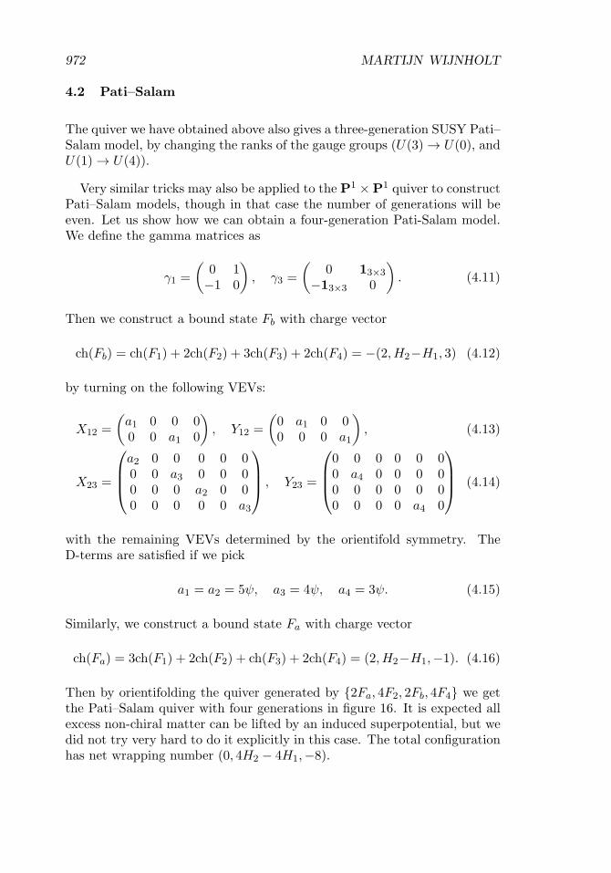
Then by orientifolding the quiver generated by {2Fa, 4F2, 2Fb, 4F4} we getthe Pati–Salam quiver with four generations in figure 16. It is expected allexcess non-chiral matter can be lifted by an induced superpotential, but wedid not try very hard to do it explicitly in this case. The total configurationhas net wrapping number (0, 4H2 − 4H1,−8).
GEOMETRY OF PARTICLE PHYSICS 973
Figure 16: A four-generation Pati-Salam model from P1 × P1.
4.3 Model II
We now consider an alternative construction, in which U(1)B−L can get amass through the Stuckelberg mechanism (depending on the UV completion[31]).
The orientifold projection is as in (3.21). We would like to form thefollowing bound states:
ch(Fa) =∑
i
ni ch(Fi) = (3, 2H−2E1+E2−E3+E4+E5, 1),
�na = {4, 1, 2, 2, 1, 1, 2, 2},
ch(Fb) =∑
i
ni ch(Fi) = −(3,−E1−2E2+3E3+3E4+3E5, 6),
�nb = {2, 1, 3, 3, 0, 6, 3, 3},
ch(Fb′) =∑
i
ni ch(Fi) = −(3, 6H−E1−2E2−3E3−3E4−3E5, 0),
�nb′ = {2, 1, 3, 3, 6, 0, 3, 3}. (4.17)
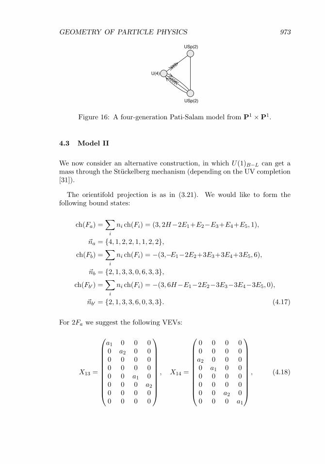
For 2Fa we suggest the following VEVs:
X13 =
⎛⎜⎜⎜⎜⎜⎜⎜⎜⎜⎜⎝
a1 0 0 00 a2 0 00 0 0 00 0 0 00 0 a1 00 0 0 a20 0 0 00 0 0 0
⎞⎟⎟⎟⎟⎟⎟⎟⎟⎟⎟⎠
, X14 =
⎛⎜⎜⎜⎜⎜⎜⎜⎜⎜⎜⎝
0 0 0 00 0 0 0a2 0 0 00 a1 0 00 0 0 00 0 0 00 0 a2 00 0 0 a1
⎞⎟⎟⎟⎟⎟⎟⎟⎟⎟⎟⎠
, (4.18)
974 MARTIJN WIJNHOLT
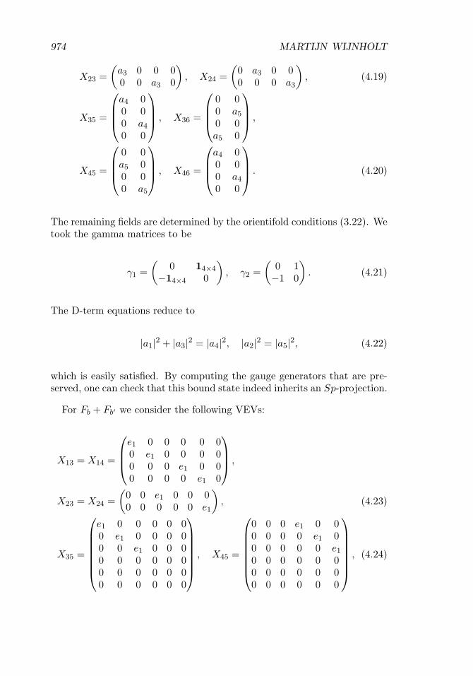
X23 =(
a3 0 0 00 0 a3 0
), X24 =
(0 a3 0 00 0 0 a3
), (4.19)
X35 =
⎛⎜⎜⎝
a4 00 00 a40 0
⎞⎟⎟⎠ , X36 =
⎛⎜⎜⎝
0 00 a50 0a5 0
⎞⎟⎟⎠ ,
X45 =
⎛⎜⎜⎝
0 0a5 00 00 a5
⎞⎟⎟⎠ , X46 =
⎛⎜⎜⎝
a4 00 00 a40 0
⎞⎟⎟⎠ . (4.20)
The remaining fields are determined by the orientifold conditions (3.22). Wetook the gamma matrices to be
γ1 =(
0 14×4−14×4 0
), γ2 =
(0 1
−1 0
). (4.21)
The D-term equations reduce to
|a1|2 + |a3|2 = |a4|2, |a2|2 = |a5|2, (4.22)
which is easily satisfied. By computing the gauge generators that are pre-served, one can check that this bound state indeed inherits an Sp-projection.
For Fb + Fb′ we consider the following VEVs:
X13 = X14 =
⎛⎜⎜⎝
e1 0 0 0 0 00 e1 0 0 0 00 0 0 e1 0 00 0 0 0 e1 0
⎞⎟⎟⎠ ,
X23 = X24 =(
0 0 e1 0 0 00 0 0 0 0 e1
), (4.23)
X35 =
⎛⎜⎜⎜⎜⎜⎜⎝
e1 0 0 0 0 00 e1 0 0 0 00 0 e1 0 0 00 0 0 0 0 00 0 0 0 0 00 0 0 0 0 0
⎞⎟⎟⎟⎟⎟⎟⎠
, X45 =
⎛⎜⎜⎜⎜⎜⎜⎝
0 0 0 e1 0 00 0 0 0 e1 00 0 0 0 0 e10 0 0 0 0 00 0 0 0 0 00 0 0 0 0 0
⎞⎟⎟⎟⎟⎟⎟⎠
, (4.24)

GEOMETRY OF PARTICLE PHYSICS 975
X36 =
⎛⎜⎜⎜⎜⎜⎜⎝
0 0 0 0 0 00 0 0 0 0 00 0 0 0 0 00 0 0 0 0 e10 0 0 e1 0 00 0 0 0 e1 0
⎞⎟⎟⎟⎟⎟⎟⎠
, X46 =
⎛⎜⎜⎜⎜⎜⎜⎝
0 0 0 0 0 00 0 0 0 0 00 0 0 0 0 00 0 e1 0 0 0e1 0 0 0 0 00 e1 0 0 0 0
⎞⎟⎟⎟⎟⎟⎟⎠
, (4.25)
with the remaining VEVs determined by (3.22). Here we took the gammamatrices to be
γ1 =(
0 12×2−12×2 0
), γ2 =
(0 1
−1 0
). (4.26)
The D-terms are satisfied. Note that we have used the notation Fb + Fb′ toindicate that this representation has two unbroken U(1)’s. They get mappedinto each other under the orientifolding.
After orientifolding the quiver generated by {2Fa, 3F3, F4, Fb + Fb′ , F7,3F8} we get a quiver with the expected chiral matter content of the MSSM,with three generations, and Higgs fields. These are some of the most com-plicated bound states in this paper, and we have not been able to check thatall excess non-chiral matter can be lifted by an induced superpotential.
We can also argue that all the remaining U(1)’s couple to an independentStuckelberg field. This is not automatically true but can be checked inthis case. To see this, before Higgsing and orientifolding the Stuckelbergcouplings are of the form
∑nodes i
∫C(i) ∧ Tr(F(i)), (4.27)
where C(i), F(i) are the Stuckelberg 2-form field and gauge field for the ithnode. After Higgsing we get
∑i,j
nji
∫C(i) ∧ Tr(F(j)), (4.28)
where nji is the number of original fractional branes of type i contained in
the bound state j, j ∈ {a, 3, 4, b, b′, 7, 8}, and F(j) is the corresponding gaugefield. Now it is easy to check that for our MSSM configuration the rank ofnj
i is maximal, so that all the U(1)’s couple to an independent Stuckelbergfield. We conclude that the U(1)B−L gauge boson can be lifted through theStuckelberg mechanism.
976 MARTIJN WIJNHOLT
5 Dynamical SUSY breaking
Since Del Pezzo quivers are chiral, one may expect to find examples of localmodels with dynamical supersymmetry breaking. However, it was typicallyfound in examples that if SUSY breaking occurred there was some runawaymode which invalidated the model [32–36]. Some effort has gone in to findinga way to stabilize such runaway modes [37–39].
We have seen that orientifolding eliminates Kahler moduli, so one mayrevisit this issue by looking for simple models where the runaway mode isprojected out. In fact, the new techniques allow us to engineer many familiarmodels which are known to break SUSY dynamically. Examples include:
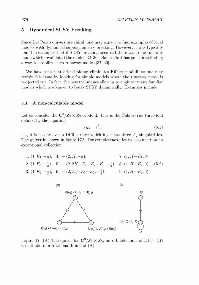
5.1 A non-calculable model
Let us consider the C3/Z3 × Z3 orbifold. This is the Calabi–Yau three-folddefined by the equation
xyz = t3, (5.1)
i.e., it is a cone over a DP6 surface which itself has three A2 singularities.The quiver in shown in figure 17A. For completeness, let us also mention anexceptional collection:
1. (1, E4,−12), 4. − (2, H, −1
2), 7. (1, H−E1, 0),
2. (1, E5,−12), 5. − (2, 2H−E1−E2−E3,−1
2), 8. (1, H−E2, 0),
3. (1, E6,−12), 6. − (2, E4+E5+E6,−3
2), 9. (1, H−E3, 0),
(5.2)
Figure 17: (A) The quiver for C3/Z3 × Z3, an orbifold limit of DP6. (B)Orientifold of a fractional brane of (A).

GEOMETRY OF PARTICLE PHYSICS 977
Figure 18: The dimer for the C3/Z3 × Z3 orbifold. The orientifold acts bya 180◦ rotation centered at the cross.
Now we are interested in the canonical orientifold action on the nodes,which exchanges oppositely twisted sectors:11
1 → 1∗, 2 → 3∗, 4 → 9∗, 5 → 8∗, 6 → 7∗. (5.3)
This is a symmetry of the dimer diagram, as indicated in figure 18. Letus take the fractional brane which only uses nodes {1, 5, 8}, as shown infigure 17. This is a model with two gauge groups, U(5) and O(1) = {±1}.The U(1) ⊂ U(5) gets a mass through the Stuckelberg mechanism, so weare left only with the SU(5), with matter in the 10 + 5. Since there areno gauge invariant baryonic operators we can write down, integrating outthe massive U(1) leads to a D-term potential for the dynamical FI-term(a normalizable closed string mode), stabilizing it. Thus what we are leftover with is precisely the model considered by [40]. This model has noclassical flat directions and a non-anomalous R-symmetry that was arguedto be broken, and therefore supersymmetry is broken dynamically.
An important property of this gauge theory is that it has very few param-eters, so there is little room for a runaway of the parameters after couplingto 4D gravity. Moreover, coming from such a simple singularity, the modelshould not be so hard to embed in a compact CY. For instance, we can easilyembed the singularity in the quintic, by taking an equation of the form
0 = s2(xyz − t3) + x5 + x4s + · · · (5.4)
11This is the orientifold action we intended to use in version 1 of this paper, by anal-ogy with the C3/Z3 orientifold of Section 3.2, but the picture in v1 showed a differentorientifold action. It is not hard to see that with the latter action, with an antisymmetricprojection of the rank 2 tensors and an orthogonal projection on fixed nodes, the orbifoldsuperpotential would not be invariant, though we are of course allowed to deform thesuperpotential.

978 MARTIJN WIJNHOLT
or we could try to use T 6/Z3 × Z3. To complete the analysis we would needto check that the orientifold can be extended globally and tadpoles can becancelled.
It would be nice to see the supersymmetry breaking from a dual gravityperspective. There is presumably an enhancon type of effect at work, similarto [41,42].
5.2 The 3-2 model
Our next model is a little harder to produce, so we start by drawing thequiver diagram in figure 19A, and its oriented cover in figure 19B. This isknown as the 3-2 model [43]. The stringy version has an additional anoma-lous U(1), which does not affect the low-energy dynamics as in the previousexample. There are various large N generalizations which appear to haveno classical flat directions and a spontaneously broken R-symmetry, and soshould also break supersymmetry.
The covering quiver has a certain similarity with DP5. So we take theDP5 quiver with the projections (3.19) and a = b = −1, with Sp-projectionson nodes 1 and 5, and SO-projections on nodes 2 and 6. We take
γ2 = 13×3, γ6 = 15×5 (5.5)
and consider a bound state Fa with charge vector
ch(Fa) =∑
i
ni ch(Fi), �n = {0, 3, 2, 3, 0, 5, 3, 2}. (5.6)
Figure 19: (A) The 3-2 model, with an extra massive U(1). (B) Orientedcover of the quiver in (A).
GEOMETRY OF PARTICLE PHYSICS 979
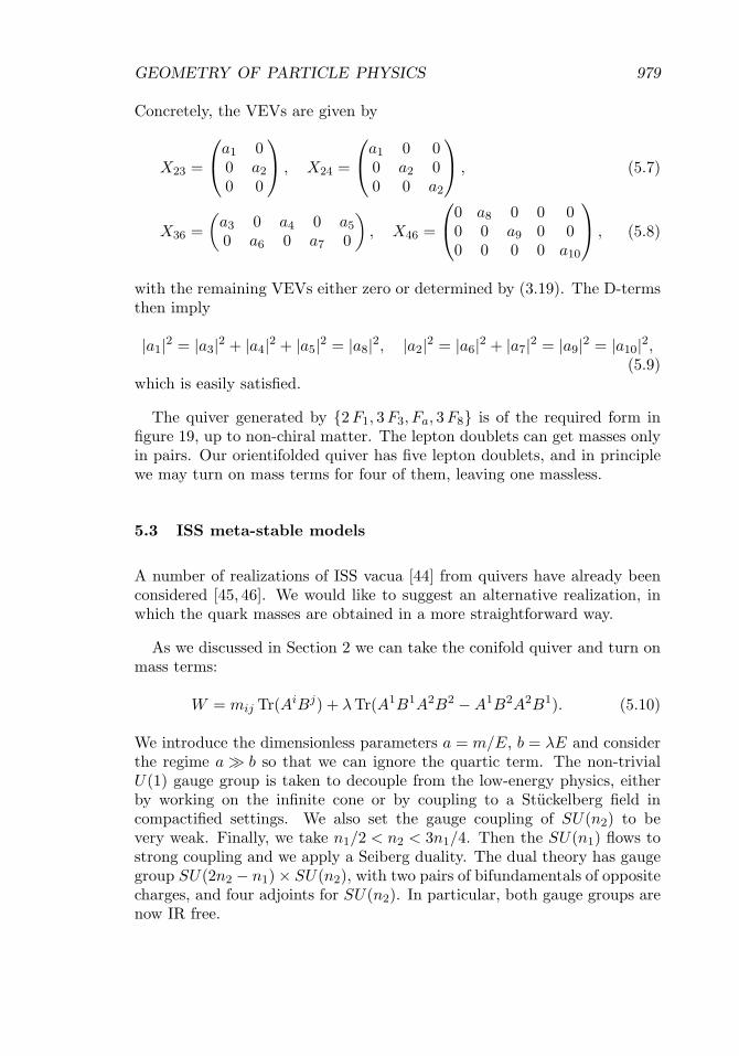
Concretely, the VEVs are given by
X23 =
⎛⎝a1 0
0 a20 0
⎞⎠ , X24 =
⎛⎝a1 0 0
0 a2 00 0 a2
⎞⎠ , (5.7)
X36 =(
a3 0 a4 0 a50 a6 0 a7 0
), X46 =
⎛⎝0 a8 0 0 0
0 0 a9 0 00 0 0 0 a10
⎞⎠ , (5.8)
with the remaining VEVs either zero or determined by (3.19). The D-termsthen imply
|a1|2 = |a3|2 + |a4|2 + |a5|2 = |a8|2, |a2|2 = |a6|2 + |a7|2 = |a9|2 = |a10|2,(5.9)
which is easily satisfied.
The quiver generated by {2 F1, 3 F3, Fa, 3 F8} is of the required form infigure 19, up to non-chiral matter. The lepton doublets can get masses onlyin pairs. Our orientifolded quiver has five lepton doublets, and in principlewe may turn on mass terms for four of them, leaving one massless.
5.3 ISS meta-stable models
A number of realizations of ISS vacua [44] from quivers have already beenconsidered [45, 46]. We would like to suggest an alternative realization, inwhich the quark masses are obtained in a more straightforward way.
As we discussed in Section 2 we can take the conifold quiver and turn onmass terms:
W = mij Tr(AiBj) + λ Tr(A1B1A2B2 − A1B2A2B1). (5.10)
We introduce the dimensionless parameters a = m/E, b = λE and considerthe regime a � b so that we can ignore the quartic term. The non-trivialU(1) gauge group is taken to decouple from the low-energy physics, eitherby working on the infinite cone or by coupling to a Stuckelberg field incompactified settings. We also set the gauge coupling of SU(n2) to bevery weak. Finally, we take n1/2 < n2 < 3n1/4. Then the SU(n1) flows tostrong coupling and we apply a Seiberg duality. The dual theory has gaugegroup SU(2n2 − n1) × SU(n2), with two pairs of bifundamentals of oppositecharges, and four adjoints for SU(n2). In particular, both gauge groups arenow IR free.
980 MARTIJN WIJNHOLT
Thus now we are in the situation of ISS, except that we have gauged aslightly different subgroup of the global symmetry group when the gaugecoupling for SU(n2) is finite. In this theory SUSY is broken by the rankcondition, and there are meta-stable vacua for zero adjoint VEVs with pseu-domoduli lifted by a one-loop potential. Actually if we would have kept thequartic terms of the conifold quiver then we get mass terms for the mesonsand we can solve the F-terms, but because we took a � b these SUSY vacuaare very far out in meson field space and do not affect the analysis near theorigin.
In the meta-stable vacua, the gauge group SU(2n2 − n1) × SU(n2) is bro-ken to SU(2n2 − n1) × SU(n1 − n2). If the SU(n2) gauge coupling is smallenough, then both the gauge couplings of the remaining SU(2n2 − n1) ×SU(n1 − n2) are also very small. There are also some massless Goldstonebosons left from the broken global symmetries, and some light fermions. TheGoldstone bosons parametrize a compact coset G/H and are not chargedunder the remaining gauge groups. Thus the remaining gauge groups mayeventually become strong in the deep IR and generate some vacuum energy.But since the strong coupling scale is arbitrarily small, this means theremust still be long-lived meta-stable vacua close to those found by ISS.
6 Topological criteria for unification
From the bottom-up perspective, there is no a priori relation between theMSSM couplings. For instance the differences between the (inverse squared)gauge couplings depend on complexified Kahler moduli. If such moduliextend to the UV completion, we will have to find a suitable potential tostabilize them, and it seems there is no natural reason to expect any relationbetween them.
On the other hand, we clearly do not live at a random point on theparameter space. There are many relations among the couplings that webelieve to be a reflection of new physics. So one may ask if these relationshave a special significance in our set-up.
Recently, it has been argued that moduli corresponding to non-normalizable closed string modes may be trivializable, in the sense thatthey appear to exist locally but may not be extended to the UV comple-tion [31]. (A similar scheme for the 6-volume was proposed in [47]). Thisis really a rephrasing of the obvious fact that the most interesting UV com-pletions are those which are as rigid as possible, consistent with observedlow-energy physics, because they give a topological explanation of the tree
GEOMETRY OF PARTICLE PHYSICS 981
level relations between certain couplings, as opposed to a dynamical one dueto moduli stabilization. It also reduces the number of global tadpoles to becancelled.
Let us review some aspects of this trivialization for Kahler moduli. Sup-pose that two fractional branes wrap vanishing cycles a and b, giving riseto a gauge group U(na) × U(nb), embedded in some orientifold compactifi-cation. Locally the homology class a − b has an even lift and an odd lift,where even and odd refer to the eigenvalue of the homology classes underthe orientifold action. Let us further assume that a − b is the class of a2-cycle that does not intersect a vanishing 4-cycle. Then if the odd lift istrivializable, we have the tree level relation
4π
g2a
− iϑa
2π=
4π
g2b
− iϑb
2π(6.1)
and if the even lift is trivializable we have
ζa + ica = ζb + icb, (6.2)
where ζ couples as an FI-term and c is its axion partner. A certain linearrelation between the axions is needed to keep hypercharge massless.
Now suppose for ease of discussion that both lifts are trivializable, so thata and b are the same cycle homologically. We can model this by consideringa single fractional brane with an adjoint scalar field whose superpotentialhas two critical points. Thus, morally the vacuum where the two branes sitapart is a Higgsed vacuum of a unified theory with gauge group U(na + nb),in particular the tree level gauge couplings of U(na) and U(nb) are relatedas above. Integrating out the massive adjoint we generate certain higherorder superpotential couplings suppressed by the mass of the adjoint field,which should correspond to the subleading complex structure deformationsdiscussed in [31].
This also explains the origin of the monopoles discovered in [48]: they areD-branes stretched between the gauge branes, i.e., they are the monopolesin the Higgsed phase expected by a Pati–Salam like unification in the modelof [2]. The unified model is actually one of the standard quivers for P2, withgauge group U(4) × U(2) × U(2) and (3, 6, 3) arrows between them.
Let us discuss how these ideas can be applied to the MSSM models thatwe have constructed from Del Pezzo 5. For the quivers and labelling ofthe nodes we refer to the figures in Section 1.2. The moduli controlling thedifference between the gauge couplings of U(3) node and the U(1)L node are
982 MARTIJN WIJNHOLT
trivialisable, so we can give a topological explanation of the relation g−23 =
g−21 . We can achieve this by making sure that E4 − E5 or H − E1 − E2 − E3
is globally trivial. If we assume that both are globally trivial, then we canmorally think of the U(3) and U(1) as being unified in the Pati–Salam groupU(4) (i.e., we have baryon–lepton unification). In fact, with only a smallchange in interpretation this situation was already proposed in [49,50].
The further relations12 g2 = g0 = g3 look quite natural because they cor-respond to the branes having equal tension, and they also give precisely thestandard tree level relations from SU(5) unification for the strong, weakand hypercharge couplings [49]. But they cannot be imposed by topologi-cal means, because the intersection numbers of the corresponding cycles aredifferent. However we can do the following. The tree level gauge couplingg3 corresponds to
2g23
=N
gs�2s
∫α
B2, α = E4 − E3, (6.3)
which is a non-normalizable mode in the local geometry. Here N is a numer-ical factor which depends on the periodicity of B2. Similarly13
1g22
+1g20
=N
gs�2s
∫β
B2 (6.4)
is a non-normalizable mode, where β is some degree zero linear combinationof the 2-cycles which depends on how we exactly constructed the boundstates.14 So any linear combination of these quantities is the integral ofthe B-field over some degree zero homology class, and therefore potentiallytrivializable. Together with g3 = g1 this then leads to a tree level relationbetween the observed gauge couplings
1g2Y
+1
g2W
=[2n1
n2+
23
]1g2S
, (6.5)
where we have assumed that n1α − n2β is trivialized. This is compatiblewith the relations from SU(5) unification, g−2
S = g−2W = 3
5g−2Y if we take β =
α in homology.
12Due to different normalizations of abelian and non-abelian charges, for model II equaltension of the branes corresponds to g2 =
√2g0 = g3.
13For model II this would read 12g−2
0 + g−22 = Ng−1
s �−2s
∫β
B2.14Actually this relation is not quite true with the bound states we constructed earlier.
However, it would have been true had we avoided the fractional brane F6 in our boundstates, at the cost of making the bound states slightly more complicated, and changingthe orientifold projection in the case of model II. Alternatively we could replace nodes 1and 3 by bound states which include F6.
GEOMETRY OF PARTICLE PHYSICS 983
Since∫α B2 −
∫β B2 =
∫γ H3, where ∂γ = α − β, one might wonder if these
tree level relations are not affected if we turn on background fluxes.15 Thisseems unlikely for the following reason. As long as no background fields areturned on we should expand the B-field in harmonic forms and the above cri-terion is sufficient to guarantee that the gauge couplings are related. Whenwe turn on general closed string deformations it is not necessarily true thatthe B-field must be expanded in harmonic forms; however, it is unlikely thatwe gain additional zero modes and so the relation between the couplings,which is due to a lack of zero modes, should not be affected.
7 Final thoughts
It should be clear by now that the set of quiver gauge theories that can beobtained from branes at singularities is rather large. It is our impressionthat virtually any quiver can be constructed locally, and we believe this isreally the main message of this paper. It will probably not be possible tocouple every such model to 4D gravity, but given a local model it will bevery hard to argue that it cannot be consistently coupled to gravity.
One would like to understand if the local D-brane scenario has somethingto add to discussions of beyond the SM physics. On the one hand it seemspremature. After many years of work, the field theory community has notbeen able to come up with a single model that adresses all concerns. Stringphenomenology is going to have to address the same issues, and barringa miraculous discovery of the correct UV completion it would be naive toexpect that doing string phenomenology would magically improve on thissituation. On the other hand, string phenomenology has traditionally beenmore a source of new ideas and intuition than a source of accurate models.
One way to proceed is to try and isolate desirable features and translatethem into geometrical or even topological terms. We have already discusseda topological explanation for tree level relations between gauge couplings.Other important issues are flavour problems. For instance we would liketo explain hierarchies among the Yukawa couplings, and we would like toexplain why new physics does not generate large flavour-changing neutralcurrents (FCNCs). Can we translate these criteria into geometric terms,and perhaps guarantee them through topological mechanisms similar toSection 6? Such rigidity requirements may eliminate the majority of UVcompletions in the string landscape.
15We would like to thank Angel Uranga for pointing out this possibility.
984 MARTIJN WIJNHOLT
Another important criterion will be stability. The apparent long-livednature of our universe suggests that we are in a vacuum which does not havetoo many vacua in its neighbourhood with a large cumulative probabilityto decay away to.16 This makes stability a very acute issue with possiblepredictive power, and we might expect string theory to have something tosay about this.
The bottom-up perspective also allows us to take a step back and seeif top-down approaches could benefit from new ingredients. It seems thatnon-commutative internal geometries play an important role. Thus perhapswe should be paying more attention to backgrounds of the type recentlyconstructed in [52].
7.1 On soft SUSY breaking
In this paper we have repeatedly used the technique of deforming the gaugetheory to get rid off undesirable particles. By the same logic we can proceedto turn on masses for all the superpartners of the Standard Model fieldsand recover the non-SUSY Standard Model itself. This must be possible,but it is not terribly helpful. Although the dictionary between the localgeometry and the superpotential deformations used in this paper are fairlywell understood and can in principle be solved exactly, unfortunately thedictionary for SUSY breaking deformations is more complicated. It requiresunderstanding Kaehler deformations which can probably only be addressednumerically, and it requires further generalizing the notion of geometry inways that are probably not yet quite understood. Even for simpler theorieslike N = 4 Yang–Mills, little is known about the stringy description of non-supersymmetric deformations. Progress can perhaps be made if one canidentify special points on the parameter space where the stringy descriptionsimplifies.
7.2 Composite Higgses?
A rather curious feature of the MSSM quiver is that, if we started withoutHiggs fields, we can automatically generate them through Seiberg dualityon U(3)c or U(1)L. For the U(3) node, Seiberg duality has been consideredby Matt Strassler [53], who was looking for a possible embedding into a
16In fact, it has recently been argued [51] in a “bottom-up” approach, quite independentof string theory, that the landscape of the SM plus quantum gravity may contain vacuaclose to ours which correspond to compactification to lower dimensions.

GEOMETRY OF PARTICLE PHYSICS 985
duality cascade, and also in [54]. A problem in that case is that one needsto add extra massive matter in order to make the SU(3) coupling growstrong towards the UV.
In the MSSM quivers we have an alternative: we may consider a “Seibergduality” on the U(1)L node (node 1 in the figures of Section 1.2). The dualgroup is U(5) or larger and we are automatically have Nf = Nc + 1, so wedo not have to add additional matter to get a consistent picture. Since theU(1) ⊂ U(5) and the SU(5) ⊂ U(5) run independently, this may even beconsistent with unification, but we have not done the calculation. As theSU(5) flows to strong coupling towards the IR, the electric “quarks” bindinto mesons which have the same quantum numbers as the Higgses, althoughthe large number we get is not so desirable. Their number may be reducedif we also have Higgs fields with appropriate couplings in the electric theory.Thus perhaps if the supersymmetry breaking scale is significantly lower thanthe scale at which we would have to apply a Seiberg duality, the Higgsesmay be interpreted as composite fields, and this might be the seed of anexplanation why one pair ends up being relatively light.
7.3 The QCD string as a fundamental string
One may wonder if our set-up gives any insight into the stringy descriptionof QCD. Let us turn on Higgs VEVs so that the quarks obtain small masses.Then in the IR we may focus on the U(3) node which gives us pure SU(3)SUSY QCD. Now note that the U(3) brane (together with its orientifoldimage) has wrapping numbers (0, E4 − E3, 0). So as the theory flows tostrong coupling what most likely happens is that the Del Pezzo undergoes aconifold transition, where a small 2-sphere in the class E4 − E3 gets replacedby a 3-sphere. After the transition, the U(3) brane has been replaced by flux,and thus the open strings ending on this brane are confined. The glueballcondensate is described by a closed string mode, as envisaged in [55].
Thus in our picture the graviton and the QCD string can be described asdifferent modes of the same fundamental string, the IIB string. As we discussmomentarily though, in some situations the graviton is better described asa mode of the heterotic string.
7.4 Weakly coupled Planck brane?
As we reach the Planck brane, we will start to see other ingredientsof the compactification: D7’s and orientifold planes (which split up
986 MARTIJN WIJNHOLT
non-perturbatively as mutually non-local D7-branes). Generically the IIbstring coupling cannot be kept small, and the IIB description may be lessthan useful. However there may exist a large class of UV completions wherethe Planck brane has a dual description in terms of weakly coupled heteroticstrings.
The fractional brane configuration only has net D3 and D5 charge, soit should get mapped to a small (possibly constrained) instanton in theheterotic string. As the instanton shrinks to zero, it generates a throat andthus potentially a large hierarchy. This is the heterotic manifestation ofthe decoupling limit. The heterotic dilaton grows down the throat, so theMSSM is non-perturbative from this point of view.
In the perturbative heterotic description we cannot see the enhancedgauge symmetry due to fractionation, since the individual fractional braneshave D7-brane charges. Thus the fractional branes should have merged intoa single NS5-brane when the heterotic coupling is small. This by itself doesnot mean that the gauge couplings should unify at the cross-over scale,although it seems like a natural boundary condition.
Acknowledgments
It is a pleasure to thank Sebastian Franco, Sam Pinansky and Herman Ver-linde for discussions. I would also like to thank CERN and the Max PlanckInstitute in Munich for hospitality and the opportunity to present some ofthese results.
References
[1] G. Aldazabal, L. E. Ibanez, F. Quevedo and A. M. Uranga, D-branesat singularities: A bottom-up approach to the string embedding of thestandard model, JHEP 0008 (2000) 002 [arXiv:hep-th/0005067].
[2] H. Verlinde and M. Wijnholt, Building the standard model on a D3-brane; arXiv:hep-th/0508089.
[3] D. Berenstein, V. Jejjala and R. G. Leigh, The standard model on aD-brane, Phys. Rev. Lett. 88 (2002), 071602 [arXiv:hep-ph/0105042].
[4] J. Gray, Y. H. He, V. Jejjala and B. D. Nelson, The geometry of particlephysics, Phys. Lett. B 638 (2006), 253 [arXiv:hep-th/0511062].J. Gray, Y. H. He, V. Jejjala and B. D. Nelson, Exploring the vac-uum geometry of N= 1 gauge theories, Nucl. Phys. B 750 (2006), 1[arXiv:hep-th/0604208].
GEOMETRY OF PARTICLE PHYSICS 987
[5] L. E. Ibanez, F. Marchesano and R. Rabadan, Getting just thestandard model at intersecting branes, JHEP 0111 (2001), 002[arXiv:hep-th/0105155].
[6] M. Cvetic, G. Shiu and A. M. Uranga, Chiral four-dimensional N= 1supersymmetric type IIA orientifolds from intersecting D6-branes, Nucl.Phys. B 615 (2001), 3 [arXiv:hep-th/0107166].C. Kokorelis, New standard model vacua from intersecting branes,JHEP 0209 (2002), 029 [arXiv:hep-th/0205147].F. Gmeiner, R. Blumenhagen, G. Honecker, D. Lust and T. Weigand,One in a billion: MSSM-like D-brane statistics, JHEP 0601 (2006),004 [arXiv:hep-th/0510170].
[7] T. P. T. Dijkstra, L. R. Huiszoon and A. N. Schellekens, Supersymmet-ric standard model spectra from RCFT orientifolds, Nucl. Phys. B 710(2005), 3 [arXiv:hep-th/0411129].
[8] R. Blumenhagen, M. Cvetic, P. Langacker and G. Shiu, Toward realisticintersecting D-brane models, Ann. Rev. Nucl. Part. Sci. 55 (2005), 71[arXiv:hep-th/0502005].
[9] D. Berenstein and S. Pinansky, The minimal quiver standard model ;arXiv:hep-th/0610104.
[10] S. Kachru, J. Pearson and H. L. Verlinde, Brane/flux annihilationand the string dual of a non-supersymmetric field theory, JHEP 0206(2002), 021 [arXiv:hep-th/0112197].
[11] M. Kontsevich, Homological algebra of mirror symmetry,[arxiv:alg-geom/9411018].
[12] M. R. Douglas and G. W. Moore, D-branes, Quivers, and ALE Instan-tons, arXiv:hep-th/9603167.
[13] D. R. Morrison and M. R. Plesser, Non-spherical horizons. I, Adv.Theor. Math. Phys. 3 (1999), 1 [arXiv:hep-th/9810201].
[14] C. E. Beasley, Superconformal theories from branes at singularities,Duke University senior honors thesis, 1999.
[15] C. Beasley, B. R. Greene, C. I. Lazaroiu and M. R. Plesser, D3-braneson partial resolutions of abelian quotient singularities of Calabi-Yauthreefolds, Nucl. Phys. B 566 (2000), 599 [arXiv:hep-th/9907186].
[16] B. Feng, A. Hanany and Y. H. He, D-brane gauge theories fromtoric singularities and toric duality, Nucl. Phys. B 595 (2001), 165[arXiv:hep-th/0003085].
[17] M. R. Douglas, B. Fiol and C. Romelsberger, The spectrum ofBPS branes on a noncompact Calabi-Yau, JHEP 0509 (2005), 057[arXiv:hep-th/0003263].

988 MARTIJN WIJNHOLT
[18] F. Cachazo, B. Fiol, K. A. Intriligator, S. Katz and C. Vafa,A geometric unification of dualities, Nucl. Phys. B 628 (2002), 3[arXiv:hep-th/0110028].
[19] M. Wijnholt, Large volume perspective on branes at singularities, Adv.Theor. Math. Phys. 7 (2004), 1117 [arXiv:hep-th/0212021].
[20] M. Wijnholt, Parameter space of quiver gauge theories;arXiv:hep-th/0512122.
[21] A. Bergman and N. J. Proudfoot, Moduli spaces for D-branes at the tipof a cone, JHEP 0603 (2006), 073 [arXiv:hep-th/0510158].
[22] P. S. Aspinwall, D-branes, II-stability and Theta-stability ;arXiv:hep-th/0407123.
[23] T. Bridgeland, Stability conditions on a non-compact Calabi-Yau threefold, Commun. Math. Phys. 266 (2006), 715 [arXiv:math.ag/0509048].
[24] C. P. Herzog and J. Walcher, Dibaryons from exceptional collections,JHEP 0309 (2003), 060 [arXiv:hep-th/0306298].
[25] C. P. Herzog and R. L. Karp, On the geometry of quivergauge theories: stacking exceptional collections, arXiv:hep-th/0605177.
[26] K. Hori and J. Walcher, D-brane categories for orientifolds: TheLandau–Ginzburg case, arXiv:hep-th/0606179.
[27] D. E. Diaconescu, A. Garcia-Raboso, R. L. Karp and K. Sinha,D-brane superpotentials in Calabi-Yau orientifolds (projection),arXiv:hep-th/0606180.
[28] J. D. Lykken, E. Poppitz and S. P. Trivedi, Branes with GUTsand supersymmetry breaking, Nucl. Phys. B 543 (1999), 105[arXiv:hep-th/9806080].
[29] R. Blumenhagen, V. Braun, B. Kors and D. Lust, Orientifolds ofK3 and Calabi-Yau manifolds with intersecting D-branes, JHEP 0207(2002), 026 [arXiv:hep-th/0206038].
[30] S. Franco, A. Hanany, K. D. Kennaway, D. Vegh and B. Wecht,Brane dimers and quiver gauge theories, JHEP 0601 (2006), 096[arXiv:hep-th/0504110].
[31] M. Buican, D. Malyshev, D. R. Morrison, M. Wijnholt and H. Ver-linde, D-branes at singularities, compactification, and hypercharge,arXiv:hep-th/0610007.
[32] D. Berenstein, C. P. Herzog, P. Ouyang and S. Pinansky, Supersym-metry breaking from a Calabi-Yau singularity, JHEP 0509 (2005), 084[arXiv:hep-th/0505029].
GEOMETRY OF PARTICLE PHYSICS 989
[33] S. Franco, A. Hanany, F. Saad and A. M. Uranga, Fractional branesand dynamical supersymmetry breaking, JHEP 0601 (2006), 011[arXiv:hep-th/0505040].
[34] M. Bertolini, F. Bigazzi and A. L. Cotrone, Supersymmetry breakingat the end of a cascade of Seiberg dualities, Phys. Rev. D 72 (2005),061902 [arXiv:hep-th/0505055].
[35] K. Intriligator and N. Seiberg, The runaway quiver, JHEP 0602 (2006),031 [arXiv:hep-th/0512347].
[36] A. Brini and D. Forcella, Comments on the non-conformal gaugetheories dual to Y(p,q) manifolds, JHEP 0606 (2006), 050[arXiv:hep-th/0603245].
[37] S. Franco and A. M. Uranga, Dynamical SUSY breaking at meta-stableminima from D-branes at obstructed geometries, JHEP 0606 (2006),031 [arXiv:hep-th/0604136].
[38] B. Florea, S. Kachru, J. McGreevy and N. Saulina, Stringy instantonsand quiver gauge theories, arXiv:hep-th/0610003.
[39] D. E. Diaconescu, R. Donagi and B. Florea, Metastable quivers in stringcompactifications, arXiv:hep-th/0701104.
[40] I. Affleck, M. Dine and N. Seiberg, Dynamical supersymmetry breakingin chiral theories, Phys. Lett. B 137 (1984), 187.
[41] C. V. Johnson, A. W. Peet and J. Polchinski, Gauge theory and theexcision of repulson singularities, Phys. Rev. D 61 (2000), 086001[arXiv:hep-th/9911161].
[42] M. Wijnholt and S. Zhukov, Inside an enhancon: monopolesand dual Yang–Mills theory, Nucl. Phys. B 639 (2002), 343[arXiv:hep-th/0110109].
[43] I. Affleck, M. Dine and N. Seiberg, Calculable nonperturbative super-symmetry breaking, Phys. Rev. Lett. 52 (1984), 1677.
[44] K. Intriligator, N. Seiberg and D. Shih, Dynamical SUSY breaking inmeta-stable vacua, JHEP 0604 (2006), 021 [arXiv:hep-th/0602239].
[45] H. Ooguri and Y. Ookouchi, Landscape of supersymmetry breakingvacua in geometrically realized gauge theories, Nucl. Phys. B 755(2006), 239 [arXiv:hep-th/0606061].
[46] R. Argurio, M. Bertolini, S. Franco and S. Kachru, Gauge/gravity dual-ity and meta-stable dynamical supersymmetry breaking, JHEP 0701(2007), 083 [arXiv:hep-th/0610212].
[47] K. Becker, M. Becker, C. Vafa and J. Walcher, Moduli stabilization innon-geometric backgrounds; arXiv:hep-th/0611001.
990 MARTIJN WIJNHOLT
[48] H. Verlinde, On metastable branes and a new type of magnetic mono-pole; arXiv:hep-th/0611069.
[49] R. Blumenhagen, D. Lust and S. Stieberger, Gauge unification insupersymmetric intersecting brane worlds, JHEP 0307 (2003), 036[arXiv:hep-th/0305146].
[50] I. Antoniadis, E. Kiritsis and T. N. Tomaras, A D-brane alternative tounification, Phys. Lett. B 486 (2000), 186 [arXiv:hep-ph/0004214].
[51] N. Arkani-Hamed, Talk at LMU University in Munich, January 22.[52] M. Grana, R. Minasian, M. Petrini and A. Tomasiello, A scan for new
N = 1 vacua on twisted tori ; arXiv:hep-th/0609124.[53] M. Strassler, Prepared for International workshop on perspectives of
strong coupling gauge theories (SCGT 96), Nagoya, Japan, 13–16 Nov.1996.
[54] N. Maekawa, Dualiy of a supersymmetric standard model, Prog. Theor.Phys. 95 (1996), 943 [arXiv:hep-ph/9509407].N. Maekawa and T. Takahashi, Duality of a supersymmetric modelwith the Pati–Salam group, Prog. Theor. Phys. 95 (1996), 1167[arXiv:hep-ph/9510426].
[55] I. R. Klebanov and M. J. Strassler, Supergravity and a confining gaugetheory: duality cascades and chisb-resolution of naked singularities,JHEP 0008 (2000), 052 [arXiv:hep-th/0007191].J. M. Maldacena and C. Nunez, Towards the large N limit ofpure N = 1 super Yang Mills, Phys. Rev. Lett. 86 (2001), 588[arXiv:hep-th/0008001].C. Vafa, Superstrings and topological strings at large N, J. Math. Phys.42 (2001), 2798 [arXiv:hep-th/0008142].