geometry of the space of phylogenetic treesfinmath.stanford.edu/~susan/papers/lap.pdf · geometry...

Geometry of the Space of Phylogenetic Trees

Louis J. Billera

Department of Mathematics, Malott Hall, Cornell University, Ithaca, NY 14853E-mail: [email protected]

and

Susan P. Holmes

INRA, Montpellier, France and Department of Statistics, Stanford University,Stanford, CA 94305

E-mail: [email protected]

and

Karen Vogtmann

Department of Mathematics, Malott Hall, Cornell University, Ithaca, NY 14853E-mail: [email protected]

We consider a continuous space which models the set of all phylogenetictrees having a fixed set of leaves. This space has a natural metric of nonpositive curvature, giving a way of measuring distance between phylogenetictrees and providing some procedures for averaging or combining several treeswhose leaves are identical. This geometry also shows which trees appear withina fixed distance of a given tree and enables construction of convex hulls of aset of trees.

This geometric model of tree space provides a setting in which questionsthat have been posed by biologists and statisticians over the last decade canbe approached in a systematic fashion. For example, it provides a justificationfor disregarding portions of a collection of trees that agree, thus simplifyingthe space in which comparisons are to be made.

Mathematics Subject Classification: 92D15, 92B10, 05C05, 62P10.

Keywords: Phylogenetic trees, semi-labeled trees, associahedron, CAT(0)space, consensus, bootstrap.

This work was supported, in part, by NSF grants DMS9800910, DMS9973891 andDMS 9971607.

1

2 BILLERA, HOLMES AND VOGTMANN

MOTIVATION

Trees have been used extensively in biology and other fields to graphicallyrepresent various types of hierarchical relationships, including evolutionaryrelationships between species, divergent patterns between subpopulationsand evolutionary relationships between genes. These trees are generallyrooted and semi-labeled, i.e., they descend from a single node called theroot, bifurcate at lower nodes and end at terminal nodes, called tips orleaves; the leaves are labeled by the names of the species, subpopulationsor genes being studied. In biological studies the latter are called operationaltaxonomic units (OTU’s).

Traditionally, trees were inferred form morphological similarities amongthe OTU’s. To build an evolutionary species tree, or phylogenetic tree, twospecies which shared the most characteristics were classified as ‘siblings’and assumed to share a common ancestor which is not the ancestor of anyother species. Such ‘siblings’ are said to be homologous, and it is this basichomology which has been of interest to biologists for a very long time.In Figure 1 we reproduce a tree from Haeckel (1866) which represents anattempt at depicting the relationships between all living organisms.

Over the last few decades, biologists have been building trees based onDNA sequences from certain parts of the genome. This has led to remark-able advances in the study of homology. Examples of the kinds of issues onwhich new light has been shed include the origin of diseases such as AIDS(Krushkal and Li (1998)) and the most deadly form of malaria (Escalanteand Ayala (1995)), and connections between tribal groups such as thoseraised by the African tribe whose oral tradition holds that the tribe is de-scended from Jewish priests (DNA analysis does indicate such a relation).

In spite of the successes of DNA analysis, a great deal of uncertaintyremains about precise relationships between the tips or leaves of the tree.Uncertainty about which branching order is the correct one is sometimesrepresented by filling out the tree as in Figure 2 to cover several possiblebinary trees and exclude others which biologists are sure are impossible.

SPACE OF PHYLOGENETIC TREES 3

Figure 1: Haeckel’s tree with 3 branches


Figure 2: Equus tree from (MacFadden, 1985)

For example Figure 2 from MacFadden (1985) implicitly rules out thepossibility of Sinohippus and Protohippus being homologous; however italso allows for indetermination of the branching order of Neohipparion,Pseudohipparion and Cormohipparion. In this paper we propose a geomet-ric model which parameterizes the set of trees with a fixed set of OTU’s;in this model, uncertainty can be represented by coloring in the portionsof the space corresponding to possible trees.


One reason for uncertainty about the true phylogenetic tree is that dif-ferent choices for DNA sequences (usually the choice of a single gene orcoding region) often point to different trees, each of which is called a ‘gene-tree’ (Doyle, 1992). Finding the best way of combining the informationcontained in numerous different gene-trees for the same set of species re-mains an open problem in contemporary biology. Several methods havebeen proposed to solve this combination problem. One proposal is to treatthe data from different genes as if they came from a single gene. For exam-ple, Brooks (1981) has suggested building all the different trees and thencoding the tree data into binary columns, combining them and finding thebest tree for the combined columns. Other proposed methods use somespecified set of combination rules such as majority rule, strict consensusor Bayesian combination. A difficulty with combining data from differentgenes into a single, larger data set arises from differences in the mutationrates in different genes. Another interesting effect is that in simulationstudies, where the true tree topology is known in advance, investigatorshave observed that a more accurate tree is obtained by subdividing thedata into many different sequences and then averaging by some methodthan by agglomerating all of the sequences and then building a single treewith the merged data. Perturbing the simulated data by bootstrap resam-pling and then averaging also produces a tree which is closer to the knownoriginal tree (Berry and Gascuel, 1996). This points to the importance ofunderstanding the rules used to average trees. None of the proposed con-sensus rules has previously been studied in a geometric context. Details oftheir comparison in the geometric context introduced in this paper will beexplained in Billera et al. (2001).

Uncertainty about the true phylogenetic tree arises also from problems ofstatistical stability. The classical tree-building algorithms attempt to find asingle tree consistent with the data. The question of how sure one is that thetree is correct is thus also a statistical one: the tree becomes an unknownparameter that the various procedures are trying to estimate. Would asmall change in the data resulting from a sequencing or an alignment errorresult in a change of choice of the resulting tree? This is currently studiedby using bootstrapping as a perturbation tool (Felsenstein, 1983), but infact this can be interpreted as a problem in the estimation process. Thisproblem has inspired certain authors (see Efron et al. (1996) and Zharkikhand Li (1995)) to imagine partitioning a space of trees into regions, eachlabeled by a different binary tree. When a data set is associated to a pointin this space, the question of the resulting tree’s stability can be translatedinto a question about how close the point is to the boundary betweendifferent regions. The question was raised in Zharkikh and Li (1995) as tohow many regions are within a certain range of a given point. The currentpaper attempts to give the intuitive arguments presented in the above cited


papers a rigorous geometric interpretation. In particular, since our spaceof trees has a metric, this allows a “Voronoi” decomposition into nearest-neighbor regions, that is, regions consisting of those trees closest to eachof a fixed finite set of trees (see Edelsbrunner (1987)).

One more reason for uncertainty about the true phylogenetic tree involvesthe tree-building process. The first problem encountered by taxonomistswho build phylogenetic trees using any of the several methods available isthe complexity of the underlying optimization problem. There are

(2n− 3)!! = (2n− 3)× (2n− 5)× . . . 3 =(2n− 2)!

2n−1(n− 1)!

rooted binary semi-labeled trees with n leaves (Schroder, 1870). The prob-lem of computing the best tree for a certain data set is NP complete fortwo of the most common methods, the maximum likelihood methods andthe parsimony methods (Foulds and Graham, 1982). As a consequence bi-ologists have to use approximate optimization algorithms that use randomstarting points and certain random moves between trees. The resultingtrees thus vary from run to run. The geometric model we introduce inthis paper allows one to compare these trees in a quantitative way. Suchcomparisons could be useful in contexts such as those discussed in Lin andGerstein (2000).

Biologists use a range of methods to construct trees from DNA sequences,each of which results in a tree with branch lengths. At one end of the spec-trum lie the parametric models, such as the maximum likelihood method.In this method, a probability is given for each possible base change in aDNA sequence, and the tree that maximizes the likelihood under this modelis the one chosen as the best estimate. Many biologists believe that as moredata becomes available the mutation rates will be known with better accu-racy and parametric models will be better justified. The geometric modelof tree space presented in this paper enables one to represent the maximumlikelihood tree as a point in a space of trees with branch lengths; it shouldthen be possible to define isocontour regions around the estimated tree tobuild the desired confidence regions.

In a parametric model, the data are approximated by points in a very low-dimensional manifold, thereby losing much of the information containedin the original data. The Jukes-Cantor model, for instance, uses an n-dimensional parameterization of the data corresponding to trees with nleaves. To get a rough idea of this, imagine asserting that the data pointslie on an ellipse and then choosing the two parameters of the ellipse so asto minimize the sum of the distances from the points to the ellipse. Theellipse is parameterized by two numbers, and represents the parametricmodel that biologists will try to fit the data to.


At the other end of the spectrum of tree-building methods lie the non-parametric models, such as the parsimony representation. A nonparametricapproach could simply interpolate between points; as the number of pointsincreases the number of descriptive parameters increases. A more sophisti-cated nonparametric approach would propose a smooth curve minimizingthe distance to the points. Thus nonparametric methods are also said tobe infinite dimensional. For instance, in the parsimony model, the tree isdefined to be the minimal Steiner tree compatible with the observed dis-tances between the OTU’s, the branch lengths then represent numbers ofmutation events.

In between these two extremes lie the distance-based methods, which aresemi-parametric models, in which the mutation model is parametric withvery few parameters (usually between one and four) and the tree buildingprocedure is non-parametric. See Holmes (1999) for a detailed comparisonof these three estimation paradigms.

Each method of producing trees from data results in trees with branchlengths, but these branch lengths have different meanings in different meth-ods. The choice of which procedure is used to produce trees will not affectthe geometric representation of the space of trees as we propose it here,but only the interpretation of points in the space.

A brief summary of the paper follows. In §1, we describe two preliminaryattempts to obtain a geometric setting for the study of trees, each closelyrelated to a convex polytope (the matching polytope and the associahe-dron). In §2 we give an explicit construction of the space of trees T n, andin §3 we give some of its basic combinatorial properties. While T n is nota manifold, the underlying combinatorial properties of trees help exposesome of its structure. In §4 we study the geometric properties of T n suchas curvature (the CAT(0) property), geodesics and centroids. We also dis-cuss ways to introduce probability measures on this space in order to finda geometric setting for the statistical study of tree data. We conclude in§5 with a discussion of some of the questions that arise when consideringsuch data.

1. TWO PRELIMINARY ATTEMPTS

In Diaconis and Holmes (1998), trees were coded as “matchings” on acomplete graph. These matchings allow trees to be identified with thevertices of a convex polytope, called the matching polytope (see Lovasz andPlummer (1985)). A shortcoming of this matching representation is thata small move on the matching polytope may have either a very small ora very large effect on the tree, as it interchanges two nodes which maybe either far from or close to the root. This asymmetry in the matching


representation is not present in the geometric representation presented inthis paper.

There is another convex polytope, called the associahedron (see Lee(1989) or Stasheff (1963)) whose vertices can be identified with the setof planar rooted binary trees with n leaves in a fixed order or, equivalently,with the set of triangulations of an (n + 1)-gon. The associahedron forn = 4 is a pentagon, and is illustrated in Figure 3; the triangulations areindicated by dotted lines and the corresponding binary trees are drawnwith solid lines. Two vertices of the associahedron are adjacent if thecorresponding triangulations differ by “rotating” a single interior edge e,i.e., removing e to form a quadrilateral in the interior of the (n + 1)-gonand then replacing e by the opposite diagonal of the quadrilateral. Thecorresponding trees are also said to be linked by rotation (see Figure 15).

0

1

2

3

4

0

1

2

3

4

0

1

2

3

4 0

1

2

3

4

0

1

2

3

4

Figure 3: Associahedron in the case n = 4

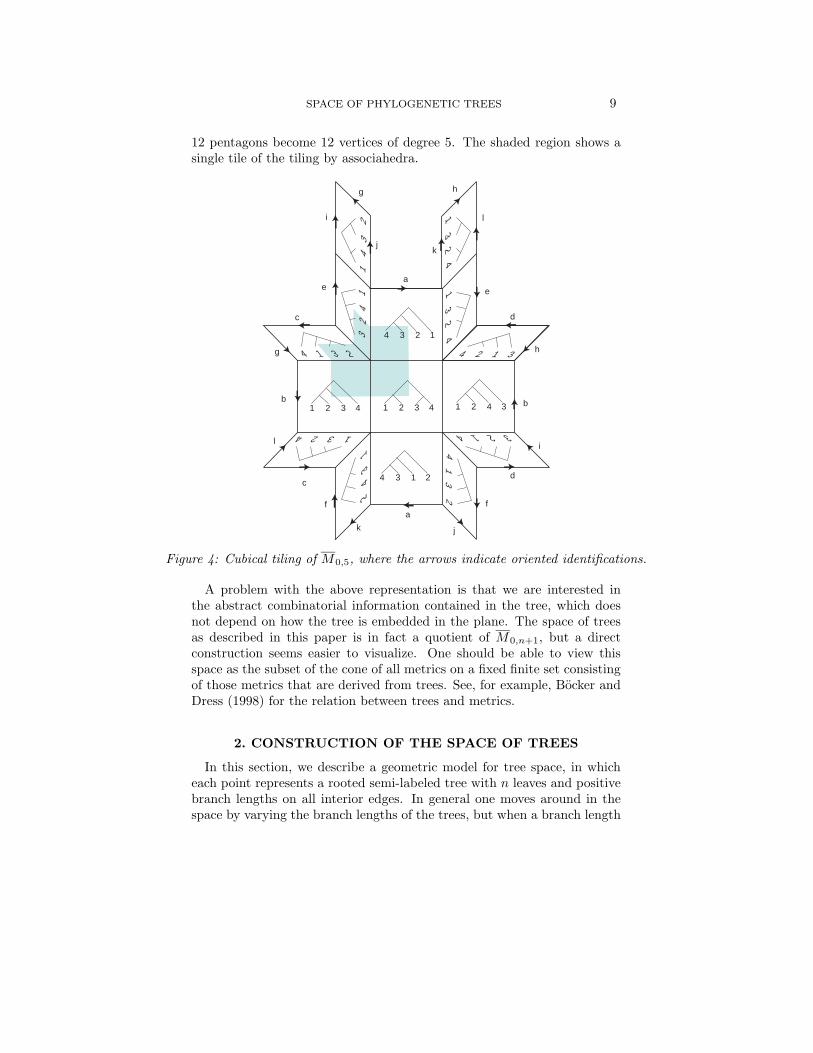
By “gluing” associahedra together, one can construct a space of planarlabeled trees with n leaves, where each associahedron corresponds to a dif-ferent ordering of the labels. This space has appeared in several differentcontexts (Davis et al., 1998; Devadoss, 1999; Kapranov, 1993), and is de-noted M0,n+1. The space M0,5 is tiled with 12 pentagons, correspondingto all possible permutations of the leaves up to complete reversal. Eachspace M0,n+1 has a dual tiling by (n − 3)-dimensional cubes. The dualtiling of M0,5, by squares, is illustrated in Figure 4; in the dual tiling, the


12 pentagons become 12 vertices of degree 5. The shaded region shows asingle tile of the tiling by associahedra.

1 2 3 4 1 2 4 31 2 3 4

4 3 2 1

g

a

a

bb

c

c

d

d

e e

f f

13

24

4 3 1 2

4 2 1 31

43

2

3214

4 1 3 2

2431

32

41 1

32

44

13

2

1324

g h

h

i

jk

l

k

li

j

Figure 4: Cubical tiling of M0,5, where the arrows indicate oriented identifications.

A problem with the above representation is that we are interested inthe abstract combinatorial information contained in the tree, which doesnot depend on how the tree is embedded in the plane. The space of treesas described in this paper is in fact a quotient of M0,n+1, but a directconstruction seems easier to visualize. One should be able to view thisspace as the subset of the cone of all metrics on a fixed finite set consistingof those metrics that are derived from trees. See, for example, Bocker andDress (1998) for the relation between trees and metrics.

2. CONSTRUCTION OF THE SPACE OF TREES

In this section, we describe a geometric model for tree space, in whicheach point represents a rooted semi-labeled tree with n leaves and positivebranch lengths on all interior edges. In general one moves around in thespace by varying the branch lengths of the trees, but when a branch length


reaches 0 some degeneration or uncertainty occurs which can be resolvedin one of several ways, each of which leads to a new tree.

We now proceed to formally define the space. The term n-tree will meana tree (i.e., a connected graph with no circuits), with a distinguished vertex,called the root, and n vertices of degree 1, called leaves, that are labeledfrom 1 to n. Although we are primarily interested in binary trees (i.e.,trees in which the root has degree 2 and all other vertices have degree 1or 3), in order to interpolate between these we will also need to considertrees whose vertices have larger degree. Perversely, mathematicians usuallyput the root at the top when drawing a picture of a tree, so that the tree“grows downward” from its root (see Figure 5).

root

leaves

interior edges

1 2 3 4 5

Figure 5: A semi-labeled binary tree

For technical reasons, it will often be convenient to “hang each tree upby its root,” i.e., to place an edge directly above the root of every tree, withthe corresponding leaf labeled with 0. Note that there are several ways ofdrawing a diagram of the same tree, depending on how it is embedded inthe plane. For example, the three pictures in Figure 6 represent the sametree.

1 42 3

0

1 32 4

0

2 14 3

0

Figure 6: Three pictures of the same tree

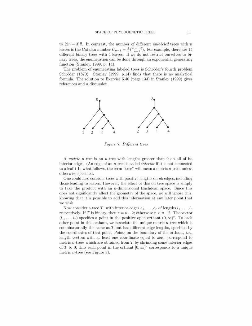
On the other hand, two trees that have exactly the same combinatorialstructure but whose leaves are labeled differently are considered different(see Figure 7). The number of different binary trees on n leaves is equal


to (2n − 3)!!. In contrast, the number of different unlabeled trees with n

leaves is the Catalan number Cn−1 = 1n

(2(n−1)n−1

). For example, there are 15

different binary trees with 4 leaves. If we do not restrict ourselves to bi-nary trees, the enumeration can be done through an exponential generatingfunction (Stanley, 1999, p. 14).

The problem of enumerating labeled trees is Schroder’s fourth problemSchroder (1870). Stanley (1999, p.14) finds that there is no analyticalformula. The solution to Exercise 5.40 (page 133) in Stanley (1999) givesreferences and a discussion.

1 42 3

0

2 43 1

0

Figure 7: Different trees

A metric n-tree is an n-tree with lengths greater than 0 on all of itsinterior edges. (An edge of an n-tree is called interior if it is not connectedto a leaf.) In what follows, the term “tree” will mean a metric n-tree, unlessotherwise specified.

One could also consider trees with positive lengths on all edges, includingthose leading to leaves. However, the effect of this on tree space is simplyto take the product with an n-dimensional Euclidean space. Since thisdoes not significantly affect the geometry of the space, we will ignore this,knowing that it is possible to add this information at any later point thatwe wish.

Now consider a tree T , with interior edges e1, . . . , er of lengths l1, . . . , lrrespectively. If T is binary, then r = n−2; otherwise r < n−2. The vector(l1, . . . , lr) specifies a point in the positive open orthant (0,∞)r. To eachother point in this orthant, we associate the unique metric n-tree which iscombinatorially the same as T but has different edge lengths, specified bythe coordinates of that point. Points on the boundary of the orthant, i.e.,length vectors with at least one coordinate equal to zero, correspond tometric n-trees which are obtained from T by shrinking some interior edgesof T to 0; thus each point in the orthant [0,∞)r corresponds to a uniquemetric n-tree (see Figure 8).


= (0,1) (1,1) =

= (0,0)(1,0) =

1 42 3

1

1 42 3

1 42 3

1

1 42 3

1

1

1 42 3

0.60.3

(.3,.6) =

0

0

0

0

0

Figure 8: The 2-dimensional quadrant corresponding to a metric 4-tree

An n-tree has the maximal possible number of interior edges (namelyn−2), and thus determines the largest possible dimensional orthant, when itis a binary tree; in this case the orthant is (n−2)-dimensional. The orthantcorresponding to each tree which is not binary appears as a boundary faceof the orthants corresponding to at least three binary trees; in particularthe origin of each orthant corresponds to the (unique) tree with no interioredges. We construct the space Tn by taking one (n−2)-dimensional orthantfor each of the (2n − 3)!! = (2n − 3) · (2n − 5) · · · 5 · 3 · 1 possible binarytrees, and gluing them together along their common faces.

For n = 3 there are three binary trees, each with 1 interior edge. Eachtree thus determines a 1-dimensional “orthant,” i.e., a ray from the origin.The three rays are identified at their origins (see Figure 9).

1 2 3

1 2 3

3 2 1

3 1 2

0

0

0

0

Figure 9: T3


For n = 4 there are 15 binary trees, so that the space T4 consists of 15two-dimensional quadrants which all share a common origin. Each bound-ary ray appears in exactly 3 of the quadrants as in Figure 10. Note thata horizontal slice of this figure forms a copy of T 3 embedded in T 4. Ingeneral, T n contains many embedded copies of Tk for k < n.

1 42 3

0

1 42 3

0

1 42 3

0

1 43 2

0

2 43 1

0

Figure 10: Three quadrants sharing a common boundary ray in T4

All 15 quadrants for n = 4 share the same origin. If we take the diagonalline segment x + y = 1 in each quadrant, we obtain a graph with an edgefor each quadrant and a trivalent vertex for each boundary ray (see Figure11). This graph is called the link of the origin.


1 42 3

0

1 42 3

0

(1,0)

(0,1)

x+y=1

Figure 11: Constructing the link of the origin in T4

Figure 12 shows another portion of the link which forms a pentagonembedded in its ambient quadrants.

1 2 3 41

23

4

1 2 3 41 2 3 4

1 2 3 4

0 0

0

0

0

Figure 12: A pentagon in the link

The entire link of the origin is shown in Figure 13, without the ambientquadrants. The entire space T4 is an infinite cone on this graph, with conepoint the origin. It is interesting to note that the link of the origin in


this case is a well-known graph, called the Peterson graph. The Petersongraph has no planar embedding, and the space T4 cannot be embedded in3-dimensional space.

Figure 13: Link of the origin in T4

One can visualize T 4 as being obtained from the space pictured in Figure14 by gluing together edges with the same label. We note that the figuredoes not look metrically correct, since each triangle should be a right trian-gle with right angle at the origin; also, each triangle should extend foreverin the direction away from the origin.

a

b

c

b

a

c

Figure 14: T4

3. COMBINATORICS OF THE SPACE OF TREES

In this section we consider certain combinatorial aspects of the space oftrees, and in particular relations to combinatorial structures which havebeen studied in other contexts. The combinatorial properties of the link of


the origin of this space will be useful in the study of its geometry in thefollowing section.

3.1. Relation to the associahedron and moduli spacesWe observe that the link of the origin in the space T4 is a graph whose

shortest circuit has length 5.Figure 12 above showed a length 5 circuit in this graph, embedded in

the appropriate quadrants of T4. This pentagon is easily identified withthe boundary of the dual polytope of the associahedron on 4 letters (seeFigure 3). This is a general phenomenon.

The link of the origin Ln is defined for all values of n, as the union of thesets of points in each orthant with coordinate sum equal to 1. Since the setof such points in a single orthant forms a simplex, Ln has the structure ofa simplicial complex of dimension n− 3, with one k-simplex for every treewith k + 1 interior edges.

Proposition 3.1. The dual of the associahedron on n letters is embed-ded in Tn; its boundary is a subcomplex of the link Ln.

Proof: The associahedron parameterizes the set of planar rooted treeswith n leaves in a fixed order.

If we restrict the branch lengths to be bounded by some constant C > 0,then the resulting subspace of T n is a quotient of the manifold M0,n+1

defined in section 1. Points of M0,n+1 can be interpreted as rooted planartrees with branch lengths between 0 and C, modulo a certain equivalencerelation, given as follows: a rooted planar tree has a natural left-to-rightordering on the edges descending from each vertex; if the edge above avertex P has length C, then reversing all orderings at P and at all ver-tices below P produces an equivalent tree. The manifold M0,n+1 has beenstudied by mathematicians in a variety of different guises (moduli space ofstable (n+ 1)-pointed curves, minimal blow-up of the projective braid ar-rangement, cyclic operad of mosaics). See for example Davis et al. (1998);Devadoss (1999); Kapranov (1993); the latter especially gives some back-ground references.

3.2. Combinatorics of the link of the originAn alternate description of the link Ln can be given in terms of parti-

tions of the set {0, 1, . . . , n} of leaves (recall that we have attached a leaflabeled 0 to the root). The correspondence between partitions and treeshinges on the observation that each interior edge of a tree partitions theleaves into two sets, each with at least two elements (such a partition iscalled thick). Different edges of the same tree give compatible partitions,


where two partitions {X,Y } and {X ′, Y ′} of {0, 1, . . . , n} are defined to becompatible if one of the subsets

X ∩X ′ X ∩ Y ′ X ′ ∩ Y Y ∩ Y ′

is empty. The link Ln can now be identified with the simplicial complexwhose k-simplices are sets of k + 1 pairwise compatible thick partitions of{0, 1, . . . , n}. In this guise, Ln is studied in Vogtmann (1990), where it isshown that Ln has the homotopy type of a wedge of (n − 1)! spheres ofdimension (n− 3) (in fact, Ln is Cohen-Macaulay); see also Robinson andWhitehouse (1996). Each of these spheres corresponds to the boundary ofan associahedron embedded in T n.

3.3. Tree rotationsCombinatorialists sometimes measure the distance between binary trees

by counting the number of rotations needed to change one tree to another.Here a rotation is a move which collapses an interior edge to zero, thenexpands the resulting degree 4 vertex into an edge and two degree 3 verticesin a new way (see Figure 15). This move is known to the biologists as anearest neighbor interchange (NNI) Waterman and Smith (1978).

0 0 0

1 2 3 4 1 2 3 4 1 2 3 4

Figure 15: Rotation

In the link Ln as we have defined it, each maximal simplex correspondsto a binary tree, and two maximal simplices share a codimension 1 face ifand only if the corresponding trees differ by a rotation move. In Sleatoret al. (1992) it is shown that the maximal rotation distance between twotrees on n leaves is O(n logn), while the maximal rotation distance betweentwo trees contained in the same associahedron is exactly 2n−6 (see Sleatoret al. (1988)). These results give an indication of the size of our space oftrees.

4. GEOMETRY OF THE SPACE OF TREES

By the geometry of the space we mean its metric, as opposed to com-binatorial, properties. The space of trees comes equipped with a naturaldistance function, due to the fact that it is made up of standard Euclidean


orthants. The distance between any two points in the same orthant is sim-ply the usual Euclidean distance. If two points are in different orthants, wecan join them by a sequence of straight segments, with each segment lyingin a single orthant; we can then measure the length of the path by addingup the lengths of the segments. We define the distance between the twopoints to be the minimum of the lengths of such “segmented” paths joiningthe two points. A segmented path giving the smallest distance betweentwo points is called a geodesic.

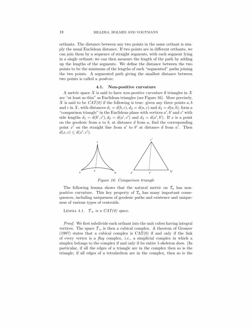
4.1. Non-positive curvatureA metric space X is said to have non-positive curvature if triangles in X

are “at least as thin” as Euclidean triangles (see Figure 16). More precisely,X is said to be CAT(0) if the following is true: given any three points a, band c in X, with distances d1 = d(b, c), d2 = d(a, c) and d3 = d(a, b), form a“comparison triangle” in the Euclidean plane with vertices a′, b′ and c′ withside lengths d1 = d(b′, c′), d2 = d(a′, c′) and d3 = d(a′, b′). If x is a pointon the geodesic from a to b, at distance d from a, find the correspondingpoint x′ on the straight line from a′ to b′ at distance d from a′. Thend(x, c) ≤ d(x′, c′).

a b

cc’

a’ b’xx’

Figure 16: Comparison triangle

The following lemma shows that the natural metric on Tn has non-positive curvature. This key property of Tn has many important conse-quences, including uniqueness of geodesic paths and existence and unique-ness of various types of centroids.

Lemma 4.1. T n is a CAT(0) space.

Proof. We first subdivide each orthant into the unit cubes having integralvertices. The space T n is then a cubical complex. A theorem of Gromov(1987) states that a cubical complex is CAT(0) if and only if the linkof every vertex is a flag complex, i.e., a simplicial complex in which asimplex belongs to the complex if and only if its entire 1-skeleton does. (Inparticular, if all the edges of a triangle are in the complex then so is thetriangle; if all edges of a tetrahedron are in the complex, then so is the


tetrahedron, and so on). Note that the link Ln of the origin, defined in theprevious section, is such a complex, since simplices are defined by pairwisecompatibility of partitions.

Let v be an arbitrary vertex of the cube complex, which lies in the interiorof a (unique) orthant of dimension k. This orthant corresponds to a treewith k interior edges, and thus to a set S of k pairwise compatible partitionsof {0, . . . , n}. If k is maximal, i.e., k = n−2, the link of v is a triangulatedsphere, which we think of as the k-fold suspension of the empty set. In gen-eral, the link of v is the k-fold suspension of the subcomplex of Ln spannedby all partitions compatible with S. Since this itself is a flag complex, andsince the suspension of a flag complex is again flag, this completes theproof.

Alternatively, T n is the 0-cone on the link Ln (for definition, see Bridsonand Haefliger (1999, I.5)). Since Ln is a flag complex, it is is CAT(1) byGromov’s theorem (Bridson and Haefliger (1999, 5.18,p. 211)). A theoremof Berestowski (Bridson and Haefliger (1999, 3.14, p. 188)) then impliesthat T n is CAT(0).

In the case n = 4, the flag condition says that the links of all verticesare graphs with no triangles; note that, for example, the smallest circuit inthe link of the origin has length 5. The fact that the set of unlabeled treesforms a flag complex was noted in (Billera et al., 1999).

4.2. GeodesicsSince the tree space T n is CAT(0), it follows by Gromov (1987) that

there is a unique shortest path connecting any two points of T n, called thegeodesic. In this section we characterize geodesics and show how to findthem. Once the geodesic is found, its length gives the distance between thetwo trees.

There is an obvious path between any two trees T and T ′ in T n, obtainedby connecting T to the origin by a straight line segment, then connectingthe origin to T ′ by another straight line segment; we will call this paththe cone path from T to T ′. The cone path may or may not be a geodesic,depending on the “angle” it makes at the origin T0. One makes this preciseas follows.

We have described the link of the origin in T n as the union of “flat” sim-plices, consisting of all points in each orthant with coordinate sum equal toone. We could just as well have considered each simplex as the intersectionof the unit sphere with the appropriate orthant, i.e., the set of points suchthat the sum of the squares of the coordinates is equal to one. This newmetric on simplices extends to a natural metric on the entire link Ln, inwhich each simplex is a right-angled spherical simplex with all edges oflength π/2. Each tree T of T n lies on a unique ray from the origin. Theintersection of this ray with Ln is called the projection of T onto Ln, and


is denoted t(T ). The angle between T and T ′, denoted 6 (T, T ′), is definedto be the distance between t(T ) and t(T ′) in the spherical metric on Ln.

Standard CAT(0) theory (see Bridson and Haefliger (1999), 5.6-5.10)tells us that the cone path is a geodesic if and only if the angle between Tand T ′ is at least π. If 6 (T, T ′) < π, the geodesic g from T to T ′ projectsto the unique geodesic γ from t(T ) to t(T ′) in Ln; furthermore, if we knowγ, we can reconstruct g.

Another standard notion we will need in this section is that of the de-velopment of a geodesic in a spherical complex (see Bridson and Haefliger(1999, p. 104), where the development of a geodesic is more generally de-fined). Let v be a vertex of Ln, and let γ be a geodesic in Ln starting at apoint t in the interior of a simplex in the star of v. If γ intersects a simplexσ in an arc of positive length, we say that γ traverses σ. Let σ1, σ2, . . . bethe sequence of simplices which γ traverses. For each i, γ intersects thecommon face σi ∩ σi+1 in a single point, which we will call ti. If t1 6= v,take the totally geodesic surface in σ1 containing t, v and t1; this surface isa spherical triangle τ1, with the distance of v to the other vertices equal toπ/2 (if we think of σ1 as lying in the unit sphere in a Euclidean orthant,this surface is the intersection of σ1 with the three-dimensional subspacecontaining these three points). We embed this triangle as a triangle τ1 inS2 with the image v of v at the north pole (see Figure 17).

v

τ1 τ2τ3

γ

t1

t2

t3

t

Figure 17: Development of γ on S2

If γ exits σ1 via a face with a vertex at v, we next take the totally geodesicsurface in σ2 containing v, t1 and t2; again this is a spherical triangle τ2which we embed in S2 as a triangle τ2 adjacent to τ1, with the image ofv at the north pole. We continue to lay out triangles in S2 as long asthe “exit faces” of γ have v as a vertex. The image γ of γ in S2 is calledthe development of γ near v, and is isometric to its preimage in γ. Recall


from Section 3 that each interior edge of a tree T partitions the leaves ofT into two sets, each with at least two elements. Edges of T and T ′ aresaid to be the same if they determine the same partition of the leaf-labels,and compatible if the corresponding partitions are compatible. A set ofpartitions corresponds to the set of interior edges of a tree if and only ifthe partitions are pairwise compatible.

Proposition 4.1. If the cone path from T to T ′ is not a geodesic, thenthere are non-empty sets E1 ⊃ E2 ⊃ . . . ⊃ Ek of the edges E(T ) of T , andF1 ⊂ F2 ⊂ . . . ⊂ Fk of the edges E(T ′) of T ′ such that(i) each element of Ei is compatible with each element of Fi, so that Ei∪Fiform the vertices of a simplex σi of Ln and(ii) the geodesic in Ln from t(T ) to t(T ′) traverses each simplex in thesequence σ1, . . . , σk.

Proof. Since the cone path is not a geodesic, the geodesic γ realizingthe distance between t(T ) and t(T ′) has length less than π.

Let σ be the simplex of Ln spanned by the edges E(T ). We first considerthe case that γ traverses σ. If γ is contained in the closure of σ, theproposition is trivial. If not, γ leaves σ via a face corresponding to a subsetof E(T ), which we define to be E1; this face is also a face of the nextsimplex σ1 which γ traverses.

Fix any vertex v in σ1 which is not in E1, and develop γ near v. Sinceγ has length less than π, the development γ remains in the northern hemi-sphere; this translates to the fact all simplices encountered by γ must havev as a vertex, including the simplex containing t(T ′), i.e., v corresponds toan edge of T ′. Since v was an arbitrary vertex of σ1 not in E1, the set ofvertices of σ1 consists of E1 plus a subset F1 of edges of T ′.

We now continue following the simplices traversed by γ, and repeat theargument to find vertex sets Ei and Fi as in the statement of the propositionuntil we arrive at the simplex containing t(T ′).

If γ does not traverse σ, we set E1 = E(T ), and let σ1 be the first sim-plex traversed by γ. We take any vertex v of σ1 which is not not in theface spanned by E1 and develop γ near v. We conclude that every simplexencountered by γ has v as a vertex, including the simplex containing t(T ′).Thus all vertices of σ1 which are not in E1 are in E(T ′), and we can set F1 tobe the vertices of σ1 not in E1. We now continue as before until we arrive att(T ′).

Corollary 4.1. If no edge of T is compatible with any edge of T ′, thenthe cone path is a geodesic.


Proof. If the cone path is not a geodesic, any element of F1 is compatiblewith any element of E1, by the proposition.

Example. The cone path may be a geodesic, even if T and T ′ do havesome compatible edges. For example, let T be the tree on four leaveswith edges e1 = {2, 3|0, 1, 4} and e2 = {1, 2, 3|0, 4}. and let T ′ be thetree with edges f1 = {0, 1|2, 3, 4} and f2 = {0, 1, 2|3, 4}. Then e1 and f1

are compatible. If the lengths of e1 and f1 are relatively large, then thegeodesic from T to T ′ passes through trees with edges {e1, f1}. However,if the lengths of e1 and f1 are small, the cone path will be a geodesic (seeFigure 18 ).

1 2 3 41

23

4

1 2 3 41 2 3 4

1 2 3 4

0 0

0

0

0

T

T'

f2

f1

e1

e2

Figure 18: Cone path may or may not be geodesic

Proposition 4.1 allows us to give an effective procedure for finding thegeodesic between binary trees T and T ′. We realize the orthants of T and T ′

as the totally negative and totally positive orthants of (n−2)−dimensionalEuclidean space Rn−2. We find all possible chains Ei and Fi as in thestatement of the proposition, find a candidate geodesic for each chain, andcompare their lengths. We carry out this procedure in Billera et al. (2001).

Suppose Ei has ni elements and Fi has mi elements. We order the edgesof T in such a way that edges in Ei correspond to the first ni coordinates ofRn−2 and edges in Fi correspond to the last mi coordinates. Our candidatefor the geodesic from T to T ′ is then a union of straight line segments inRn−2, constrained by the fact that each line segment must lie in one of theorthants whose first ni coordinates are negative, whose last mi coordinatesare positive, and whose remaining coordinates are zero. We illustrate thiswith the following special case:

Let T ∈ T n be a tree, and e an interior edge of T . We denote by |e|Tthe branch length of e in T .


Proposition 4.2. Let T and T ′ be binary trees with no edges in com-mon. Suppose the edges {ei} of T and {fi} of T ′ can be ordered in sucha way that Ei = {e1, . . . , ei} and Fi = {fi+1, . . . , fn−2} are compatible forall k = 1, . . . , n − 3. If for all i < j we have |ei|T |ej |T ′ − |ej |T |ei|T ′ > 0,then the geodesic from T to T ′ contains trees with edge sets Ei ∪ Fi forall i, and the distance from T to T ′ is the length of the vector (|e1|T +|e′1|T ′ , . . . , |en−2|T + |e′n−2|T ′).

Proof. The compatibility conditions say that the orthants correspond-ing to the trees Ti and Ti+1 share a codimension 1 face; in fact we mayarrange that the orthant for Ti is the orthant whose first n − 2 − i coor-dinates are negative and whose last i coordinates are positive. The treeT corresponds to the point (−|e1|T , . . . ,−|en−2|T ) and T ′ to the point(|e′1|T ′ , . . . , |e′n−2|T ′); the inequalities ensure that the straight line betweenthese two points is contained in the union of the orthants corresponding tothe Ti, which is therefore the geodesic from T to T ′.

The following corollary says that we can basically ignore edges of T andT ′ which are the same when we are computing the geodesic from T to T ′:

Corollary 4.2. Let e be an edge of T which is also an edge of T ′. Thenevery tree on the geodesic from T to T ′ has e as an edge.

Proof. The geometric meaning of this statement is that the union X(e)of the orthants containing the ray R(e) corresponding to e is convex in T n.

Since R(e) is an edge of the orthant containing T , the angle betweenR(e) and T is less than π/2. Since the orthants containing T and T ′

intersect in R(e), the angle between T and T ′ is less than π, so thatthe cone path is not a geodesic. Consider the geodesic γ in the link Lnfrom t(T ) to t(T ′). By Proposition 4.1, every edge in every simplex tra-versed by γ is compatible with e, i.e., γ stays in the closed star of thevertex v(e) corresponding to e. If we develop γ near v(e), it begins andends in the open northern hemisphere, so remains in the open northernhemisphere at all times. This translates to the fact that every simplexencountered by γ in fact has v(e) as a vertex, as we wished to show.

For any edge e, the union X(e) of quadrants containing the ray R(e) isa product [0,∞) × C(e), where C(e) is a cone on the flag complex of allsets of partitions which are compatible with e. The cone C(e) is thus alsoa CAT(0) complex, consisting of a union of orthants sharing a commonorigin. The geodesic from T to T ′ projects to a geodesic in C(e); in fact, ifwe know the geodesic from the projections of T and T ′ onto C(e), we can


recover the geodesic from T to T ′ by following this geodesic while rescalingthe length of e linearly from |e|T to |e|T ′ .

We conclude this section with an easily checked criterion which is suffi-cient to show that the cone path is not a geodesic:

Notation. Let T ∈ T n be a tree, and e an interior edge of T . The norm‖T‖ is the Euclidean length of the vector of branch lengths of edges of T ,(i.e., the square root of the sum of the squares of the branch lengths).

Let E = {e1, . . . , ek} be a set of edges of T ; we denote by T (E) the treewith edge set exactly E, with branch lengths inherited from T . We mayalso think of T (E) as obtained from T by collapsing every edge not in E.We denote by T/E the tree obtained from T by collapsing every edge in E.

Proposition 4.3. Suppose that T and T ′ have no edges in common, butthat a set of edges E = {e1, . . . , ek} of T is compatible with a set of edgesF = {f1, . . . , fl} of T ′, and that ‖T (E)‖‖T ′(F )‖ − ‖T/E‖‖T ′/F‖ > 0.Then the cone path is not a geodesic.

Proof. Informally, the inequality ensures that we can produce a shorterpath than the cone path by “cutting across” the orthant corresponding tothe tree with edge set exactly E∪F . Formally, we show that 6 (T, T ′) is lessthan than π, and hence that the cone path is not a geodesic by Gromov’scriterion (Gromov (1987)).

Since T and T (E) are in the same quadrant, the angles α = 6 (T, T (E))is at most π/2; similarly, and β = 6 (T ′, T ′(F )) ≤ π/2. Since E and F aredisjoint but compatible, 6 (T (E), T ′(F )) = π/2.(see Figure 19)

T'

T

α T(e)

T(f) β

Figure 19: The cone path from T to T ′


The angle between T and T ′ is at most α+π/2+β. Therefore 6 (T, T ′) <π if α+ β < π/2, i.e., if cos(α+ β) > 0. We have

cos(α+β) = cos(α) cos(β)−sin(α) sin(β) =‖T (E)‖‖T‖

‖T ′(F )‖‖T ′‖ −

‖T/E‖‖T‖

‖T ′/F‖‖T ′‖ ,

which is positive if and only if ‖T (E)‖‖T ′(F )‖ − ‖T/E‖‖T ′/F‖ > 0.

4.3. CentroidsThere are several ways of defining the center of a finite scatter of points X

in a CAT(0) metric space, including the center of mass, the circumcenter,and the points of maximum depth. The center of mass, defined for anyprobability distribution over the space, is the unique point that minimizesthe expected squared distance from points in the space (see §3.2 in Jost(1997)). To define the center of mass of a finite point set, we take theuniform distribution over X. A clear account of this type of mean valueand its properties can be found in Sturm (2000a,b). Another type of center,the circumcenter, is the center of the smallest ball enclosing the points ofX (see, e.g. Brown (1989)). The points of maximum depth (Tukey (1975))are defined by forming the convex hull of X (i.e., the smallest set containingX and containing all geodesic paths between pairs of its points), removingthe extreme points (the minimal subset of X having the same convex hull)and repeating until the set becomes empty.

In this section we introduce another notion of center, which we call thecentroid. The centroid of a set of n > 2 points is defined by iteratingthe operation of taking centroids of each subset of n − 1 points, wherethe centroid of 2 points is defined to be the midpoint of the geodesic paththat joins them. We note that for n = 3, our construction gives the samecentroid as that defined in Bruhat and Tits (1972, pp. 63-64).

It should be noted that to compute any of these notions of center for afinite set of points in a CAT(0) space X, one needs to be able to computethe geodesic paths between pairs of points, as discussed in the previoussection for the space T n.

For x, y ∈ X, let c({x, y}) denote the midpoint of the (unique) geodesicjoining x to y. Suppose Y ⊂ X is a set with n > 2 elements (some of whichmay be repeated), and suppose we have defined c(W ) for all W ⊂ X with|W | < n. Then let c1(Y ) denote the set { c(W ) | W ⊂ Y, |W | = n − 1 },and for k > 1, ck(Y ) = c1(ck−1(Y )). Note that the sets ck(Y ) all have nelements (some possibly repeated).

We begin by observing that for Euclidean spaces, the sets ck(Y ) can beused to find the usual centroid c(Y ) = 1

|Y |∑y∈Y y of any finite set Y . It is

straightforward to check in this case that c(Y ) = c(c1(Y )), and if |Y | = n,diam c1(Y ) = 1

n−1 diam c(Y ). From this the following is immediate.


Proposition 4.4. If X is a subset of a Euclidean space and c(W ) de-notes the centroid of W , then for any finite subset Y ⊂ X, the elements inck(Y ) converge to the point c(Y ) ∈ X as k →∞.

Our goal is to prove that the convergence in Proposition 4.4 continuesto hold in an arbitrary CAT(0) space; the resulting limit point c(Y ) willbe defined to be the centroid of the set Y . To do this we need to prove ageneral form of the convexity property that essentially defines these spaces.Suppose centroids exist for all n-element subsets of a CAT(0) space X. Wesay the centroid function c(Y ) is convex if whenever Y = {y1, . . . , yn} andY ′ = {y′1, . . . , y′n}, then d(c(Y ), c(Y ′)) ≤ 1

n

∑d(yi, y′i).

Theorem 4.1. In any CAT(0) space X,

1.centroids exist for any finite set Y ⊂ X, and2.the centroid function is convex.

Proof. The proof is by induction on n = |Y |. The case n = 2 isProposition II.2.2 in Bridson and Haefliger (1999).

Suppose n ≥ 3 and we have a convex centroid function c(W ) for |W | =n−1. Let Y = {y1, . . . , yn} and Yi = Y \{yi}. Suppose Y has diameter D.Then by convexity for (n−1)-sets, d(c(Yi), c(Yj)) ≤ 1

n−1 d(yi, yj) ≤ 1n−1D,

and so diam c1(Y ) ≤ 1n−1D. Thus the diameter of ck(Y ) is bounded above

by(

1n−1

)kD and so goes to zero.

To show convergence, let Dk denote the diameter of ck(Y ), and considerthe sequence zk ∈ ck(Y ), where z0 = y1, z1 = c(Y1), z2 = c({c(Yi) : i 6= 1}),etc. It follows by convexity for (n−1)-sets that d(zk, zk+1) ≤ 1

n−1Dk. Thusfor l ≥ k,

d(zk, zl) ≤ Dk +1

n− 1Dk +

(1

n− 1

)2

Dk + · · · =n− 1n− 2

Dk,

showing that {zk} is a Cauchy sequence. Thus, centroids exist for n-sets.To show convexity of c(Y ), |Y | = n, suppose Y = {y1, . . . , yn} and

Y ′ = {y′1, . . . , y′n}. If Yi = Y \ {yi} and Y ′i = Y ′ \ {y′i}, then by convexityfor (n− 1)-sets,

d(c(Yi), c(Y ′i )) ≤ 1n− 1

∑j 6=i

d(yj , y′j) (1)

for each i. Let δi = d(yi, y′i) and d0 = (δ1, . . . , δn). Then if dk is thecorresponding vector of distances between elements of ck(Y ) and ck(Y ′),


it follows from (1) that dk ≤ Bknd0, where Bn = 1n−1 (Jn − In), Jn is the

n × n matrix of 1′s and In is the n × n identity matrix. Since Bkn →1nJ as k →∞, it follows that d(c(Y ), c(Y ′)) ≤ 1

n

∑d(yi, y′i) as desired.

Since T n is a CAT(0) space, any finite set of points has a unique centroid.If the points are all in the same orthant, i.e., correspond to trees withthe same combinatorial structure but possibly different branch lengths,then the centroid is the usual Euclidean centroid of the points, i.e., itcorresponds to the tree with the given combinatorial structure and theaverage of the branch lengths (see Proposition 4.4).

If two trees have all branch lengths equal to 1 but have no combinatorialstructure in common, the centroid will be the origin, i.e., the tree with allbranch lengths equal to 0. In a large set which contains one tree which ismarkedly different from the others, the effect of this tree on the centroidwill be negligible. An interesting effect occurs when there are duplicatetrees in the set. We illustrate this by the following example: Let T1, T2 andT3 be the trees illustrated in Figure 20.

1 42 3

0

13

2 4

0

21 43

0

1 11

1

32

Figure 20: Three trees

The centroid of {T1, T2, T3} is the left tree in Figure 21, while the centroidof {T1, T1, T2, T2, T3, T3} is the tree on the right. This shows a non-linearproperty of this definition of centroid.

1 32 4

0

1

1/3

1 32 4

0

1

2/5

Figure 21: Two different centroids

This method of taking centroids provides a coherent mathematical wayof forming the consensus of a set of trees. The convexity property of cen-troids says that given two sets {T1, . . . , Tk} and {T ′1, . . . , T ′k} of trees, thedistance between the centroids will be less than or equal to the average of


the distances from Ti to T ′i . Thus taking centroids of the two sets createstwo trees which agree at least as well as the average pairwise agreement.

4.4. Probability Measures on Tree SpaceAldous (1996) has described several possible constructions for probabil-

ity measures on combinatorial trees without branch lengths. One of theparameters he proposes to use is the height of the tree, which is defined asthe largest number of interior edges between a leaf and the root.

There are several natural routes to complementing our geometric con-struction with a probability measure. They are all simplified by imposinga bound on the interior branch lengths. This has the effect of truncatingeach orthant to a cube.

In this section we assume the branch lengths are renormalized, to obtainunit cubes. The extension to more general compact subsets of tree spaceis straightforward. Here are some natural measures:

• The base measure called dτ puts a probability of 1/(2n− 3)!! on eachcube, while within the cube the distribution is considered uniform. Notethat balls of the same radius centered at different points may have differentprobabilities. It is clear that for τ far from any of the boundary regions (i.e.,equivalently all the edges of τ sufficiently large), dτ will be proportionalto the volume of a small cube around τ . In this case dτ denotes the localLebesgue measure in the cube.

If τ is a metric binary tree with exactly one small edge, then its neighbor-hood will meet 3 cubes. If the number of small edges is k there will be atmost (2k + 1)!! neighboring cubes for τ .

For trees with n leaves, the maximum volume attained is at the origin,which is contained in 2(n− 3)!! cubes.• If one wants to describe the simple case of a distribution concentrated

around a center, then a probability distribution can be defined using thenotion of distance we have developed above. This follows a Mallows’ typemodel as developed for the symmetric group in (Mallows (1957), Diaconis(1988)) or for decision trees in Shannon and Banks (1999). In this model thecentral tree τ0 together with an exponential family produces a probabilityfor any branching pattern τ , defined by

f(τ) = Ke−λd(τ,τ0)dτ.

The term K is a normalizing constant and λ is a concentration param-eter; for λ = 0 the distribution is the base measure, and as λ increasesthe measure will be more concentrated around τ0. This is a distributionconcentrated around the central element τ0, which we can choose to be thecentroid that we defined in section 4.3.


• Non-uniform probabilities can be constructed to agree with some infor-mation about the data; for example if one wants to be nearly sure to have abinary tree, without knowing which tree, each orthant could be given mea-sure 1/(2n− 3)!!, but the distribution on each cube could be concentratedat the point with all branch lengths equal to 1.

Remarks:

1. In the case when the parametric maximum likelihood method hasbeen used to determine the optimal tree, there is a natural measure onT n that will result in likelihood-based confidence regions. This supposesa parametric mutation model. An example of this is provided in Billeraet al. (2001).

2. Eventually our aim is to be able to map a probability on to the spaceso we can create isocontours determining confidence regions. Maybe a goodintuitive picture is:

Figure 22: A hot plot of a possible probability

5. REAL DATA EXAMPLE

In this section we illustrate how the questions of averaging trees andbuilding confidence regions in tree space come about, by examining a realdata set. This data set consists of 12 mitochondrial DNA sequences, each


of length 898 bases, from 12 species of primates. This data is publishedin Hayasaka et al. (1988). We will use the program dnapars, from Felsen-stein’s Phylip package (available on his web site Felsenstein (1993)) to findthe most parsimonious trees for these DNA sequences.

The following list shows the species names, in quotes, together with thefirst 80 characters of our DNA data. Data are collected by reading theDNA sequences for a specific gene occurring in all of the species. Thesesequences are written in rows, and the rows undergo a multiple alignmentso that they have the greatest possible agreement in the columns. Here ispart of the data:

’Lemur_catta’ AAGCTTCATAGGAGCAACCATTCTAATAATCGCACATGGCCTTACATCATCCA...

’Tarsius_syrichta’AAGTTTCATTGGAGCCACCACTCTTATAATTGCCCATGGCCTCACCTCCTCCC...

’Saimiri_sciureus’AAGCTTCACCGGCGCAATGATCCTAATAATCGCTCACGGGTTTACTTCGTCTA...

’Macaca_sylvanus’ AAGCTTCTCCGGTGCAACTATCCTTATAGTTGCCCATGGACTCACCTCTTCCA...

’Macaca_fascicul.’AAGCTTCTCCGGCGCAACCACCCTTATAATCGCCCACGGGCTCACCTCTTCCA...

’Macaca_mulatta’ AAGCTTTTCTGGCGCAACCATCCTCATGATTGCTCACGGACTCACCTCTTCCA...

’Macaca_fuscata’ AAGCTTTTCCGGCGCAACCATCCTTATGATCGCTCACGGACTCACCTCTTCCA...

’Hylobates’ AAGCTTTACAGGTGCAACCGTCCTCATAATCGCCCACGGACTAACCTCTTCCC...

’Pongo’ AAGCTTCACCGGCGCAACCACCCTCATGATTGCCCATGGACTCACATCCTCCC...

’Gorilla’ AAGCTTCACCGGCGCAGTTGTTCTTATAATTGCCCACGGACTTACATCATCAT...

’Pan’ AAGCTTCACCGGCGCAATTATCCTCATAATCGCCCACGGACTTACATCCTCAT...

’Homo_sapiens’ AAGCTTCACCGGCGCAGTCATTCTCATAATCGCCCACGGGCTTACATCCTCAT...

The program dnapars found two different trees, each with total branchlength 1163,meaning that 1163 mutations are needed to explain the DNAsequences in each tree (see Figure 23). We note that the situation of theroot is unspecified a priori; however, it is known in this case to be at theLemur branch as depicted. Simple inspection of the two trees shows thatonly one of its aspects seems subject to be in doubt, namely the branchingbetween Pan, Gorilla and Homo sapiens.


Homosapien

Pan

Gorilla

Pongo

Hylobates

Macaca_fus

Macaca_mul

Macaca_fas

Macaca_syl

Saimiri_sc

Tarsius_sy

Lemur_catt

Figure 23: First tree

Homosapien

Pan

Gorilla

Pongo

Hylobates

Macaca_fus

Macaca_mul

Macaca_fas

Macaca_syl

Saimiri_sc

Tarsius_sy

Lemur_catt

Figure 24: Second tree

Thus the relevant confidence statement says that we are ‘sure’ of allparts of the tree except for the relationship between Homosapiens, Pan andGorilla. Either the first two are together or the latter two are together.Only two of the three possible subtrees with three branches are equallylikely; thus a confidence region assigning equal probabilities to each ofthese two in a continuous way would be reasonable if no other informationwere available.

The fact that two different trees were produced is a result of conflicts inthe data. Biologists often translate such contradictions by saying that thetree has an unresolved node and using a triple branch at this node, withhomo sapiens, gorilla and pan all descended from a single ancestor, withno chosen two-some apparent among them. Note that the centroid of thetwo trees in the sense of section 4.3 in tree space is on the boundary linerepresented by the same unresolved tree. Thus here our notion of centroidgives a triple branch at the disputed node with homo sapiens, gorillaand pan all coming from a common ancestor, which is the same as therepresentation of uncertainty that the biologists use.

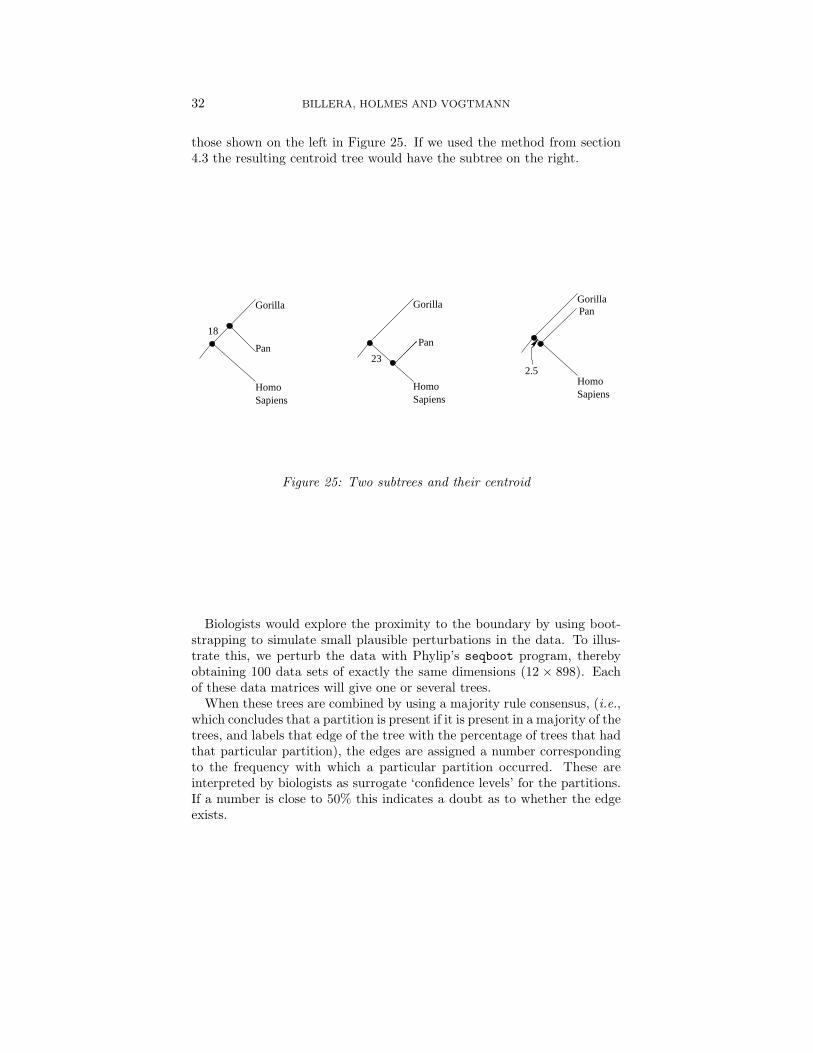
If the proportions were not fifty-fifty we would get a binary tree withnon-zero edge lengths. For instance if we assigned a biological meaning tothe edge lengths, such as the number of mutations along that branch, thenthe respective lengths given by dnapars on the relevant subtrees would be


those shown on the left in Figure 25. If we used the method from section4.3 the resulting centroid tree would have the subtree on the right.

18

Pan

HomoSapiens

Gorilla

HomoSapiens

Gorilla

Pan

23

HomoSapiens

GorillaPan

2.5

Figure 25: Two subtrees and their centroid

Biologists would explore the proximity to the boundary by using boot-strapping to simulate small plausible perturbations in the data. To illus-trate this, we perturb the data with Phylip’s seqboot program, therebyobtaining 100 data sets of exactly the same dimensions (12 × 898). Eachof these data matrices will give one or several trees.

When these trees are combined by using a majority rule consensus, (i.e.,which concludes that a partition is present if it is present in a majority of thetrees, and labels that edge of the tree with the percentage of trees that hadthat particular partition), the edges are assigned a number correspondingto the frequency with which a particular partition occurred. These areinterpreted by biologists as surrogate ‘confidence levels’ for the partitions.If a number is close to 50% this indicates a doubt as to whether the edgeexists.


Homosapien

Pan

Gorilla

Pongo

Hylobates

Macaca_fus

Macaca_mul

Macaca_fas

Macaca_syl

Saimiri_sc

Tarsius_sy

Lemur_catt

50.2

100.0

89.0

79.4

99.0

100.0

99.5

100.0100.0

100.0

Figure 26: Tree with confidence levels

Such an edge-weighted tree is unsatisfactory as a summary of the per-turbation analysis. A multidimensional representation would be more in-formative. The embedding property of the tree space will often make sucha representation feasible in practice, at least approximately. In the case ofFigure 26 the only notable differences that occur are on 3 edges. We canproject all the trees onto a complex of three-dimensional cubes. Lookingat the data this way, it is possible to further simplify since for instance thecube with the edge corresponding to the grouping of homo sapiens andgorilla does not exist. A more detailed analysis of such examples can befound in Billera et al. (2001).

References

D. Aldous. Probability distributions on cladograms. In David Aldousand Robin Pemantle, editors, Random discrete structures, pages 1–18.Springer, New York, 1996.

V. Berry and O. Gascuel. Interpretation of bootstrap trees : threeshold ofclade selection and induced gain. Molecular Biology and Evolution, 13:


999–1011, 1996.L. Billera, C. Chan, and N. Liu. Flag complexes, labelled rooted trees,

and star shellings. In B. Chazelle. J.E. Goodman and R. Pollack, editors,Advances in discrete and computational geometry, pages 91–102. A. M.S., Providence, RI, 1999.

L. Billera, S. Holmes, and K. Vogtmann. A geometrical perspective onthe phylogenetic tree problem. Technical report, Statistics, Sequoia Hall,Stanford, CA 94305, 2001.

S. Bocker and A. W. M. Dress. Recovering symbolically dated, rootedtrees from symbolic ultrametrics. Adv. Math., 138(1):105–125, 1998.

M.R. Bridson and A. Haefliger. Metric spaces of non-positive curvature.Grundlehren der math Wiss. Springer Verlag, 1999.

D. R. Brooks. Hennig’s parasitological method: A proposed solution. Syst.Zool., 30:229–249, 1981.

K.S. Brown. Buildings. Springer Verlag, 1989.F. Bruhat and J. Tits. Groupes reductifs sur un corps local. Institut des

Hautes Etudes Scientifiques, 41:5–252, 1972.M. Davis, T. Januszkiewicz, and R. Scott. Nonpositive curvature of blow-

ups. Selecta Math. (New Series), 4(4):491–547, 1998.S. L. Devadoss. Tessellations of moduli spaces and the mosaic operad. In

Homotopy invariant algebraic structures (Baltimore, MD, 1998), pages91–114. Amer. Math. Soc., Providence, RI, 1999.

P. Diaconis. Group representations in probability and statistics. Instituteof Mathematical Statistics, Hayward, CA, 1988.

P. Diaconis and S. Holmes. Matchings and phylogenetic trees. Proc. Natl.Acad. Sci. USA, 95(25):14600–14602 (electronic), 1998.

J.J. Doyle. Gene trees and species trees: Molecular systematics as one-character taxonomy. Syst. Bot., 17:144–163, 1992.

H. Edelsbrunner. Algorithms in Combinatorial Geometry. Springer Verlag,1987.

B. Efron, E. Halloran, and S. Holmes. Bootstrap confidence levels forphylogenetic trees. Proc. Natl. Acad. Sci. USA, 93:13429–34, 1996. ISSN1091-6490.

A. Escalante and F. Ayala. Phylogeny of the malarial genus plasmodiumderived from rrna gene sequences. Proc. Nat. Ac. Sciences, 91:11371–11377, 1995.

J. Felsenstein. Statistical inference of phylogenies (with discussion). Jour-nal Royal Statistical Society A, 146:246–272, 1983.

J. Felsenstein. PHYLIP, (Phylogeny Inference Package)version 3.5c. Department of Genetics, University ofWashington, Seattle, version 3.5c. edition, 1993. URLhttp://evolution.genetics.washington.edu/phylip.html.


L. R. Foulds and R. L. Graham. The Steiner problem in phylogeny isNP-complete. Adv. in Appl. Math., 3(1):43–49, 1982.

M. Gromov. Hyperbolic groups. In Essays in group theory, pages 75–263.Springer, New York, 1987.

E. Haeckel. Generelle Morphologie der Organismen: AllgemeineGrundzuge der organischen Formen-Wissenschaft, mechanisch begrun-det durch die von Charles Darwin, reformite Descendenz-Theorie. GeorgRiemer, Berlin, 1866.

K. Hayasaka, T. Gojobori, and S. Horai. Molecular phylogeny and evolu-tion of primate mitochondrial dna. Mol. Biol. Evol., 5/6:626–644, 1988.

S. Holmes. Phylogenetic trees: an overview. In Statistics and Genetics,number 112 in IMA, pages 81–118. Springer, New York, 1999.

J. Jost. Nonpositive curvature: Geometric and Analytic Aspects. Lecturesin Mathematics ETH Zurich. Birkhauser Verlag, 1997.

M. M. Kapranov. The permutoassociahedron, Mac Lane’s coherence the-orem and asymptotic zones for the KZ equation. J. Pure Appl. Algebra,85(2):119–142, 1993.

J. Krushkal and W.H. Li. Evolution of primate immunodeficiency viruses.In P. Auger and R. Jean, editors, Advances in Mathematical PopulationDynamics- Molecules, Cells and Man, pages 5–24. World scientific, 1998.

C.W. Lee. The associahedron and triangulations of the n-gon. Europ. J.Combinatorics, 10:551–560, 1989.

J. Lin and M. Gerstein. Whole genome trees based on the occurrenceof folds and orthologs: implications for comparing genomes on differentlevels,. Genome Research, 10(6):808–818, 2000.

L. Lovasz and M. D. Plummer. Matching Theory. North Holland, Ams-terdam, 1985.

B.J. MacFadden. Patterns of phylogeny and rates of evolution in fossilhorses: Hipparions from the Miocene and Pliocene of North America.Paleobiology, 1(3):245–257, 1985.

C. L. Mallows. Non-null ranking models. I. Biometrika, 44:114–130, 1957.A. Robinson and S. Whitehouse. The tree representation of σn+1. J. Pure

Appl. Algebra, 111(1-3):245–253, 1996.E. Schroder. Vier combinatorische probleme. Zeit. fur Math. Phys., 15:

361–376, 1870.W. Shannon and D. Banks. Combining classification trees using maximum

likelihood estimation. Statistics In Medicine, 18:727–740, 1999.D. D. Sleator, R. E. Tarjan, and W. P. Thurston. Rotation distance,

triangulations, and hyperbolic geometry. J. Amer. Math. Soc., 1(3):647–681, 1988.

D. D. Sleator, R. E. Tarjan, and W. P. Thurston. Short encodings ofevolving structures. SIAM J. Discrete Mathematics, 5(3):428–450, 1992.


R. Stanley. Enumerative Combinatorics. Cambridge University Press,1999.

J.D. Stasheff. Homotopy associativity of h-spaces i. Trans. Amer. Math.Soc., 108:275–292, 1963.

K. T. Sturm. Nonlinear markov operators, discrete heat flow, andharmonic maps between singular spaces. Preprint from http://www-wt.iam.uni-bonn.de/homepages/sturm/sturm.html, 2000a.

K. T. Sturm. Nonlinear martingale theory for processes with valuesin metric spaces of nonpositive curvature. Preprint from http://www-wt.iam.uni-bonn.de/homepages/sturm/sturm.html, 2000b.

J.W. Tukey. Mathematics and the picturing of data. In Proceedings ofthe International Congress of Mathematicians, volume 2, pages 523–531,Vancouver, 1975.

K. Vogtmann. Local structure of some out(Fn)-complexes. Proc. Edin-burgh Math. Soc. (2), 33(3):367–379, 1990.

M. S. Waterman and T. F. Smith. On the similarity of dendrograms. J.Theoret. Biol., 73(4):789–800, 1978.

A. Zharkikh and W.H. Li. Estimation of confidence in phylogeny: Thecomplete and partial bootstrap technique. Mol. Phylogenet. Evol., 4:44–63, 1995.

ACKNOWLEDGMENTSWe thank Martin Bridson, Persi Diaconis, Laurent Saloff-Coste, Richard Stanley

and Tom Zaslavsky for helpful discussions and an anonymous referee for constructivecomments.

geometry of the space of phylogenetic treesfinmath.stanford.edu/~susan/papers/lap.pdf · geometry...

Documents