geophone azimuth consistency from calibrated vertical ... · geophone azimuth consistency ......

Geophone azimuth consistency

CREWES Research Report — Volume 23 (2011) 1

Geophone azimuth consistency from calibrated vertical seismic profile data

Peter Gagliardi and Don C. Lawton

ABSTRACT Raw borehole geophone data, taken from a 3-line walkaway vertical seismic profile

(VSP) acquired in the Pembina oil field in Alberta, was examined for orientation azimuth consistency. Data were recorded using a 16-level VSP tool placed at three different levels in a deviated well. An algorithm was developed that compensated for the added complexities of a deviated well. Orientation azimuths, using all three lines, had an average standard deviation of 4.39°; consistency was poorest for the mid-level tool position, and best for the shallow-level tool position. Most interestingly, orientation azimuths calculated using sources from Line 1 were, on average, 3.7° higher than Line 2 and 3.0° higher than Line 6. This was judged to be related to geological properties of the area, particularly azimuthal anisotropy.

INTRODUCTION In 2007, a walkaway vertical seismic profile (VSP) survey was acquired in the

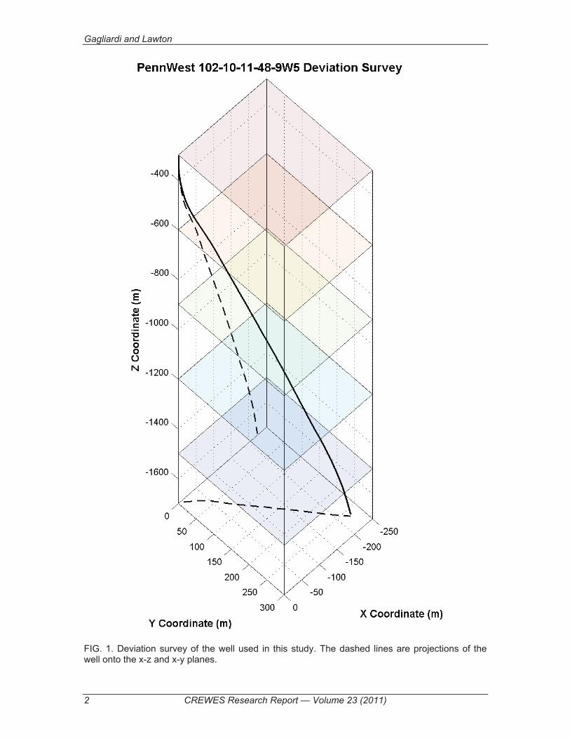
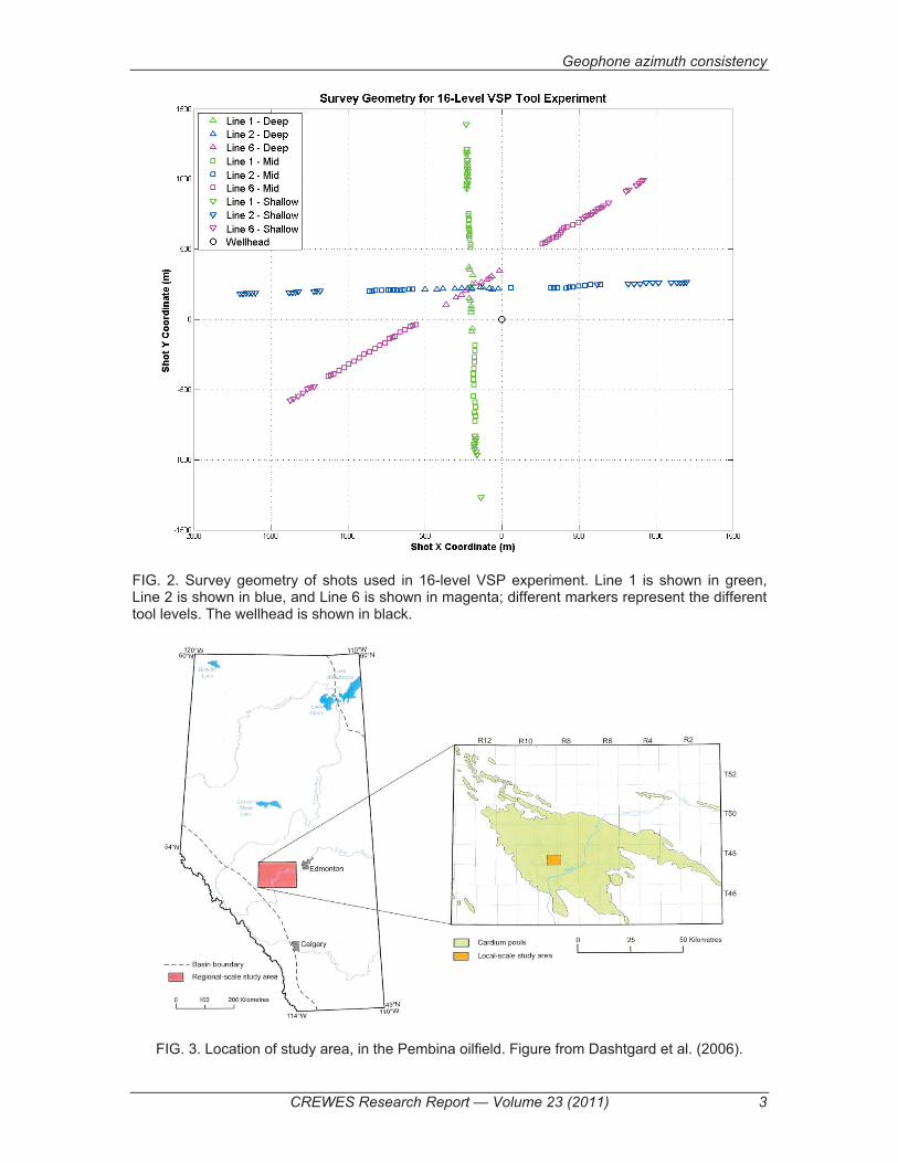
Pembina field, near Violet Grove, Alberta. The well used was PennWest 102-10-11-48-9W5 (Figure 1), which had a maximum deviation of 17� and a total depth of 1644 m. A 16-level VSP tool was used to record the survey, placed at 3 different depth ranges in the well: 798 – 1025 m (shallow), 1038 – 1265 m (mid), and 1278 – 1505 m (deep). The receiver spacing was 15.12 m. Shots were taken along 3 2D lines at a variety of offsets, ranging from 200 – 1700 m, using dynamite as a source (Figure 2). Since VSP tools tend to rotate when they are placed in a well, their exact orientation azimuth is initially unknown; this is especially troublesome if the receivers are going to be used to locate microseismic events such as hydraulic fractures. In this project, the orientation azimuths of the receivers in the tool were determined from first arrival analysis and were examined for consistency.

STUDY AREA The Pembina CO2 monitoring pilot has produced a wealth of interesting information

regarding many geophysical and geological concepts, including CO23

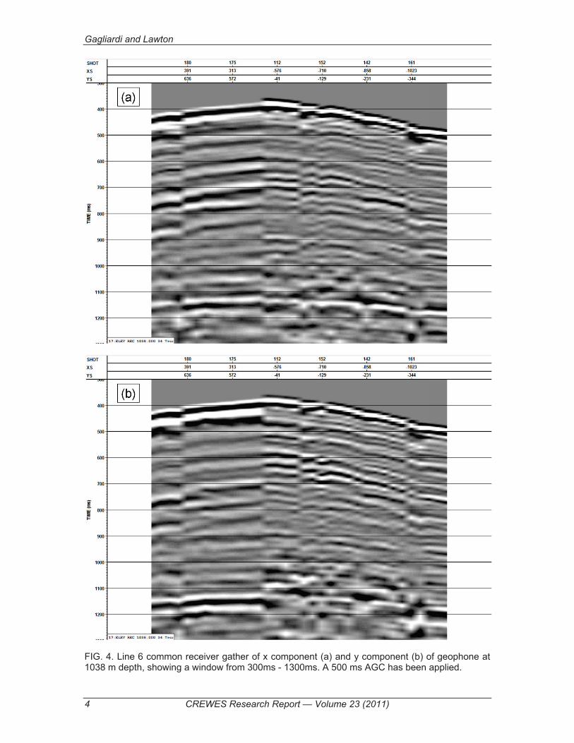
sequestration time-lapse geophysics. The Pembina oilfield (Figure ) is just over 100 km southwest of Edmonton and its major pool, in the Cardium, is the largest conventional oil pool that has been discovered in Western Canada (Hitchon, 2009). The seismic surveys acquired over the course of this project consisted of four 2D lines: two parallel, east-west trending lines (Lines 2 and 3), a line trending southwest-northeast (Line 6) and finally, a north-south line (Line 1); the source used for all lines was dynamite. Lines 1, 2 and 6 are used in this study. Some of the raw x and y-component data are shown side-by-side in Figure 4.

Gagliardi and Lawton

2 CREWES Research Report — Volume 23 (2011)

FIG. 1. Deviation survey of the well used in this study. The dashed lines are projections of the well onto the x-z and x-y planes.



FIG. 2. Survey geometry of shots used in 16-level VSP experiment. Line 1 is shown in green, Line 2 is shown in blue, and Line 6 is shown in magenta; different markers represent the different tool levels. The wellhead is shown in black.

FIG. 3. Location of study area, in the Pembina oilfield. Figure from Dashtgard et al. (2006).



FIG. 4. Line 6 common receiver gather of x component (a) and y component (b) of geophone at 1038 m depth, showing a window from 300ms - 1300ms. A 500 ms AGC has been applied.



ROTATION METHODS Vertical Well

The algorithm used to calculate the source-receiver rotation angle was (DiSiena et al., 1984)

tan 2� = ��, (1)

where X and Y are the horizontal component data, � is the angle between the x-component (H1) and the source, and � is a crosscorrelation operator. In this case, horizontal data were windowed using a 100 ms window beginning at the first break. In order to facilitate an analysis encompassing all shots, the calculated rotation angle then needed to be converted into an azimuth measured from a common reference frame. For a vertical well, this can be achieved using

� = � + �, (2)

where � is the source-receiver azimuth and � is the receiver orientation azimuth, both relative to North. Since the well is vertical, we can assume that the horizontal components of the borehole geophones will be oriented on a plane parallel to the x-y plane; thus, when examining the source-receiver azimuth, it is sufficient to precisely use the x and y coordinates of the source location; that is,

� = arctan�� . (3)

Additionally, since Equation 1 will only produce angles between ± 90°, there will be two potential receiver trends separated by 180�; this is remedied by simply examining the polarity of the first breaks.

Deviated Well Now, let us consider an observation well that has an arbitrary deviation. At any point

along the well, particularly at a receiver location, we may consider a line �� tangent to the deviation. Using spherical coordinates, this can be expressed parametrically as

�� = �sin �� cos��sin �� sin��cos �� + �� , (4)

where �� is the well inclination angle, �� is the horizontal direction of the well relative to the positive x-axis, and xr, yr, zr are the coordinates of the receiver. Note that the signs of �� and zr must be carefully considered to be consistent with the coordinate system used. Using the direction of ��, we can define the normal to a plane that is perpendicular to the well at this point; that is,



�� = �sin �� cos��sin �� sin��cos �� . (5)

Finally, we must choose a useful coordinate system for this plane; for this study, the choice will be defined such that the new y-axis points directly up towards the surface. The new “pseudo” x and y axes are then defined as

�� = �� sin��cos��0 �; (6)

and

�� = �� cos �� cos�� cos �� sin��sin �� . (7)

It should be noted that these two vectors, along with the normal defined in Equation 5, provide a suitable vector basis for the analysis (Appendix A). In order to perform analysis of geophone orientation, we must now project the source coordinates onto the plane defined above. Given source coordinates xs, ys and zs

�� = �� ; (8)

, this can be done simply by calculating

and

� = �� , (9)

where �� is the source pseudo x coordinate, and � is the source pseudo y coordinate. We can now define a source-receiver azimuth using the projected source coordinates such that

�� = arctan�� . (10)

Finally, substituting � for �� in Equation 2 will give us a proper receiver orientation azimuth relative to ��. Note that Equations 4 through 10 will properly yield Equation 3 in the case of a vertical well (i.e. �� = 0°, �� is chosen to be -90°).

RESULTS The projected geometry of the Violet Grove survey, using pseudo x and y coordinates,

is shown in Figure 5. Linear interpolation was used in order to estimate the well inclination and azimuth at each receiver. It should be noted that the deviation survey was slightly different at each receiver; hence, each source had multiple projections. Receiver orientation azimuths between the x-component (H1) and pseudo y-axis were calculated



for Lines 1, 2 and 6. These angles were then plotted against source pseudo offset in order to judge the consistency of calculations (Figures 6-11); several trends are noticeable from these plots. First, as was noted in Gagliardi and Lawton (2010), increasing geophone depth results in increased scatter in the angle, if we consider each line separately. More interestingly, however, is the clear separation of the trends of each line, especially evident in the shallow-level tool position (Figures 6 and 7).

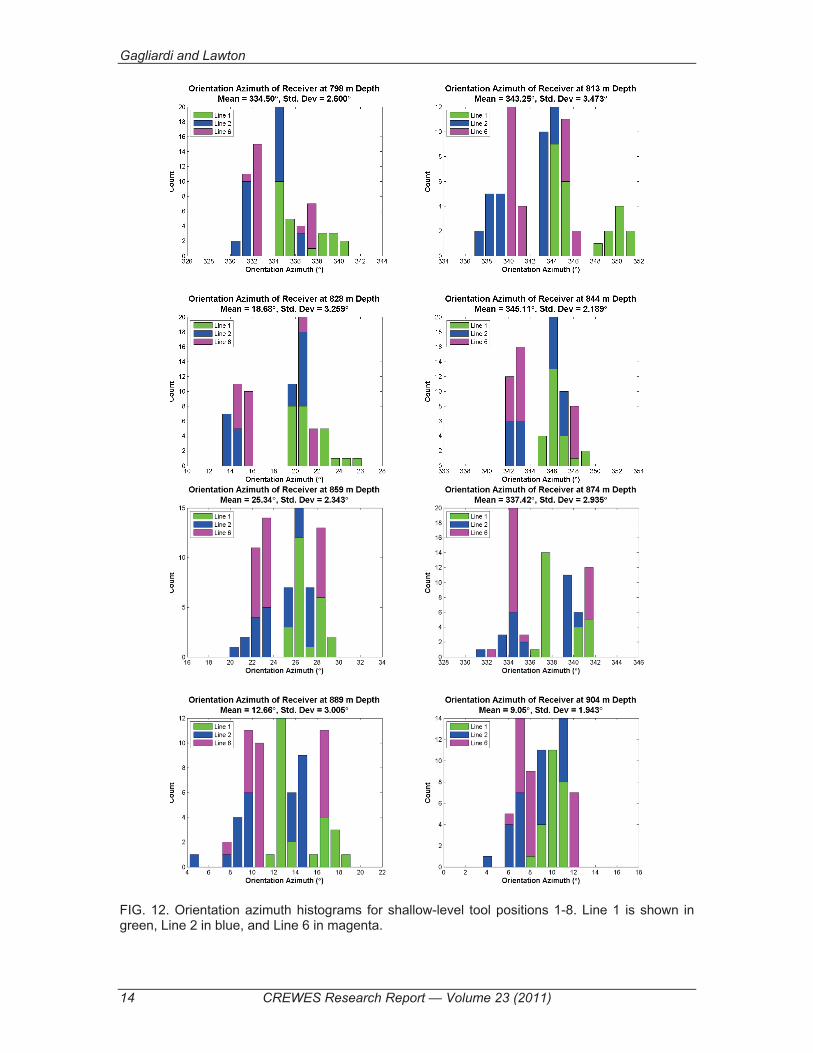
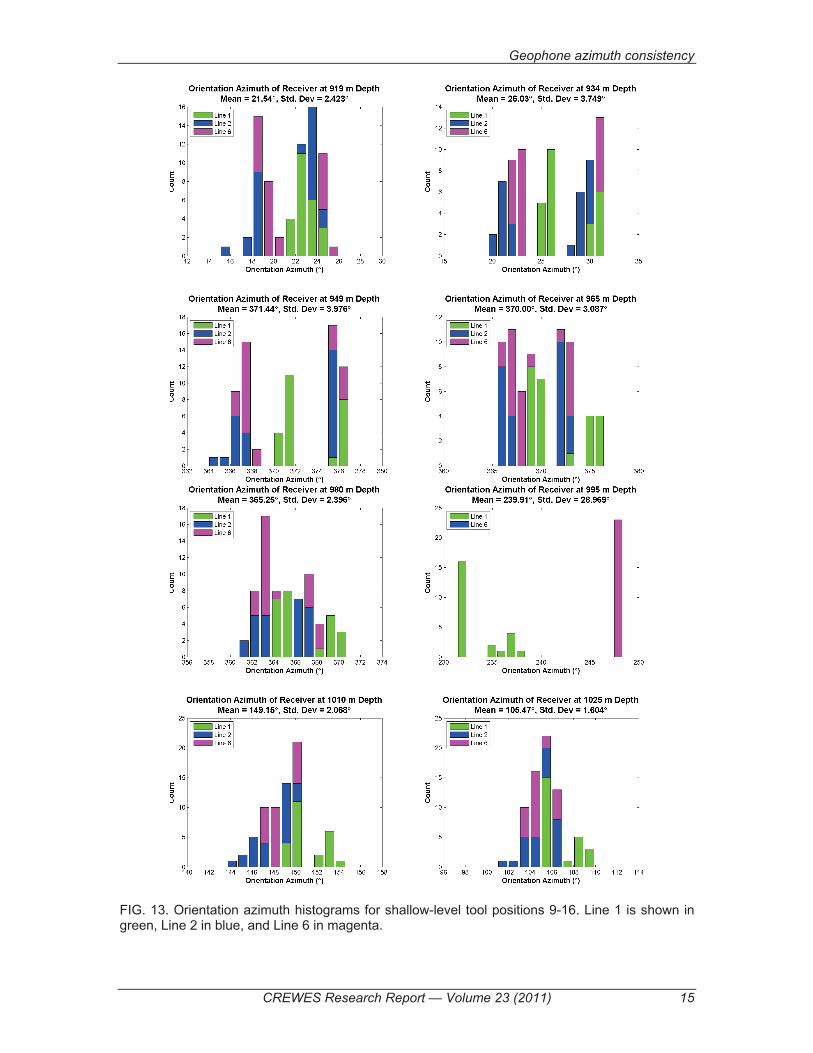
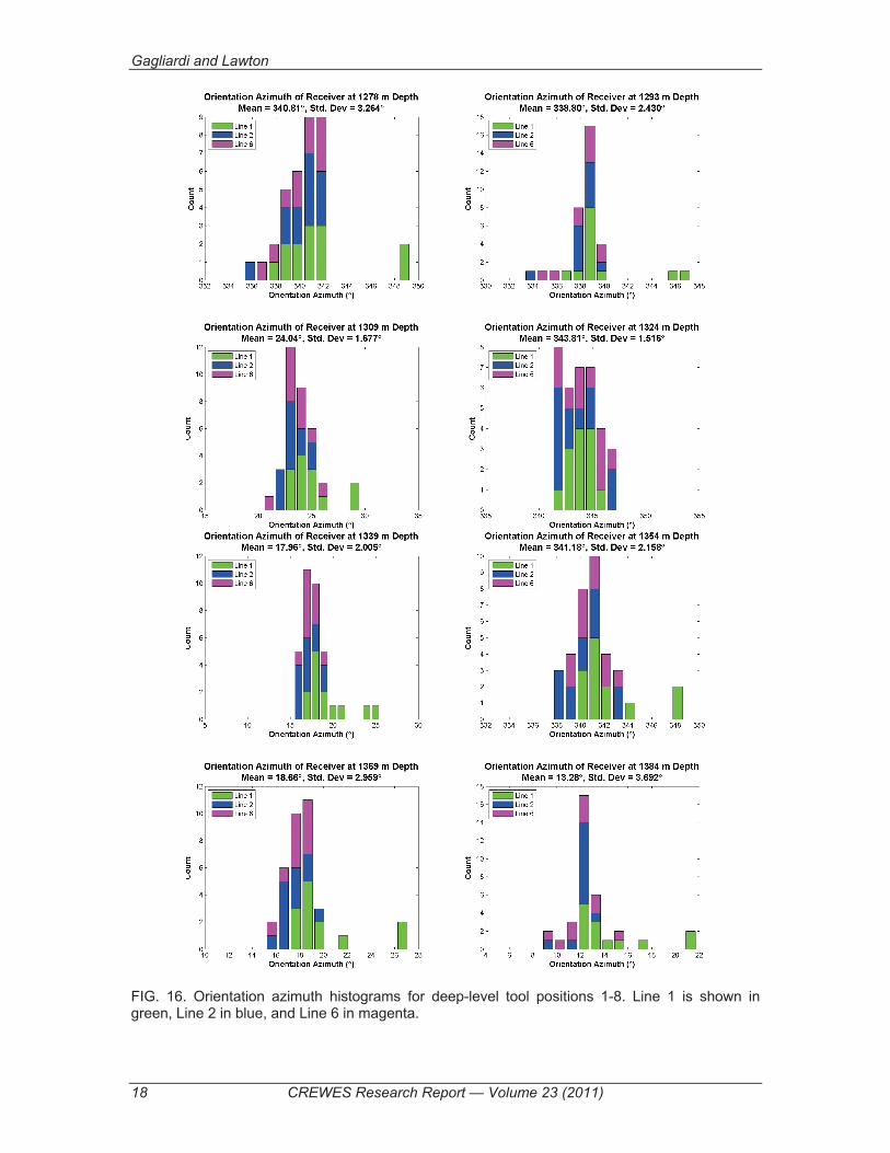
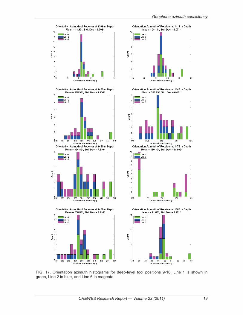
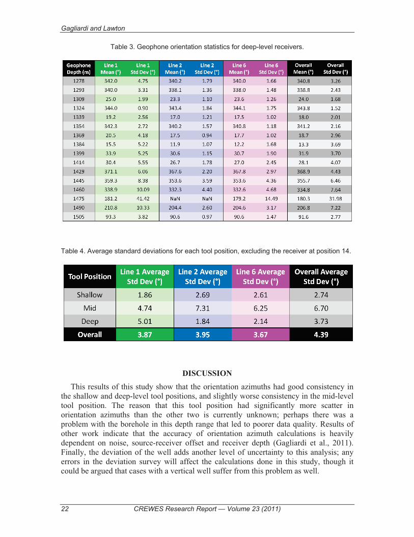
Statistical analysis of the calculated orientation azimuths confirms this distinction between lines. Histograms of these angles (Figures 12-17), along with numerical analysis of their means and standard deviations (Tables 1-3) clearly show that angle calculations using Line 1 consistently lead to larger values than calculations performed using either of Lines 2 or 6. On average, Line 1 calculated an angle 3.7° higher than Line 2 and 3.0° higher than Line 6. Figure 18 directly shows the differences in the mean orientation azimuths of each line. Finally, the average standard deviations for each line and tool position are shown in Table 4; the receiver at tool position 14 was not included in these calculations, as there were data quality problems with this receiver.

FIG. 5. Survey geometry of shots used in 16-level VSP experiment, after being projected using Equations 8 and 9. Shots are shown relative to the geophone location, displayed as a red square at the origin. Line 1 is shown in green, Line 2 is shown in blue and Line 6 is shown in magenta.



FIG. 6. Orientation azimuth vs. pseudo offset for shallow-level tool positions 1-8. Line 1 is shown in green, Line 2 in blue, and Line 6 in magenta.



FIG. 7. Orientation azimuth vs. pseudo offset for shallow-level tool positions 9-16. Line 1 is shown in green, Line 2 in blue, and Line 6 in magenta.



FIG. 8. Orientation azimuth vs. pseudo offset for mid-level tool positions 1-8. Line 1 is shown in green, Line 2 in blue, and Line 6 in magenta.



FIG. 9. Orientation azimuth vs. pseudo offset for mid-level tool positions 9-16. Line 1 is shown in green, Line 2 in blue, and Line 6 in magenta.



FIG. 10. Orientation azimuth vs. pseudo offset for deep-level tool positions 1-8. Line 1 is shown in green, Line 2 in blue, and Line 6 in magenta.



FIG. 11. Orientation azimuth vs. pseudo offset for deep-level tool positions 9-16. Line 1 is shown in green, Line 2 in blue, and Line 6 in magenta.



FIG. 12. Orientation azimuth histograms for shallow-level tool positions 1-8. Line 1 is shown in green, Line 2 in blue, and Line 6 in magenta.



FIG. 13. Orientation azimuth histograms for shallow-level tool positions 9-16. Line 1 is shown in green, Line 2 in blue, and Line 6 in magenta.



FIG. 14. Orientation azimuth histograms for mid-level tool positions 1-8. Line 1 is shown in green, Line 2 in blue, and Line 6 in magenta.



FIG. 15. Orientation azimuth histograms for mid-level tool positions 9-16. Line 1 is shown in green, Line 2 in blue, and Line 6 in magenta.



FIG. 16. Orientation azimuth histograms for deep-level tool positions 1-8. Line 1 is shown in green, Line 2 in blue, and Line 6 in magenta.



FIG. 17. Orientation azimuth histograms for deep-level tool positions 9-16. Line 1 is shown in green, Line 2 in blue, and Line 6 in magenta.



FIG. 18. Differences in mean orientation azimuth for each geophone depth. Differences between Line 1 and 2 are shown in black; differences between Line 1 and 6 are shown in red; and differences between Line 6 and 2 are shown in cyan.



Table 1. Geophone orientation statistics for shallow-level receivers.

Table 2. Geophone orientation statistics for mid-level receivers.



Table 3. Geophone orientation statistics for deep-level receivers.

Table 4. Average standard deviations for each tool position, excluding the receiver at position 14.

DISCUSSION This results of this study show that the orientation azimuths had good consistency in

the shallow and deep-level tool positions, and slightly worse consistency in the mid-level tool position. The reason that this tool position had significantly more scatter in orientation azimuths than the other two is currently unknown; perhaps there was a problem with the borehole in this depth range that led to poorer data quality. Results of other work indicate that the accuracy of orientation azimuth calculations is heavily dependent on noise, source-receiver offset and receiver depth (Gagliardi et al., 2011). Finally, the deviation of the well adds another level of uncertainty to this analysis; any errors in the deviation survey will affect the calculations done in this study, though it could be argued that cases with a vertical well suffer from this problem as well.



A previous study done in Violet Grove by Gagliardi and Lawton (2010), which used a geophone array that was cemented in place, showed slightly better consistency; Lines 1 and 2 were common to both of these studies. Standard deviation in geophone orientation azimuths was 3.9° overall, and 2.3° when only using source-well offsets greater than 500 m. However, the geophone array had been in place for 2 years, and three out of eight geophones had suffered damage to at least one component.

Perhaps the most interesting result seen in this study is the distinction in trends between the different source lines, particularly regarding Line 1, where the average separation of 3.7° from Line 2 and 3.0° from Line 6 could be a lithological indication rather than a statistical one; azimuthal anisotropy is a possible explanation, since there is a different directionality associated with each of the lines. Examination of the orientation azimuth vs. pseudo-offset plots provides even more compelling evidence that there are lithologic influences to this difference. The separation still falls within the standard deviation of all three lines overall, and statistically cannot confidently be deemed to show a significant difference; thus, a more detailed statistical analysis of these angles is warranted. Additionally, analysis of other field examples and synthetic models would provide some more insight.

CONCLUSIONS

� A method for examining borehole geophone orientation azimuths was successfully developed for the case of a deviated well.

� Orientation azimuths, using all three lines, had an average standard deviation of 4.39°.

� Orientation azimuth consistency was poorest for the mid-level tool position (6.70°), and best for the shallow-level tool position (2.74°).

� Orientation azimuth values calculated using sources from Line 1 were, on average, 3.7° higher than Line 2 and 3.0° higher than Line 6. This could be related to geological properties of the area, such as azimuthal anisotropy.

FUTURE WORK Firstly, modeling should be used to determine the possible effects of anisotropy on

borehole geophone orientation azimuth analysis. Other field studies should also be examined for similar effects; a 3D VSP survey would be particularly useful in this regard. If the results of this study are indeed indicative of anisotropy, it would suggest that further care is needed when analysing data from these geophones. It may also suggest that calibration of these geophones can provide us with useful information about anisotropy, which can then be used to improve geological models used in seismic imaging.



ACKNOWLEDGEMENTS We would like to thank Heather Lloyd and Chris Bird for valuable discussions and

encouragement in regards to the problems that arose with the well deviation. We would also like to thank GEDCO for the use of Vista software, and all CREWES sponsors.

REFERENCES Dashtgard, S. E., Buschkuehle, M. B. E., Berhane, M. and Fairgrieve, B., 2006, Local-Scale Baseline

Geological Report for the Pembina-Cardium CO2-Enhanced Oil Recovery Site: Alberta Geological Survey,

DiSiena, J. P., Gaiser, J. E. and Corrigan, D., 1984, Three-component vertical seismic profiles; orientation of horizontal components for shear wave analysis, in Toksoz, M. N. and Stewart, R. R., eds., Vertical seismic profiling, Part B Advanced concepts: , 189-204.

Gagliardi, P., 2011, Innanen, K. A. H. And Lawton, D. C., 2011, Effects of noise on geophone orientation azimuth determination: CREWES Research Report, 23 (this report).

Gagliardi, P. and Lawton, D. C., 2010, Borehole geophone repeatability experiment: CREWES Research Report, 22, 22.1-22.23.

Hitchon, B., 2009, Pembina Cardium CO2 Monitoring Pilot: A CO2

-EOR Project, Alberta, Canada: Final Report: Geoscience Publishing, Limited.

APPENDIX A: VECTOR BASIS OF DEVIATED WELL

In order to form a vector basis in 3-D, three vectors, ��, �� and � �, must be defined such that the following conditions are satisfied:

�� = 0; (A.1)

�� × �� = � �; (A.2)

and

||��|| = || ��|| = ||� �|| = 1. (A.3)

Additionally, �� and �� need to be defined on the plane defined by the normal ��, which implies

�� = �� = 0. (A.4)

Using �� and �� defined in (6) and (7), we can check condition (A.1):

�� = �� sin��cos��0 � � �� cos �� cos��cos �� sin��sin �� Calculating the dot product gives



= �(� sin��)(� cos ��) cos�� + (cos�� (� cos ��) sin��) + �0(sin ��)�

= sin�� cos�� cos �� sin�� cos�� cos �� + 0

= 0 .

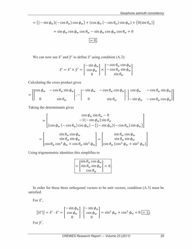
We can now use �� and �� to define � � using condition (A.2):

� � = �� × �� = �� sin��cos��0 � × �� cos �� cos�� cos �� sin��sin �� Calculating the cross product gives

= �!cos�� cos �� sin��0 sin �� ! , � !� sin�� cos �� cos��

0 sin �� ! , ! cos �� cos �� sin�� sin�� cos �� cos��

!� Taking the determinants gives

= " cos�� sin �� 0�1(� sin��) sin ��(cos�� (� cos ��) cos��) � �(� sin��)(� cos ��) sin��#

= " sin �� cos��sin �� sin��cos �� cos� �� + cos �� sin� ��# = " sin �� cos��sin �� sin��cos �� (cos� �� + sin� ��)#

Using trigonometric identities this simplifies to

= �sin �� cos��sin �� sin��cos �� = �� .

In order for these three orthogonal vectors to be unit vectors, condition (A.3) must be satisfied:

For ��, $|��|$ = �� = �� sin��cos��0 � � �� sin��cos��0 � = sin� �� + cos� �� + 0 = 1 ;

For ��,



$| ��|$ = �� cos �� cos�� cos �� sin��sin �� cos �� cos�� cos �� sin��sin �� = cos� �� cos� �� + cos� �� sin� �� + sin� ��

= cos� �� (cos� �� + sin� ��) + sin� ��

= cos� �� + sin� �� = 1 ;

For � �, $|� �|$ = �sin �� cos��sin �� sin��cos �� sin �� cos��sin �� sin��cos �� = sin� �� cos� �� + sin� �� sin� �� + cos� ��

= sin� �� (cos� �� + sin� ��) + cos� ��

= sin� �� + cos� �� = 1 .

Finally, since we have �� = � �, the cross product of condition (A.2) forces condition (A.4) to become true. Therefore, the definitions of ��, � and �� form a suitable vector basis for a 3-component geophone in a deviated well.

geophone azimuth consistency from calibrated vertical ... · geophone azimuth consistency ......

Documents