geophys. j. int.-2016-bodin-605-29

Geophysical Journal InternationalGeophys. J. Int. (2016) 206, 605–629 doi: 10.1093/gji/ggw124Advance Access publication 2016 April 4GJI Seismology

Imaging anisotropic layering with Bayesian inversionof multiple data types

T. Bodin,1,2 J. Leiva,1 B. Romanowicz,1,3,4 V. Maupin5 and H. Yuan6

1Berkeley Seismological Laboratory, 215 McCone Hall, UC Berkeley, Berkeley CA 94720-4760, USA. E-mail: [email protected] Lyon, Universite Lyon 1, Ens de Lyon, CNRS, UMR 5276 LGL-TPE, F-69622 Villeurbanne, France3Insitut de Physique du Globe de Paris (IPGP), 1 Rue Jussieu F-75005 Paris, France4College de France, 11 place Marcelin Berthelot, F-75231 Paris, France5Department of Geosciences, University of Oslo, P.O. Box 1047, Blindern, Oslo 0316, Norway6Department of Earth and Planetary Sciences, Macquarie University, New South Wales 2109, Australia

Accepted 2016 March 31. Received 2016 March 31; in original form 2015 September 1

S U M M A R YAzimuthal anisotropy is a powerful tool to reveal information about both the present structureand past evolution of the mantle. Anisotropic images of the upper mantle are usually obtainedby analysing various types of seismic observables, such as surface wave dispersion curvesor waveforms, SKS splitting data, or receiver functions. These different data types sampledifferent volumes of the earth, they are sensitive to different length scales, and hence areassociated with different levels of uncertainties. They are traditionally interpreted separately,and often result in incompatible models. We present a Bayesian inversion approach to jointlyinvert these different data types. Seismograms for SKS and P phases are directly inverted usinga cross-convolution approach, thus avoiding intermediate processing steps, such as numericaldeconvolution or computation of splitting parameters. Probabilistic 1-D profiles are obtainedwith a transdimensional Markov chain Monte Carlo scheme, in which the number of layers, aswell as the presence or absence of anisotropy in each layer, are treated as unknown parameters.In this way, seismic anisotropy is only introduced if required by the data. The algorithm isused to resolve both isotropic and anisotropic layering down to a depth of 350 km beneathtwo seismic stations in North America in two different tectonic settings: the stable Canadianshield (station FFC) and the tectonically active southern Basin and Range Province (stationTA-214A). In both cases, the lithosphere–asthenosphere boundary is clearly visible, andmarked by a change in direction of the fast axis of anisotropy. Our study confirms thatazimuthal anisotropy is a powerful tool for detecting layering in the upper mantle.

Key words: Inverse theory; Body waves; Surface waves and free oscillations; Seismicanisotropy; North America.

1 I N T RO D U C T I O N

Seismic anisotropy in the crust and upper mantle can be producedby multiple physical processes at different spatial scales. In themantle, plastic deformation of olivine aggregates results in a crys-tallographic preferential orientation (CPO) of minerals, and pro-duces large-scale seismic anisotropy that can be observed seismo-logically. These observations are usually related to the strain field,and interpreted in terms of either present day flow, or ‘frozen’ flowfrom the geological past. Furthermore, the spatial distribution ofcracks, fluid inclusions, or seismic discontinuities can induce appar-ent anisotropy, called shape-preferred orientation (SPO) anisotropy(Crampin & Booth 1985; Backus 1962). In this way, anisotropicproperties of rocks are closely related to their geological historyand present configuration, and hence reveal essential information

about the Earth’s structure and dynamics (e.g. Montagner & Guillot2002).

Observations of seismic anisotropy depend on the 21 parametersof the full elastic tensor. However, all these parameters cannot beresolved independently at every location, and seismologists usuallyrely on simplified assumptions on the type of anisotropy, namelyhexagonal symmetry. This type of anisotropy is defined by the fiveLove parameters of transverse isotropy (A, C, F, L, N) and two anglesdescribing the direction of the axis of symmetry (Love 1927). Mostseismological studies assume one of two types of anisotropy: (1)radial anisotropy, where the axis of hexagonal symmetry is verticaland with no azimuthal dependence and (2) azimuthal anisotropy,where the axis of hexagonal symmetry is horizontal with unknowndirection. Retrieving the tilt of the hexagonal axis of symmetry is inprinciple possible (Montagner & Nataf 1988; Plomerova & Babuska

C© The Authors 2016. Published by Oxford University Press on behalf of The Royal Astronomical Society. 605

by guest on September 6, 2016

http://gji.oxfordjournals.org/D

ownloaded from

mailto:[email protected]

http://gji.oxfordjournals.org/

606 T. Bodin et al.

2010; Xie et al. 2015), but in practice difficult, due to limitations inthe available azimuthal coverage, trade-offs with other competingfactors, such as tilted layers in the case of body waves and non-uniqueness of the solution in the case of surface waves inversion.

Azimuthal anisotropy in the crust and upper mantle can be ob-served from different seismic measurements, sampling the Earthat different scales: surface wave observations, core-refracted shearwave (SKS) splitting measurements and receiver functions. The lat-ter two methods rely on relatively high-frequency teleseismic bodywaves measurements, and therefore can provide good lateral resolu-tion in those areas of continents where broad-band station coverageis dense, if good azimuthal coverage is available.

Receiver functions have the potential of resolving layeredanisotropic structure locally. Large data sets from single seismicstations have been used to image both anisotropic and dipping struc-tures primarily at crustal depths (e.g. Kosarev et al. 1984; Levin &Park 1997; Peng & Humphreys 1997; Savage 1998; Farra & Vinnik2000; Frederiksen & Bostock 2000; Leidig & Zandt 2003; Vergneet al. 2003; Schulte-Pelkum & Mahan 2014; Audet 2015; Bianchiet al. 2015; Liu et al. 2015; Vinnik et al. 2016). Harmonic decompo-sition methods have been developed to distinguish the contributionsfrom isotropic and anisotropic discontinuities, and dipping layers(Kosarev et al. 1984; Girardin & Farra 1998; Bianchi et al. 2010).

Shear wave splitting measurements in core-refracted phases (SKSand SKKS) provide constraints on the integrated effect of azimuthalanisotropy across the thickness of the mantle beneath a single sta-tion (e.g. Vinnik et al. 1984, 1989; Silver & Chan 1991; Vinniket al. 1992; Silver 1996; Long & Silver 2009), but depth resolu-tion is generally poor, even when considering finite-frequency ker-nels (Chevrot 2006), and there are trade-offs between the strengthof anisotropy and the thickness of the anisotropic domain. Dueto the lack of sufficient azimuthal coverage to distinguish morethan one layer, shear wave splitting measurements are usually in-terpreted under the assumption of a single layer of anisotropy witha horizontal axis of symmetry. We note however several attemptsto map multiple layers as well as a dipping fast axis (Silver &Savage 1994; Levin et al. 1999; Hartog & Schwartz 2000; Yuanet al. 2008).

Surface wave tomographic inversions provide constraints onboth radial (Gung et al. 2003; Plomerova et al. 2002; Nettles &Dziewonski 2008; Fichtner et al. 2010) and azimuthal anisotropy atthe regional (Forsyth 1975; Simons et al. 2002; Deschamps et al.2008; Beghein et al. 2010; Fry et al. 2010; Adam & Lebedev 2012;Darbyshire et al. 2013; Zhu & Tromp 2013; Legendre et al. 2014;Kohler et al. 2015) and global scale (Tanimoto & Anderson 1985;Montagner & Nataf 1986; Trampert & van Heijst 2002; Trampert& Woodhouse 2003; Debayle et al. 2005; Beucler & Montagner2006; Visser et al. 2008; Debayle & Ricard 2012, 2013; Yuan &Beghein 2013, 2014). Surface waves provide better vertical resolu-tion than SKS data, but are limited in horizontal resolution due tothe long wavelengths. Still, the depth range where vertical resolu-tion is achieved depends on the frequency range considered (longerperiods sample deeper depths), as well as the type of surface wavesconsidered. Most studies are based on the analysis of fundamentalmode surface wave dispersion up to about 200–250 s, which havegood resolution down to lithospheric depths, although inclusion ofsurface wave overtones can improve resolution at depth (e.g. Yuan& Beghein 2014; Durand et al. 2015).

These three different data types are therefore characterized bydifferent sensitivities to structure. They are modelled with differentapproximations of the wave equation, and associated with differentnoise levels. A well-known problem is that they often provide incom-

patible anisotropic models, and lead to contradictory interpretations.For example, surface waves and SKS waves sample different vol-umes in the earth, and SKS splitting measurements often disagreewith predictions made from surface wave tomographic models (e.g.Montagner et al. 2000; Conrad et al. 2007; Becker et al. 2012; Wang& Tape 2014). This discrepancy can be explained by the progressiveloss of resolution of fundamental mode surface waves below depthsof 200–250 km. Furthermore, body waves and surface waves aremeasured in different frequency bands, and hence are sensitive tostructure at different wavelengths. The sharp discontinuities that canbe resolved by receiver functions are usually mapped into apparentradial anisotropy in smooth models constructed from surface waves(Capdeville et al. 2013; Bodin et al. 2015).

In order to improve resolution in anisotropy, several studies haveproposed joint inversion algorithms combining body waves and sur-face waves. Marone & Romanowicz (2007), Yuan & Romanowicz(2010b) and Yuan et al. (2011) iteratively combined 3-D waveformtomography (including fundamental surface waves and overtones)with constraints from shear wave splitting data in North Amer-ica. They showed that by incorporating body waves, the anisotropystrength significantly increases at the asthenospheric depth, whilethe directions remain largely unchanged. However, these modelsare obtained by linearized and damped inversions, where the pro-duced seismic models strongly depend on choices made at the out-set (reference model, regularization). This precludes propagationof uncertainties from observations to inverted models, and hencemakes the interpretation difficult. In another approach, Vinnik et al.(2007), Obrebski et al. (2010) and Vinnik et al. (2014) performeda 1-D Monte Carlo joint inversion of SKS and receiver functionsat individual broad-band stations, but long-wavelength informationfrom surface waves was not used in this case. Therefore, two mainchallenges remain in anisotropic imaging:

(i) To our knowledge, azimuthal variations of surface wave dis-persion measurements have never been inverted jointly with receiverfunctions.

(ii) It is difficult to jointly invert different data types, as invertedmodels strongly depend on the choice of parameters used to weighthe relative contribution of each data sets in the inversion.

In this work, we address these issues with a method for 1-D in-version under a seismic station. We jointly invert Rayleigh wavedispersion curves with their azimuthal variations, together withconverted body waves and SKS data. For body waves, standardinversion procedures are usually based on secondary observables,such as deconvolved waveforms (receiver functions) or splittingparameters for SKS data. Here, we directly invert the different com-ponents of seismograms with a cross-convolution approach, as thisallows us to better propagate uncertainties from recorded wave-forms towards a velocity model (Menke & Levin 2003; Bodin et al.2014). We cast the problem in a Bayesian framework, and explorethe space of earth models with a Markov chain Monte Carlo algo-rithm. This allows us to deal with the non-linear and non-uniquenature of the problem, and quantify uncertainties. The solution isa probabilistic 1-D profile describing shear wave velocity, strengthof azimuthal anisotropy and fast axis direction, at each depth. Weuse a transdimensional formulation where the number of layers aswell as the presence of anisotropy in each layer are treated as freevariables.



ownloaded from


Bayesian imaging of anisotropic layering 607

2 M E T H O D O L O G Y

2.1 Model parametrization

The full elastic tensor of 21 parameters is usually described withthe so-called Voigt notation 6 × 6 symmetric matrix Cmn (Maupin& Park 2007). An elastic medium with hexagonal (i.e. cylindrical)symmetry and horizontal axis of symmetry is called a horizontaltransverse isotropic model (HTI), and is usually defined by the fiveLove parameters of transverse isotropy A, C, F, L, N (Love 1927):

Cmn =

⎛⎜⎜⎜⎜⎜⎜⎜⎜⎜⎜⎝

A F (A − 2N ) 0 0 0

F C F 0 0 0

(A − 2N ) F A 0 0 0

0 0 0 L 0 0

0 0 0 0 N 0

0 0 0 0 0 L

⎞⎟⎟⎟⎟⎟⎟⎟⎟⎟⎟⎠

(1)

Here, axis 3 is vertical and axis 2 is the horizontal axis of symmetry.A, C, N and L can be related to P- and S-wave velocities in differentdirections. If ψ fast is the angle of the fast axis relative to North, thevelocity of S waves propagating horizontally and polarized vertically(SV waves) is given by (Crampin 1984):

ρV 2sv(ψ) = (L + N )

2+ (L − N )

2cos(2(ψ − ψfast)) (2)

where ψ is the direction of propagation relative to North. Thevelocity of P waves and SH waves propagating in the horizontalplane are a bit more complicated as they contain cos(4ψ) terms.The corresponding expressions can be found in Crampin (1984).

In this work, instead of using elastic parameters, we follow thenotation used in most body waves studies, and parametrize ourmodel in terms of seismic velocities, where the isotropic componentis given by the values of Vs and Vp, and the anisotropic component isdefined in terms of ‘peak to peak’ level of anisotropy δVp, δVs (e.g.Farra et al. 1991; Romanowicz & Yuan 2012). These parameters arerelated to the five elastic parameters A, C, F, L, N by the followingexpressions:

C

ρ=

(Vp + δVp

2

)2

,A

ρ=

(Vp − δVp

2

)2

, (3)

L

ρ=

(Vs + δVs

2

)2

,N

ρ=

(Vs − δVs

2

)2

, (4)

The elastic parameter F controls the velocity along the directionintermediate between the fast and the slow directions. It is com-mon to parametrize it with the fifth parameter η = F/(A − 2L),which we set to one (i.e. F = A − 2L) as in PREM (Dziewonski &Anderson 1981). Following Obrebski et al. (2010), we also imposeVp/VS = 1.7 for the sake of simplicity. The density ρ is calculatedthrough the empirical relation ρ = 2.35 + 0.036(Vp − 3)2 as done inTkalcic et al. (2006). In order to reduce the number of parameters,the ratio between the percentage of anisotropy for the compres-sional and shear waves (δVp/Vp)/(δVs/Vs) is fixed at 1.5 based onthe analysis of published data for the upper mantle (Obrebski et al.2010). Here, we acknowledge that surface waves and normal modesare sensitive to parameter η, Vp and density (Beghein & Trampert2004; Beghein et al. 2006; Kustowski et al. 2008), and that we couldhave easily treated these parameters as unknowns in the inversion.It has been demonstrated that η trade-offs with P-wave anisotropy(Beghein et al. 2006; Kustowski et al. 2008), implying that making

assumptions on either one of these parameters will likely affect re-sults and inferred model uncertainties. Although one could invertfor the entire elastic tensor in each layer, this would be at increasedcomputational cost. Here instead, we use these empirical scalingrelations to determine the least constrained parameters.

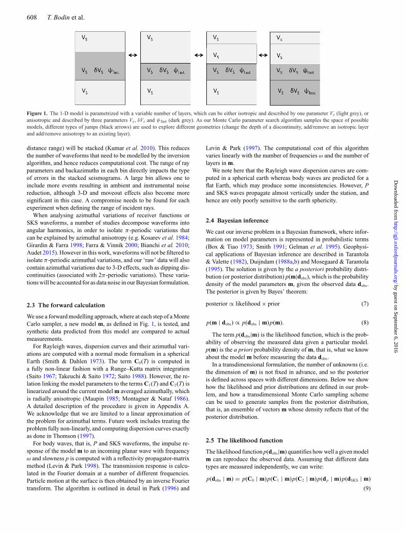
As shown in Fig. 1, our model is parametrized in terms of a stackof layers with constant seismic velocity. In our transdimensionalformalism, the number of unknowns is variable, as we want toexplain our data sets with the least number of free parameters. Eachlayer can be either isotropic and described solely by its shear wavevelocity Vs (in this case, δVs = 0), or azimuthally anisotropic anddescribed by three parameters: Vs, δVs and ψ fast the direction ofthe horizontal fast axis relative to the north. The layer thickness isalso variable and the last layer is a half-space. The other parameters(ρ, Vp, δVs) are given by the scaling relations mentioned above.

The number of layers k as well as the number of anisotropic layersl ≤ k are free parameters in the inversion (see Fig. 1). Therefore,the complete model to be inverted for is defined as

m = [z, Vs, δVs, � fast], (5)

where the vector z = [z1, . . . , zk] represents the depths of the k dis-continuities, Vs is a vector of size k and δVs, � fast are vectors of sizel. The total number of parameters in the problem (i.e. the dimensionof vector m) is therefore 2(k + l). We shall show how a Monte Carloalgorithm can explore different types of model parametrizations.

As in any data inference problem, it is clear that observations canalways be better explained with more model parameters (with l andk large). However, we will see that in a Bayesian framework, overlycomplex models with a large number of parameters have a lowerprobability and are naturally penalized. Between a simple and acomplex model that fit the data equally well, the simple one will bepreferred. With this formulation, anisotropy will only be includedinto the model if required by the data.

When inverting long-period seismic waves, this flexible approachto parametrizing an elastic medium allowed us to quantify the trade-off between vertical heterogeneities (lots of small isotropic layers)and radial anisotropy (fewer anisotropic layers) (Bodin et al. 2015).This trade-off can be broken by adding higher frequency observa-tions from body waves, thus allowing a consistent interpretation ofdifferent data types.

2.2 The data

For surface waves, we assume that some previous analysis (local ortomographic) provides us with the phase velocity dispersion at thestation and its azimuthal variation. To first order, the phase velocityof surface waves in an anisotropic medium can be written as:

C(T, ψ) = C0(T ) + C1(T ) cos(2ψ) + C2(T ) sin(2ψ)

+ C3(T ) cos(4ψ) + C4(T ) sin(4ψ) (6)

where T is the period and ψ is the direction of propagation relative tothe north (Smith & Dahlen 1973). For fundamental mode Rayleighwaves, the 2ψ terms C1 and C2 are sensitive to depth variationsof Vs, δVs and ψ fast, and the 4ψ terms are negligible, due to thelow amplitude of sensitivity kernels (Montagner & Tanimoto 1991;Maupin & Park 2007). We will therefore only invert C0(T), C1(T)and C2(T), and ignore 4ψ terms.

For body waves, recorded seismograms of P and SKS phasesfor events coming from different backazimuths will be inverted.To reduce the level of noise in P waveforms, individual eventscoming from the same regions (i.e. within a small backazimuth–



ownloaded from


608 T. Bodin et al.

Figure 1. The 1-D model is parametrized with a variable number of layers, which can be either isotropic and described by one parameter Vs (light grey), oranisotropic and described by three parameters Vs, δVs and ψ fast (dark grey). As our Monte Carlo parameter search algorithm samples the space of possiblemodels, different types of jumps (black arrows) are used to explore different geometries (change the depth of a discontinuity, add/remove an isotropic layerand add/remove anisotropy to an existing layer).

distance range) will be stacked (Kumar et al. 2010). This reducesthe number of waveforms that need to be modelled by the inversionalgorithm, and hence reduces computational cost. The range of rayparameters and backazimuths in each bin directly impacts the typeof errors in the stacked seismograms. A large bin allows one toinclude more events resulting in ambient and instrumental noisereduction, although 3-D and moveout effects also become moresignificant in this case. A compromise needs to be found for eachexperiment when defining the range of incident rays.

When analysing azimuthal variations of receiver functions orSKS waveforms, a number of studies decompose waveforms intoangular harmonics, in order to isolate π -periodic variations thatcan be explained by azimuthal anisotropy (e.g. Kosarev et al. 1984;Girardin & Farra 1998; Farra & Vinnik 2000; Bianchi et al. 2010;Audet 2015). However in this work, waveforms will not be filtered toisolate π -periodic azimuthal variations, and our ‘raw’ data will alsocontain azimuthal variations due to 3-D effects, such as dipping dis-continuities (associated with 2π -periodic variations). These varia-tions will be accounted for as data noise in our Bayesian formulation.

2.3 The forward calculation

We use a forward modelling approach, where at each step of a MonteCarlo sampler, a new model m, as defined in Fig. 1, is tested, andsynthetic data predicted from this model are compared to actualmeasurements.

For Rayleigh waves, dispersion curves and their azimuthal vari-ations are computed with a normal mode formalism in a sphericalEarth (Smith & Dahlen 1973). The term C0(T) is computed ina fully non-linear fashion with a Runge–Kutta matrix integration(Saito 1967; Takeuchi & Saito 1972; Saito 1988). However, the re-lation linking the model parameters to the terms C1(T) and C2(T) islinearized around the current model m averaged azimuthally, whichis radially anisotropic (Maupin 1985; Montagner & Nataf 1986).A detailed description of the procedure is given in Appendix A.We acknowledge that we are limited to a linear approximation ofthe problem for azimuthal terms. Future work includes treating theproblem fully non-linearly, and computing dispersion curves exactlyas done in Thomson (1997).

For body waves, that is, P and SKS waveforms, the impulse re-sponse of the model m to an incoming planar wave with frequencyω and slowness p is computed with a reflectivity propagator-matrixmethod (Levin & Park 1998). The transmission response is calcu-lated in the Fourier domain at a number of different frequencies.Particle motion at the surface is then obtained by an inverse Fouriertransform. The algorithm is outlined in detail in Park (1996) and

Levin & Park (1997). The computational cost of this algorithmvaries linearly with the number of frequencies ω and the number oflayers in m.

We note here that the Rayleigh wave dispersion curves are com-puted in a spherical earth whereas body waves are predicted for aflat Earth, which may produce some inconsistencies. However, Pand SKS waves propagate almost vertically under the station, andhence are only poorly sensitive to the earth sphericity.

2.4 Bayesian inference

We cast our inverse problem in a Bayesian framework, where infor-mation on model parameters is represented in probabilistic terms(Box & Tiao 1973; Smith 1991; Gelman et al. 1995). Geophysi-cal applications of Bayesian inference are described in Tarantola& Valette (1982), Duijndam (1988a,b) and Mosegaard & Tarantola(1995). The solution is given by the a posteriori probability distri-bution (or posterior distribution) p(m|dobs), which is the probabilitydensity of the model parameters m, given the observed data dobs.The posterior is given by Bayes’ theorem:

posterior ∝ likelihood × prior (7)

p(m | dobs) ∝ p(dobs | m)p(m). (8)

The term p(dobs|m) is the likelihood function, which is the prob-ability of observing the measured data given a particular model.p(m) is the a priori probability density of m, that is, what we knowabout the model m before measuring the data dobs.

In a transdimensional formulation, the number of unknowns (i.e.the dimension of m) is not fixed in advance, and so the posterioris defined across spaces with different dimensions. Below we showhow the likelihood and prior distributions are defined in our prob-lem, and how a transdimensional Monte Carlo sampling schemecan be used to generate samples from the posterior distribution,that is, an ensemble of vectors m whose density reflects that of theposterior distribution.

2.5 The likelihood function

The likelihood function p(dobs|m) quantifies how well a given modelm can reproduce the observed data. Assuming that different datatypes are measured independently, we can write:

p(dobs | m) = p(C0 | m)p(C1 | m)p(C2 | m)p(dp | m)p(dSKS | m)

(9)



ownloaded from



where C0, C1 and C2 are surface wave dispersion curves (see eq. 6),and where dP and dSKS are seismograms observed for P and SKSwaves.

2.5.1 Surface wave measurements

For Rayleigh wave dispersion curves (C0(T), C1(T) and C2(T)),we assume that data errors (both observational and theoretical)are not correlated and are distributed according to a multivariatenormal distribution with zero mean and variances σC0 , σC1 andσC2 respectively. For C0(T), the likelihood probability distributionwrites:

p(C0 | m) = 1

(√

2πσC0 )n× exp

{−‖C0 − c0(m)‖2

2σ 2C0

}, (10)

where n is the number of data points, that is, the number of periodsconsidered and c0(m) is the dispersion curve predicted for modelm. In the same way, we define the likelihoods for 2ψ terms p(C1|m)and p(C2|m).

2.5.2 A cross-convolution likelihood function for body waves

In traditional receiver function analysis, the vertical componentof a P waveform is deconvolved from the horizontal components,to remove source and distant path effects (Langston 1979). Theresulting receiver function waveform can then be inverted for a 1-Dseismic model, by minimizing the difference between observed andpredicted receiver functions:

φ(m) =∥∥∥∥Hobs(t)

Vobs(t)− h(t, m)

v(t, m)

∥∥∥∥, (11)

where Vobs(t) and Hobs(t) are observed seismograms for verticaland radial components, and v(t, m) and h(t, m) are the verticaland radial impulse response functions of the near receiver structure,calculated for model m. Here, the division sign represents a spectraldivision, or deconvolution. Although receiver function analysis hasbeen extensively used for years, there are two well-known issues:

(i) The deconvolution is a numerical unstable procedure thatneeds to be stabilized (e.g. water level deconvolution; use of alow-pass filter). This results in a loss of resolution, which trade-offswith errors in the receiver function.

(ii) Uncertainties in receiver functions are therefore difficult toestimate.

These two issues have been well studied in the last decades (e.g.Park & Levin 2000; Kolb & Lekic 2014). Following Menke & Levin(2003), we propose a misfit function for inverting converted bodywaves without deconvolution, by defining a vector of residuals asfollows (Bodin et al. 2014):

r(m, t) = v(t, m) ∗ Hobs(t) − h(t, m) ∗ Vobs(t), (12)

where the sign ∗ represents a time-domain discrete convolution.The vector r is a function of observed and predicted data definedsuch that the unknown source function and distant path effectsare accounted for in both terms giving r = 0 for the true modelparameters m and zero errors. The norm ‖r(m)‖ is used as a misfitfunction, and is equivalent to the distance between observed andpredicted receiver functions in (11). However, (1) it does not involveany deconvolution and no damping parameters need to be chosen;(2) the probability density function for r(m, t) can be estimated fromerrors statistics in observed seismograms. If we assume that errors

Table 1. Possible component pairs that can be used in an inversion basedon the cross-convolution misfit function defined by Menke & Levin (2003).These four different pairs have complementary sensitivities to seismic dis-continuities and anisotropy. The advantage of a cross-convolution misfitfunction is that these different data types can all be inverted in the samemanner.

Conversions PSV R-Z components Phase PConversions PSH T-Z components Phase PConversions SP R-Z components Phase SSKS splitting R-T components Phases SKS and SKKS

in Vobs(t) and Hobs(t) are normally distributed and not correlated(Gaussian white noise), we have (see Appendix B for details):

p(r | m) = 1

(√

2πσp)n× exp

{−‖r(m)‖2

2σ 2p

}. (13)

For a given P waveform dp = [Vobs(t), Hobs(t)], resulting from astack of events coming from similar distances and backazimuths,we use the distribution in (13) as the likelihood function p(dp|m) toquantify the level of agreement between observations and the pre-dictions from a proposed earth model. Then, we combine a numberof stacked waveforms measured at different backazimuths–distancebins by simply using the product of their likelihoods, thus resultingin a joint inversion of several waveforms with different incidenceangles. A clear advantage is that we can use the same formalismto construct the likelihood function for SKS waveforms p(dSKS|m),as the vertical and radial components need simply be replaced byradial and transverse. The cross-convolution misfit function canalso be used for incoming S waves, that is, SP receiver functions,or transverse receiver functions, where the vertical component of aP waveform is deconvolved from its transverse component (seeTable 1). In this way, we can integrate various data types in aconsistent manner, with different sensitivities to the isotropic andanisotropic seismic structure beneath a station.

However, we acknowledge here that p(r|m) is not exactly a like-lihood function per se, as it does not represent the probability dis-tribution of data vectors Vobs(t) and Hobs(t), but rather the distri-bution of a vector of residuals conveniently defined. In a Bayesianframework, the vector of residuals is usually defined as a differencebetween observed data and predicted data: r(m) = dobs − dest(m).In this case, the distribution of r for a given model m gives thedistribution of the observed data (p(r|m) = p(dobs|m)). Howeverhere, p(r|m) does not strictly represent the probability of observingthe data, and hence cannot be strictly interpreted as a likelihoodfunction. We note that this way of approximating the likelihood bythe distribution of some residuals is also used by Stahler & Sigloch(2014), who proposed a Bayesian moment tensor inversion basedon a cross-correlation misfit function. For a fully rigorous Bayesianapproach to inversion of converted body waves, we refer the readerto Dettmer et al. (2015), who treated the source time function as anunknown in the problem.

2.6 Hierachical Bayes

The level of data errors for different data sets (σC0 , σC1 , σC2 , σ p,σ SKS, etc.) determines the width of the different Gaussian likelihoodfunctions in (9), and hence the relative weight given to differentdata types in the inversion. Here, the level of noise also accountsfor theoretical errors, that is, the part of the signal that we are notable to explain with our simplified 1-D parametrization and forwardtheory (Gouveia & Scales 1998; Duputel et al. 2014). For example,surface waves are sensitive to a larger volume around the station,



ownloaded from


610 T. Bodin et al.

compared to higher frequency body waves arriving at the stationwith a near vertical incidence angle. Lateral inhomogeneities in theearth will then produce an incompatibility between these two typesof observations, which here will be treated as data uncertainty.

In this work, we use a Hierarchical Bayes approach, and treatnoise parameters as unknown in the inversion (Malinverno & Briggs2004; Malinverno & Parker 2006). That is, each noise parameter isgiven a uniform prior distribution, and different values of noise (i.e.different weights) will be explored in the Monte Carlo parametersearch. The range of possible noise parameters, that is, the width ofthe uniform prior distribution, is set large enough so that it does notaffect final results (Bodin et al. 2012b). We then avoid the choicefor arbitrary weights from the user, and the relative quantity ofinformation brought by different data types is directly constrainedby the data themselves.

2.7 The prior distribution

The Bayesian formulation enables one to account for prior knowl-edge, provided that this information can be expressed as a prob-ability distribution p(m) (Gouveia & Scales 1998). In a transdi-mensional case, the prior distribution prevents the algorithm fromadding too many layers, as it naturally penalizes models with a largenumber of parameters [l, k].

To illustrate this, let us look at the prior on the vector of isotropicvelocity parameters Vs = [v1, . . . , vk]. We consider the velocity ineach layer as a priori independent, that is, no smoothing constraintis applied, and then write:

p(Vs | k) =k∏

i=1

p(vi ). (14)

For each parameter vi, we use a uniform prior distribution over therange [Vmin Vmax]. This uniform distribution integrates to one, andhence p(vi) = 1/V, where V = (Vmax − Vmin). Therefore, for agiven number of layers k we can write the prior on the vector Vs

as:

p(Vs | k) =(

1

V

)k

. (15)

Here, the prior on velocity parameters decreases exponentially withk, and complex models with many layers are penalized. The com-plete mathematical form of our prior distribution including all modelparameters is detailed in Appendix C.

In this way, the prior and likelihood distributions in our problemare in competition as complex models providing a good data fit(high likelihood) are simultaneously penalized with a low priorprobability. This is an example of an implementation of the generalprinciple of parsimony (or Occam’s razor) that states that betweentwo models (or theories) that predict the data equally well, thesimplest should be preferred (see Malinverno 2002, for details).Although k is a free parameter that will be constrained by the data,the user still needs to choose the width of the prior distributionV, which directly determines the volume of the model space, andhence the relative balance between the prior and the likelihood. Thechoice of V therefore directly determines the number of layers inthe solution models.

As expected, there is also a trade-off between the complexityof the model and the inferred value of data errors (σC0 , σC1 , σC2 ,σ p, σ SKS, etc.). As the model complexity increases, the data can bebetter fit, and the inferred value of data errors decrease. However,this degree of trade-off is limited and the data clearly constrains the

joint distribution of different parameters reasonably well (see Bodinet al. 2012b, for details).

2.8 Transdimensional sampling

Given the Bayesian framework described above, our goal is to gen-erate a large number of 1-D profiles, the distribution of which ap-proximates the posterior function. In our problem, the posteriordistribution is defined in a space of variable dimension (i.e. transdi-mensional), and can be sampled with the reversible-jump Markovchain Monte Carlo (rj-McMC) sampler (Geyer & Møller 1994;Green 1995, 2003), which is a generalization of the well-knownMetropolis–Hastings algorithm (Metropolis et al. 1953; Hastings1970). A general review of transdimensional Markov chains is givenby Sisson (2005).

The first use of these algorithms in the Geosciences was by Ma-linverno (2002) in the inversion of DC resistivity sounding data toinfer 1-D depth profiles. Further applications of the rj-McMC haverecently appeared in a variety of geophysical and geochemical datainference problems, including regression analysis (Gallagher et al.2011; Bodin et al. 2012a; Choblet et al. 2014; Iaffaldano et al. 2014),geochemical mixing problems (Jasra et al. 2006), thermochronol-ogy (Stephenson et al. 2006; Fox et al. 2015b), geomorphology (Foxet al. 2015a), seismic tomography (Young et al. 2013a,b; Zulfakrizaet al. 2014; Pilia et al. 2015), inversion of receiver functions (Pi-ana Agostinetti & Malinverno 2010; Bodin et al. 2012b; Fontaineet al. 2015), geoacoustics (Dettmer et al. 2010, 2013; Dosso et al.2014) and exploration geophysics (Malinverno & Leaney 2005; Rayet al. 2014). For an overview of the general methodology and itsapplication to Earth Science problems, see also Sambridge et al.(2006), Gallagher et al. (2009) and Sambridge et al. (2013).

Here, we follow the implementation presented in Bodin et al.(2012b) for joint inversion of receiver functions and surface waves,but expand the parametrization to the case where a variable numberof unknown parameters is associated to each layer, that is, whereeach layer can be either isotropic or anisotropic. In this section, weonly briefly present the procedure, and give mathematical details ofour particular implementation in Appendices C–E.

The algorithm produces a sequence of models, where each is arandom perturbation of the last. The first sample is selected ran-domly (from the uniform distribution) and at each step, the pertur-bation is governed by the so-called proposal probability distributionwhich only depends on the current model. The procedure for a giveniteration can be described as follows:

(i) Randomly perturb the current model m, to produce a pro-posed model m′, according to some chosen proposal distributionq(m′|m) (e.g. add/remove a layer, add/remove anisotropy to an ex-isting layer, change the depth of a discontinuities, etc.). For details,see Appendix D.

(ii) Randomly accept or reject the proposed model (in terms ofreplacing the current model), according to the acceptance criterionratio α(m′|m). For details, see Appendix E.

Models generated by the chain are asymptotically distributed ac-cording to the posterior probability distribution (for a detailed proof,see Green 1995, 2003). If the algorithm is run long enough, thesesamples should then provide a good approximation of the poste-rior distribution for the model parameters, that is, p(m|dobs). Thisensemble solution contains many models with variable parametriza-tions, and inference can be carried out by plotting the histogram of



ownloaded from



Figure 2. Synthetic body waves for the model shown in black in Fig. 3. Left: three component waveforms for an incoming P wave. Right: three componentwaveforms for four incoming SV waves arriving at different backazimuths (10◦, 55◦, 100◦, 145◦).

the parameter values (e.g. velocity at a given depth) in the ensemblesolution.

3 S Y N T H E T I C T E S T S

We first test our algorithm on synthetic data, and design an Earthmodel consisting of eight layers, among which only three areanisotropic (black line in Fig. 3). We use a reflectivity scheme(Levin & Park 1998) to propagate an incoming P wave, as well asfour SV waves coming from different backazimuths (10◦, 55◦, 100◦,145◦). There is only one P waveform here, and hence anisotropywill be constrained only from S waves in this experiment. Syntheticwaveforms (Fig. 2) are created by convolving the Earth’s impulseresponse (a Dirac comb), with a smoothed box car function. Then,some random Gaussian white noise is added to the waveforms.We acknowledge that these synthetic seismograms are far from be-ing realistic, as for example observed S waves usually have a lowerfrequency content than P waveforms. The goal here is only to test theability of the inversion procedure to integrate different data types.We also generate synthetic Rayleigh wave dispersion curves C0(T),with 2ψ azimuthal terms C1(T) and C2(T), for periods between 20and 200 s, with added random noise (see Fig. 5).

The top panels of Fig. 3 show results when only Rayleigh wavedispersion measurements are inverted, that is, an ensemble of mod-els distributed according to p(m|C0, C1, C2). Surface waves arelong-period observations, and hence are only sensitive to the long-wavelength structure of the Earth. The sharp seismic discontinuitiespresent in the true model (in black in Fig. 3A) cannot be resolved,and as expected, only a smooth averaged structure is recovered. Inour method, there is no need for statistical tests or regularizationprocedures to choose the adequate model complexity or smooth-ness corresponding to a given degree of data uncertainty. Instead,the reversible jump technique automatically adjusts the underlyingparametrization of the model to produce solutions with appropriatelevel of complexity to fit the data to statistically meaningful levels.This probabilistic scheme therefore allows us to quantify uncer-

tainties in the solution, and level of constraints. For example, weobserve that the direction of anisotropy in Fig. 3C is clearly betterresolved than its amplitude in Fig. 3B.

Bottom panels of Fig. 3 show results for a joint inversion of sur-face waves and body waves. For body waves, we jointly invert fourdata types: PSV, PSH, SP and SKS waveforms, given by all pairs ofcomponents described in Table 1. Here, both discontinuities andamplitude of anisotropy are better resolved, due to the complemen-tary information brought by body waves, although we acknowledgethat the distribution for the direction of anisotropy becomes bimodalbelow 250 km, certainly due to the lack of resolution at these depths.

Our Monte Carlo sampling of the model space allows us to treatthe problem in a fully non-linear fashion (although we acknowledgethat the function linking the model to C1(T), and C1(T) has beenlinearized around the isotropic average of the model). Contrary tolinear or linearized inversions, here the solution is not simply de-scribed by a Gaussian posterior probability function, and can bemultimodal. We illustrate this in Fig. 4 by showing the full distribu-tion for Vs, δVs and � fast at 150 km depth. The posterior distributionis shown in grey and the true model in red. This shows how addingbody waves reduces the width of the posterior distribution as moreinformation is added. Note that the distribution of the direction ofanisotropy is multimodal, with two secondary peaks correspondingto directions of other anisotropic layers in the model (green andblue lines). We acknowledge that a multimodal distribution is hardto interpret, as in this case the mean and standard deviation of thedistribution are meaningless.

Since the misfit function in eq. (12) is not a simple differencebetween observed and estimated data, it is difficult to get a visualidea of the level of data fit. Instead, in Fig. 5 we show the two termsof the misfit function, that is, vp(t, m)∗H(t) and hp(t, m)∗V(t) for thebest-fitting model m in the ensemble solution. Although these twowaveforms do not have any intuitive physical meaning, the misfitfunction has a minimum when these two vectors are equal, andplotting them together helps give a visual impression for the levelof fit. Right-hand panels of Fig. 5 show observed and best-fittingdata for surface wave observations C0(T), C1(T) and C2(T).



ownloaded from


612 T. Bodin et al.

Inc

Figure 3. Transdimensional inversion of synthetic data shown in Fig. 2. Density plots show the probability of the model given the data for our three unknownparameters: Vs (left), δVs (middle) and �fast (right). Black lines show the true model used to create noisy synthetic data. Top: inversion of surface wavedispersion only. Bottom: joint inversion of surface waves and body waves (i.e. PSV, PSH, SP and SKS waveforms).

4 A P P L I C AT I O N T O T W O D I F F E R E N TT E C T O N I C R E G I O N S I N N O RT HA M E R I C A

We apply this method to seismic observations recorded at two dif-ferent locations in North America. First, we invert data from stationFFC (Canada), which is a permanent, reliable and well-studied sta-tion located at the core of the Slave Craton. Since a large number ofstudies have already been published about the structure under thisstation (e.g. Ramesh et al. 2002; Rychert & Shearer 2009; Miller& Eaton 2010; Yuan & Romanowicz 2010b), we view this as anopportunity to test and validate the proposed scheme.

In a second step, we invert seismic data recorded in Arizona atstation TA-214A, of the US transportable array, which is a muchnoisier, recent, and less studied station, located in the southern Basinand Range Province, close to a diffuse plate boundary, where we

expect more complex 3-D structure due to recent tectonic activity.Here, 3-D effects in our data would not be able to be accountedfor by our 1-D model, and hence will be treated as data errors byour Bayesian scheme. The goal is to see how our inversion per-forms in a more difficult setting. The final results are summarizedin Fig. 11, where velocity gradients observed under the two sta-tions are interpreted in terms of well-known upper-mantle seismicdiscontinuities.

4.1 The North American craton

4.1.1 Tectonic setting

The North American craton comprises the stable portion of thecontinent, and differs from the more tectonically active Basin and



ownloaded from



Figure 4. Synthetic test. Posterior marginal distribution for Vs (left), δVs (middle) and �fast (right) at 150 km depth. Those are simply cross-sections of thedensity plots showed in Fig. 3. Red lines show the true model. In panels C and F, green and blue lines show the direction of anisotropy for the first and thirdlayer in the true model.

Figure 5. Synthetic data experiment. (a) Fit obtained by the cross-convolution modelling for the best-fitting model in the ensemble solution. (b) Fit to Rayleighwave dispersion data for the best-fitting model.

Range province to the west. In general, cratonic regions representareas of long-lived stability within the lithosphere that have re-mained compositionally unchanged, and have resisted destructionthrough subduction since as early as the Archean. Previous work inthis region reveals anomalously high seismic velocities in the uppermantle. Numerous seismic tomography studies detect the base ofthe lithosphere at a depth between 150 and 300 km throughout thestable craton (e.g. Gung et al. 2003; Kustowski et al. 2008; Net-tles & Dziewonski 2008; Romanowicz 2009; Ritsema et al. 2011;Pasyanos et al. 2014; Schaeffer & Lebedev 2014), but most receiverfunction studies fail to detect a corresponding drop in velocity atthis depth.

Receiver functions studies do show, however, a decrease in ve-locity within the cratonic lithosphere, suggesting the potential exis-tence of an intralithospheric discontinuity in this region (Abt et al.2010; Miller & Eaton 2010; Kind et al. 2012; Hansen et al. 2015;Hopper & Fischer 2015). For recent reviews on studies of the mid-

lithospheric discontinuity (MLD), see Rader et al. (2015), Karatoet al. (2015) and Selway et al. (2015). Evidence for anisotropiclayering within the cratonic lithosphere has also been previouslyshown (Yuan & Romanowicz 2010b; Wirth & Long 2014; Longet al. 2016).

The exact nature of the layered structure and composition of cra-tons, however, remains poorly understood. Competing hypothesesbased on geochemical and petrologic constraints describe possiblemodels for craton formation; these include underplating by hot man-tle plumes and accretion by shallow subduction zones in continentalor arc settings (Arndt et al. 2009).

4.1.2 The data

For Ps converted waveforms, we selected two regions with highseismicity (Aleutian islands and Guatemala) each defined by asmall backazimuth and distance range (Fig. 6). For both regions, we



ownloaded from


614 T. Bodin et al.

Figure 6. Body wave observations made at station FFC, Canada. For P waves, vertical and horizontal components are stacked over a set of events, at twodifferent locations (blue and green). For SKS data, the waveform of 12 individual events are used (red). SKS waveforms are normalized to unit energy, andthere is no amplitude information in the lower right-hand panel.



ownloaded from



computed stacks of seismograms following the approach of Kumaret al. (2010) and described in Bodin et al. (2014). Waveforms of firstP arrival are normalized to unit energy, aligned to maximum am-plitude, and sign reversal is applied when the P arrival amplitude isnegative. Moveout corrections are not needed here as stacked eventshave similar ray parameters. Both regions provide a pair of Vobs andHobs stacked waveforms. Since we only use two backazimuths, re-ceiver functions will not bring a lot of information about azimuthalanisotropy, which rather will be constrained from Rayleigh wavesand SKS waveforms.

For shear wave splitting measurements, a number of individualSKS waveforms have been selected at different backazimuths (redcircles in Fig. 6). The waveforms were manually picked based onsmall signal–noise ratio and large energy split onto the transversecomponent.

We also used fundamental mode Rayleigh wave phase velocitymeasurements (25–150 s) given by Ekstrom (2011) at this location.We recognize that these measurements are the result of a globaltomographic inversion, and hence are not free from artefacts dueto regularization and linearization. Better measurements could beobtained from local records obtained at small aperture arrays (e.g.Pedersen et al. 2006).

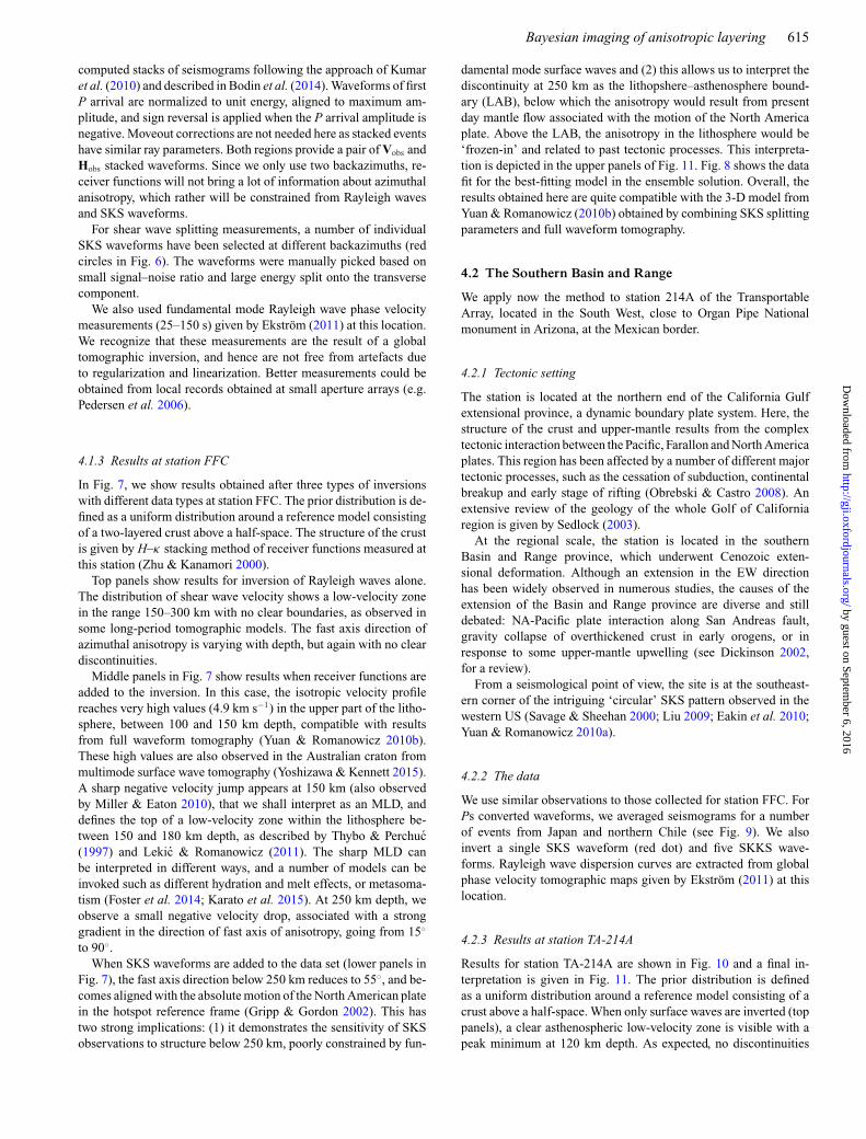
4.1.3 Results at station FFC

In Fig. 7, we show results obtained after three types of inversionswith different data types at station FFC. The prior distribution is de-fined as a uniform distribution around a reference model consistingof a two-layered crust above a half-space. The structure of the crustis given by H–κ stacking method of receiver functions measured atthis station (Zhu & Kanamori 2000).

Top panels show results for inversion of Rayleigh waves alone.The distribution of shear wave velocity shows a low-velocity zonein the range 150–300 km with no clear boundaries, as observed insome long-period tomographic models. The fast axis direction ofazimuthal anisotropy is varying with depth, but again with no cleardiscontinuities.

Middle panels in Fig. 7 show results when receiver functions areadded to the inversion. In this case, the isotropic velocity profilereaches very high values (4.9 km s−1) in the upper part of the litho-sphere, between 100 and 150 km depth, compatible with resultsfrom full waveform tomography (Yuan & Romanowicz 2010b).These high values are also observed in the Australian craton frommultimode surface wave tomography (Yoshizawa & Kennett 2015).A sharp negative velocity jump appears at 150 km (also observedby Miller & Eaton 2010), that we shall interpret as an MLD, anddefines the top of a low-velocity zone within the lithosphere be-tween 150 and 180 km depth, as described by Thybo & Perchuc(1997) and Lekic & Romanowicz (2011). The sharp MLD canbe interpreted in different ways, and a number of models can beinvoked such as different hydration and melt effects, or metasoma-tism (Foster et al. 2014; Karato et al. 2015). At 250 km depth, weobserve a small negative velocity drop, associated with a stronggradient in the direction of fast axis of anisotropy, going from 15◦

to 90◦.When SKS waveforms are added to the data set (lower panels in

Fig. 7), the fast axis direction below 250 km reduces to 55◦, and be-comes aligned with the absolute motion of the North American platein the hotspot reference frame (Gripp & Gordon 2002). This hastwo strong implications: (1) it demonstrates the sensitivity of SKSobservations to structure below 250 km, poorly constrained by fun-

damental mode surface waves and (2) this allows us to interpret thediscontinuity at 250 km as the lithopshere–asthenosphere bound-ary (LAB), below which the anisotropy would result from presentday mantle flow associated with the motion of the North Americaplate. Above the LAB, the anisotropy in the lithosphere would be‘frozen-in’ and related to past tectonic processes. This interpreta-tion is depicted in the upper panels of Fig. 11. Fig. 8 shows the datafit for the best-fitting model in the ensemble solution. Overall, theresults obtained here are quite compatible with the 3-D model fromYuan & Romanowicz (2010b) obtained by combining SKS splittingparameters and full waveform tomography.

4.2 The Southern Basin and Range

We apply now the method to station 214A of the TransportableArray, located in the South West, close to Organ Pipe Nationalmonument in Arizona, at the Mexican border.

4.2.1 Tectonic setting

The station is located at the northern end of the California Gulfextensional province, a dynamic boundary plate system. Here, thestructure of the crust and upper-mantle results from the complextectonic interaction between the Pacific, Farallon and North Americaplates. This region has been affected by a number of different majortectonic processes, such as the cessation of subduction, continentalbreakup and early stage of rifting (Obrebski & Castro 2008). Anextensive review of the geology of the whole Golf of Californiaregion is given by Sedlock (2003).

At the regional scale, the station is located in the southernBasin and Range province, which underwent Cenozoic exten-sional deformation. Although an extension in the EW directionhas been widely observed in numerous studies, the causes of theextension of the Basin and Range province are diverse and stilldebated: NA-Pacific plate interaction along San Andreas fault,gravity collapse of overthickened crust in early orogens, or inresponse to some upper-mantle upwelling (see Dickinson 2002,for a review).

From a seismological point of view, the site is at the southeast-ern corner of the intriguing ‘circular’ SKS pattern observed in thewestern US (Savage & Sheehan 2000; Liu 2009; Eakin et al. 2010;Yuan & Romanowicz 2010a).

4.2.2 The data

We use similar observations to those collected for station FFC. ForPs converted waveforms, we averaged seismograms for a numberof events from Japan and northern Chile (see Fig. 9). We alsoinvert a single SKS waveform (red dot) and five SKKS wave-forms. Rayleigh wave dispersion curves are extracted from globalphase velocity tomographic maps given by Ekstrom (2011) at thislocation.

4.2.3 Results at station TA-214A

Results for station TA-214A are shown in Fig. 10 and a final in-terpretation is given in Fig. 11. The prior distribution is definedas a uniform distribution around a reference model consisting of acrust above a half-space. When only surface waves are inverted (toppanels), a clear asthenospheric low-velocity zone is visible with apeak minimum at 120 km depth. As expected, no discontinuities



ownloaded from


616 T. Bodin et al.

Figure 7. Inversion results at station FFC, located in the North American Craton. Density plots represent the ensemble of models sampled by the reversiblejump algorithm, and represent the posterior probability function. The number of layers in individual models was allowed to vary between 2 and 60. For lowerplots, the maximum of the posterior distribution on the number of layers is 41.



ownloaded from



Figure 8. Station FFC (Canada). Data fit for best-fitting model collected by the Monte Carlo sampler. For body waves (left-hand panels), the cross-convolutionmisfit function is not constructed as a difference between observed and estimated data. Instead, we plot the two vectors H∗v(m) and V∗h(m), which differencewe try to minimize.

in the upper mantle are visible, due to the lack of resolution ofsurface waves. Middle panels in Fig. 10 are obtained after addingconverted P waves as constraints. As previously, seismic disconti-nuities are introduced. The bottom panels show results with SKSdata, providing deeper constrains on anisotropy, below 200 km.Fig. 12 shows the data fit for the best-fitting model in the ensemblesolution.

A clear negative discontinuity in Vs is visible at 100 km depthwith a positive jump at 150 km, thus producing a 50 km thick low-velocity zone that could be interpreted as the asthenosphere. In thiscase, the shallow LAB at 100 km is compatible with a number of SP

receiver functions studies in the region (Levander & Miller 2012;Lekic & Fischer 2014). This low-velocity zone lying under a highervelocity 100 km thick lithospheric lid has been also observed in theshear wave tomographic model of Obrebski et al. (2011). Here, thesharp LAB discontinuity cannot be solely explained by a thermalgradient, and hence suggests the presence of partial melt in the

asthenosphere in this region as proposed by Gao et al. (2004),Schmandt & Humphreys (2010) and Rau & Forsyth (2011).

The vertical distribution of fast axis direction (lower right-handpanel in Fig. 10) clearly shows three distinct domains:

(i) The lithospheric extension of the Basin and Range in theeast–west direction (90◦) is visible in the first 100 km. This direc-tion of anisotropy in this depth range is also observed in surfacewave (Zhang et al. 2007) or full waveform (Yuan et al. 2011) to-mographic models. This E-W direction of fast axis is close to beingperpendicular to the North America–Pacific plate boundary, andcorresponds to the direction of opening of the Gulf of Califor-nia; it is also similar to the direction of past subduction (Obrebskiet al. 2006). We also note that the direction of fast axis in the litho-sphere is gradually shifting to the North America absolute plate mo-tion direction when approaching 100 km depth (75◦ in the hotspotframe).



ownloaded from


618 T. Bodin et al.

Figure 9. Body wave observations used for the 1-D inversion under station 214A, located in the Basin and Range province. We use two stacks of P waveseismograms, from Japan (blue) and North Chile (green), as well as five SKKS individual waveforms (black) and one SKS waveform (red). SKKS and SKSwaveforms are normalized to unit energy, and there is no amplitude information in the lower right-hand panel.

(ii) There is a sharp change of direction of anisotropy at 100 kmdepth, which confirms the interpretation of the negative discontinu-ity as the LAB. A distinct layer between 100 and 180 km is clearlyvisible with a direction of 150◦, that is, parallel to the absoluteplate motion of the Pacific Plate, and in agreement with tomo-graphic inversions combining surface waveforms and SKS splittingdata (Yuan & Romanowicz 2010b). Also in agreement with thelatter study, anisotropy strength decreases beneath 200 km depth.

This direction is also compatible with shear wave splitting observa-tions obtained in the Mexican side of the southern Basin and Rangeprovince (Obrebski et al. 2006). Interestingly, this Pacific APM par-allel direction continues down to 180–200 km, that is, a bit belowthe bottom of the low-velocity zone as defined from the isotropicplot.

(iii) The jump at 180–200 km in the direction of anisotropy toabout 60◦ is a very interesting feature which seems associated with



ownloaded from



Figure 10. Inversion results at station TA-214A, located in the southern Basin and Range Province. Density plots represent the ensemble of models sampledby the reversible jump algorithm, and represent the posterior probability function. The number of layers in individual models was allowed to vary between 2and 80. For lower plots, the maximum of the posterior distribution on the number of layers is 55.

a positive step in the velocity, and could be the ‘Lehmann’ disconti-nuity (Gung et al. 2003). In that case, either Lehmann is not the baseof the asthenosphere, or the asthenosphere extends to ∼ 200 km, butconsists of two levels. The 60◦ direction between 200 and 350 kmmight reflect some secondary scale convection/dynamics in thisdepth range. However, the anisotropy signal is much weaker, or

more diffuse below 200 km, and one should not over interpret re-sults at these depths.

As expected, here the structure is clearly less well resolved thanfor station FFC, and in particular the amplitude and direction ofanisotropy below 200 km. This may be due to higher noise levels at



ownloaded from


620 T. Bodin et al.

Figure 11. Interpretation of results for both stations. Top: results at FFC (North American Craton) for joint inversion of surface waves, P and SKS waveforms.Bottom: results at TA-214A for joint inversion of surface waves, P and SKS waveforms. Vertical black lines represent the direction of the absolute motion ofthe North American plate in the hotspot reference frame (Gripp & Gordon 2002).

this temporary station, or because the structure is more complex andthe 1-D assumption less appropriate. In a complex 3-D setting, thefact that the data see different volumes results in incompatibilities,and here in wider posterior distributions.

5 C O N C LU S I O N S

We have presented a 1-D Bayesian Monte Carlo approach to con-strain depth variations in azimuthal anisotropy, by simultaneouslyinverting body and Rayleigh wave phase velocity measurementsobserved at individual stations. We use a flexible parametrizationwhere the number of layers, as well as the presence or absence of

anisotropy in each layer, are treated as unknown parameters, andare directly constrained by the data. This adaptive parametrizationturns out to be particularly useful, as the different types of datainvolved are sensitive to different volumes and length scales in theEarth. The level of noise in each data type (i.e. the required levelof fit) is also treated as an unknown to be inferred by the data. Inthis manner, both observational and theoretical data errors (effectof 3-D structure and dipping layers) are accounted for in the in-version, without need to choose weights to balance different datasets.

For the first time, azimuthal variations of dispersion curves werejointly inverted with receiver functions and SKS data, for bothcrust and upper-mantle structure. The procedure was applied to



ownloaded from



Figure 12. Station TA-214A (Arizona). Data fit for best-fitting model collected by the Monte Carlo sampler. For body waves (left-hand panels), the cross-convolution misfit function is not constructed as a difference between observed and estimated data. Instead, we plot the two vectors H∗v(m) and V∗h(m), thedifference between which we try to minimize.

data recorded at two different stations in North America, in twodifferent tectonic regimes. In both cases, results are compatible withprevious studies, and allow us to better image anisotropic layering.In both cases, we observed a LAB characterized by both isotropicand anisotropic sharp discontinuities in the mantle, thus implyingthat the LAB cannot be defined as a simple thermal transition, butalso reflects changes in composition and rheology.

A C K N OW L E D G E M E N T S

TB wishes to acknowledge support from the Miller Institute forBasic Research at the University of California, Berkeley. This workwas partially supported by a Labfees research collaborative grantfrom the U.C.O.P. (12-LR-236345) and by NSF Earthscope grantEAR-1460205.

R E F E R E N C E S

Abt, D.L., Fischer, K.M., French, S.W., Ford, H.A., Yuan, H. & Romanow-icz, B., 2010. North American lithospheric discontinuity structure im-aged by Ps and Sp receiver functions, J. geophys. Res., 115, B09301,doi:10.1029/2009JB006914.

Adam, J.M.-C. & Lebedev, S., 2012. Azimuthal anisotropy beneath South-ern Africa from very broad-band surface-wave dispersion measurements,Geophys. J. Int., 191(1), 155–174.

Arndt, N., Coltice, N., Helmstaedt, H. & Gregoire, M., 2009. Originof archean subcontinental lithospheric mantle: some petrological con-straints, Lithos, 109(1), 61–71.

Audet, P., 2015. Layered crustal anisotropy around the San Andreas Faultnear Parkfield, California: crustal anisotropy around San Andreas, J. geo-phys. Res., 120, 3527–3543.

Backus, G.E., 1962. Long-wave elastic anisotropy produced by horizontallayering, J. geophys. Res., 67(11), 4427–4440.

Becker, T.W., Lebedev, S. & Long, M.D., 2012. On the relationship betweenazimuthal anisotropy from shear wave splitting and surface wave tomog-raphy, J. geophys. Res., 117(B1), B01306, doi:10.1029/2011JB008705.



ownloaded from


622 T. Bodin et al.

Beghein, C. & Trampert, J., 2004. Probability density functions for radialanisotropy: implications for the upper 1200 km of the mantle, Earthplanet. Sci. Lett., 217(1), 151–162.

Beghein, C., Trampert, J. & van Heijst, H.J., 2006. Radial anisotropyin seismic reference models of the mantle, J. geophys. Res.,111, B02303, doi:10.1029/2005JB003728.

Beghein, C., Snoke, J.A. & Fouch, M.J., 2010. Depth constraints on az-imuthal anisotropy in the Great Basin from Rayleigh-wave phase velocitymaps, Earth planet. Sci. Lett., 289(3), 467–478.

Beucler, E. & Montagner, J.-P., 2006. Computation of largeanisotropic seismic heterogeneities (CLASH), Geophys. J. Int., 165(2),447–468.

Bianchi, I., Park, J., Agostinetti, N.P. & Levin, V., 2010. Mapping seismicanisotropy using harmonic decomposition of receiver functions: an appli-cation to Northern Apennines, Italy, J. geophys. Res., 115(B12), B12317,doi:10.1029/2009JB007061.

Bianchi, I., Bokelmann, G. & Shiomi, K., 2015. Crustal anisotropy acrossnorthern Japan from receiver functions, J. geophys. Res., 120(7), 4998–5012.

Bodin, T. & Sambridge, M., 2009. Seismic tomography with the reversiblejump algorithm, Geophys. J. Int., 178(3), 1411–1436.

Bodin, T., Salmon, M., Kennett, B.L.N. & Sambridge, M., 2012a. Prob-abilistic surface reconstruction from multiple data sets: an examplefor the Australian Moho, J. geophys. Res., 117(B10), B10307, doi:10.1029/2012JB009547.

Bodin, T., Sambridge, M., Tkalcic, H., Arroucau, P., Gallagher, K. &Rawlinson, N., 2012b. Transdimensional inversion of receiver func-tions and surface wave dispersion, J. geophys. Res., 117, B02301,doi:10.1029/2011JB008560.

Bodin, T., Yuan, H. & Romanowicz, B., 2014. Inversion of receiver functionswithout deconvolution—application to the Indian craton, Geophys. J. Int.,196(2), 1025–1033.

Bodin, T., Capdeville, Y., Romanowicz, B. & Montagner, J.-P., 2015. In-terpreting radial anisotropy in global and regional tomographic models,in The Earth’s Heterogeneous Mantle, pp. 105–144, eds Khan, A. &Deschamps, F., Springer.

Box, G.E. & Tiao, G.C., 1973. Bayesian Inference in Statistical Inference,Addison-Wesley.

Capdeville, Y., Stutzmann, E., Wang, N. & Montagner, J.-P., 2013. Resid-ual homogenization for seismic forward and inverse problems in layeredmedia, Geophys. J. Int., 194(1), 470–487.

Chevrot, S., 2006. Finite-frequency vectorial tomography: a new methodfor high-resolution imaging of upper mantle anisotropy, Geophys. J. Int.,165(2), 641–657.

Choblet, G., Husson, L. & Bodin, T., 2014. Probabilistic surface reconstruc-tion of coastal sea level rise during the twentieth century, J. geophys. Res.,119(12), 9206–9236.

Conrad, C.P., Behn, M.D. & Silver, P.G., 2007. Global mantle flowand the development of seismic anisotropy: differences between theoceanic and continental upper mantle, J. geophys. Res., 112(B7), B07317,doi:10.1029/2006JB004608.

Crampin, S., 1984. An introduction to wave propagation in anisotropicmedia, Geophys. J. Int., 76(1), 17–28.

Crampin, S. & Booth, D.C., 1985. Shear-wave polarizations near the NorthAnatolian Fault—II. Interpretation in terms of crack-induced anisotropy,Geophys. J. Int., 83(1), 75–92.

Darbyshire, F.A., Eaton, D.W. & Bastow, I.D., 2013. Seismic imaging ofthe lithosphere beneath Hudson Bay: episodic growth of the Laurentianmantle keel, Earth planet. Sci. Lett., 373, 179–193.

Debayle, E. & Ricard, Y., 2012. A global shear velocity model of the up-per mantle from fundamental and higher Rayleigh mode measurements,J. geophys. Res., 117(B10), B10308, doi:10.1029/2012JB009288.

Debayle, E. & Ricard, Y., 2013. Seismic observations of large-scale defor-mation at the bottom of fast-moving plates, Earth planet. Sci. Lett., 376,165–177.

Debayle, E., Kennett, B. & Priestley, K., 2005. Global azimuthal seismicanisotropy and the unique plate-motion deformation of Australia, Nature,433(7025), 509–512.

Deschamps, F., Lebedev, S., Meier, T. & Trampert, J., 2008. Azimuthalanisotropy of Rayleigh-wave phase velocities in the east-central UnitedStates, Geophys. J. Int., 173(3), 827–843.

Dettmer, J., Dosso, S.E. & Holland, C.W., 2010. Trans-dimensional geoa-coustic inversion, J. acoust. Soc. Am., 128(6), 3393–3405.

Dettmer, J., Holland, C.W. & Dosso, S.E., 2013. Transdimensional uncer-tainty estimation for dispersive seabed sediments, Geophysics, 78(3),WB63–WB76.

Dettmer, J., Dosso, S.E., Bodin, T., Stipcevic, J. & Cummins, P.R., 2015.Direct-seismogram inversion for receiver-side structure with uncertainsource–time functions, Geophys. J. Int., 203(2), 1373–1387.

Dickinson, W.R., 2002. The basin and range province as a composite exten-sional domain, Int. Geol. Rev., 44(1), 1–38.

Dosso, S.E., Dettmer, J., Steininger, G. & Holland, C.W., 2014. Efficienttrans-dimensional Bayesian inversion for geoacoustic profile estimation,Inverse Probl., 30(11), 114018, doi:10.1088/0266-5611/30/11/114018.

Duijndam, A., 1988a. Bayesian estimation in seismic inversion. Part I: Prin-ciples, Geophys. Prospect., 36(8), 878–898.

Duijndam, A., 1988b. Bayesian estimation in seismic inversion. Part II:uncertainty analysis, , Geophys. Prospect., 36, 899–918.

Duputel, Z., Agram, P.S., Simons, M., Minson, S.E. & Beck, J.L., 2014.Accounting for prediction uncertainty when inferring subsurface faultslip, Geophys. J. Int., 197(1), 464–482.

Durand, S., Debayle, E. & Ricard, Y., 2015. Rayleigh wave phase velocityand error maps up to the fifth overtone, Geophys. Res. Lett., 42(9), 3266–3272.

Dziewonski, A.M. & Anderson, D.L., 1981. Preliminary reference Earthmodel, Phys. Earth planet. Inter., 25(4), 297–356.

Eakin, C.M., Obrebski, M., Allen, R.M., Boyarko, D.C., Brudzinski, M.R. &Porritt, R., 2010. Seismic anisotropy beneath Cascadia and the Mendocinotriple junction: interaction of the subducting slab with mantle flow, Earthplanet. Sci. Lett., 297(3), 627–632.

Ekstrom, G., 2011. A global model of Love and Rayleigh surface wavedispersion and anisotropy, 25–250 s, Geophys. J. Int., 187(3), 1668–1686.

Farra, V. & Vinnik, L., 2000. Upper mantle stratification by P and S receiverfunctions, Geophys. J. Int., 141(3), 699–712.

Farra, V., Vinnik, L., Romanowicz, B., Kosarev, G. & Kind, R., 1991. In-version of teleseismic s particle motion for azimuthal anisotropy in theupper mantle: a feasibility study, Geophys. J. Int., 106(2), 421–431.

Fichtner, A., Kennett, B.L., Igel, H. & Bunge, H.-P., 2010. Full waveformtomography for radially anisotropic structure: new insights into presentand past states of the Australasian upper mantle, Earth planet. Sci. Lett.,290(3), 270–280.

Fontaine, F.R., Barruol, G., Tkalcic, H., Wolbern, I., Rumpker, G., Bodin,T. & Haugmard, M., 2015. Crustal and uppermost mantle structurevariation beneath La Reunion hotspot track, Geophys. J. Int., 203(1),107–126.

Forsyth, D.W., 1975. The early structural evolution and anisotropy of theoceanic upper mantle, Geophys. J. Int., 43(1), 103–162.

Foster, K., Dueker, K., Schmandt, B. & Yuan, H., 2014. A sharp cra-tonic lithosphere–asthenosphere boundary beneath the American mid-west and its relation to mantle flow, Earth planet. Sci. Lett., 402,82–89.

Fox, M., Bodin, T. & Shuster, D.L., 2015a. Abrupt changes in the rate ofandean plateau uplift from reversible jump Markov chain Monte Carloinversion of river profiles, Geomorphology, 238, 1–14.

Fox, M., Leith, K., Bodin, T., Balco, G. & Shuster, D.L., 2015b. Rate offluvial incision in the Central Alps constrained through joint inversion ofdetrital 10Be and thermochronometric data, Earth planet. Sci. Lett., 411,27–36.

Frederiksen, A. & Bostock, M., 2000. Modelling teleseismic waves in dip-ping anisotropic structures, Geophys. J. Int., 141(2), 401–412.

Fry, B., Deschamps, F., Kissling, E., Stehly, L. & Giardini, D., 2010. Layeredazimuthal anisotropy of Rayleigh wave phase velocities in the Europeanalpine lithosphere inferred from ambient noise, Earth planet. Sci. Lett.,297(1), 95–102.

Gallagher, K., Charvin, K., Nielsen, S., Sambridge, M. & Stephenson,J., 2009. Markov chain Monte Carlo (MCMC) sampling methods to



ownloaded from



determine optimal models, model resolution and model choice for EarthScience problems, Mar. Petrol. Geol., 26(4), 525–535.

Gallagher, K., Bodin, T., Sambridge, M., Weiss, D., Kylander, M. & Large,D., 2011. Inference of abrupt changes in noisy geochemical records usingtransdimensional changepoint models, Earth planet. Sci. Lett., 311, 182–194.

Gao, W., Grand, S.P., Baldridge, W.S., Wilson, D., West, M., Ni, J.F. & Aster,R., 2004. Upper mantle convection beneath the central Rio Grande riftimaged by P and S wave tomography, J. geophys. Res., 109(B3), B03305,doi:10.1029/2003JB002743.

Gelman, A., Carlin, J., Stern, H. & Rubin, D., 1995. Bayesian Data Analysis,Chapman & Hall.

Geyer, C. & Møller, J., 1994. Simulation procedures and likelihood inferencefor spatial point processes, Scand. J. Stat., 21(4), 359–373.

Girardin, N. & Farra, V., 1998. Azimuthal anisotropy in the upper mantlefrom observations of P-to-S converted phases: application to southeastAustralia, Geophys. J. Int., 133(3), 615–629.

Gouveia, W. & Scales, J., 1998. Bayesian seismic waveform inversion—parameter estimation and uncertainty analysis, J. geophys. Res., 103(B2),2759–2780.

Green, P., 1995. Reversible jump MCMC computation and Bayesian modelselection, Biometrika, 82, 711–732.

Green, P., 2003. Trans-dimensional Markov chain Monte Carlo, HighlyStruct. Stoch. Syst., 27, 179–198.

Gripp, A.E. & Gordon, R.G., 2002. Young tracks of hotspots and currentplate velocities, Geophys. J. Int., 150(2), 321–361.

Gung, Y., Panning, M. & Romanowicz, B., 2003. Global anisotropy and thethickness of continents, Nature, 422(6933), 707–711.

Hansen, S.M., Dueker, K. & Schmandt, B., 2015. Thermal classificationof lithospheric discontinuities beneath USArray, Earth planet. Sci. Lett.,431, 36–47.

Hartog, R. & Schwartz, S.Y., 2000. Subduction-induced strain in the uppermantle east of the Mendocino triple junction, California, J. geophys. Res.,105(B4), 7909–7930.

Hastings, W., 1970. Monte Carlo simulation methods using Markov chainsand their applications, Biometrika, 57, 97–109.

Hopper, E. & Fischer, K.M., 2015. The meaning of midlithospheric discon-tinuities: a case study in the northern U.S. craton, Geochem. Geophys.Geosyst., 16(12), 4057–4083.

Iaffaldano, G., Hawkins, R., Bodin, T. & Sambridge, M., 2014. Red-back: open-source software for efficient noise-reduction in plate kine-matic reconstructions, Geochem. Geophys. Geosyst., 15(4), 1663–1670.

Jasra, A., Stephens, D., Gallagher, K. & Holmes, C., 2006. Bayesian mixturemodelling in geochronology via Markov chain Monte Carlo, Math. Geol.,38(3), 269–300.

Karato, S.I., Olugboji, T. & Park, J., 2015. Mechanisms and geologic sig-nificance of the mid-lithosphere discontinuity in the continents, NatureGeosci., 8(7), 509–514.

Kind, R., Yuan, X. & Kumar, P., 2012. Seismic receiver functionsand the lithosphere–asthenosphere boundary, Tectonophysics, 536,25–43.

Kohler, A., Maupin, V. & Balling, N., 2015. Surface wave tomographyacross the Sorgenfrei–Tornquist Zone, SW Scandinavia, using ambientnoise and earthquake data, Geophys. J. Int., 203(1), 284–311.

Kolb, J. & Lekic, V., 2014. Receiver function deconvolution using trans-dimensional hierarchical Bayesian inference, Geophys. J. Int., 197(3),1719–1735.

Kosarev, G., Makeyeva, L. & Vinnik, L., 1984. Anisotropy of the mantleinferred from observations of P to S converted waves, Geophys. J. Int.,76(1), 209–220.

Kumar, P., Kind, R. & Yuan, X., 2010. Receiver function summation withoutdeconvolution, Geophys. J. Int., 180(3), 1223–1230.

Kustowski, B., Ekstrom, G. & Dziewonski, A.M., 2008. Anisotropic shear-wave velocity structure of the Earth’s mantle: a global model, J. geophys.Res., 113(B6), B06306, doi:10.1029/2007JB005169.

Langston, C., 1979. Structure under Mount Rainier, Washington, inferredfrom teleseismic body waves, J. geophys. Res., 84(B9), 4749–4762.

Legendre, C., Deschamps, F., Zhao, L., Lebedev, S. & Chen, Q.-F., 2014.Anisotropic Rayleigh wave phase velocity maps of Eastern China, J.geophys. Res., 119(6), 4802–4820.

Leidig, M. & Zandt, G., 2003. Modeling of highly anisotropic crust andapplication to the Altiplano-Puna volcanic complex of the central Andes,J. geophys. Res., 108(B1), ESE 5-1–ESE 5-15.

Lekic, V. & Fischer, K.M., 2014. Contrasting lithospheric signatures acrossthe Western United States revealed by Sp receiver functions, Earth planet.Sci. Lett., 402, 90–98.

Lekic, V. & Romanowicz, B., 2011. Inferring upper-mantle structure by fullwaveform tomography with the spectral element method, Geophys. J. Int.,185(2), 799–831.

Levander, A. & Miller, M.S., 2012. Evolutionary aspects of lithospherediscontinuity structure in the western U.S., Geochem. Geophys. Geosyst.,13, Q0AK07, doi:10.1029/2012GC004056.

Levin, V. & Park, J., 1997. Crustal anisotropy in the ural mountains foredeepfrom teleseismic receiver functions, Geophys. Res. Lett., 24(11), 1283–1286.

Levin, V. & Park, J., 1998. P-SH conversions in layered media with hexago-nally symmetric anisotropy: a cookbook, in Geodynamics of Lithosphereand Earth’s Mantle, pp. 669–697, eds Plomerova, J., Liebermann, R.C.& Babuska, V., Springer.

Levin, V., Menke, W. & Park, J., 1999. Shear wave splitting in the Appalachi-ans and the Urals: a case for multilayered anisotropy, J. geophys. Res.,104(B8), 17 975–17 993.

Liu, K.H., 2009. NA-SWS-1.1: a uniform database of teleseismic shear wavesplitting measurements for North America, Geochem. Geophys. Geosyst.,10(5), doi:10.1029/2009GC002440.

Liu, Z., Park, J. & Rye, D.M., 2015. Crustal anisotropy in northeasternTibetan Plateau inferred from receiver functions: rock textures causedby metamorphic fluids and lower crust flow?, Tectonophysics, 661,66–80.

Long, M.D. & Silver, P.G., 2009. Shear wave splitting and mantle anisotropy:measurements, interpretations, and new directions, Surv. Geophys., 30(4-5), 407–461.

Long, M.D., Jackson, K.G. & McNamara, J.F., 2016. SKS splitting beneathTransportable Array stations in eastern North America and the signatureof past lithospheric deformation, Geochem. Geophys. Geosyst, 17(1),2–15.

Love, A.E.H., 1927. A Treatise on the Theory of Elasticity, 4th edn, Vol. 15,Cambridge Univ. Press.

MacKay, D.J., 2003. Information Theory, Inference, and Learning Algo-rithms, Cambridge Univ. Press.

Malinverno, A., 2002. Parsimonious Bayesian Markov chain Monte Carloinversion in a nonlinear geophysical problem, Geophys. J. Int., 151(3),675–688.

Malinverno, A. & Briggs, V.A., 2004. Expanded uncertainty quantification ininverse problems: Hierarchical Bayes and Empirical Bayes, Geophysics,69(4), 1005–1016.

Malinverno, A. & Leaney, W., 2005. Monte-Carlo Bayesian look-ahead in-version of walkaway vertical seismic profiles, Geophys. Prospect., 53(5),689–703.

Malinverno, A. & Parker, R.L., 2006. Two ways to quantify uncertainty ingeophysical inverse problems, Geophysics, 71(3), W15–W27.

Marone, F. & Romanowicz, B., 2007. The depth distribution of az-imuthal anisotropy in the continental upper mantle, Nature, 447(7141),198–201.

Maupin, V., 1985. Partial derivatives of surface wave phase velocities forflat anisotropic models, Geophys. J. Int., 83(2), 379–398.

Maupin, V. & Park, J., 2007. Theory and observations – wave propagationin anisotropic media, in Treatise on Geophysics, Vol. 1, pp. 289–321, ed.Schubert, G., Elsevier.

Menke, W. & Levin, V., 2003. The cross-convolution method for interpret-ing SKS splitting observations, with application to one and two-layeranisotropic Earth models, Geophys. J. Int., 154(2), 379–392.

Metropolis, N., Rosenbluth, A.W., Rosenbluth, M.N., Teller, A.H. & Teller,E., 1953. Equation of state calculations by fast computationing machines,J. Chem. Phys., 21(6), 1087–1092.



ownloaded from


624 T. Bodin et al.

Miller, M.S. & Eaton, D.W., 2010. Formation of cratonic mantle keels byarc accretion: evidence from S receiver functions, Geophys. Res. Lett.,37(18), L18305, doi:10.1029/2010GL044366.

Montagner, J.-P. & Guillot, L., 2002. Seismic anisotropy and global geody-namics, Rev. Mineral. Geochem., 51(1), 353–385.

Montagner, J.-P. & Nataf, H.-C., 1986. A simple method for inverting theazimuthal anisotropy of surface waves, J. geophys. Res., 91(B1), 511–520.

Montagner, J.-P. & Nataf, H.-C., 1988. Vectorial tomography. I. Theory,Geophys. J. Int., 94(2), 295–307.

Montagner, J.-P. & Tanimoto, T., 1991. Global upper mantle tomography ofseismic velocities and anisotropies, J. geophys. Res., 96(B12), 20 337–20 351.

Montagner, J.-P., Griot-Pommera, D.-A. & Lave, J., 2000. How to relate bodywave and surface wave anisotropy?, J. geophys. Res., 105(B8), 19 015–19 027.

Mosegaard, K. & Tarantola, A., 1995. Monte Carlo sampling of solutionsto inverse problems, J. geophys. Res., 100(B7), 12 431–12 447.

Nettles, M. & Dziewonski, A.M., 2008. Radially anisotropic shear velocitystructure of the upper mantle globally and beneath North America, J.geophys. Res., 113(B2), B02303, doi:10.1029/2006JB004819.

Obrebski, M. & Castro, R.R., 2008. Seismic anisotropy in northern and cen-tral gulf of California region, Mexico, from teleseismic receiver functionsand new evidence of possible plate capture, J. geophys. Res., 113(B3),B03301, doi:10.1029/2007JB005156.

Obrebski, M., Castro, R.R., Valenzuela, R.W., van Benthem, S. & Rebollar,C.J., 2006. Shear-wave splitting observations at the regions of northernBaja California and southern Basin and Range in Mexico, Geophys. Res.Lett., 33(5), L05302, doi:10.1029/2005GL024720.

Obrebski, M., Kiselev, S., Vinnik, L. & Montagner, J.-P., 2010.Anisotropic stratification beneath Africa from joint inversion ofSKS and P receiver functions, J. geophys. Res., 115(B9), B09313,doi:10.1029/2009JB006923.

Obrebski, M., Allen, R.M., Pollitz, F. & Hung, S.-H., 2011. Lithosphere–asthenosphere interaction beneath the Western United States from the jointinversion of body-wave traveltimes and surface-wave phase velocities,Geophys. J. Int., 185(2), 1003–1021.

Park, J., 1996. Surface waves in layered anisotropic structures, Geophys. J.Int., 126(1), 173–183.

Park, J. & Levin, V., 2000. Receiver functions from multiple-taper spectralcorrelation estimates, Bull. seism. Soc. Am., 90(6), 1507–1520.

Pasyanos, M.E., Masters, T.G., Laske, G. & Ma, Z., 2014. LITHO1.0: anupdated crust and lithospheric model of the Earth, J. geophys. Res., 119(3),2153–2173.

Pedersen, H.A., Bruneton, M., Maupin, V., & SVEKALAPKO SeismicTomography Working Group, 2006. Lithospheric and sublithosphericanisotropy beneath the Baltic shield from surface-wave array analysis,Earth planet. Sci. Lett., 244(3), 590–605.

Peng, X. & Humphreys, E.D., 1997. Moho dip and crustal anisotropy innorthwestern Nevada from teleseismic receiver functions, Bull. seism.Soc. Am., 87(3), 745–754.

Piana Agostinetti, N. & Malinverno, A., 2010. Receiver function inversionby trans-dimensional Monte Carlo sampling, Geophys. J. Int., 181(2),858–872.

Pilia, S., Rawlinson, N., Cayley, R.A., Bodin, T., Musgrave, R., Reading,A.M., Direen, N.G. & Young, M.K., 2015. Evidence of micro-continententrainment during crustal accretion, Sci. Rep., 5, doi:10.1038/srep08218.

Plomerova, J. & Babuska, V., 2010. Long memory of mantle lithospherefabric—European LAB constrained from seismic anisotropy, Lithos,120(1), 131–143.

Plomerova, J., Kouba, D. & Babuska, V., 2002. Mapping the lithosphere–asthenosphere boundary through changes in surface-wave anisotropy,Tectonophysics, 358(1), 175–185.

Rader, E., Emry, E., Schmerr, N., Frost, D., Cheng, C., Menard, J., Yu,C.-Q. & Geist, D., 2015. Characterization and petrological constraints ofthe midlithospheric discontinuity, Geochem. Geophys. Geosyst., 16(10),3484–3504.

Ramesh, D., Kind, R. & Yuan, X., 2002. Receiver function analysis of theNorth American crust and upper mantle, Geophys. J. Int., 150(1), 91–108.

Rau, C.J. & Forsyth, D.W., 2011. Melt in the mantle beneath the amagmaticzone, Southern Nevada, Geology, 39(10), 975–978.

Ray, A., Key, K., Bodin, T., Myer, D. & Constable, S., 2014. Bayesianinversion of marine CSEM data from the Scarborough gas field usinga transdimensional 2-D parametrization, Geophys. J. Int., 199(3), 1847–1860.

Ritsema, J., Deuss, A., van Heijst, H.J. & Woodhouse, J.H., 2011. S40RTS:a degree-40 shear-velocity model for the mantle from new Rayleigh wavedispersion, teleseismic traveltime and normal-mode splitting functionmeasurements, Geophys. J. Int., 184(3), 1223–1236.

Romanowicz, B., 2009. The thickness of tectonic plates, Science, 324(5926),474–476.

Romanowicz, B. & Yuan, H., 2012. On the interpretation of SKS splittingmeasurements in the presence of several layers of anisotropy, Geophys. J.Int., 188(3), 1129–1140.

Rosenthal, J., 2000. Parallel computing and Monte Carlo algorithms, FarEast J. Theor. Stat., 4(2), 207–236.

Rychert, C.A. & Shearer, P.M., 2009. A global view of the lithosphere-asthenosphere boundary, Science, 324(5926), 495–498.

Saito, M., 1967. Excitation of free oscillations and surface waves by a pointsource in a vertically heterogeneous earth, J. geophys. Res., 72(14), 3689–3699.

Saito, M.A.S.A.N.O.R.I., 1988. DISPER80: a subroutine package for the cal-culation of seismic normal-mode solutions, in Seismological Algorithms,pp. 293–319, ed. Doornbos, D., Elsevier.

Sambridge, M., Gallagher, K., Jackson, A. & Rickwood, P., 2006. Trans-dimensional inverse problems, model comparison and the evidence, Geo-phys. J. Int., 167(2), 528–542.

Sambridge, M., Bodin, T., Gallagher, K. & Tkalcic, H., 2013. Transdimen-sional inference in the geosciences, Phil. Trans. R. Soc. Lond. A: Math.Phys. Eng. Sci., 371(1984), 20110547, doi:10.1098/rsta.2011.0547.

Savage, M. & Sheehan, A., 2000. Seismic anisotropy and mantle flow fromthe Great Basin to the Great Plains, western United States, J. geophys.Res., 105(B6), 13 715–13 734.

Savage, M.K., 1998. Lower crustal anisotropy or dipping boundaries? Effectson receiver functions and a case study in New Zealand, J. geophys. Res.,103(B7), 15 069–15 087.

Schaeffer, A. & Lebedev, S., 2014. Imaging the North American continentusing waveform inversion of global and USArray data, Earth planet. Sci.Lett., 402, 26–41.

Schmandt, B. & Humphreys, E., 2010. Complex subduction and small-scale convection revealed by body-wave tomography of the west-ern United States upper mantle, Earth planet. Sci. Lett., 297(3),435–445.

Schulte-Pelkum, V. & Mahan, K.H., 2014. A method for mapping crustaldeformation and anisotropy with receiver functions and first results fromUSArray, Earth planet. Sci. Lett., 402, 221–233.

Sedlock, R.L., 2003. Geology and tectonics of the Baja California Peninsulaand adjacent areas, in Geological Society of America Special Papers, 374,pp. 1–42.

Selway, K., Ford, H. & Kelemen, P., 2015. The seismic mid-lithospherediscontinuity, Earth planet. Sci. Lett., 414, 45–57.

Silver, P.G., 1996. Seismic anisotropy beneath the continents: prob-ing the depths of geology, Annu. Rev. Earth Planet. Sci., 24,385–432.

Silver, P.G. & Chan, W.W., 1991. Shear wave splitting and subcontinentalmantle deformation, J. geophys. Res., 96(B10), 16 429–16 454.

Silver, P.G. & Savage, M.K., 1994. The interpretation of shear-wave splittingparameters in the presence of two anisotropic layers, Geophys. J. Int.,119(3), 949–963.

Simons, F.J., van der Hilst, R.D., Montagner, J.-P. & Zielhuis, A., 2002.Multimode rayleigh wave inversion for heterogeneity and azimuthalanisotropy of the Australian upper mantle, Geophys. J. Int., 151(3), 738–754.

Sisson, S., 2005. Transdimensional Markov chains: a decade of progressand future perspectives, J. Am. Stat. Assoc., 100(471), 1077–1090.

Smith, A., 1991. Bayesian computational methods, Phil. Trans.: Phys. Sci.Eng., 337(1647), 369–386.



ownloaded from



Smith, M.L. & Dahlen, F., 1973. The azimuthal dependence of Love andRayleigh wave propagation in a slightly anisotropic medium, J. geophys.Res., 78(17), 3321–3333.

Stahler, S. & Sigloch, K., 2014. Fully probabilistic seismic sourceinversion—Part 1: Efficient parameterisation, Solid Earth, 5(2), 1055–1069.

Stephenson, J., Gallagher, K. & Holmes, C., 2006. Low temperature ther-mochronology and strategies for multiple samples 2: Partition modellingfor 2D/3D distributions with discontinuities, Earth planet. Sci. Lett.,241(3–4), 557–570.

Takeuchi, H. & Saito, M., 1972. Seismic surface waves, Methods Comput.Phys., 11, 217–295.

Tanimoto, T. & Anderson, D.L., 1985. Lateral heterogeneity and azimuthalanisotropy of the upper mantle: Love and Rayleigh waves 100–250 s,J. geophys. Res., 90(B2), 1842–1858.

Tarantola, A. & Valette, B., 1982. Inverse problems = quest for information,J. Geophys., 50(3), 150–170.

Thomson, C., 1997. Modelling surface waves in anisotropic structures I.Theory, Phys. Earth planet. Inter., 103(3), 195–206.

Thybo, H. & Perchuc, E., 1997. The seismic 8◦ discontinuity and partialmelting in continental mantle, Science, 275(5306), 1626–1629.

Tkalcic, H., Pasyanos, M.E., Rodgers, A.J., Gok, W.R., Walter, W. & Al-Amri, A., 2006. A multistep approach for joint modeling of surfacewave dispersion and teleseismic receiver functions: implications for litho-spheric structure of the Arabian Peninsula, J. geophys. Res., 111(B11),B11311, doi:10.1029/2005JB004130.

Trampert, J. & van Heijst, H.J., 2002. Global azimuthal anisotropy in thetransition zone, Science, 296(5571), 1297–1299.

Trampert, J. & Woodhouse, J.H., 2003. Global anisotropic phase velocitymaps for fundamental mode surface waves between 40 and 150 s, Geo-phys. J. Int., 154(1), 154–165.

Vergne, J., Wittlinger, G., Farra, V. & Su, H., 2003. Evidence for uppercrustal anisotropy in the Songpan-Ganze (northeastern Tibet) terrane,Geophys. Res. Lett., 30(11), 1552, doi:10.1029/2002GL016847.

Vinnik, L., Kosarev, G. & Makeeva, L., 1984. Lithosphere anisotropy fromthe observation of SKS and SKKS waves, Dokl. Akad. Nauk SSSR, 278(6),1335–1339.

Vinnik, L., Makeyeva, L., Milev, A. & Usenko, A.Y., 1992. Global pat-terns of azimuthal anisotropy and deformations in the continental mantle,Geophys. J. Int., 111(3), 433–447.

Vinnik, L., Aleshin, I., Kiselev, S., Kosarev, G. & Makeyeva, L., 2007.Depth localized azimuthal anisotropy from SKS and P receiver functions:the Tien Shan, Geophys. J. Int., 169(3), 1289–1299.

Vinnik, L., Oreshin, S., Makeyeva, L., Peregoudov, D., Kozlovskaya,E. & POLENET/LAPNET Working Group, 2014. Anisotropic litho-sphere under the Fennoscandian shield from P receiver functions andSKS waveforms of the POLENET/LAPNET array, Tectonophysics, 628,45–54.

Vinnik, L., Kozlovskaya, E., Oreshin, S., Kosarev, G., Piiponen, K. & Silven-noinen, H., 2016. The lithosphere, LAB, LVZ and Lehmann discontinuityunder central Fennoscandia from receiver functions, Tectonophysics, 667,189–198.

Vinnik, L.P., Farra, V. & Romanowicz, B., 1989. Azimuthal anisotropy in theearth from observations of SKS at geoscope and nars broadband stations,Bull. seism. Soc. Am., 79(5), 1542–1558.

Visser, K., Trampert, J. & Kennett, B., 2008. Global anisotropic phasevelocity maps for higher mode Love and Rayleigh waves, Geophys. J.Int., 172(3), 1016–1032.

Wang, Y. & Tape, C., 2014. Seismic velocity structure and anisotropy of theAlaska subduction zone based on surface wave tomography, J. geophys.Res., 119(12), 8845–8865.

Wirth, E.A. & Long, M.D., 2014. A contrast in anisotropy across mid-lithospheric discontinuities beneath the Central United States—a relic ofcraton formation, Geology, 42(10), 851–854.

Xie, J., Ritzwoller, M.H., Brownlee, S. & Hacker, B., 2015. Inferring theoriented elastic tensor from surface wave observations: preliminary ap-plication across the western United States, Geophys. J. Int., 201(2),996–1019.

Yoshizawa, K. & Kennett, B.L.N., 2015. The lithosphere-asthenosphere tran-sition and radial anisotropy beneath the Australian continent, Geophys.Res. Lett., 42(10), 3839–3846.

Young, M., Tkalcic, H., Bodin, T. & Sambridge, M., 2013a. Global P wavetomography of Earth’s lowermost mantle from partition modeling, J.geophys. Res., 118(10), 5467–5486.

Young, M.K., Rawlinson, N. & Bodin, T., 2013b . Transdimensional in-version of ambient seismic noise for 3D shear velocity structure of theTasmanian crust, Geophysics, 78(3), WB49–WB62.

Yuan, H. & Romanowicz, B., 2010a. Depth dependent azimuthal anisotropyin the western US upper mantle, Earth planet. Sci. Lett., 300(3), 385–394.

Yuan, H. & Romanowicz, B., 2010b. Lithospheric layering in the NorthAmerican craton, Nature, 466(7310), 1063–1068.

Yuan, H., Dueker, K. & Schutt, D.L., 2008. Testing five of the simplestupper mantle anisotropic velocity parameterizations using teleseismic Sand SKS data from the Billings, Montana PASSCAL array, J. geophys.Res., 113(B3), B03304, doi:10.1029/2007JB005092.

Yuan, H., Romanowicz, B., Fischer, K.M. & Abt, D., 2011. 3-D shear waveradially and azimuthally anisotropic velocity model of the North Ameri-can upper mantle, Geophys. J. Int., 184(3), 1237–1260.

Yuan, K. & Beghein, C., 2013. Seismic anisotropy changes across uppermantle phase transitions, Earth planet. Sci. Lett., 374, 132–144.

Yuan, K. & Beghein, C., 2014. Three-dimensional variations in Love andRayleigh wave azimuthal anisotropy for the upper 800 km of the mantle,J. geophys. Res., 119(4), 3232–3255.

Zhang, X., Paulssen, H., Lebedev, S. & Meier, T., 2007. Surface wavetomography of the Gulf of California, Geophys. Res. Lett., 34, L15305,doi:10.1029/2007GL030631.

Zhu, H. & Tromp, J., 2013. Mapping tectonic deformation in the crust andupper mantle beneath Europe and the North Atlantic Ocean, Science,341(6148), 871–875.

Zhu, L. & Kanamori, H., 2000. Moho depth variation in Southern Californiafrom teleseismic receiver functions, J. geophys. Res., 105(B2), 2969–2980.

Zulfakriza, Z., Saygin, E., Cummins, P., Widiyantoro, S., Nugraha, A., Luhr,B.-G. & Bodin, T., 2014. Upper crustal structure of central java, Indonesia,from transdimensional seismic ambient noise tomography, Geophys. J.Int., 197(1), 630–635.

A P P E N D I X A : C O M P U T I N GD I S P E R S I O N C U RV E S

Our model is parametrized in terms of a stack of layers with constantvelocity Vs, δVs, Vp, δVp and � fast. The full elastic tensor of HTIis given by

Cmn =

⎛⎜⎜⎜⎜⎜⎜⎜⎜⎜⎜⎝

A A − 2L (A − 2N ) 0 0 0

A − 2L C A − 2L 0 0 0

(A − 2N ) A − 2L A 0 0 0

0 0 0 L 0 0

0 0 0 0 N 0

0 0 0 0 0 L

⎞⎟⎟⎟⎟⎟⎟⎟⎟⎟⎟⎠

(A1)

where axis 3 is vertical (1 and 2 are horizontal) and axis 2 is theaxis of symmetry. Elastic parameters can be derived from velocityparameters from the following equations (Farra et al. 1991):

C = ρ

(Vp + δVp

2

)2

, A = ρ

(Vp − δVp

2

)2

,

L = ρ

(Vs + δVs

2

)2

, N = ρ

(Vs − δVs

2

)2

.

Theoretical expressions relating the anisotropic elastic tensor Cmn

to surface wave observations have been developed in the asymptotic



ownloaded from


626 T. Bodin et al.

limit by Smith & Dahlen (1973). Ignoring 4ψ terms, the phasevelocity of Rayleigh waves is given by:

C(T, ψ) = C0(T ) + C1(T ) cos(2ψ) + C2(T ) sin(2ψ) (A2)

where T is the period. C0(T) does not depend on azimuthal terms, itis equal to the dispersion curve of phase velocities predicted fromfor the equivalent vertical transverse isotropic (VTI) medium, thatis, after averaging (A1) over all azimuths. The equivalent VTI tensoris given by:

Cmn =

⎛⎜⎜⎜⎜⎜⎜⎜⎜⎜⎜⎝

A0 (A0 − 2N0) F0 0 0 0

(A0 − 2N0) A0 F0 0 0 0

F0 F0 C0 0 0 0

0 0 0 L0 0 0

0 0 0 0 L0 0

0 0 0 0 0 N0

⎞⎟⎟⎟⎟⎟⎟⎟⎟⎟⎟⎠

Now, the vertical axis (axis 3) is the axis of hexagonal symmetry.The VTI parameters are given by the following relation (Montagner& Nataf 1986):

A0 =(

5

8A + 3

8C

)

C0 = A

F0 = A − N − L

L0 = (L + N )/2

N0 =(

1

8C − 1

8A + L

)

For both Love and Rayleigh waves, the isotropic phase velocityC0(T) can be easily computed from A0, C0, F0, L0, N0 by normalmode summation in a fully non-linear fashion (Saito 1988).

The other terms C1(T) and C2(T) are given by the followinglinearized relation (Maupin 1985; Montagner & Nataf 1986):

C1(T )=∫ ∞

z=0

(∂C0(T )

∂A0(z)Bc(z) + ∂C0(T )

∂F0(z)Hc(z) + ∂C0(T )

∂L0(z)Gc(z)

)dz

(A3)

C2(T )=∫ ∞

z=0

(∂C0(T )

∂A0(z)Bs(z) + ∂C0(T )

∂F0(z)Hs(z) + ∂C0(T )

∂L0(z)Gs(z)

)dz

(A4)

where the partial derivatives indicates the sensitivity kernels of C0

with regards to elastic parameters A0, F0 and L0 for the equivalentVTI medium. These kernels can be easily computed by normalmode summation (Saito 1988). Since C0 is poorly dependent onelastic parameter F0, we set ∂C0(T )

∂F0(z) = 0. The elastic parameters Gc,Gs, Bc and Bs are given by:

Gc = G cos(2� fast)

Gs = G sin(2� fast)

Bc = B cos(2� fast)

Bs = B sin(2� fast)

where

G = (L − N )/2 (A5)

B = (C − A)/2 (A6)

In this way, for each period T, C0(T), C1(T) and C2(T) can becomputed from Vs(z), δVs(z) and � fast(z).

A P P E N D I X B : A C RO S S - C O N V O LU T I O NL I K E L I H O O D F U N C T I O N

For a given earth model m, consider that the observed seismogramscan be written as:

Vobs(t) = s(t) ∗ v(t, m) + εv(t) (B1)

Hobs(t) = s(t) ∗ h(t, m) + εh(t) (B2)

where s(t) is the source time function, v(t, m) and h(t, m) are thevertical and radial impulse response functions of the near receiverstructure, calculated for model m, and εh(t) and εv(t) are randomerrors.

The vector of residuals is defined as follows:

r(m, t) = v(t, m) ∗ Hobs(t) − h(t, m) ∗ Vobs(t) (B3)

Hence, we have:

r = v ∗ εh − h ∗ εv. (B4)

Since each term of (B4) is a discrete time-series, we can write:

r[i] =n∑

k=1

v[i − k]εh[k] −n∑

k=1

h[i − k]εv[k], (B5)

where n is the number of samples in the seismograms. In this way,each component of r is a linear combination of random variables.With simple algebra of random variables, the multivariate probabil-ity density function for vector r can easily be computed from thedistribution of εh(t) and εv(t). In matrix form, we have:

r = Mvεh − Mhεv. (B6)

where Mv[i, j] = v[i − j] and Mh[i, j] = h[i − j] are matricesrepresenting a linear transformation. If εh(t) and εv(t) are normallydistributed with covariance matrices Cv and Ch, each component ofr is therefore also normally distributed, and the covariance matrixfor r is given by:

Cr = MvCvMTv + MhChMT

h (B7)

The probability distribution of residuals r then writes:

p(r | m) = 1√2πn |Cr |

× exp

{− 1

2

(rT C−1

r r)}

. (B8)

For simplicity, we assume that εh(t) and εv(t) are white noisewith standard deviation σ p (i.e. Ch = Cv = σ 2

p In). For seismogramsnormalized to unit energy (

∑ni=1 h2

i + v2i = 1) and after ignoring

off-diagonal terms in Cr, we have:

Cr = σ 2p In (B9)

and hence, we can approximate the distribution of residuals withthe following expression:

p(r | m) = 1

(√

2πσp)n× exp

{−‖r(m)‖2

2σ 2p

}, (B10)

which is used as a likelihood probability density function in ourformulation of the problem.



ownloaded from



A P P E N D I X C : T H E P R I O R

We use a prior distribution following Bodin et al. (2012b), wherethe number of layers k was variable. However in this study, amongthe k layers, we also allow for a variable number l of anisotropiclayers, and have modified the prior accordingly. The prior can beseparated into two terms:

p(m) = p(k)p(m|k) (C1)

where p(k) is the prior for the number of layers. We use a uniformdistribution over the range [kmin kmax] and hence p(k) = 1/(kmax −kmin) = 1/k. Among these k layers, l layers are anisotropic (with0 ≤ l < k). The prior p(m|k) can then be also separated into twoterms:

p(m|k) = p(l|k)p(m|l, k). (C2)

Given k layers, we let the number of anisotropic layers l be uniformlydistributed over the range [0 k − 1] (the last layer is a half-spaceand cannot be anisotropic), and set p(l|k) = 1/k.

For a given pair of k, l, the prior probability distributions for themodel parameters are independent from each other, and so can bewritten in separable form

p(m|l, k) = p(z, Vs, δVs,� fast | k, l) (C3)

p(m|l, k) = p(z | k)p(Vs | k)p(δVs | l, k)p(� fast | l, k). (C4)

Each of the terms in (C4) are a uniform distribution over the rangeof possible values, and integrate to one.

As in Bodin & Sambridge (2009), for mathematical conve-nience, let us for the moment assume that the depths of discon-tinuities z can only take place on an underlying grid of finitepoints defined by N possible depths. For k discontinuities, thereare Ck

N = (N !)/(k!(N − k)!) possible configurations on the N pos-sible depths of the underlying grid. We give equal probability toeach of these configurations, and hence

p(z | k) = (CkN )−1. (C5)

For velocity, the prior for each component vi of the vector Vs is alsouniform over a defined interval [Vmin Vmax]. Hence, we have

p(vi | k) = 1/(Vs) (C6)

where V = (Vmax − Vmin). If vi is outside the interval, the prior iszero. Since the velocity in each layer is considered independent apriori,

p(Vs | k) =k∏

i=1

p(vi | k) =(

1

V

)k

. (C7)

Similarly, for anisotropic layers we shall also account for thefact that there are a number of possible configurations. There areCl

k = (k!)/(l!(k − l)!) different ways to choose l anisotropic layersamong k. Once the locations of anisotropic layers is set, the twoextra anisotropic parameters can vary over the range [�max �min]and [δVmax δVmin], and the prior probability for those parameterswrites:

p(δVs | l, k)p(� fast | l, k) = (Clk)−1

(1

δV �

)l

(C8)

where � = (�max − �min) and δV = (δVmax − δVmin). Combin-ing all terms, the full prior distribution writes:

p(m) = 1

kCkN Cl

kk(V )k(δV )l (�)l(C9)

when model parameters are inside defined intervals and zero other-wise. Here, it is clear how the prior probability decreases as thedimension of the space l and k increase, or as the volume δV�δVincreases.

A P P E N D I X D : P RO P O S A LD I S T R I B U T I O N S

Having randomly initialized the model parameters by drawing val-ues from the prior distribution of each parameter, the algorithmproceeds iteratively. At each iteration of the chain, we propose anew model by drawing from a probability distribution q(m′|m) suchthat the new proposed model m′ is conditional only on the currentmodel m. At each iteration of the reversible jump algorithm, onetype of move is uniformly randomly selected from the five followingpossibilities:

(i) Change the depth of a discontinuity. Randomly pick a layeri from a uniform distribution and randomly change the position ofits discontinuity according to

qz(z′i | zi ) = 1

θz

√2π

exp

{− (z′

i − zi )2

2θ2z

}. (D1)

The variance θ2z of the proposal distribution is defined by the user.

(ii) Change the velocity in one layer. Randomly select a layerand randomly propose a new value v′

i using a Gaussian probabilitydistribution centred at the current value vi:

qv1(v′i | vi ) = 1

θv1

√2π

exp

{− (v′

i − vi )2

2θ2v1

}. (D2)

Again, the variance θ2v1 of the Gaussian function is a parameter to

be chosen. Hence, we have

v′i = vi + u (D3)

where u is a random deviate from a normal distribution N(0, θv1).All the other model parameters are kept constant, and hence thisproposal does not involve a change in dimension.

(iii) Birth of an isotropic layer. Create a new isotropic layer.Add a new discontinuity with the position zk + 1 found by choosinguniformly randomly a point from the underlying grid that is notalready occupied. There are (N − k) discrete points available. Then,a new velocity value v′

k+1 needs to be assigned to the new layer.This is drawn from a Gaussian proposal probability density withthe same form as (D2)

qv2(v′k+1 | vi ) = 1

θv2

√2π

exp

{− (v′

k+1 − vi )2

2θ2v2

}(D4)

where vi is the current velocity value at this depth where the birthtakes place. The variance θ2

v2 of the Gaussian function is a parameterto be chosen.

(iv) Death of an isotropic layer. Remove at random one isotropiclayer by drawing a number from a uniform distribution over therange [1, k − l]. The velocity of the neighboring layers remainunchanged.

(v) Birth of an anisotropic layer. Create a new anisotropic layer bysimply adding two extra parameters to one of the already existingk − l isotropic layers. The number of layers k is unchanged. Anew δv and ψ parameter must be assigned to this layer. There aredrawn from a uniform distribution over the ranges [�max �min]and [δVmax δVmin].

(vi) Death of an anisotropic layer. Choose at random oneanisotropic layer by drawing a number from a uniform distribution



ownloaded from


628 T. Bodin et al.

over the range [1, l]. The anisotropic parameters δv for this layer isset to zero, and the layer becomes isotropic. The isotropic parameterv stays unchanged.

(vii) Change the estimated data noise. Randomly select a datatype and perturb its noise amplitude (e.g. σC0 , σC1 , σC2 , σ p, σ SKS). Asbefore, the new value is proposed by drawing a number accordingto a Gaussian distribution around the current value. This type ofperturbation changes the weight given to the chosen data type in thejoint inversion.

The standard deviations (θz, θv1, θv2, θσi ) of the Gaussian pro-posal functions are parameters to be fixed by the user. As shown inMacKay (2003), the magnitude of perturbations does not affect thesolution but rather the sampling efficiency of the algorithm. Thus,the width of proposal distributions are ‘tuned’ by trial-and-error inorder to have an acceptance rate as close to 44 per cent for eachtype of perturbation (Rosenthal 2000).

A P P E N D I X E : A C C E P T I N G O RR E J E C T I N G T H E P RO P O S E D M O D E L

Once a proposed model has been drawn from the distributionq(m′|m), the new model is then accepted with a probabilityα(m′|m), that is, a uniform random deviate, r, is generated be-tween 0 and 1. If r ≤ α, the move is accepted, the current modelm is replaced with m′ and the chain moves to the next step. Ifr > α, the move is rejected and the current model is retained for thenext step of the chain where the process is repeated. The acceptanceprobability, α(m′|m), is the key to ensuring that the samples will begenerated according to the target density p(m|dobs). It can be shown(Green 1995, 2003) that the chain of sampled models will convergeto the transdimensional posterior distribution, p(m|dobs), if

α(m′ | m) = min

[1,

p(m′)p(m)

.p(dobs | m′)p(dobs | m)

.q(m | m′)q(m′ | m)

.|J|]

(E1)

where the matrix J is the Jacobian of the transformation from m tom′ (Green 2003). As shown in Bodin et al. (2012b), the Jacobian isone for our problem and can therefore be ignored.

For the proposal types that do not involve a change of dimension(i.e. perturbations in velocity, depth of discontinuities and noiseparameters) distributions are symmetrical. That is, the probabilityto go from m to m′ is equal to the probability to go from m′ to m,and hence q(m|m′) = q(m′|m). Furthermore, since the dimensionis unchanged, we have k = k′ and l = l′, and according to (C9), theprior ratio is also one (p(m) = p(m′)).

In this way, for perturbations not involving a change of dimension(proposals 1, 2 and 7), the probability of acceptance in (E2) reducesto the classical metropolis rule, where only the likelihood ratio needto be computed:

α(m′ | m) = min

[1,

p(dobs | m′)p(dobs | m)

](E2)

Below we detail the form of the acceptance rule for transdimen-sional moves (proposals 3–6).

E1 Give birth/death to an isotropic layer

When a new isotropic layer is added to the model, the algorithmjumps between a model m with k layers and l anisotropic layersto a model m′ with (k + 1) layers and l anisotropic layers. A new

discontinuity is added, among the (N − k) discrete points available.The probability of a birth at position z′

k+1 is then given by

q(z′ | m) = 1/(N − k). (E3)

A new velocity value v′k+1 is given to the newborn layer, with

probability given in (D4):

q(V′S | m) = qv2(v′

k+1|vi ) (E4)

For the reverse step, where the discontinuity at z′k+1 is removed from

m′, the probability of deleting the interface at position z′k+1 is

q(z | m′) = 1/(k + 1 − l) (E5)

and the probability of removing velocity v′k+1 when cell k + 1 is

deleted is:

q(Vs | m′) = 1. (E6)

We have therefore(q(m | m′)q(m′ | m)

)birth

= (N − k)

(k + 1 − l)qv2(v′k+1|vi )

. (E7)

For the prior ratio, according to (C9), we have:

p(m′)p(m)

= kCkN Cl

kk(Vs)k(δV )l (�)l

(k + 1)Ck+1N Cl

k+1k(Vs)k+1(δV )l (�)l(E8)

which reduces to

p(m′)p(m)

= k(k − l + 1)

Vs(N − k)(k + 1)(E9)

After combining (E7) and (E9) , the full acceptance term is thengiven by

α(m | m′)birth = min

[1,

1

qv2(v′k+1|vi )Vs

(k

k+1

)p(d|m′)p(d|m)

].

(E10)

Here, note that if instead of a normal distribution for proposing thenew velocity v′

k+1, we use a uniform proposal distribution qv2 equalto the prior, we have qv2(v′

k+1|vi )Vs = 1.For a death move, where the Markov chain jumps between a

model with k layers to a model with k − 1 layers, that is, where oneof the k − l isotropic layers is removed, we can similarly show that

α(m | m′)death = min

[1, qv2(vi |v′

j )Vs

(k

k − 1

)p(d|m′)p(d|m)

](E11)

where vi is velocity of the layer that gets deleted, and v′j is the

velocity in the proposed model at depth zi, where the discontinuitywas deleted.

E2 Give birth/death to an anisotropic layer

In the case where we give birth to an anisotropic layer, we randomlychoose one of the k − l isotropic layers, and add two parametersto this layer: δv and ψ , which values are drawn from a uniformdistributions over the ranges δV and �. In this case, the totalnumber of layers k is unchanged. The probability of proposing m′

is therefore given by:

q(m′ | m) = 1

δV �

1

(k − l). (E12)

For the reverse step, we remove one anisotropic layer among the(l + 1) possibilities and

q(m | m′) = 1

l + 1. (E13)



ownloaded from



The proposal ratio is then given by

(q(m | m′)q(m′ | m)

)birth

= δV �(k − l)

(l + 1). (E14)

The prior ratio is given by:

p(m′)p(m)

= kCkN Cl

k(Vs)k(δV )l (�)l

kCkN Cl+1

k (Vs)k(δV )l+1(�)l+1(E15)

which reduces to

p(m′)p(m)

= 1

δV �

(l + 1)

(k − l). (E16)

And hence, the full acceptance term in (E2) simply reduces to

α(m | m′)birth = min

[1,

p(d|m′)p(d|m)

]. (E17)

For a death of an anisotropic layer, the Markov chain jumps froma model with l anisotropic layers to a model with (l − 1) anisotropiclayers. The number of layers k is unchanged. In this case, we cansimilarly show that the probability of accepting m′ is

α(m | m′)death = min

[1,

p(d|m′)p(d|m)

](E18)

Therefore, the birth and death acceptance terms for anisotropicparameters are identical to fixed dimension moves.



ownloaded from


geophys. j. int.-2016-bodin-605-29

Documents