geophysical investigation along the great miami river · pdf filegeophysical investigation...

U.S. Department of the InteriorU.S. Geological Survey

Open-File Report 2009–1025

In Cooperation with the Hamilton to New Baltimore Ground Water Consortium

Geophysical Investigation Along the Great Miami River From New Miami to Charles M. Bolton Well Field, Cincinnati, Ohio

Cover image: USGS scientists Denise Dumouchelle (fore) and Brian Mailot (aft) prepare to set sail on the Great Miami River to log continuous seismic profiling data of the streambed. Photograph by R.A. Darner, U.S. Geological Survey.


By R.A. Sheets and D.H. Dumouchelle

In Cooperation with the Hamilton to New Baltimore Ground Water Consortium

Open-File Report 2009–1025

U.S. Department of the InteriorU.S. Geological Survey

U.S. Department of the InteriorKEN SALAZAR, Secretary

U.S. Geological SurveySuzette M. Kimball, Acting Director

U.S. Geological Survey, Reston, Virginia: 2009

For more information on the USGS—the Federal source for science about the Earth, its natural and living resources, natural hazards, and the environment, visit http://www.usgs.gov or call 1-888-ASK-USGS

For an overview of USGS information products, including maps, imagery, and publications, visit http://www.usgs.gov/pubprod

To order this and other USGS information products, visit http://store.usgs.gov

Any use of trade, product, or firm names is for descriptive purposes only and does not imply endorsement by the U.S. Government.

Although this report is in the public domain, permission must be secured from the individual copyright owners to reproduce any copyrighted materials contained within this report.

Suggested citation:Sheets, R.A., and Dumouchelle, D.H., 2009, Geophysical investigation along the Great Miami River from New Miami to Charles M. Bolton well field, Cincinnati, Ohio: U.S. Geological Survey Open-File Report 2009–1025, 21 p.

iii

ContentsAbstract ...........................................................................................................................................................1Introduction.....................................................................................................................................................1

Purpose and Scope ..............................................................................................................................2Description of Study Reaches ............................................................................................................2

Methods of Data Collection and Analysis .................................................................................................4Field Methods ........................................................................................................................................4Continuous Seismic Profiling (CSP) ...................................................................................................4Continuous Resistivity Profiling (CRP) ...............................................................................................6Continuous Electromagnetic Profiling (CEP) ....................................................................................7

Results of Continuous Profiling of Subsurface Characteristics .............................................................7CSP ....................................................................................................................................................7CRP ..................................................................................................................................................10CEP ..................................................................................................................................................10

Suggested Method Modifications for Future Work of This Type .........................................................19Summary and Conclusions .........................................................................................................................19 Acknowledgments .......................................................................................................................................20References Cited..........................................................................................................................................20

Figures 1. Map showing location of stream reaches ................................................................................3 2. Photographs of geophysical equipment and field work on the Great

Miami River, Ohio ..........................................................................................................................5 3. Map showing location of continuous seismic profiles...........................................................8 4. Map showing location of continuous resistivity profiles .......................................................9 5. Frequency plot of modeled resistivity along the Great Miami River, from

Hamilton to Bolton Well Field....................................................................................................11 6. Map showing model-derived apparent (log) resistivity for depths between

0 and 3.3 meters beneath stream bottom ...............................................................................12 7. Map showing the continuous electromagnetic profile locations and apparent

conductivity along the Great Miami River ..............................................................................138-12. Graphs showing — 8. Electrical conductivity measured with the GEM-2 at 750 hertz, along the

Great Miami River from Hamilton North Well Field to Bolton Well Field ..................14 9. Electrical conductivity measured with the GEM-2 at 3,510 hertz, along the

Great Miami River from Hamilton North Well Field to Bolton Well Field ..................15 10. Electrical conductivity measured with the GEM-2 at 15,030 hertz, along the

Great Miami River from Hamilton North Well Field to Bolton Well Field ..................16 11. Measured apparent electrical conductivity (15,030 hertz) plotted against depth

of river, measured previously along the same survey line .........................................17 12. Apparent conductivity from resistivity survey plotted against total

electromagnetic conductivity field data ........................................................................18

iv

Table 1. Descriptions of reaches in the study area..................................................................................4

Conversion Factors

Multiply By To obtain

Lengthinch (in.) 2.54 centimeter (cm)foot (ft) 0.3048 meter (m)meter (m) 3.281 foot (ft)mile (mi) 1.609 kilometer (km)

Flow ratecubic foot per second (ft3/s) 0.02832 cubic meter per second (m3/s)

Powerhorsepower (hp) 746 watt (w)

Horizontal coordinate information is referenced to the North American Datum of 1983 (NAD 83).

Specific conductance of water is given in microsiemens per centimeter at 25 degrees Celsius (µS/cm).

Electrical conductivity of water and sediments is given in millisiemens per meter (mS/m). Resistivity is given in ohm-meters (ohm-m), which is related to specific conductance as follows:

ohm-m = 1 ÷ (value in µS/cm ÷ 10,000)

Frequencies are given in hertz (Hz), equivalent to cycles per second; and kilohertz (kHz), equivalent to one thousand of cycles per second.

AbstractThree geophysical profiling methods were tested to help

characterize subsurface materials at selected transects along the Great Miami River, in southwestern Ohio. The profil-ing methods used were continuous seismic profiling (CSP), continuous resistivity profiling (CRP), and continuous elec-tromagnetic profiling (CEP). Data were collected with global positioning systems to spatially locate the data along the river.

The depth and flow conditions of the Great Miami River limited the amount and quality of data that could be collected with the CSP and CRP methods. Data from the CSP were generally poor because shallow reflections (less than 5 meters) were mostly obscured by strong multiple reflections and deep reflections (greater than 5 meters) were sparse. However, mod-eling of CRP data indicated broad changes in subbottom geol-ogy, primarily below about 3 to 5 meters. Details for shallow electrical conductivity (resistivity) (less than 3 meters) were limited because of the 5-meter electrode spacing used for the surveys. For future studies of this type, a cable with 3-meter electrode spacing (or perhaps even 1-meter spacing) might best be used in similar environments to determine shallow electrical properties of the stream-bottom materials.

CEP data were collected along the entire reach of the Great Miami River. The CRP and CEP data did not correlate well, but the CRP electrode spacing probably limited the cor-relation. Middle-frequency (3,510 hertz) and high-frequency (15,030 hertz) CEP data were correlated to water depth. Low-frequency (750 hertz) CEP data indicate shallow (less than 5-meter) changes in electrical conductivity. Given the variability in depth and flow conditions on a river such as the Great Miami, the CEP method worked better than either the CSP or CRP methods.

IntroductionIn southwestern Ohio, ground water from the Great

Miami River Buried Valley Aquifer system is a major source of drinking water. This system is a productive, glacially derived sand and gravel aquifer contained within a buried bedrock valley. Interaction between the aquifer and the Great Miami River has been shown to be an important component of the hydrologic system (Dumouchelle, 1998 a,b; Rowe and oth-ers, 2004; Sheets and others, 2002; Sheets and Bossenbroek, 2005; Sheets, 2007). The Hamilton to New Baltimore Ground Water Consortium (Consortium), whose members include the City of Hamilton, City of Cincinnati, City of Fairfield, Butler County Department of Environmental Services, Miller Brew-ing Company, Southwest Ohio Water Company, and South-west Regional Water District, oversees wellhead-protection efforts in the southwestern region of the Great Miami River Buried Valley Aquifer system. The Consortium addresses water-quality and quantity issues affecting the region. Many of the Consortium’s members have well fields that are near surface-water bodies, and the group wants to better understand processes controlling induced infiltration.

Various studies have been done along the lower Great Miami River, from Hamilton to Cincinnati, to examine surface/ground-water interactions and aquifer properties (for examples, see Klaer and Thompson, 1948; Spieker, 1968; Sheets and others, 2002; Sheets and Bossenbroek, 2005). Current projects in the vicinity of the river include a study by Miami University, funded by the Ohio Water Development Authority, to examine infiltration rates and hydraulic conduc-tivity of the riverbed using seepage meters and temperature monitoring and modeling (J. Levy, Miami University, writ-ten commun., 2006). The U.S. Geological Survey (USGS), in cooperation with the Consortium, began a project in 2006 to test several waterborne geophysical methods as tools for examining the subsurface characteristics of the Great Miami River. The volume of investigation varies but generally includes the water column, riverbed, and underlying aquifer to varying degrees, depending on the method. In this report, “subsurface” refers to material beneath the river bottom. The data and interpretations from this study can be used by the other researchers in the area to extrapolate their data and interpretations along the river.


By R.A. Sheets and D.H. Dumouchelle

2 Geophysical Investigation Along the Great Miami River, New Miami to Charles M. Bolton Well Field, Cincinnati, Ohio

Purpose and Scope

The purpose of this report is to present results of testing several waterborne geophysical techniques to assess the value of making the various measurements and to determine whether subsurface physical characteristics could be continuously col-lected along the Great Miami River. Three methods, continu-ous seismic profiling (CSP), continuous resistivity profiling (CRP), and continuous electromagnetic profiling (CEP), were tested. These three methods were selected because they are noninvasive, they examine different properties, they have dif-ferent depths of penetration, and they can provide continuous data, thereby improving the confidence in the interpretations. Data were collected on various reaches of the river in Decem-ber 2006 and May through July 2007.

Description of Study Reaches

The study sites were selected reaches within the 27-km reach of the Great Miami River in southern Butler County, Ohio (fig. 1). The northernmost (upstream) reach was near New Miami, north of Hamilton. The southernmost reach ended just upstream from the Butler-Hamilton County line at Cincinnati’s Charles M. Bolton Well Field (hearafter termed Bolton Well Field). In Hamilton, there are two low-head dams with flood-control levees between the dams. The natural river-banks are frequently steep, and access to the river was limited to a few locations. The riverbed varies from minor amounts of silty clay to mostly coarse gravel and cobbles. Numerous gravel bars and riffles are present. Average water depth at the reaches ranged from approximately 0.6 to 4.5 m during the study. Median flow of the Great Miami River at the USGS Hamilton streamgage (station 03274000) for water year 2006 (October 2006–October 2007) was approximately 4,100 ft3/s; the mean annual flow at this gage is about 3,400 ft3/s for the period of record.

Seven reaches were investigated (table 1). The Hamilton-North reach was above the upstream low-head dam in Hamil-ton. The Hamilton North Well Field is on the left bank (south) on the upstream end of the reach. The river is relatively broad and slow with even flow, owing to the control by the low-head dam. A road bridge, railroad bridge, and powerline cross the river near the upstream end of the reach. A tributary enters the Great Miami River on the right bank where the river turns to the south. The right bank is steep and wooded except at a small boat ramp above the low-head dam and on the upstream side of the bridges, where a gravel bar has formed. The left bank generally is steep and wooded except for the downstream section, where cement has been poured down the bank in some areas, possibly for erosion control. The observed riverbed sediments ranged from clays and silts near the downstream boat ramp to coarse gravel at bars and the upstream riffle. The upstream limit of the reach was determined by a gravel riffle, and the downstream limit was the low-head dam.

The Hamilton-Center reach was between the two low-head dams in Hamilton. Here, the river is fairly broad and slow with even flow, owing to the control by the low-head dam. The reach is crossed by four bridges: from upstream to downstream, these are the Black Street bridge, the Main Street bridge, a railroad bridge, and the Columbia bridge. During the December 2006 field work, a cofferdam at the Main Street bridge limited access upstream, disturbed the riverbed at the bridge, and constricted most of flow towards the right bank. The riverbed sediments observed at a boat ramp were muddy; the sediments dredged for the cofferdam contained some clay, which was observed to be washing out during construction, but they consisted mostly of coarse gravel that was used to form the cofferdam. The downstream and upstream limits of the reach were determined by the low-head dam and the cofferdam.

The Hamilton-South reach, a relatively short reach, was below the downstream low-head dam in Hamilton. No bridges cross this reach. Discharge from a wastewater-treatment plant enters the river from the left bank. The river is relatively broad and shallow in this reach, particularly on the left bank, and this channel configuration restricted the boat to the center or right side of the river. The right bank is steep but only about a meter high; the left bank is a levee with a gravel bar along the shore-line on the upstream section. Riverbed sediments along the left bank are clays and silts overlying gravel; gravel bars have formed below the dam and downstream. The upstream limit was determined by the low-head dam, and the downstream limit was a gravel riffle.

The Joyce Park reach was from the downstream limit of the Hamilton-South reach to the upstream limit of the Fairfield Well Field reach. No bridges or powerlines cross this reach. Both banks are generally steep and wooded.

The Fairfield Well Field reach was a short reach between two gravel riffles adjacent to the Fairfield Well Field. No bridges or powerlines cross this reach. The river is narrow and fast in this reach and relatively shallow along the left bank. During the study, the main flow was along the right side, and the current was very strong. The right bank is a steep, high cut bank, whereas the left bank was a broad gravel bar.

The Quarry reach was between two gravel riffles adjacent to a quarry operation southeast of the city of Fairfield. No bridges or powerlines cross this reach. The river is narrow and fast in this reach, though the flow was fairly even during the study; the current was strongest in the downstream part of the reach. The right bank is wooded and steep. The downstream part of the left bank is a broad gravel bar; the upstream part is high and steep and is covered in either poured cement or broken blocks of cement in many places.

The Bolton reach was from the downstream gravel riffle at the quarry to the downstream end of the Bolton Well Field. There is bridge at the upstream end of the reach but no other bridges or powerlines. Both banks are generally steep and wooded.

Introduction 3

Figure 1. Location of stream reaches.


Methods of Data Collection and Analysis

Continuous Seismic Profiling.— CSP is a continuous seismic method used to determine stratigraphic relations in the subsurface, and it yields a pseudostratigraphic record that can be examined in the field to determine equipment settings and enhance the record. Several studies have reported on the use of CSP to help define the subsurface stratigraphy under a river (Wolansky and others, 1983; Cardinell and others, 1990; Tucci and others, 1991; Cardinell 1999; Kress and others, 2004).

Continuous Resistivity Profiling.— CRP is a continuous resistivity method used to determine electrical properties of the sediments beneath the streambed. Other studies have used CRP to determine either water-quality properties or variations in hydraulic conductivity (Cross and others, 2006; Ball and others, 2006).

Continuous Electromagnetic Profiling.— CEP is a continuous-frequency-domain electromagnetic method also used to determine electrical properties of sediments beneath the streambed.

The CRP and CEP methods both yield raw numbers indicating apparent resistivity and apparent conductivity, respectively; these raw numbers were examined to determine whether electrical noise from the collection apparatus or from elsewhere (cultural interference) was affecting the results. Generally, CSP and CEP are frequency-dependent methods; that is, the resolution and depth of penetration depend heavily on the frequency input into the ground. Energy loss and reso-lution is proportional to the wave frequency: high-frequency waves are attenuated more readily than low-frequency waves, and high-frequency waves generate a better resolution of the subsurface.

Field methods

The CRP and CSP work was done from a 14-ft alumi-num jon boat with a 9.9-hp outboard engine (figs. 2A and B). The CRP and CSP data were collected on upstream as well as downstream passes of a reach. The CEP data were collected mostly during downstream passes by means of an inflatable

boat (fig. 2C) towed behind a paddle-powered fiberglass canoe.

All data were inspected in the field to evaluate the adequacy of the data-collection methods. Observations of the surroundings, such as location of bridges and piers, shoreline, and water bottom, were used to help interpret the real-time data collection. CRP and CEP data both were difficult to assess during the data collection because both require postprocessing in order to be interpreted; however, electrical interferences in the raw data could be periodically identified in the field, and field operations were modified accordingly.

All data points for the CSP, CRP, and CEP were located by use of a global positioning system (GPS). The GPS data were collected concurrently with the geophysical data collec-tion. Depth of water was measured concurrently with the CSP and CRP data by use of a digital fathometer. CEP data collec-tion may have been affected by electromagnetic noise from the fathometer, so no depth data are available directly for the CEP data. The GPS also was used as a navigational aid to help maintain a constant boat speed.

For analysis, the geographically referenced data were input into a geographic information system (GIS) for spatial analysis and plotting with geographic features. A graphing package (Origin) was used to graph various measured values against distance along the survey line.

Continuous Seismic Profiling (CSP)

CSP systems consist of a sound source, receiver, and recording system. A continuous series of sound waves is transmitted through the water column and into the subsurface sediments. Sound waves are reflected back toward the receiv-ers if changes in the acoustic impedance and elastic properties (density) of the subsurface are sufficiently abrupt. Reflections occur at the interface of layers, mostly because of changes in the velocity of sound through different materials. Assuming a velocity of sound in water and saturated sediments, the depth to the reflector can be calculated from the two-way traveltime of these waves (Johnson and White, 2007). CSP profiles were collected on a WindowsXP computer by use of the Triton Imaging, Inc., SB-Logger acquisition software. The software was used in real-time acquisition mode in conjuction with a

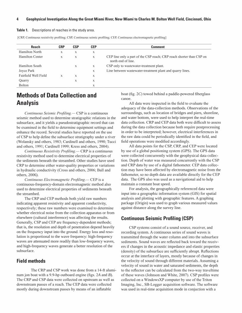
Table 1. Descriptions of reaches in the study area.

[CRP, Continuous resistivity profiling; CSP, Continuous seimic profiling; CEP, Continuous electromagnetic profiling]

Reach CRP CSP CEP CommentHamilton North x x xHamilton Center x x x CEP line only a part of the CSP reach; CRP reach shorter than CSP on

north end of line.Hamilton South x x CSP only to wastewater-treatment plant.Joyce Park x Line between wastewater-treatment plant and quarry lines.Fairfield Well Field x x xQuarry x xBolton x

Methods of Data Collection and Analysis 5

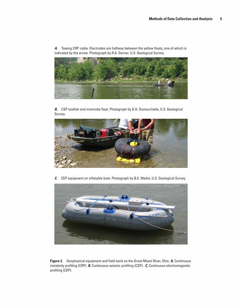
Figure 2. Geophysical equipment and field work on the Great Miami River, Ohio. A, Continuous resistivity profiling (CRP). B, Continuous seismic profiling (CSP). C, Continuous electromagnetic profiling (CEP).

A. Towing CRP cable. Electrodes are halfway between the yellow floats, one of which is indicated by the arrow. Photograph by R.A. Darner, U.S. Geological Survey.

B. CSP towfish and innertube float. Photograph by D.H. Dumouchelle, U.S. Geological Survey.

C. CEP equipment on inflatable boat. Photograph by B.E. Mailot, U.S. Geological Survey.


control unit and a towfish (model SB-2165), containing the seismic source and two receivers, manufactured by EdgeTech. This CSP system is a swept-frequency (chirp) system that sweeps through a series of frequencies between 2 and 16 kHz. The signal is transmitted to the control unit, displayed on a monitor, and stored digitally.

The CSP towfish is designed to be submerged below the water surface and towed behind the boat to minimize interfer-ence and ringing between the boat and water bottom. Because of the shallow depth of the Great Miami River, the towfish was secured to and floated by a tractor-tire innertube and towed at the surface beside the boat (fig. 2B). The towfish, seismic control unit, and laptop computer were powered by a portable generator. The start and end times of each survey line, the boat speed, the water depth, and the shooting parameters were recorded on field sheets. The locations of potential side reflectors such as bridge piers or debris also were recorded. The towfish produced a “noisy” bow wave when being towed upstream, particularly in strong currents. Efforts such as minimizing the boat speed, altering the angle of the boat to the current, and adjusting the innertube-to-towfish tielines were used to reduce the bow wave. Transmission was typically 2 or 4 times per second and recording length from 40 to 100 milliseconds, which is approximately equivalent to a depth of 30 to 75 m of water and sediment.

The reflection data were presented as a series of traces showing the varying amplitudes as a function of traveltime. The consecutive traces are plotted next to one another, and as a group form a pseudo cross section of the subsurface. Indi-vidual reflectors can be traced along this seismic cross section and correlated to boreholes and geologic cross sections. The air-water and the water-sediment interfaces have very high differences in acoustic impedance (high contrast); therefore, reflections from these interfaces are typically very strong. Point reflectors (diffractors) and linear reflectors are typically identified on the trace records and interpreted. The character of reflection patterns also can be used to infer the composition of the bottom and subsurface; for example, a chaotic, discontinu-ous, diffracted pattern for the water-sediment reflector may indicate a coarse gravel or boulder bottom (Haeni, 1988; Pow-ers and others, 1999).

Postprocessing to display and interpret the CSP data was done with DelphMap (Triton Imaging, Inc.) and associated software packages. Filters and gains were applied to enhance the images and were selected by trial and error. A high-pass fil-ter was set at 1,250 Hz and low-pass filter at 6,250 Hz to help reduce unwanted high and low frequencies that obscured sub-surface reflectors. In addition, automatic gain control was used to enhance later time signals. Stacking was used to enhance coherent reflectors. Various color schemes and scales were used by trial and error to enhance subtle features to facilitate interpretation of geologic information.

Continuous Resistivity Profiling (CRP)

CRP is based on the same principles as land-based elec-trical resistivity profiling. Resistivity is an intrinsic property of a microscopic volume of the sediment. CRP measures the apparent resistivity, which is a volume-averaged resistivity. An electrical current is injected into the earth/water body through two current electrodes, and the voltage differences are mea-sured across various pairs of potential electrodes. The apparent resistivity of the water and subsurface is directly proportional to the geometry of the electrode array and the voltage differ-ence and is inversely proportional to the applied current. The apparent resistivity for each potential electrode pair is plot-ted at the midpoint distance between the electrodes, and the pseudo depth is plotted as a function of the distance between the electrodes in a pseudo cross section of the profile. For CRP, current is applied and voltage is measured continuously along the electrode array as the array (streamer) is advanced through the water with a boat.

An eight-channel Advanced Geosciences, Inc., Super Sting was used to collect the CRP data. For this investigation, 11 electrodes spaced 5 m apart were towed behind the boat; the yellow floats in figure 2A were midway between the elec-trodes. The cable available for this study had electrodes spaced 10 m apart; but because the longer the electrode spacing would have had a greater depth penetration, a shorter, 5-m spacing was preferred for this study. The cable was coiled and taped to itself between the electrodes to obtain the 5-m spacing. The two electrodes closest to the boat injected current, and eight potential measurements were made with the nine remaining electrodes, approximately every 2–3 seconds. A dipole-dipole electrode array was used for the profiles described herein (Johnson and White, 2007, fig. 4). No stacking or reciprocal measurements were done, owing to movement of the boat.

The start and end times of each survey line and boat speed were recorded on field sheets. The specific conductance of the water, in microsiemens per centimeter at 25 degrees Celsius (µS/cm at 25°C), was recorded at least once on each reach. The locations of potential sources of interference, such as powerlines and bridges, were recorded as well.

The GPS navigational data were synchronized with the CRP data within the software Marine Log Manager (Advanced Geosciences, Inc). The combined GPS and CRP data were saved in sections for further processing. Postprocessing of the CRP section data was done with the RES2DINV software package (Loke, 2007). The data were plotted in apparent resistivity pseudo sections and examined for excessive noise. Data points deemed to be above background were deleted manually. In general, less than 3 to 5 percent of the data were removed for being outside a reasonable range. Each data section was inverted from apparent resistivity to resistivity in order to determine a subsurface model response of water and sedimentary material that best matched the measured apparent-resistivity data, within certain constraints. After each iteration of the model, the inverse model section (computed data) is compared numerically with the apparent-resistivity

Results of Continuous Profiling of Subsurface Characteristics 7

section (measured data); when the differences between the two sections are within user-specified criteria, iterations stop. Both unconstrained and constrained inversions were done on each section. Unconstrained inversions, where the resistivity and thickness of the water column were unconstrained in the model, were examined to ensure that resistivity of the water column was similar across sections and that the depth of water did not change abruptly. If abnormalities existed in the uncon-strained inversion, problems with the constrained inversion would result; fortunately, no abnormalities were found in any of the unconstrained inverstions. For the constrained inver-sions, the water layer in the model was set to 12.12 ohm-m. The specific conductance of the water was approximately 825 mS/cm (see conversion factor on page iv). The inversions are based on the assumption that the resistivity of the river water was constant through the water column.

Continuous Electromagnetic Profiling (CEP)

Continuous electromagnetic profiling was used to mea-sure changes in apparent electrical conductivity with position and depth along the river. In this environment, changes in apparent electrical conductivity could relate to characteristics of rock type (sand, gravel, clay), water quality or, to a lesser extent, temperature. Because the water quality of the water column is well mixed, and the assumption can be made that the water quality in the shallow subsurface under the river is similar in terms of electrical properties, the method was used to examine changes in rock type along the reaches surveyed. It should be noted, however, that the above assumption may not be uniformly appropriate.

Measurements were made with a the Geophex, Incor-porated, GEM-2, a hand-held, digital, multifrequency elec-tromagnetic-induction instrument (Won and others, 1996; Huang and Won, 2000). The GEM-2, which was operated in a frequency range of 330 Hz to 24 kHz, contains three coils: transmitter (Tx), bucking, and receiver (Rx). The Tx and Rx coils have a fixed separation distance of about 1.7 m and are molded into a single boom that allows an individual to carry the instrument easily. The GEM-2 generates a multiple-fre-quency waveform that takes advantage of the electromagnetic skin-depth. Because skin-depth is inversely proportional to frequency, a low frequency can sample deeper than a high frequency can (Won and others, 1996; White and others, 2005). The depth of exploration or penetration is related to the electromagnetic skin-depth.

For this study, three frequencies (750; 3,510; and 15,030 Hz) were collected on the data logger at approximately equal intervals of 0.1 second (10 Hz). The antenna and data logger (ski) was placed in a rubber raft, which was towed about 10 ft behind a fiberglass canoe (fig. 2C). Batteries and electronics were placed in the canoe to minimize interference. The data logger generally was kept parallel to the path of travel and, for the most part, the raft towed straight behind the canoe. However, in some river bends, the current would pull the raft

out of line from the canoe for a short distance. For the Ham-ilton, Fairfield, and Quarry reaches, the CEP data-collection lines were similar to the lines of the CRP and CSP data; but for the Joyce Park and Bolton reaches, data were collected generally from the center of the river as the current allowed. Operational procedures recommended in the GEM-2 manual (Geophex, 2004), such as warming up receiver before data collection, were followed. The GEM-2 and GPS data were downloaded to a laptop in the field by use of the program WinGEMv3 (Geophex, 2003), which generates a binary-for-mat file containing data collected by the GEM-2. The apparent conductivity for each frequency was calculated from these data and the GPS position of the data points. All data were exported to ASCII files for further processing.

Because of the large number of data points collected in the field, the apparent-conductivity data for each frequency and each separate section of data were filtered with a running-average filter of 1 second (approximately 4 ft) and compiled into a single spreadsheet. The spreadsheet facilitated data input into a GIS and graphing packages.

Results of Continuous Profiling of Subsurface Characteristics

The following sections summarize the results of data analysis for the CSP, CRP, and CEP data. Detailed datasets, including geographic information for each data point, are available upon request.

CSP

Water depth and difficulty with mobilizing the heavy transducer limited the CSP survey lines to areas where the transducer could float safely (fig. 3). The raw and processed CSP data are available on request.

Generally, the CSP lines were of poor quality, primarily because of the current, wave action, and the bow wave from the boat used to tow the transducer. These factors created vertical “ringing” in the record. The processing of the records seemed to eliminate this high-frequency ringing, but it also may have eliminated high-frequency reflections in the subsur-face. Strong multiple reflections (“multiples”) from the stream bottom were evident in nearly every profile, which obscured most of the shallow (<5 m) subsurface reflections. Water-bot-tom multiples occur as the signal is reflected off an acousti-cally reflective surface, such as rock, compacted sediments, or entrapped gas. Little can be done to remove the effects of multiples on single-channel data. Some deeper (>5 m) reflec-tions were seen in a few of the profiles.

Several of the records give indications of the type of bot-tom material of the river bottom, indicating some horizontal layering in the shallow (<10 cm) subsurface of the river.


Figure 3. Location of continuous seismic profiles.


Figure 4. Location of continuous resistivity profiles.


Very few, if any, coherent reflections were seen below a few centimeters of the river bottom in either the raw or processed CSP records. This absence of reflections could be due to lack of penetration of the seismic signal, to attenuation, to exces-sive interference, or to a combination of these factors.

CRP

CRP survey lines were run along the Hamilton-North, the Hamilton-Center, and the Fairfield Well Field reaches of the study area (figs. 1 and 4). All lines were inverted to less than 5 percent agreement between the apparent resistivity observa-tions and the inverted resistivity. The modeled cross sections showing the results of the inversions are available on request.

Because a 5-m electrode spacing was used during data collection, no inversion results are available between 0 and about 1 m below the stream bottom for each model section. Various levels of interference show in each modeled section due to overhead powerlines, bridges, or roads. Sources of cultural interference were noted in the field, so they were rela-tively easy to identify in the model cross sections. Repeatabil-ity of the data collection and the model results was seen when comparing data from line FWF1 and the first 200 m of FWF2; the two lines were collected on nearly identical profiles.

Every model section shows a distinct change between shallow (less than about 5 m) and deep (greater than about 5 m) modeled resistivity. Previous studies in the Hamilton area (Sheets and Bossenbroek, 2005) indicate a discontinu-ous till between 6 and 8 m depth at the Hamilton North Well Field, but till is likely shallower near the river (Sheets and Bossenbroek, 2005, fig. 3). The modeled resistivities were grouped in various depth categories, and the largest difference was found between those modeled resistivities less than 3.3 m and greater than 3.3 m below the stream bottom (fig. 5). The average resistivity at depths less than 3.3 m below the stream bottom was 310 ohm-m; average resistivity at depths greater than 3.3 m below the stream bottom was 66 ohm-m. Figure 6 shows the modeled (log) resistivities less than 3.3 m below the stream bottom along the Great Miami River and indicates a rather large variation of shallow apparent electrical resistivi-ties, even from one side of the river to another. The north and west areas of the Hamilton-North reach seem to have lower resistivities than the south and east areas. The northern area of the Hamilton-Center reach has much lower resistivities overall than the southern part of the reach, indicating a finer grained material at shallow depths.

Higher electrical resistivity (250 ohm-m) generally indicates a predominance of sand/gravel, and lower electrical resistivity (less than 100 ohm-m) generally indicates a finer grained material (clay). Generally, shallow electrical resistiv-ity (at depths less than about 3.5 m below the stream bottom) ranged from about 300 to 1,500 ohm-m, indicating geologic materials from clay to sand and gravel. Variations in resistiv-ity can be seen in shallow sections of every modeled profile, but the resolution is relatively coarse because of the electrode spacing and resulting spatial coverage of shallow material.

CEP

The entire reach of the Great Miami River between New Miami and Bolton Well Field was surveyed with CEP. Figure 7 shows the 750-Hz filtered data. The filtered data for 750, 3,510, and 15,030 Hz along the entire reach are shown in graphical form in figures 8, 9, and 10, respectively. The 750-Hz data show clearly the effects of cultural interference (overhead railways, roads, powerlines), as evidenced by much higher electrical conductivities than the “base” values of less than 10 mS/m. These interferences can be seen in figure 8, between kilometer 2.6 and 4.8 and sporadically thereafter. The 3,510 and 15,010 Hz data are very similar to each other and have a much higher base value (between 20 and 90 mS/m) than the 750-Hz data (figs. 9 and 10). The high-frequency data (3,510 and 15,030 Hz) also show some effects of cultural interference.

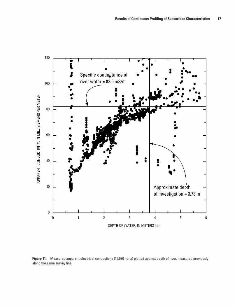
Because of the water depth and specific conductance (about 825 mS/cm or 82.5 mS/m) of the Great Miami River, the apparent-conductivity data were analyzed to determine whether the combination of water depth and specific con-ductance affected the depth of penetration through the water column. By means of GIS, the location of the CEP line was intersected with the water-depth information obtained from the CRP lines (within 6 m of the line), because water-depth information was not collected during the CEP data collec-tion. Figure 11, which shows the measured apparent electrical conductivity (15,030 Hz) plotted against the depth of water, indicates that at water depths greater than about 3.8 m, the measured apparent conductivity is approximately 82.5 mS/m. The mean of measured apparent conductivity below 3.8 m is 82.5 mS/m, which corresponds to the equivalent units of specific conductance of the river. Plots of the 3,510-Hz data looked very similar to plots of the 15,030-Hz data, but no correlation was observed between water depth and apparent electrical conductivity for the 750-Hz data.

Using equation 5, from Huang (2005) a depth of investi-gation1 was calculated through water at specific conductance of 82.5 mS/m. To calculate the depth of investigation, a detec-tion threshold (T) was calculated to be 2.5 times the standard deviation of the data from deeper than 3.8 m (T equals 31 percent). The calculated depth of investigation was 3.8 m. At depths of investigation shallower than about 3.8 m, the appar-ent-conductivity response for this frequency is from the water column and the bottom/subsurface material. At depths greater than 3.8 m, the apparent-conductivity response is strictly from the water column. Therefore, the apparent-conductivity data for frequencies 3,510 and 15,030 Hz (figs. 9 and 10) consist of responses from varying amounts of water and sediment, and the response depends on depth of water.

1 The depth of investigation in electromagnetic soundings is a maximum depth at which a given target in a given host can be detected by a given sensor.


Figure 5. Frequency plot of modeled resistivity along the Great Miami River, from Hamilton to Bolton Well Field. The average (log) resistivity at modeled depths greater than 3.3 meters is markedly lower than the (log) resistiviy less than 3.3 meters. Resistivities greater than 3,000 ohm-meters were removed and are likely due to interference, contact resistance, or measurement error.


Figure 6. Model-derived apparent (log) resistivity for depths between 0 and 3.3 meters beneath stream bottom.


Figure 7. Continuous electromagnetic profile locations and apparent conductivity along the Great Miami River.


Figure 8. Electrical conductivity measured with the GEM-2 at 750 hertz, along the Great Miami River from Hamilton North Well Field to Bolton Well Field.


Figure 9. Electrical conductivity measured with the GEM-2 at 3,510 hertz, along the Great Miami River from Hamilton North Well Field to Bolton Well Field.


Figure 10. Electrical conductivity measured with the GEM-2 at 15,030 hertz, along the Great Miami River from Hamilton North Well Field to Bolton Well Field.


Figure 11. Measured apparent electrical conductivity (15,030 hertz) plotted against depth of river, measured previously along the same survey line.


In general, the apparent electrical conductivity at 750 Hz is somewhat higher north of mile 4 (Hamilton-North and Hamilton-Center reaches) than in the south (Hamilton-South, Fairfield Well Field, and Bolton reaches), indicating that the sediments upstream from the low-head dam are probably more fine grained than downstream from the low-head dam. A slight increase in the electrical conductivity (750 Hz) near the Bolton reach indicates a possible decrease in grain size. Because the CRP and CEP are measuring electri-cal properties of the subsurface, a cursory examination of the

relations between the results is in order. Figure 12, a plot of apparent conductivity of the CRP model results (inverse of resistivity) for increasing electrode-spacing (dipole-dipole spacing) against the total electromagnetic conductivity from the CEP, it shows that the total CEP response is best cor-related with the small electrode spacings (less than 10 m) or the shallowest CRP response. The CRP data were biased to deeper sediments when compared with the CEP data; thus, an electrode spacing of less than 5 m would be needed to get a stronger correlation with the CEP data.

Figure 12. Apparent conductivity from resistivity survey plotted against total electromagnetic conductivity field data.

Summary and Conclusions 19

Suggested Method Modifications for Future Work of This Type

Because of the draft and bulkiness of the boat that has to be used on this waterway and the somewhat fragile nature of the CSP transducer used in the study, the areas available for surveying on this river were limited. The logistics of float-ing the transducer at the water surface also degraded the data quality. If a smaller, more portable and rugged transducer were available that could be towed behind the boat, perhaps the acoustical “ringing” could be eliminated and better data could be collected.

In this study, a 5-m electrode spacing was used for the CRP surveys, which resulted in an approximately 60-m strand of cables floating behind the boat. The cable used had 10-m electrode spacing but was modified in the field to accommo-date 5-m spacing, resulting in extra cable lengths between the electrodes. The sinuosity of the river, boat access, and cable issues limited the areas where surveys could be done. A shorter (less than 5-m) CRP electrode spacing would enhance shallow measurements and analysis. We suggest that cable with 3-m electrode spacing (possibly even shortened to 1 m) be used in similar environments to determine shallow (less than 3-m) electrical properties of the stream-bottom materials.

Additional CEP work could be done at sites similar to the study area, but we suggest that more frequencies be collected at a slower rate (approx. 1 second). Because of the depth of pen-etration through the relatively high-specific-conductance (low-resistivity) water, frequencies at low end of the CEP frequency spectrum (approximately 330 Hz to 1.5 kHz) should be used to maximize depth of penetration through the water column and subsurface materials.

The water depth in CEP study reaches should be mea-sured concurrently with a fathometer. Testing should be done to minimize interference from the fathometer; if possible, the fathometer should be placed on the guide boat instead of the boat for the equipment and translated on processing to the locations of CEP measurements. Additionally, a continuous record of specific conductance and temperature could also be obtained during CEP passes. If such data were collected, depth and resistivity of water along the profile lines would be known, and a relatively straightforward inversion of the data could be applied to determine electrical resistivity of the subsurface materials.

Some of the data collected during this investigation may be useful in conjunction with concurrent work by the Miami University. The Miami University data, derived from seepage-meter measurements and temperature monitoring, could provide small-scale (local) estimates of riverbed hydraulic characteristics. The geophysical data from this study, while covering a much larger area of the riverbed, is less specific about hydraulic characteristics. Comparing and contrast-ing the two datasets may provide additional insights into the characteristics of the Great Miami River, as well as possibly

extrapolating information to areas where seepage-meter and temperature measurements could not physically be obtained. Additional streamflow, sediment, and riverbed-characteristic studies could be useful in comparing data from this study and the Miami Univeristy work.

Summary and ConclusionsThe siting of several well fields along the Great Miami

River in southwest Ohio has led to several previous and ongo-ing studies of surface-water/ground-water interactions. In the study described in this report, three waterborne geophysical profiling methods were tested to evaluate their effectiveness and to help characterize subsurface materials at selected tran-sects along the Great Miami River. The profiling methods used were continuous seismic profiling (CSP), continuous resistiv-ity profiling (CRP), and continuous electromagnetic profiling (CEP). Data collection involved the use of global positioning systems to spatially locate the data along the river.

The depth and flow conditions of the Great Miami River limited the boat access, flotation of the CSP transducer, and the amount and quality of data that could be collected with the CSP method. In addition, the shallow river depth neces-sitated towing the CSP equipment in a manner that may have contributed to excessive interference. Shallow reflections (less than 5 m) were mostly obscured by strong multiple reflections indicative of an acoustically hard water bottom. Deep reflec-tions (greater than 5 m) were sparse and discontinous.

CRP data collection also was limited by water depth, flow conditions, and boat access. However, inverse modeling of CRP data indicated broad changes in subsurface geology, primarily below about 3 to 5 m. Where CRP data were col-lected, interpretations were consistent with previous studies along the Great Miami River and showed a discontinuous till along with lower and upper aquifers. Detailed shallow (less than 3-m) electrical conductivity (resistivity) data were limited because of the 5-m electrode spacing used for the surveys. For future studies of this type, a cable with 3-m electrode spacing (or perhaps even 1-m spacing) might best be used in similar environments to determine shallow (less than 3-m) electrical properties of the stream-bottom materials.

CEP data were collected along the entire reach of the Great Miami River. The CRP and CEP data did not correlate well, but the CRP electrode spacing probably limited the cor-relation. Middle-frequency (3,510 Hz) and high-frequency (15,030 Hz) CEP data were correlated to water depth. Low-frequency (750 Hz) CEP data sampled deeper than the water column and were consistent with shallow (less than 5-m) changes in electrical conductivity along this reach of the Great Miami River. Because of the impact of the water column on the CEP results, numerical modeling of the CEP data would be necessary to determine true electrical conductivity of the streambed and underlying geologic materials. However, the CEP profiles can be used to infer hydraulic properties along


the stream bottom, based on inferences of electrical response of geologic materials. Given the variability in depth and flow conditions on a river such as the Great Miami, the CEP method worked better than either the CSP or CRP methods.

The character of the CRP sections and the CEP data between the upstream section (Hamilton North well field) and downstream section (Bolton Well Field) seems to indicate some general changes in geologic character of the stream bot-tom and/or subbottom. The upstream CRP sections indicate a discontinuous, electromagnetically conductive layer a few meters below the stream bottom; the 750 Hz CEP data indicate a higher overall electromagnetic signal than do the middle or downstream datasets. A discontinuous till layer that would be consistent with these results was identified underlying the Hamilton North well field in a previous study (Sheets and Bossenbroek, 2005). Because of the absence of these high-conductivity (low-resistivity) signals in the middle part of the section (Hamilton to Fairfield Well Field), this till layer may be either missing, more discontinuous, or below the detection of the instruments. The downstream electromagnetic profile (Hamilton South Well Field to Bolton Well Field) seemed to indicate a general increase in the electromagnetic signal and a slightly different character than the modeled resistivity pro-files, indicating an increase in clay (more conductive) content. There was no indication that a coherent clay (till) layer was present to cause this result. It would be interesting to relate these results to depositional models of the valley fill material and to streambed-sediment deposition (velocity profiles of the Great Miami River).

AcknowledgmentsThe authors thank Bruce Whitteberry (City of Cincin-

nati), Tim McLelland (Hamilton to New Baltimore Ground Water Consortium), and William Gollnitz (previously of the City of Cincinnati) for valuable assistance in getting this project started. In addition, Tim McLelland was of valuable assistance in finding locations to deploy the boat. The authors also thank the Miami Conservancy District (MCD) and James Sharn at Martin Marietta for providing river access.

References Cited

Ball, L.B., Kress, W.H., Steele, G.V., Cannia, J.C., and Ander-sen, M.J., 2006, Determination of canal leakage potential using continuous resistivity profiling techniques, Interstate and Tri-State Canals, western Nebraska and eastern Wyo-ming, 2004: U.S. Geological Survey Scientific Investiga-tions Report 2006–5032, 53 p.

Cardinell, A.P., 1999, Application of continuous seismic-reflection techniques to delineate paleochannels beneath the Neuse River at U.S. Marine Corps Air Station Cherry Point, North Carolina: U.S. Geological Survey Water-Resources Investigations Report 99–4099, 29 p.

Cardinell, A.P., Harned, D.A., and Berg, S.A., 1990, Continu-ous seismic reflection profiling of hydrogeologic features beneath New River, Camp Lejeune, North Carolina: U.S. Geological Survey Water-Resources Investigations Report 89–4195, 33 p.

Cross, V.A.; Bratton, J.F.; Bergeron, Emile; Meunier, J.K.; Crusius, John; and Koopmans, Dirk, 2006, Continuous resistivity profiling data from the Upper Neuse River Estu-ary, North Carolina, 2004–2005: U.S. Geological Survey Open-File Report 2005–1306, 1 CD-ROM.

Dumouchelle, D.H., 1998a, Ground-water levels and flow directions in the buried valley aquifer around Dayton, Ohio, September 1993: U.S. Geological Survey Water-Resources Investigations Report 97–4255, 1 sheet, scale 1:100,000.

Dumouchelle, D.H., 1998b, Simulation of ground-water flow, Dayton area, southwestern Ohio: U.S. Geological Survey Water-Resources Investigations Report 98–4048, 57 p.

Geophex, Ltd., 2003, WinGEMv3 (computer program): Raleigh, N.C., available online at www.geophex.com (accessed December 2007).

Geophex, Ltd., 2004, GEM-2 manual, version 3.8: Raleigh, N.C., 22 p., available online at www.geophex.com (accessed December 2007).

Haeni, F.P., 1988, Evaluation of the continuous seismic-reflec-tion method for determining the thickness and lithology of stratified drift in the glaciated Northeast, in Randall, A.D., and Johnson, A.I., eds., Regional aquifer systems of the United States—The northeast glacial aquifers: Bethesda, Md., American Water Resources Association Monograph Series 11, p. 63–82.

Huang, Haoping, 2005, Depth of investigation for small broadband electromagnetic sensors: Geophysics, v. 70, no. 6, p. G135–G142.

Huang, Haoping, and Won, I.J., 2000, Conductivity and susceptibility mapping using broadband electromagnetic sensors: Journal of Environmental and Engineering Geophysics, v. 5, no. 4, p. 31–41.

Johnson, C.D., and White, E.A., 2007, Marine geophysical investigation of selected sites in Bridgeport Harbor, Con-necticut, 2006: U.S. Geological Survey Scientific Investi-gations Report 2007–5119, 32 p.

References Cited 21

Klaer, F.H., Jr., and Thompson, D.G.,1948, Ground-water resources of the Cincinnati area, Butler and Hamilton Coun-ties, Ohio: U.S. Geological Survey Water-Supply Paper 999, 168 p.

Kress, W.H., Dietsch, B.J., Steele, G.V., White, E.A., and Cannia, J.C., 2004, Use of continuous seismic profiling to differentiate geologic deposits underlying selected canals in central and western Nebraska: U.S Geological Survey Fact Sheet 03–115, 6 p.

Loke, M.H., 2007, RES2DINV ver. 3.56 for Windows 98/Me/2000/NT/XP—Rapid 2-D resistivity and IP inver-sion using the least-squares method: Penang, Malaysia, Geotomo Software, 138 p., available online at http://www.geoelectrical.com (accessed December 1, 2007).

Powers, C.J., Haeni, F.P., and Smith, Spence, 1999, Inte-grated use of continuous seismic-reflection profiling and ground-penetrating radar methods at John’s Pond, Cape Cod, Massachusetts: Tulsa, Okla., Society of Exploration Geophysicists, Symposium on the Application of Geophys-ics to Engineering and Environmental Problems (SAGEEP), v. 12, no. 1, p. 359–369.

Rowe, G.L, Jr., Reutter, D.C., Runkle, D.L., Hambrook, J.A., Janosy, S.D., and Hwang, L.H., 2004, Water quality in the Great and Little Miami River Basins, Ohio and Indiana, 1999–2001: U.S. Geological Survey Circular 1229, 40 p.

Sheets, R.A., 2007, Hydrogeologic setting and ground-water flow simulations of the Great Miami River Basin regional study area, Ohio, in Paschke, S.S., ed., Hydrogeologic set-tings and ground-water flow simulations for regional studies of the Transport of Anthropogenic and Natural Contami-nants to public-supply wells—Studies begun in 2001: U.S. Geological Survey Professional Paper 1737–A, p. 7–1 to 7–23.

Sheets, R.A., and Bossenbroek, K.E., 2005, Ground-water flow directions and estimation of aquifer hydraulic proper-ties in the lower Great Miami River buried valley aquifer system, Hamilton, Ohio: U.S. Geological Survey Scientific Investigations Report 2005–5013, 31 p.

Sheets, R.A., Darner, R.A., and Whitteberry, B.L., 2002, Lag times of bank filtration at a well field, Cincinnati, Ohio, USA: Journal of Hydrology, v. 266, nos. 3–4, p. 162–174.

Spieker, A.M., 1968, Ground-water hydrology and geology of the lower Great Miami River Valley, Ohio: U.S. Geological Survey Professional Paper 605–A, 37 p.

Tucci, Patrick, Haeni, F.P., and Bailey, Z.C., 1991, Delineation of subsurface stratigraphy and structures by a single channel continuous seismic-reflection survey along the Clinch River, near Oak Ridge, Tennessee: U.S. Geological Survey Water-Resources Investigations Report 91–4023, 27 p.

White, E.A., Thompson, M.D., Johnson, C.D., Abraham, J.D., Miller, S.F., and Lane, J.W., Jr., 2005, Surface-geophysical investigation of a formerly used defense site, Machiasport, Maine, February 2003: U.S. Geological Survey Scientific Investigations Report 2004–5099, 48 p.

Wolanksy, R.M., Haeni, F.P., and Sylvester, R.E., 1983, Con-tinuous seismic-reflection survey defining shallow sedi-mentary layers in the Charlotte Harbor and Venice areas, southwest Florida: U.S. Geological Survey Water-Resources Investigations Report 82–57, 77 p.

Won, I.J., Keiswetter, D.A., Fields, G.R.A., and Sutton, L.C., 1996, GEM-2—A new multifrequency electromagnetic sen-sor: Journal of Environmental and Engineering Geophysics, v. 1, no. 2, p. 129–138.

Sheets and Dumouchelle—

Geophysical Investigation A

long the Great M

iami River, N

ew M

iami to Cincinnati, O

hio—Open-File Report 2009–1025

geophysical investigation along the great miami river · pdf filegeophysical investigation...

Documents