geophysical journal international - uwyo.edulwang7/papers/jgeophysical2011.pdf · 1department of...

Geophys. J. Int. (2011) 186, 311–330 doi: 10.1111/j.1365-246X.2011.05031.x

GJI

Sei

smol

ogy

Rapid full-wave centroid moment tensor (CMT) inversion ina three-dimensional earth structure model for earthquakesin Southern California

En-Jui Lee,1 Po Chen,1 Thomas H. Jordan2 and Liqiang Wang3

1Department of Geology and Geophysics, University of Wyoming, WY 82071, USA. E-mail: [email protected] of Earth Sciences, University of Southern California, CA, USA3Department of Computer Science, University of Wyoming, WY 82071, USA

Accepted 2011 March 31. Received 2011 March 31; in original form 2010 October 2

S U M M A R YA central problem of seismology is the inversion of regional waveform data for models ofearthquake sources. In regions such as Southern California, preliminary 3-D earth structuremodels are already available, and efficient numerical methods have been developed for 3-Danelastic wave-propagation simulations. We describe an automated procedure that utilizesthese capabilities to derive centroid moment tensors (CMTs). The procedure relies on theuse of receiver-side Green’s tensors (RGTs), which comprise the spatial-temporal displace-ments produced by the three orthogonal unit impulsive point forces acting at the receivers. Wehave constructed a RGT database for 219 broad-band stations in Southern California usinga tomographically improved version of the 3-D SCEC Community Velocity Model Version4.0 (CVM4) and a staggered-grid finite-difference code. Finite-difference synthetic seismo-grams for any earthquake in our modelling volume can be simply calculated by extracting asmall, source-centred volume from the RGT database and applying the reciprocity principle.The partial derivatives needed for the CMT inversion can be generated in the same way. Wehave developed an automated algorithm that combines a grid-search for suitable focal mech-anisms and hypocentre locations with a Gauss–Newton optimization that further refines thegrid-search results. Using this algorithm, we have determined CMT solutions for 165 smallto medium-sized earthquakes in Southern California. Preliminary comparison with the CMTsolutions provided by the Southern California Seismic Network (SCSN) shows that our solu-tions generally provide better fit to the observed waveforms. When applied to a large numberof earthquakes, our algorithm may provide a more robust CMT catalogue for earthquakes inSouthern California.

Key words: Probability distributions; Earthquake ground motions; Earthquake source ob-servations; Computational seismology; Wave propagation; Early warning.

1 I N T RO D U C T I O N

Accurate and rapid seismic source parameter inversions are important for seismic hazard analysis in earthquake-prone areas such as SouthernCalifornia. The Southern California Seismic Network (SCSN) routinely determines the focal mechanisms from first-motion polarities forearthquakes with local magnitude as low as 2.0–2.5 (Hauksson 2000). With the advancement of digital broad-band instrumentation, completeCentroid Moment Tensor (CMT; Dziewonski et al. 1981) solutions can be automatically recovered from regional broad-band waveformdata for earthquakes with local magnitude larger than 3.0 (Dreger & Helmberger 1991; Zhao & Helmberger 1994; Thio & Kanamori 1995;Pasyanos et al. 1996; Zhu & Helmberger 1996; Liu et al. 2004; Clinton et al. 2006).

In the waveform inversion approach, an optimal CMT solution is found by minimizing a certain measure of the waveform misfit betweenobserved and model-predicted (synthetic) seismograms either in time domain (e.g. Zhao & Helmberger 1994; Zhu & Helmberger 1996) or infrequency domain (e.g. Romanowicz et al. 1993; Thio & Kanamori 1995). To reduce computational cost, synthetic seismograms as well astheir partial derivatives with respect to CMT parameters are often computed in simple 1-D earth structure models using semi-analytic methods(e.g. Zhao & Helmberger 1994; Dreger 2003). Multiple 1-D structure models can be adopted to account for gross lateral variations in crustalstructure. And phases that are relatively insensitive to crustal heterogeneities, such as long-period surface waves and Pnl, the combinationof Pn and PL (Helmberger & Engen 1980), can be used in the inversion to alleviate the dependence on structure models. Difficulties may

C© 2011 The Authors 311Geophysical Journal International C© 2011 RAS

Geophysical Journal International

312 E.-J. Lee et al.

arise when attempting inversions for smaller earthquakes, as the signal-to-noise ratio (SNR) at long periods may become too low for smallerearthquakes (Mw ≤ 3.7). For inversions at shorter periods, small-scale lateral variations in crustal structure can become important and tofurther accommodate those small-scale structural variations, simple time shifts between portions of observed and synthetic seismograms areallowed while minimizing the waveform misfit (e.g. Zhao & Helmberger 1994; Zhu & Helmberger 1996).

Recent advances in parallel computing technology and numerical methods (Olsen 1994; Graves 1996; Akcelik et al. 2003; Olsen et al.2003; Komatitsch et al. 2004) have made large-scale 3-D numerical simulations of seismic wavefields much more affordable, and theyopen up the possibility of using highly accurate synthetic Green’s functions computed in 3-D earth structure models in source parameterinversions. Synthetic Green’s functions computed from a good 3-D earth structure model can account for complex wave phenomena andreduce phase differences with observed waveforms. Ramos-Martınez & McMechan (2001) developed a full-waveform focal mechanisminversion algorithm that uses synthetic Green’s functions computed for a 3-D heterogeneous viscoelastic anisotropic structure model usinga staggered-grid finite-difference method and applied it to two aftershocks of the 1994 Mw 6.7 Northridge earthquake. They found thatincorporation of realistic 3-D structure reduced the residual errors of the waveform fitting by more than 50 per cent compared to those for a1-D layered model. In their algorithm, source locations are not inverted. Liu et al. (2004) developed a full-waveform CMT inversion techniqueusing synthetic Green’s functions computed in the 3-D Harvard crustal structure model for Southern California (Suss & Shaw 2003) basedon the spectral-element method (Komatitsch et al. 2004). The partial derivatives of the synthetic waveforms with respect to the six momenttensor components and the source location were evaluated numerically through differencing. Up to 10 wave-propagation simulations wereneeded to calculate all partial derivatives. When the initial location is far from the true location, non-linear, iterative optimization algorithmscan be adopted but the computational cost can become quite high for obtaining a robust solution in a short period of time after the earthquake.A similar approach has been recently adapted to continental scale in Hingee et al. (2010) using a 3-D structure model for the Australasianregion obtained through full-wave adjoint tomography (Fichtner et al. 2009; Fichtner et al. 2010). A number of sensitivity tests show that the3-D model is superior to a well-calibrated 1-D model in obtaining accurate CMT solutions.

As numerical simulations of seismic wavefields in 3-D structure models are still computationally intensive, if we perform forwardsimulations for every potential source model, it is very impractical for rapid or (near) real-time applications. A more practical approach forrapid CMT inversions in a 3-D earth structure model is to use the reciprocity principle (Aki & Richards 2002; Okamoto 1994a,b; Okamoto2002). Zhao et al. (2006) introduced the use of receiver Green’s tensors (RGTs) for source parameter inversions in 3-D earth structure modelsby taking advantage of the reciprocity principle. The RGTs are the strain fields, as functions of both space and time, generated by threeorthogonal unit impulsive point forces acting at the receiver locations. By applying the reciprocity principle, it can be shown that the RGTsprovide exact partial derivatives of the waveforms at the receiver locations with respect to the moment tensor at any point in the modellingvolume. The RGTs can be calculated with high accuracy in a 3-D earth structure model using numerical methods, such as finite-difference,finite-element and spectral-element methods, and stored in a database. Since the synthetic seismograms and their partial derivatives canbe retrieved from the database very rapidly, the RGT-based approach is better suited for (near) real-time source parameter inversions. Thedisadvantage of this approach is that since the RGT database has to be constantly on-line for rapid access, the disk storage cost could be quitehigh. The computational and storage costs for CMT inversions using RGTs calculated in a 3-D structure model for the Los Angeles basinregion based on the finite-difference method were summarized in Chen et al. (2007). Traditional high-performance computing platformssuch as distributed-memory computer clusters are usually shared by multiple users and suffer from long delays in acquiring computationalresources. The emerging cloud computing platform allows users to acquire and release resources on-demand with very low schedulingoverheads and may provide a much more cost-effective alternative for RGT-based (near) real-time synthetic seismogram calculations andsource parameter inversions (Subramanian et al. 2010).

In Zhao et al. (2006), an iterative optimization approach based on the Gauss–Newton algorithm was adopted and to initiate theoptimization process a reference source model is needed. In that study, the reference source location was obtained from the relocatedhypocentre catalogue SHLK (Shearer et al. 2005) and it was not perturbed during the optimization. The reference focal mechanism wasestimated from first-motion polarity data using the HASH algorithm (Hardebeck & Shearer 2002), which carries out a grid search for suitabledip, rake and strike angles that best fit the polarities of the first motions. In this paper, we extend the RGT-based CMT inversion algorithm inZhao et al. (2006) to include a grid search in the vicinity of the reference locations for suitable focal mechanisms and source locations thatminimize different measures of waveform misfit. The source models obtained from the grid-search step are then used as the initial solutionsin the subsequent iterative optimization process based on the Gauss–Newton algorithm. The grid-search step is computationally efficientas it involves retrieving from the pre-computed RGT database a small volume centred at the reference source location and no additional3-D wave-propagation simulations are needed. We have applied our CMT inversion algorithm to 165 earthquakes in Southern California.In general, our CMT solutions are consistent with solutions obtained using other methods and usually provide better fit to the observedwaveforms. Our CMT inversion algorithm does not require manual intervention, when combined with real-time access to telemetered, digitaldata streams from the seismic network, our algorithm has the potential to provide improved moment tensor estimates in (near) real-time.

2 M E T H O D O L O G Y

In general, the moment tensor M has six independent elements. For a purely deviatoric source, we require the trace of M to be zero. Fora purely double couple source, we further require the determinant of M to be zero. Following Kikuchi & Kanamori (1991), we represent a

C© 2011 The Authors, GJI, 186, 311–330

Geophysical Journal International C© 2011 RAS

Rapid full-wave CMT inversion 313

general moment tensor M as a linear combination of six elementary basis moment tensors Mm,

M =6∑

m=1

amMm, (1)

where am is the coefficient for the basis moment tensor Mm and the six basis moment tensors are given by

M1 =

⎡⎢⎣ 0 1 0

1 0 00 0 0

⎤⎥⎦ ; M2 =

⎡⎢⎣−1 0 0

0 1 00 0 0

⎤⎥⎦ ; M3 =

⎡⎢⎣ 0 0 −1

0 0 0−1 0 0

⎤⎥⎦ ;

M4 =

⎡⎢⎣ 0 0 0

0 0 −10 −1 0

⎤⎥⎦ ; M5 =

⎡⎢⎣ 0 0 0

0 −1 00 0 1

⎤⎥⎦ ; M6 =

⎡⎢⎣ 1 0 0

0 1 00 0 1

⎤⎥⎦ . (2)

We note that different from Kikuchi & Kanamori (1991) the coordinate system (x, y, z) for Mij adopted in this study corresponds to (east,north, up) and the resulting basis moment tensors in eq. (2) are different from those in Kikuchi & Kanamori (1991).

An important advantage for decomposing an arbitrary moment tensor into a linear combination of the six basis moment tensors isthat specific solutions, such as pure-deviatoric moment tensors (represented using M1–M5), general double couple solutions (representedusing M1–M5 with zero determinant), double couple solutions with a vertical nodal plane (represented using M1–M4 with zero determinant)and pure strike-slip solutions (represented using M1 and M2) can be obtained from subgroups of the six basis moment tensors (Kikuchi& Kanamori 1991) and certain constraints can be incorporated into the inversion through selectively inverting for a subgroup of the sixcoefficients am. The synthetic seismogram at receiver location rR due to a source at rS with a general moment tensor M can thus be expressedas a linear combination of the synthetics for the six basis moment tensors

uk(rR, t ; rS) =6∑

m=1

am gkm(rR, t ; rS), (3)

where gkm(rR, t ; rS) is the kth component synthetic seismogram due to basis moment tensor Mm and is computed from the RGT by applyingthe reciprocity principle.

2.1 Receiver Green’s tensors (RGTs)

Following Zhao et al. (2006), the displacement field from a point source located at r′ with moment tensor Mij can be expressed as (e.g. Aki& Richards 2002, equation 3.23)

uk(r, t ; r′) = Mi j∂′j Gki (r, t ; r′), (4)

where ∂ ′j denotes the source-coordinate gradient with respect to r′ and the Green’s tensor Gki (r, t ; r′) relates a unit impulsive force acting at

location r′ in direction ei to the displacement response at location r in direction ek . Taking into account the symmetry of the moment tensor,we also have

uk(r, t ; r′) = 1

2

[∂ ′

j Gki (r, t ; r′) + ∂ ′i Gkj (r, t ; r′)

]Mi j . (5)

Applying reciprocity of the Green’s tensor

Gki (r, t ; r′) = Gik(r′, t ; r), (6)

eq. (5) can be written as

uk(r, t ; r′) = 1

2

[∂ ′

j Gik(r′, t ; r) + ∂ ′i G jk(r′, t ; r)

]Mi j . (7)

For a given receiver location r = rR, the RGT is a third-order tensor defined as the spatial-temporal strain field

Hjik(r′, t ; rR) = 1

2

[∂ ′

j Gik(r′, t ; rR) + ∂ ′i G jk(r′, t ; rR)

]. (8)

Using this definition, the displacement recorded at receiver location rR due to a source at rS with moment tensor M can be expressed as

uk(rR, t ; rS) = Mi j Hjik(rS, t ; rR) or u(rR, t ; rS) = M : H(rS, t ; rR), (9)

and the synthetic seismogram due to a source at rS with the basis moment tensor Mm can be expressed as

gm(rR, t ; rS) = Mm : H(rS, t ; rR). (10)

Most of the numerical algorithms for solving the seismic wave equation, such as finite-difference, finite-element and spectral-elementmethods, explicitly use the spatial gradients of the displacement (or velocity) and the stress (or stress rate) in their calculations. For a givenreceiver, the RGT can therefore be computed through three wave-propagation simulations with a unit impulsive force acting at the receiverlocation rR and pointing in the direction ek (k = 1, 2, 3) in each simulation and store the strain fields at all spatial grid points r′ and all timesample t. The synthetic seismogram at the receiver due to any point source located within the modelling domain can be obtained by retrievingthe strain Green’s tensor at the source location from the RGT volume and then applying eq. (9).

C© 2011 The Authors, GJI, 186, 311–330



2.2 Grid search based on Bayesian inference

For each earthquake, we consider a random vector H composed of six source parameters: the longitude, latitude and depth of the centroidlocation rS, and the strike, dip and rake of the focal mechanism. We assume a uniform prior probability P0(H) over a sample space �0, whichis defined as a subgrid in our modelling volume centred around the initial hypocentre location provided by the seismic network with gridspacing in three orthogonal directions given by a vector h0 and a focal mechanism space with the ranges given by 0◦ ≤ strike ≤ 360◦, 0◦ ≤dip ≤ 90◦ and –90◦ ≤ rake ≤ 90◦ and with angular intervals in strike, dip and rake specified by a vector θ 0. The strike, dip and rake valuescan be converted into the Cartesian components of the moment tensor M (Aki & Richards 2002), which can be subsequently converted intothe six coefficients am through a simple algebraic manipulation. Synthetic seismograms for each source parameter vector in the sample spacecan then be computed using the RGT database by applying eqs (3) and (10) above.

We apply Bayesian inference in three steps sequentially. In the first step, the likelihood function is defined in terms of waveform similaritybetween synthetic and observed seismograms. We quantify waveform similarity using a normalized correlation coefficient (NCC) defined as

NCCn = max�t

⎡⎣∫ t1

n

t0n

sn(t)sn(t − �t)dt

/√∫ t1n

t0n

s2n (t)dt

∫ t1n

t0n

s2n (t − �t)dt

⎤⎦ , (11)

where n is the observation index, sn(t) and sn(t) are the filtered observed seismogram and the corresponding synthetic seismogram, [t0n , t1

n ]is the time window for selecting a certain phase on the seismograms for cross-correlation. We allow a certain time-shift �t between theobserved and synthetic waveforms. To prevent possible cycle-skipping errors, we restrict |�t | to be less than half of the shortest period. Weassume a truncated exponential distribution for the conditional probability

P(NCCn|Hq ) = λn exp[−λn(1 − NCCn)]

1 − exp(−2λn), −1 < NCCn ≤ 1, Hq ∈ �0, (12)

where λn is the decay rate. Assuming the NCC observations are independent, the likelihood function can be expressed as

L0

(H

∣∣∣∣∣N⋂

n=1

NCCn

)= exp

[−

N∑n=1

λn (1 − NCCn)

]N∏

n=1

{λn [1 − exp(−2λn)]−1

}, (13)

where N is the total number of NCC observations. The posterior probability for the first step can then be expressed as

P0

(H

∣∣∣∣∣N⋂

n=1

NCCn

)=

P0(H ) exp

[−

N∑n=1

λn (1 − NCCn)

]N∏

n=1

{λn [1 − exp(−2λn)]−1

}P0

(N⋂

n=1NCCn

) , (14)

where

P0

(N⋂

n=1

NCCn

)=

∑q

P

(N⋂

n=1

NCCn |Hq

)P0(Hq ). (15)

We note that the λn in front of (1 − NCCn) in eq. (14) can be used as a weighting factor for various purposes, such as to account fordifferent SNRs in observed seismograms and to avoid the solution to be dominated by a cluster of closely spaced seismic stations.

The probability for individual measurements

P0 (NCCn) ∝∑

q

P(NCCn|Hq )P0(Hq ) (16)

can be used for rejecting problematic observations. In practice, we only accept observations with

P0 (NCCn) ≥ Q0. (17)

A very low P0(NCCn) indicates that the nth observed waveform cannot be fit well by any solutions in our sample space. This may bedue to instrumentation problems or unusually high noise levels in the observed waveform data.

In the second step, the posterior probability from the first step, eq. (14), is used as the prior probability

P1 (H ) = P0

(H

∣∣∣∣∣N⋂

n=1

NCCn

), (18)

and the sample space for the second step, �1, consists of source parameter vectors H that satisfy

P1(H ) ≥ P1, (19)

where P1 is a threshold used to reject source parameters with low probabilities. The sampling intervals for centroid location and focalmechanism are reduced to h1 and θ 1, respectively and synthetic seismograms for the new sample space �1 are computed using eqs (3) and(10). The likelihood function for the second step is defined in terms of the time-shift �Tn that maximizes the NCC observation as defined in

C© 2011 The Authors, GJI, 186, 311–330



eq. (11). We assume an exponential distribution for the conditional probability

P(�Tn|Hq ) = μn exp(−μn |�Tn − �TM |), Hq ∈ �1, (20)

where μn is the decay rate and �TM is the median of all �Tn observations. Assuming the �Tn observations are independent, the likelihoodfunction for the second step can be expressed as

L1

(H

∣∣∣∣∣N⋂

n=1

�Tn

)= exp

(−

N∑n=1

μn |�Tn − �TM |)

N∏n=1

μn (21)

and the posterior probability for the second step can be expressed as

P1

(H

∣∣∣∣∣N⋂

n=1

�Tn

)= P1 (H ) exp

(−

N∑n=1

μn |�Tn − �TM |)

N∏n=1

μn

/P1

(N⋂

n=1

�Tn

), (22)

where

P1

(N⋂

n=1

�Tn

)=

∑q

P

(N⋂

n=1

�Tn|Hq

)P1(Hq ). (23)

We note that like λn , the decay rate μn in eq. (22) can also be used as a weighting factor. The probability for individual observation

P1 (�Tn) ∝∑

q

P(�Tn|Hq

)P1(Hq ) (24)

can be used for controlling observation quality, and we only accept observations with

P1 (�Tn) ≥ Q1. (25)

In the third step, the posterior probability from the second step, eq. (22), is used as the prior probability

P2 (H ) = P1

(H

∣∣∣∣∣N⋂

n=1

�Tn

). (26)

The sample space for the third step, �2, consists of source parameter vectors H that satisfy

P2(H ) ≥ P2, (27)

where P2 is our second threshold for rejecting source parameters with low probabilities. The sampling intervals for centroid location andfocal mechanism are further reduced to h2 and θ 2, respectively and synthetic seismograms for the new sample space �2 are computed. Thelikelihood function in the third step is defined in terms of the amplitude anomaly (Ritsema et al. 2002)

An =∫ t1

n

t0n

sn(t)sn(t − �Tn)dt

/∫ t1n

t0n

sn(t)sn(t − �Tn)dt, (28)

where �Tn is the time-shift that maximizes the NCC observation. We assume an exponential distribution for the conditional probability

P(An|Hq ) = γn exp (−γn |ln(An) − ln(AM )|) , Hq ∈ �2, (29)

where AM is the median of all An observations. Assuming the amplitude anomaly observations are independent, the likelihood function canbe expressed as

L2

(H

∣∣∣∣∣N⋂

n=1

An

)= exp

(−

N∑n=1

γn |ln(An) − ln(AM )|)

N∏n=1

γn, (30)

and the posterior probability for the third step can be expressed as

P2

(H

∣∣∣∣∣N⋂

n=1

An

)= P2 (H ) exp

(−

N∑n=1

γn |ln(An) − ln(AM )|)

N∏n=1

γn

/P2

(N⋂

n=1

An

), (31)

where

P2

(N⋂

n=1

An

)=

∑q

P

(N⋂

n=1

An |Hq

)P2(Hq ). (32)

The probability for individual observations

P2 (An) ∝∑

q

P(

An |Hq

)P2(Hq ) (33)

can be used to reject problematic observations, and we require

P2 (An) ≥ Q2. (34)

C© 2011 The Authors, GJI, 186, 311–330



After the third step is completed, the source parameter vector HM that maximizes the posterior probability in eq. (31) is selected as ouroptimal estimate. The centroid time is estimated as

TS = �TM , (35)

where �TM is the median of all time-shift observations �Tn measured for the optimal source parameter vector HM . The scalar seismicmoment is estimated as

M0 = AM , (36)

where AM is the median of all An observations measured for the optimal source parameter vector HM .An important advantage of the Bayesian approach is that, instead of a single best solution, the complete posterior probability density on

the sample space is obtained, which allows formal estimation of the uncertainties associated with the derived source parameters. In Fig. 4,examples of the marginal probabilities for some of the source parameters are shown for the 2002 September 3 Yorba Linda earthquake.

2.3 Gauss–Newton optimization

The optimal source parameter vector HM together with the estimates of centoid time TS and scalar seismic moment M0 are used as the initialsolution in an iterative Gauss–Newton optimization procedure to further refine our estimates of the centroid location, centroid time and thecoefficients for the six basis moment tensors am.

Following Zhao et al. (2006), we quantify the waveform misfit between the observed and synthetic waveforms using the generalizedseismological data functionals (GSDF; Gee & Jordan 1992). In the frequency domain, we can map the synthetic waveform ui (rR, ω) into theobserved waveform ui (rR, ω) using two frequency-dependent, time-like quantities δτp(rR, ω) and δτq(rR, ω)

usi (rR, ω) = us

i (rR, ω) exp{iω

[δτp(rR, ω) + iδτq(rR, ω)

]}, (37)

and in GSDF analysis, we estimate δτp,q(rR, ω) by measuring frequency-dependent phase-delay time δtp(rR, ωn) and amplitude-reductiontime δtq(rR, ωn) at a set of discrete frequencies of interest ωn . The GSDF measurements can be expressed in terms of waveform perturbationusing the seismogram perturbation kernel (Chen et al. 2007, 2010)

δtx(rR, ωn) =∫

dt Jx (t, rR, ωn) δuk(rR, t − tS; rS), (x = p, q). (38)

Explicit expressions of the perturbation kernels J x for GSDF measurements are presented in Chen et al. (2010). The waveformperturbation can be expressed in terms of perturbations of centroid time tS, centroid location rS and am as

δuk(rR, t − tS; rS) = −uk(rR, t − tS; rS)δtS + ∇Suk(rR, t − tS; rS) · δrS +6∑

m=1

gkm(rR, t − tS; rS)δam, (39)

where ∇S is the gradient with respect to source coordinates rS, uk(rR, t − tS; rS) and ∇Suk(rR, t − tS; rS) are the synthetic velocity and strainfield at the reference time tS and reference location rS. The synthetic velocity and strain Green’s tensor fields are explicitly calculated andstored in our RGT-based algorithm (Zhao et al. 2006), therefore the partial derivatives of the waveform with respect to source parameters tS,rS and am can be readily calculated from our RGT database. The partial derivatives of the GSDF measurements with respect to the sourceparameters can be obtained by combining eq. (38) and (39) through the chain rule.

3 T H R E E - D I M E N S I O NA L E A RT H S T RU C T U R E M O D E L

In this study, we have computed and stored the RGTs for 219 Southern California Seismic Network (SCSN) stations in the region shown inFig. 1 using a tomographically updated version of the 3-D earth structure model, Southern California Earthquake Center (SCEC) CommunityVelocity Model Version 4.0 (CVM4) (Magistrale et al. 2000; Kohler et al. 2003), and a fourth-order staggered-grid finite-difference code(Olsen 1994).

The seismic velocity model SCEC CVM4 is composed of detailed, rule-based representation of major basins embedded in a 3-Dregional crust model. The background seismic velocities were interpolated from the 3-D crustal model constructed from regional traveltimetomography (Hauksson 2000). Within the basins the P velocity was determined from the age and depth of sediments using empirical relationsand the S velocity was then scaled from P velocity with a given Poisson’s ratio. The Moho in CVM4 is represented with a variable-depthsurface, which was determined using the receiver function technique (Zhu & Kanamori 2000).

Using the 3-D SCEC CVM4 as our starting model, we have carried out two iterations of full 3-D tomography using the scattering-integralmethod (Zhao et al. 2005; Chen et al. 2007). This updated 3-D seismic structure model is named CVM4SI2. To obtain CVM4SI2, we invertedabout 7000 cross-correlation traveltime measurements made on body- and surface-waves generated by local earthquakes and surface-wavesextracted from ambient-noise Green’s functions (Ma et al. 2008). Compared with CVM4, the variance-reduction in cross-correlation traveltimemeasurements for CVM4SI2 is about 40 per cent. The updated model CVM4SI2 provides substantially better fit to observed waveforms thanthe starting model CVM4 for frequencies up to 0.2 Hz. Examples of improvements in waveform fitting for some source-station (for earthquakewaveform data) and station–station (for ambient-noise Green’s function data) paths are shown in Fig. 2. Compared with CVM4, CVM4SI2

C© 2011 The Authors, GJI, 186, 311–330



32˚

34˚

36˚

38˚ 0 100 200

0 2000 4000 6000

m

14165408 10148829 9695549 14065544 1053709314723540 14233052 9886485 14618236 9613829 14623588 9732601

12659440 9695397 14477000 14148372 1043716910542525 14181056 13917260 9949793 1461638030213759 9744409

10006857 14077668 10094257 10277865 1027619714137160 10215753 14607220 10591725 1059513314692836 9879733

10403777 10094253 10410337 9716853 9703873 12415448 10207681 10618341 12456384

9968977 14000376 14312160 14601172 9818433 10226877 12457092 9944301

14096736 9967901 9753485 9941081 9146641 9154092 10368325

9967249 9967025 9096972 9171679 14383980 14403732 1397087614178236 9817605

9967137 14094996 10657701 9644101 1417818414179736 9722633

10063349 10097009 14138080 9983429 9915709 1022376514073800 10356741

14186612 9875657 13945908 9114763 9627557 14236768

9882329 14095628 9151000 10285533 9631385 3321011 9130422 3320736 9117942

9644345 9653493 14418600 3321590 9120741 9119414 9112735 9775765

9151609 10992159 9113909 9122706 7177729 14408052 9805021

14091792 9674097 9686565 10964587 14517500 9828889 10497821 9930549 1005974514118096 9666905

9152038 7179710 14219360 14007388 1420400010972299 14201764 13938812 13935988 9734033 9627721 14255632

9659437 9652545 13692644 14079184 14116972 14116920 10370141 9128775 10148369 1014842114571828 9826789

9140050 10275733 14155260 10530013 14151344 9718013 9742277 9700049 14133048 1023086914183744 14263712

14263768 10186185 10673037 12456160

km

Figure 1. The focal mechanisms for the 165 earthquakes analysed in this study. Red beachballs, focal mechanisms obtained using our CMT inversion algorithm;blue beachballs, SCSN focal mechanisms. SCSN event numbers for those earthquakes are listed above the beachballs. Red dots indicate the epicentres of thoseearthquakes. The purple box indicates our study area. Major faults in this area are plotted in black solid lines. The background colour shows topography.

has lower velocities in the Mojave block and high velocities in the Los Angeles Basin and the Ventura Basin. Currently, CVM4SI2 is stillbeing refined through full –3-D, full-wave tomography using waveform data from local earthquakes and ambient-noise Green’s functions.The details of our tomographic inversion for Southern California will be documented in a separate paper. At the current stage, we feel thatCVM4SI2 has sufficient accuracy to provide improved CMT estimates for local earthquakes.

The finite-difference wave-propagation simulations needed for constructing the RGT database were carried out in CVM4SI2. The768-km long, 496-km wide and 50-km deep modelling volume (Fig. 1) was discretized into a uniform mesh with 500 m grid-spacing and152 million grid points, which is sufficient for achieving accurate simulation results for frequencies up to 0.2 Hz. Synthetic seismograms forsource locations right on our grid points were extracted directly from our RGT database by applying eqs (3) and (10). Synthetics for sourcelocations off our grid points were generated from the strain fields at the surrounding grid points using a trilinear interpolation algorithm. Ournumerical experiments have shown that this interpolation algorithm provides synthetics with sufficient accuracy for frequencies up to 0.2 Hz.

To demonstrate the importance of the 3-D earth structure model in improving the accuracy of our synthetic seismograms comparedwith a well-calibrated laterally homogeneous 1-D velocity model, we use the 2008 July 29 Mw 5.4 Chino Hills earthquake as an example.This earthquake is located close to the centre of our modelling region and at a depth of about 14 km (Fig. 3). This earthquake was well

C© 2011 The Authors, GJI, 186, 311–330



34˚

36˚

14383980

CCC MTP

GMR

BEL

109C

SYP

VES

EDW2

JRC2

LRL

SBI

FIGRRX

FMP

WBS

NEE2

RSS

SLA

WGR

OLP

TUQ

CTC

TUQ

MOP

TUQ

IRMMOP

HLL

NEE2NEE2

RSS

DAN

MURBLY

OSI

GSC

STS

DAN

JEM

ALPHEC

80 100 120 80 100 120 140

60 80 100 120 80 100 120

60 80 100 120

R

100 120 140

60 80 100 100 120 140

120 140 160 100 120 140 160 80 100 120 60 80 100

120 140 160 180 80 100 120 60 80 100 40 60 80 100

20 40 60 80 20 40 60 40 60 80 100 120 40 60 80

20 40 60 80 40 60 80 100 120 20 40 60 20 40 60

40 60 80 100 120

Time (s)

40 60 80 100

Time (s)

20 40 60

Time (s)

20 40 60 80 100

Time (s)

Figure 2. Examples of the observed and synthetic waveform comparisons for CVM4 and CVM4SI2 using the 2008 July 29 Mw 5.4 Chino Hills earthquakeand some ambient noise Green’s functions at different azimuths and different distances. The map shows the epicentre (the star) and the CMT solution (the redbeachball) of the Chino Hills earthquake, as well as source-station and interstation paths for the seismograms (the green lines). For waveform comparisons, theblack solid lines are observed waveforms from the earthquake and ambient-noise Green’s functions and red solid lines are synthetic seismograms calculatedfor the starting model CVM4 (the red lines below) and our current model CVM4SI2 (the red lines above). The ambient noise Green’s functions comparisonsare above the thick black line and the earthquake waveform comparisons are below the thick black line.

C© 2011 The Authors, GJI, 186, 311–330



33˚

34˚

35˚

36˚

14383980

STG

RPV

SBI

VTVPDE

EDW2

BOR

DSC

IRM

SPG2

SLA

NJQ

0

30

60

90

120

Nu

mb

er

of

Se

ism

og

ram

s

0 2 4 6 8 10 12 14 16

Waveform misfit

25thpercentile Median

3D 0.61 0.97

1D 1.43 2.07

0 20 40

20 40

20 40

20 40

Time (s)

20 40 60

20 40 60

20 40 60 80

40 60 80

Time (s)

40 60 80 100

40 60 80 100

40 60 80 100

40 60 80 100 120

Time (s)

Figure 3. Waveform comparisons for the 2008 July 29 Mw 5.4 Chino Hills earthquake. The histograms show the distributions of waveform misfits for theSoCaL model (grey area) and for CVM4SI2 (area under the red line). Waveform misfits were computed for 414 high-quality seismograms (i.e. signal-to-noise-ratio higher than 10) from 153 stations using eq. (42). The beachball shows the focal mechanism used for computing the synthetics. Example observed andsynthetic seismograms for 12 stations (blue triangles) around the epicentre (yellow star) are shown. For the waveform comparison plots, black solid lines areobserved seismograms and red solid lines are synthetic seismograms calculated for either SoCaL or CVM4SI2 using the finite-difference code. In each pair ofseismograms, the red line above is synthetic seismogram computed using CVM4SI2 and the red line below is the one computed using SoCaL.

C© 2011 The Authors, GJI, 186, 311–330



recorded by SCSN and its source-station paths provide good sampling throughout the structure model. Our CMT solution for this earthquakeis almost identical to the one provided by SCSN moment tensor catalogue. Synthetic seismograms were calculated using the 3-D CVM4SI2and a slightly modified version of the laterally homogeneous 1-D Standard Southern California Crustal Model (SoCaL; Hadley & Kanamori1977; Dreger & Helmerger 1993), which was used in Clinton et al. (2006) to compute synthetic Green’s functions for CMT inversions.In general, the CVM4SI2 synthetics provide much better fit to the observed waveforms than SoCaL synthetics (Fig. 3). The reduction inwaveform misfit, which is quantified using eq. (42) below, for 414 four-minute-long seismograms from 153 stations is about 56 per cent. Asystematic comparison between CVM3, which is an earlier version of the 3-D SCEC CVM, and SoCaL by using about 2000 seismogramsfrom 67 earthquakes in the Los Angeles region was presented in Chen et al. (2007). Waveform misfit, which was quantified using frequency-dependent phase-delay and amplitude anomalies, reduced more than 57 per cent for CVM3 synthetics relative to SoCaL synthetics. Basedon the waveform data we have analysed so far, we believe that in general synthetics computed using the 3-D CVM4SI2 provide substantiallybetter fit to the observed waveform data than synthetics computed from the laterally homogeneous SoCaL model in the region of our study(Fig. 1).

4 I N V E R S I O N P RO C E D U R E

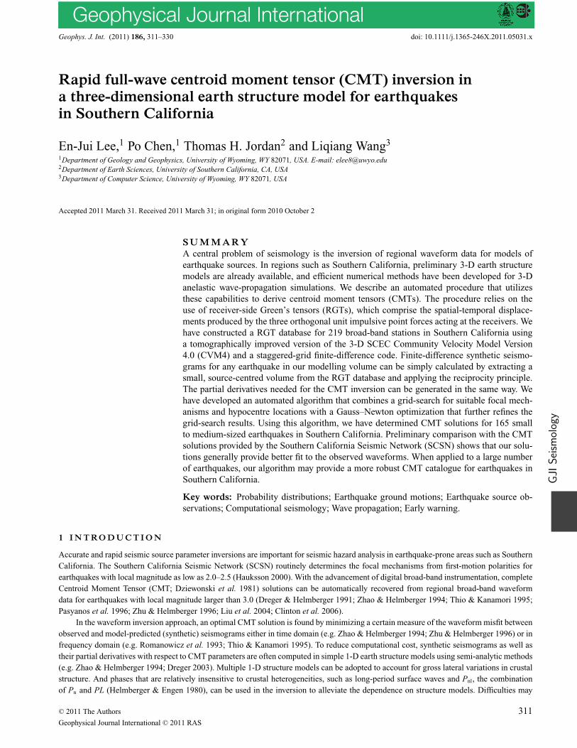
We illustrate our inversion procedure using the 2002 September 3 Mw 4.3 Yorba Linda earthquake as an example. The epicentre, the best-fittingdouble couple and the complete CMT solutions for this earthquake are shown in Fig. 4(a).

We retrieve broad-band, three-component seismic waveform data from the Southern California Earthquake Data Center. Two criteriawere used to reject seismograms with low SNR,

SNRA = AS/AN , (40)

where AN and AS are the maximum amplitudes before and after the first-arrival time, and

SNRE = ES/EN =∫ t1

S

t0S

u2(t)dt/(t1S − t0

S )

/∫ t1N

t0N

u2(t)dt/(t1N − t0

N ), (41)

where u(t) is the observed seismogram, [t0N , t1

N ] and [t0S , t1

S ] are time windows before and after the first-arrival time. In this study, we rejectedseismograms with SNRA or SNRE below five. The two horizontal components were rotated into radial and transverse components. We thenremove the mean and any linear trend in the seismogram and apply a sixth-order low-pass Butterworth filter with corner frequency at 0.2 Hz.For the 165 earthquakes analysed in this study, the number of seismograms with acceptable SNR ranges from 20 for an ML 3.16 earthquake to460 for the Mw 5.4 Chino Hills earthquake. In general, earthquakes with larger magnitudes usually have more high-quality data seismograms.

The filtered seismogram was then processed using an automated waveform segmentation algorithm to extract waveforms of our interest.Examples of the selected waveforms for the Yorba Linda earthquake are shown in Fig. 4(b). For the CMT inversions in this study, we primarilyextracted and fitted the first-arriving P- and S-waves and the surface waves on the observed seismograms. Our waveform segmentation andselection algorithm is based on the continuous wavelet transform, which allows us to detect and separate different wave groups with intersectingtemporal and/or frequency supports. The segmented seismograms are processed using an artificial neural network that is embedded withhuman knowledge about characteristics of certain seismic wave arrivals to automatically select a set of waveforms of our interest. The samealgorithm is also being used in our tomographic inversions. The details of our waveform segmentation and selection algorithm are documentedin a separate paper (Diersen et al. 2011).

The grid search as formulated in Section 2.2 is then carried out using the selected data waveforms. Throughout the three grid-searchstages, the source-model sample space is successively refined around the optimal solutions obtained from the previous stage. The samplinginterval reduces from 30◦ grid-spacing in strike, dip, rake and 2-km spacing in hypocentre locations in the first stage to 5◦ grid-spacing instrike, dip, rake and 0.5-km spacing in hypocentre locations in the last stage. The source-model subspace selected for refinement is controlledby P1 and P2 as defined in eqs (19) and (27). In our procedure, we found in general that P1 = 0.7 and P2 = 0.8 provide a good balancebetween search efficiency and solution accuracy. Throughout the grid-search step, thresholds Q0, Q1 and Q2, as defined in eqs (17), (25) and(34), are used to reject problematic data waveforms. If the probability for an individual measurement is below the threshold, it suggests thatthe particular data waveform cannot be fit well by any source solutions in the model sample space, which may due to instrumental problemsor unusually high noise level. In our procedure, we found that a value of 0.2 for these three thresholds provide a good balance betweensolution accuracy and algorithm robustness. The posterior probability density after the third grid-search stage is a 6-D function. The marginalprobability densities for strike, dip, rake and depth are plotted in Fig. 4(c).

The optimal solution obtained from the grid-search step is used as the initial solution in an iterative Gauss–Newton optimization asformulated in Section 2.3 and in Zhao et al. (2006) to find the optimal coefficients for the six basis moment tensors am (m = 1, 2, . . . 6).The partial derivatives of the GSDF measurements with respect to am are computed using eqs (38) and (39) and the Gauss–Newton normalequation is solved using the LSQR method (Paige & Saunders 1982). The perturbation obtained in the Gauss–Newton optimization stepis quite small, which is due to the fact that the grid search has been carried out through successively refined sample space. The isotropiccomponent of the complete moment tensor is constrained to be zero by setting a6 = 0 in our inversion. For the deviatoric part, we measurethe contribution of the non-double-couple component using the parameter ε = −λ2/ max(|λ1| , |λ3|), λ1, λ2 and λ3 being the eigenvalues ofthe moment tensor with λ1 ≥ λ2 ≥ λ3 (eq. 1 in Giardini 1983). For the Yorba Linda earthquake ε is less than 4 per cent and the best-fitting

C© 2011 The Authors, GJI, 186, 311–330



34˚

36˚

(a)

(b)

(c)

SRN

CPPWLT

PLS

MLS

BRE

STG

RIO

LLS

LTP

WTT

CHFSBPX

BBS

ADO

PLC

FRD

DPP

CCC

0 60 120 180 240 300 360

Strike (o)

0 15 30 45 60 75 90

Dip (o)

0 30 60 90

Rake (o)

4 8 12 16 20

Depth (km)

Transverse Radial VerticalNet.StaAz/DistCI.SRN187/ 10

CI.CPP349/ 16

CI.WLT302/ 19

CI.PLS131/ 21

CI.MLS64/ 22

CI.BRE237/ 23

CI.STG179/ 28

CI.RIO318/ 28

CI.LLS211/ 30

CI.LTP264/ 37

CI.WTT275/ 44

CI.CHF334/ 52

CI.SBPX55/ 61

CI.BBS89/ 74

CI.ADO24/ 77

CI.PLC95/117

AZ.FRD113/118

CI.DPP142/128

CI.CCC12/182

100 sec.

Figure 4. An example of our CMT inversion procedure. (a) The map shows epicentre of the 2002 September 3 Mw 4.3 Yorba Linda earthquake (the star) andthe best-fitting double couple solution (left beachball) and the full moment tensor solution (right beachball). Stations that have waveforms being selected forour inversion are shown as grey triangles. (b) Examples of the waveforms selected for our CMT inversion using our automated seismogram segmentation andselection algorithm. The black lines are observed seismograms and the red lines are synthetic seismograms computed using our optimal best-fitting doublecouple solution. The black bars below the seismograms indicate the waveforms we have selected for CMT inversion. (c) The marginal probability densities forstrike, dip, rake and depth obtained after our grid-search step.

double couple solution is plotted in Fig. 4(a). In general, for the 165 earthquakes analysed in this study, the value of ε is less than 10 per centand the best-fitting double couple solutions are shown in the figures.

Depending on the total number of data waveforms used in the inversion, it takes from around 30 s to about few minutes to complete thethree stages of grid search on 128 computing cores of the Intrepid (IBM Blue Gene/P) supercomputer at the Argonne Leadership ComputingFacility (ALCF). The computational cost for the Gauss–Newton optimization step is negligible compared with that for the grid-search stepand it usually takes one computing core less than 5 s for the LSQR algorithm to converge. The disk storage cost is substantial. The RGTsfor the 219 stations used in our CMT inversion and also in our full –3-D, full-wave tomographic inversion for Southern California currentlyoccupies around 400 TB (1 TB = 1024 GB) disk space on Intrepid.

C© 2011 The Authors, GJI, 186, 311–330



5 R E S U LT S

The SCSN automatically generate and catalogue moment tensor solutions and moment magnitudes for regional earthquakes with localmagnitude ML > 3.0 (Clinton et al. 2006). This automated algorithm inverts three-component, broad-band waveforms with period from 10 sto 100 s from at least four stations using pre-determined Green’s functions for various 1-D seismic velocity profiles calibrated for differentregions in Southern California. It can provide reliable moment tensor solutions for local events with ML > 4.0.

We have successfully applied our automated CMT inversion algorithm to 165 earthquakes with local magnitude 3.0 ≤ ML ≤ 5.7 inSouthern California. In general our CMT solutions are consistent with the SCSN automatically generated solutions and our solutions providebetter or equally good fit to the observed waveforms for frequencies up to 0.2 Hz. A comparison between the focal mechanisms we havedetermined with those from the SCSN moment tensor catalogue is shown in Fig. 1. Finite-difference synthetic seismograms were computedusing SCSN moment tensor solutions and our own CMT solutions in the same 3-D earth structure model, CVM4SI2. To quantify waveformmisfits within a certain time window [t0, t1], we use the following normalized misfit measure

F =∫ t1

t0

dt [u(t) − u(t)]2

/√∫ t1

t0

dt [u(t)]2

∫ t1

t0

dt [u(t)]2, (42)

where u(t) is the observed seismogram and u(t) is the corresponding synthetic seismogram (Zhu & Helmberger 1996). The advantage ofthis misfit definition is that it prevents a few strongest waveforms from dominating the misfit measure. The Pnl waves usually have smalleramplitudes than surface waves and stations close to the source usually have larger amplitudes. The normalization in eq. (42) helps to weightwaveforms with different amplitudes equally. We note that this misfit measure is only used for evaluating CMT solutions and it is not used inour inversion algorithm. Waveform misfits are quantified using normalized cross-correlation coefficients, cross-correlation traveltime shiftsand amplitude anomalies in our grid-search step and using frequency-dependent GSDF measurements in our Gauss–Newton optimizationstep. The justifications for not using eq. (42) in our CMT inversion algorithm are discussed in more detail in Section 6.

For the 165 earthquakes analysed in this study, the accumulative waveform misfit (i.e. the summation of F for all selected waveformsand all earthquakes) between the observed seismograms and the synthetics computed using our own CMT solutions is about 86 per cent of theaccumulative waveform misfit between observed seismograms and the synthetics computed using SCSN moment tensors. In this comparison,the synthetic seismograms for our own CMT solutions and for SCSN solutions are both computed using CVM4SI2 and the finite-differencemethod. We note that the forward modelling apparatus used for the comparison is identical to the one used in our CMT inversion, thereforeit could produce comparison results favouring our CMT solutions. Ideally, such a comparison should be carried out using an independentforward modelling apparatus with the true earth structure model, which is difficult, if possible at all, in practice. However, we think that ingeneral the 3-D CVM4SI2 provides better predictions of observed waveforms than the laterally homogeneous SoCaL model (e.g. Fig. 3)and might be closer to the actual structure model in general. At the current stage, CVM4SI2 is still being refined through our full-wavetomographic inversions. A more objective comparison could be conducted using an improved version of our tomographically refined 3-Dearth structure model, which will be documented in a future publication.

3 3.5 4 4.5 5 5.5 60

0.1

0.2

0.3

0.4

0.5

0.6

Mw

e

Figure 5. The difference in the normalized moment tensor e (eq. 43) as a function of earthquake moment magnitude. The magnitude interval from 3.0 to 6.0is separated evenly into six bins. The median of e for earthquakes in each bin is plotted at the centre of each magnitude bin. The peak between magnitudeinterval from 4.0 to 4.5 may be due to the fact that a number of earthquakes close to the north of Mexico have larger e (Fig. 7).

C© 2011 The Authors, GJI, 186, 311–330



34˚

35˚

SCEC3DDGR

OLI

CPP

LKL

PDUSBPX

SRN

SVD

VCS

RVR

CHNRUS

USCTHX

LFP

ID: 9659437

0

10

20

Num

ber

of S

eis

mogra

ms

0 2 4 6 8 10 12 14

Waveform misfit


CVM 1.43 2.12

SCSN 2.76 3.62

0 20 40

0 20 40

0 20 40

0 20 40

Time (s)

0 20 40

0 20 40

0 20 40

0 20 40

0 20 40

0 20 40

Time (s)

0 20 40

20 40

20 40 60

20 40 60 80

20 40 60 80

Time (s)

Figure 6. Waveform comparison for a small earthquake used in our study. Red beachball, focal mechanism determined using our CMT inversion algorithm;blue beachball, SCSN focal mechanism. Star, epicentre of the earthquake; blue triangles, station locations of waveform comparison examples. Black solid lines,observed seismograms; red solid lines, synthetic seismograms computed using our optimal CMT solution; blue solid lines, synthetic seismograms computedusing SCSN CMT solution. In the box, the histograms show the distributions of waveform misfits of SCSN CMT solution (grey area) and our optimal solution(area included by red line).

C© 2011 The Authors, GJI, 186, 311–330



Among the 165 earthquakes we have studied, a few of them have larger discrepancies with the SCSN moment tensor solutions. Ingeneral, the discrepancies are larger for smaller earthquakes and for earthquakes located close to the boundary of the seismic network. Wegive a more detailed explanation in the following.

5.1 CMT solutions for small earthquakes

As shown in Fig. 1, for the 165 earthquakes we have analysed so far, the CMT solutions determined using our method are generally consistentwith the SCSN solutions. To quantify the differences between our focal mechanisms and SCSN solutions, we define the quantity

e = (Mcvm − Mscsn) : (Mcvm − Mscsn), (43)

where Mcvm and Mscsn are normalized moment tensors for our focal mechanism and for the SCSN solution. We separate the magnitude rangeinto six bins with 0.5 magnitude interval. The median of e for earthquakes in each bin is shown in Fig. 5. In general, the difference in focalmechanism between our solution and the SCSN solution is larger at smaller magnitudes.

The smallest earthquake we have analysed so far has local magnitude ML = 3.16 (SCSN event ID 9659437). For this small earthquake,the SCSN automatic algorithm inverted waveforms at four stations and its solution is shown in Fig. 6. Due to the small magnitude of thisearthquake, the signal-to-noise ratio of observed waveforms with period longer than 10 s is quite low, which partly explains the low variancereduction (7.52 per cent) obtained by the SCSN algorithm. To improve the signal-to-noise ratio of the observed waveforms, we need to reducethe shortest period to below 10 s. The 3-D seismic velocity model CVM4SI2 used in our algorithm can provide accurate Green’s functionsfor frequencies up to 0.2 Hz, which allows us to fit observed waveforms at 5 s or longer. For this small earthquake, the centroid locationdetermined using our algorithm is about 3 km shallower than the SCSN solution and the difference in dip is about 20◦ (Fig. 6). Comparisonwith the observed waveforms low-pass filtered to 0.2 Hz shows that the synthetics generated using our CMT solution provide better fit thanthose generated using the SCSN solution (Fig. 6). We note that the improvements in the waveform fits are caused by differences in thesource parameters only. The structure model and the forward modelling apparatus for computing synthetics are identical. For this earthquake,the shallower centroid location in our CMT solution causes different excitations of surface waves, which may explain the better fits to theobserved surface waves.

For the 10 smallest earthquakes (3.11 ≤ Mw ≤ 3.51) analysed in this study, the ratio between the accumulative misfit for our solution andthe accumulative misfit for SCSN solution ranges from around 0.44 to around 0.95, which suggests that our solutions fit observed waveformsbetter than SCSN solutions or equally well in general. By using a well-calibrated 3-D seismic structure model to generate Green’s functions,our synthetics can fit observed waveforms at higher frequencies than synthetics generated using 1-D models, thereby providing more robustCMT solutions for earthquakes with smaller magnitudes.

5.2 Effects of station azimuthal coverage

Among the earthquakes with relatively large discrepancies between our CMT solutions and the SCSN solutions, many of them lie close tothe boundary of the seismic network (Fig. 7), in which case the station azimuthal coverage can be poor. An example is shown in Fig. 8. Forthis ML 4.33 earthquake (SCSN event ID 14178236), the difference in centroid location between our solution and the SCSN solution is lessthan 1 km, the difference in focal mechanism is significant (Fig. 8). Synthetics generated using our CMT solution generally provide betterfit to the observed waveforms, especially for longer source-station paths that traverse basins (Fig. 8). The 1-D seismic structure model usedfor determining the SCSN solution might not provide good approximations for those source-station paths, which introduces a bias into theestimated CMT solution. Such a bias due to inaccuracy in seismic structure model is alleviated when the azimuthal coverage of the seismicstations is good.

5.3 Depths of earthquakes

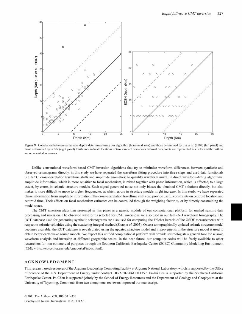
The RGT database and the reciprocity principle allow us to conduct efficient grid search to find the optimal epicentre locations and depthsof earthquakes without running additional wave-propagation simulations. The grid spacing of our RGT database is 500 m, which gives us aspatial resolution up to 250 m in earthquake depth during the grid-search step.

For the 165 earthquakes analysed in this study, their depths range from around 2 km to about 18 km. The amplitudes of the surfacewaves used in the inversion give us strong constraints on earthquake depths. A comparison of the earthquake depths determined using ourown algorithm and those determined by Lin et al. (2007a) using a 3-D seismic structure model (Lin et al. 2007b) and those extracted fromthe SCSN moment tensor catalogue is shown in Fig. 9. In general, the depths determined using our own algorithm correlates well withthose determined by Lin et al. (2007a). For the outliers in Fig. 9(a), we conducted a grid search at the earthquake locations provided by Linet al. (2007a) and generated synthetic seismograms for the optimal focal mechanisms. We found that in general, synthetics generated usingour CMT solutions provide better fit to surface-wave amplitudes than those generated using the optimal focal mechanisms at the locationsprovided by Lin et al. (2007a). An example is shown in Fig. 10 for a magnitude about 4.98 earthquake (SCSN event ID 14065544) in theoffshore region. For this earthquake, the depth provided by Lin et al. (2007a) is 33.97 km and the depth provided by our algorithm is about13.5 km. Synthetics computed using our CMT solution provide much better fit to the observed waveforms, especially for the surfaces waves.

C© 2011 The Authors, GJI, 186, 311–330



32˚

34˚

36˚

38˚

Mw <4.0 4~4.5 >4.5e 0.1 1.0 2.0

Figure 7. Geographic distribution of the difference in normalized moment tensor e (eq. 43). The radii of the circles are proportional to the size of e and thecentres of the circles are located at the epicentre locations of the analysed earthquakes. The colour of the circle is corresponding to the moment magnituderange of the earthquake.

Synthetics generated using the location provided by Lin et al. (2007a) generally do not have sufficient amplitudes for the surface waves,which suggests that Lin et al. (2007a) may have overestimated the depth of this earthquake.

5.4 Moment magnitudes of earthquakes

For most of the earthquakes analysed in this study, the moment magnitudes provided by our algorithm are in good agreement with thoseprovided by the SCSN moment tensor catalogue, except for a few outliers (Fig. 11a). The same outliers also exist on the correlation plotbetween the SCSN ML and SCSN Mw (Fig. 11b). The correlation plot between our Mw estimates and SCSN ML estimates (Fig. 11c) has largerscattering than that between our Mw estimates and SCSN Mw estimates. However, for the outliers in Fig. 11(a) and (b), our Mw estimatesseem to correlate better with the SCSN ML estimates than the SCSN Mw estimates, which suggests that the SCSN automated algorithm mayhave overestimated the moment magnitudes of those earthquakes.

6 D I S C U S S I O N

In this study, we have extended the CMT inversion algorithm based on the RGT database introduced in Zhao et al. (2006) to includea grid-search step. The formulation presented in this paper allows us not only to obtain an optimal solution but also to quantify uncer-tainties in the solution. The procedure allows us to iteratively condition the model space by rejecting solutions with low probabilities. Atthe beginning of step 2 in our grid-search procedure, by selecting appropriate values for the probability threshold P1, we can reject solu-tions that do not provide sufficiently high NCC values, thereby ensuring the accuracy of the cross-correlation traveltime shifts measuredin step 2 and the amplitude anomalies measured in step 3. The sample space and the sampling intervals are successively refined onlyaround regions in the model space that have higher probabilities and high accuracy in the solution is achieved with minimal computingtime.

C© 2011 The Authors, GJI, 186, 311–330



33˚

34˚

35˚

SCEC3DGLA

BZN

ALP

ARV

BBR

DEV

ERR

FMP

DSC

ADO

DPP

SES

ID: 14178236

0

20

40

60

80

100

Num

ber

of S

eis

mogra

ms

0 2 4 6 8 10 12 14

Waveform misfit


CVM 1.09 1.60

SCSN 1.89 2.42

0 20 40

20 40 60

20 40 60

20 40 60

Time (s)

40 60 80 100

20 40 60 80

40 60 80 100

40 60 80 100

Time (s)

60 80 100 120

80 100 120 140

100 120 140 160

100 120 140 160

Time (s)

Figure 8. Waveform comparison for an earthquake with relatively poor azimuthal station coverage. Red beachball, focal mechanism determined using ourCMT inversion algorithm; blue beachball, SCSN focal mechanism. Star, epicentre of the earthquake; blue triangles, station locations of waveform comparisonexamples. Black solid lines, observed seismograms; red solid lines, synthetic seismograms computed using our optimal CMT solution; blue solid lines, syntheticseismograms computed using SCSN CMT solution. In the box, the histograms show the distributions of waveform misfits of SCSN CMT solution (grey area)and our optimal solution (area included by red line).

C© 2011 The Authors, GJI, 186, 311–330



0 5 10 15 20 250

5

10

15

20

25

30

35

Depth (Km)

De

pth

(K

m ; L

in e

t a

l.,

20

07

)

0 5 10 15 20 250

5

10

15

20

25

Depth (Km)

SC

SN

Depth

(K

m)

Figure 9. Correlation between earthquake depths determined using our algorithm (horizontal axes) and those determined by Lin et al. (2007) (left panel) andthose determined by SCSN (right panel). Dash lines indicate locations of two standard deviations. Normal data points are represented as circles and the outliersare represented as crosses.

Unlike conventional waveform-based CMT inversion algorithms that try to minimize waveform differences between synthetic andobserved seismograms directly, in this study we have separated the waveform fitting procedure into three steps and used data functionals(i.e. NCC, cross-correlation traveltime shifts and amplitude anomalies) to quantify waveform misfit. In direct waveform-fitting algorithms,amplitude information, which is more sensitive to focal mechanism, is mixed together with phase information, which is affected, to a largeextent, by errors in seismic structure models. Such signal-generated noise not only biases the obtained CMT solutions directly, but alsomakes it more difficult to move to higher frequencies, at which errors in structure models might increase. In this study, we have separatedphase information from amplitude information. The cross-correlation traveltime shifts can provide useful constraints on centroid location andcentroid time. Their effects on focal mechanism estimates can be controlled through the weighting factor μn or by directly constraining themodel space.

The CMT inversion algorithm presented in this paper is a generic module of our computational platform for unified seismic dataprocessing and inversion. The observed waveforms selected for CMT inversions are also used in our full –3-D waveform tomography. TheRGT database used for generating synthetic seismograms are also used for computing the Frechet kernels of the GSDF measurements withrespect to seismic velocities using the scattering-integral method (Zhao et al. 2005). Once a tomographically updated seismic structure modelbecomes available, the RGT database is re-calculated using the updated structure model and improvements in the structure model is used toobtain better earthquake source models. We expect this unified computational platform will provide seismologists a general tool for seismicwaveform analysis and inversion at different geographic scales. In the near future, our computer codes will be freely available to otherresearchers for non-commercial purposes through the Southern California Earthquake Center (SCEC) Community Modelling Environment(CME) (http://epicenter.usc.edu/cmeportal/index.html).

A C K N OW L E D G M E N T

This research used resources of the Argonne Leadership Computing Facility at Argonne National Laboratory, which is supported by the Officeof Science of the U.S. Department of Energy under contract DE-AC02–06CH11357. En-Jui Lee is supported by the Southern CaliforniaEarthquake Center. Po Chen is supported jointly by the School of Energy Resources and the Department of Geology and Geophysics at theUniversity of Wyoming. Comments from two anonymous reviewers improved our manuscript.

C© 2011 The Authors, GJI, 186, 311–330



33˚

34˚

35˚

14065544

BZN

ADOALP

BBR

CCC

DSC

GLA

TEH

CIA

SRN

GOR

TOV

0

20

40

60

80

100

120

140

Nu

mb

er

of

se

ism

og

ram

s

0 2 4 6 8 10 12 14

Waveform misfit


3D 1.40 1.81

DD 2.78 3.63

20 40 60

20 40 60

40 60 80

40 60 80

Time (s)

40 60 80 100

40 60 80 100

40 60 80 100

60 80 100 120

Time (s)

60 80 100 120 140

60 80 100 120 140

60 80 100 120 140

60 80 100 120 140

Time (s)

Figure 10. Comparison of waveforms for a magnitude about 4.98 offshore earthquake. Synthetics were generated using the CMT solution determined by ouralgorithm at our optimal location (red star) and at the location (blue star) provided by Lin et al. (2007a). Black solid lines, observed seismograms; red solid lines,synthetic seismograms computed using our optimal CMT solution and location (depth = 13.5 km); blue solid lines, synthetic seismograms computed using ouroptimal CMT solution at location (depth = 34 km) in Lin et al.’s (2007a) catalogue; blue triangles, station locations of waveform comparison examples. In thebox, the histograms show the distributions of waveform misfits at Lin et al.’s (2007a) location (grey area) and our optimal solution (area included by red line).

C© 2011 The Authors, GJI, 186, 311–330



Figure 11. (a) Correlation between the Mw determined using our algorithm with the Mw determined by SCSN for earthquakes analysed in this study, normaldata points are represented as circles and the outliers are represented as crosses; (b) correlation between SCSN Mw and SCSN ML; (c) correlation between ourMw estimates and SCSN ML for the same set of earthquakes. The dash lines in (a) indicate location of two standard deviations. We note that the same outliers(crosses) in (a) are also plotted as crosses in (b) and (c).

R E F E R E N C E S

Akcelik, V. et al., 2003. High-resolution forward and inverse earthquakemodeling on terascale computers, in Proceedings of the ACM/IEEESupercomputing SC’2003 Conference, Phoenix, AZ.

Aki, K. & Richards, P.G., 2002. Quantitative Seismology, 2nd edn, Univer-sity Science Books, Sausalito, CA.

Chen, P., Zhao, L. & Jordan, T.H., 2007. Full 3D tomography for crustalstructure of the Los Angeles region, Bull. seism. Soc. Am., 97, 1094–1120.

Chen, P., Jordan, T.H. & Lee, E., 2010. Perturbation kernels for generalizedseismological data functionals (GSDF), Geophys. J. Int., 183, 869–883,doi:10.1111/j.1365-246X.2010.04758.x

Clinton, J.F., Hauksson, E. & Solanki, K., 2006. An evaluation of the SCSNmoment tensor solutions: robustness of the Mw magnitude scale, styleof faulting, and automation of the method. Bull. seism. Soc. Am., 96(5),1689–1705, doi:10.1785/0120050241.

Diersen, S., Lee, E., Spears, D., Chen, P. & Wang, L., 2011. Classification of

seismic windows using artificial neural networks. in Proceedings of the11th International Conference on Computer Science, Tsukuba, Japan.

Dreger, D.S., 2003. TDMT_INV: time domain seismic moment tensor IN-Version, in International Handbook of Earthquake and Engineering Seis-mology, Vol. 81B, p. 1627, Academic Press, San Diego, CA.

Dreger, D.S. & Helmberger, D., 1991. Source parameters of the Sierra Madreearthquake from regional and local body waves, Geophys. Res. Lett., 18,2015–2018.

Dreger, D.S. & Helmberger, D.V., 1993. Determination of source parame-ters at regional distances with three-component sparse network data, J.geophys. Res., 98, 8107–8125.

Dziewonski, A.M., Chou, T.-A. & Woodhouse, J. H., 1981. Determinationof earthquake source parameters from waveform data for studies of globaland regional seismicity, J. geophys. Res. 86, 2825–2852

Fichtner, A., Kennett, B.L.N., Igel, H., Bunge, H.-P., 2009. Full seismicwaveform tomography for upper-mantle structure in the Australasian re-gion using adjoint methods, Geophys. J. Int., 179, 1703–1725.

C© 2011 The Authors, GJI, 186, 311–330



Fichtner, A., Kennett, B.L.N., Igel, H., Bunge, H.-P., 2010. Full waveformtomography for radially anisotropic structure: new insights into presentand past states of the Australasian upper mantle. Earth planet. Sci. Lett.,290, 270–280.

Gee, L.S. & Jordan, T.H., 1992. Generalized seismological data functionals,Geophys. J. Int., 111, 363–390.

Giardini, D., 1983. Regional deviation of earthquake source mechanismsfrom the ‘double-couple’ model, in Earthquakes: Theory and Interpreta-tion, pp. 345–353, eds. Kanmori, H. & Bosch, E., North-Holland, Ams-terdam.

Graves, R., 1996. Simulating seismic wave propagation in 3D elastic me-dia using staggered-grid finite differences, Bull. seism. Soc. Am., 86,1091–1106.

Hadley, D. & Kanamori, H., 1977. Seismic structure of the TransverseRanges, California, Geol. Soc. Am. Bull., 88, 1469–1478.

Hardebeck, J.L. & Shearer, P.M., 2002. A new method for determiningfirst-motion focal mechanisms, Bull. seism. Soc. Am., 92, 2264–2276.

Hauksson, E., 2000. Crustal structure and seismicity distribution adjacentvtothe Pacific and North America plate boundary in southern California, J.geophys. Res., 105, 13 875–13 903.

Helmberger, D.V. & Engen, G.R., 1980. Modeling the long-period bodywaves from shallow earthquakes at regional ranges, Bull. seism. Soc. Am.,70, 1699–1714.

Hingee, M., Tkalcic, H., Fichtner, A. & Sambridge, M., 2010. Seis-mic moment tensor inversion using a 3-D structural model: appli-cations for the Australian region. Geophys. J. Int., 184, 949–964,doi:10.1111/j.1365–246X.2010.04897.x.

Kikuchi, M. & Kanamori, H., 1991. Inversion of complex body waves—III,Bull. seism. Soc. Am. 81, 2335–2350.

Kohler, M.D., Magistrale, H. & Clayton, R.W., 2003. Mantle heterogeneitiesand the SCEC reference three-dimensional seismic velocity model ver-sion 3, Bull. seism. Soc. Am., 93, 757–774.

Komatitsch, D., Liu, Q., Tromp, J., Suss, P., Stidham, C. & Shaw, J.H.,2004. Simulations of ground motion in the Los Angeles basin based uponspectral-element method, Bull. seism. Soc. Am., 94, 187– 206.

Lin, G., Shearer, P.M. & Hauksson, E., 2007a. Applying a three-dimensionalvelocity model, waveform cross correlation, and cluster analysis to locatesouthern California seismicity from 1981 to 2005, J. geophys. Res., 112,B12309, doi:10.1029/2007JB004986

Lin, G., Shearer, P.M., Hauksson, E. & Thurber, C.H., 2007b. A three-dimensional crustal seismic velocity model for southern Californiafrom a composite event method. J. geophys. Res., 112, B11306,doi:10.1029/2007JB004977.

Liu, Q.-Y., Polet, J., Komatitcsh, D. & Tromp, J., 2004. Spectral-elementmoment tensor inversions for earthquakes in Southern California, Bull.seism. Soc. Am., 94, 1748–1761.

Ma, S., Prieto, G.A. & Beroza, G.C., 2008. Testing community velocitymodels for southern California using the ambient seismic field, Bull.seism. Soc. Am., 98, 2694–2714.

Magistrale, H., Day, S., Clayton, R.W. & Graves, R., 2000. The SCECSouthern California reference three-dimensional seismic velocity modelVersion 2, Bull. seism. Soc. Am., 90, S65–S76.

Okamoto, T., 1994a. Location of shallow subduction zone earthquake

inferred from teleseismic body waveform, Bull. seism. Soc. Am., 84,264–268.

Okamoto, T., 1994b. Teleseismic synthetics obtained from 3-D calculationsin 2-D media, Geophys. J. Int., 118, 613–622.

Okamoto, T., 2002. Full waveform moment tensor inversion by reciprocalfinite difference Green’s function, Earth Planets Space, 54, 715–720.

Olsen, K.B., 1994. Simulation of three-dimensional wave propagation in theSalt Lake Basin, PhD thesis. University of Utah, Salt Lake City, 157 pp.

Olsen, K.B., Day, S.M. & Bradley, C.R., 2003. Estimation of Q for long-period (>2 s) waves in the Los Angeles Basin, Bull. seism. Soc. Am., 93,627–638.

Paige, C. & Saunders, M., 1982. Algorithm 583 LSQR: sparse linearequations and least squares problems, ACM Trans. Math. Softw., 8(2),195–209.

Pasyanos, M.E., Dreger, D.S. & Romanowicz, B., 1996. Towards real-timedetermination of regional moment tensors, Bull. seism. Soc. Am., 86,1255–1269.

Ramos-Martınez, J. & McMechan, G.A., 2001. Source-parameter estimationby full waveform inversion in 3D heterogeneous, viscoelastic, anisotropicmedia, Bull. seism. Soc. Am., 91, 276–291.

Ritsema, J., Rivera, L., Komatitsch, D., Tromp, J. & van Heijst, H.J., 2002.The effects of crust and mantle heterogeneity on PP/P and SS/S amplituderatios, Geophys. Res. Lett., 29, doi:10.1029/2001GL013831.

Romanowicz, B., Dreger, D., Pasyanos, M. & Uhrhammer, R., 1993. Moni-toring of strain release in central and northern California using broadbanddata, Geophys. Res. Lett., 20, 1643–1646.

Shearer, P., Hauksson, E. & Lin, G., 2005. Southern California hypocenterrelocation with waveform cross-correlation, Part 2: results using source-specific station terms and cluster analysis, Bull. seism. Soc. Am., 95,904–915, doi:10.1785/0120040168.

Subramanian, V., Wang, L., Lee, E. & Chen, P., 2010. Rapid processing ofsynthetic seismograms using Windows azure cloud, in Proceedings of theIEEE CloudCom 2010, Indianapolis, IN.

Suss, M.P. & Shaw, J.H., 2003. P-wave seismic velocity structure derivedfrom sonic logs and industry reflection data in the Los An- geles basin,California, J. geophys. Res., 108, 2170, doi:10.1029/2001JB001628.

Thio, H.K. & Kanamori, H., 1995. Moment-tensor inversions for local earth-quakes using surface waves recorded at TERRAscope, Bull. seism. Soc.Am., 95, 1021–1038.

Zhao, L. & Helmberger, D.V., 1994. Source estimation from broadbandregional seismograms, Bull. seism. Soc. Am., 84, 91–104.

Zhao, L., Jordan, T.H., Olsen, K.B. & Chen, P., 2005. Frechet kernels forimaging regional earth structure based on three-dimensional referencemodels, Bull. seism. Soc. Am., 95, 2066–2080.

Zhao, L., Chen, P. & Jordan, T.H., 2006. Strain Green’s tensors, reciprocityand their applications to seismic source and structure studies, Bull. seism.Soc. Am., 96(5), 1753–1763.

Zhu, L. & Helmberger, D.V., 1996. Advancement in source estimation tech-niques using broadband regional seismograms, Bull. seism. Soc. Am., 86,1634–1641.

Zhu, L. & Kanamori, H., 2000. Moho depth variation in Southern Cal-ifornia from teleseismic receiver functions, J. geophys. Res., 105(B2),2969–2980.

C© 2011 The Authors, GJI, 186, 311–330


geophysical journal international - uwyo.edulwang7/papers/jgeophysical2011.pdf · 1department of...

Documents