geophysical modeling in vlbi - chalmers
TRANSCRIPT
D. S. MacMillan VLBI Training School March 2013
Geophysical Modeling in VLBI
Dan MacMillan NVI Inc./NASA GSFC
EGU and IVS Training School on VLBI for
Geodesy and Astrometry Aalto University, Espoo, Finland
March 2-5, 2013
D. S. MacMillan VLBI Training School March 2013
1. Calculation of the Theoretical Delay
2. Tide Generating Potential
3. Site Displacement Contributions to the Calculation of Theoretical Delay
a. Solid Earth Tides
b. Rotational Deformation due to Polar Motion (Pole Tide)
c. Ocean Pole Tide Loading d. Ocean Tidal Loading
e. Nontidal Loading (Atmosphere, Hydrology, Ocean)
f. Other Models (antenna thermal deformation)
Overview
D. S. MacMillan VLBI Training School March 2013
Theoretical Delay
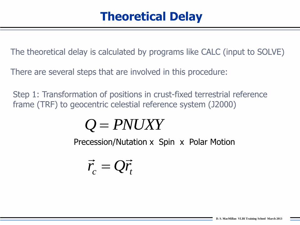
The theoretical delay is calculated by programs like CALC (input to SOLVE) There are several steps that are involved in this procedure:
Step 1: Transformation of positions in crust-fixed terrestrial reference frame (TRF) to geocentric celestial reference system (J2000)
PNUXYQ
tc rQr
Precession/Nutation x Spin x Polar Motion
D. S. MacMillan VLBI Training School March 2013
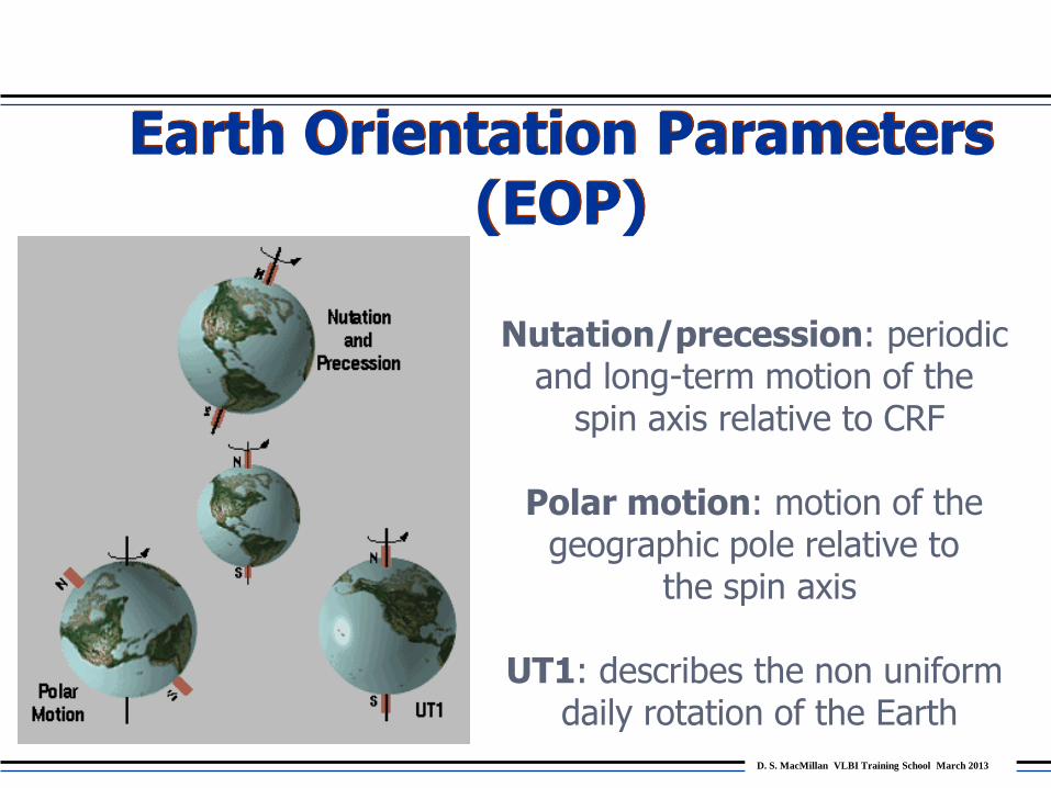
Earth Orientation Parameters (EOP)
Nutation/precession: periodic and long-term motion of the
spin axis relative to CRF
Polar motion: motion of the geographic pole relative to
the spin axis
UT1: describes the non uniform daily rotation of the Earth

D. S. MacMillan VLBI Training School March 2013
Theoretical Delay
Step 2. Compute Displacement Models and Delay Corrections for each site • Solid Earth (largest for 12 h band, up to 40 cm in vertical) • Ocean Loading (largest for 12 h band, mm-cm in vertical) • Pole Tide (12,14 months period, mm-cm) • Ocean Pole Tide Loading (mm) • [Atmosphere Pressure Loading] –{in Solve} • Site velocities – {in Solve}
Other Physical Offsets: • Axis offset correction (cm-m) • [Antenna thermal expansion/contraction (mm-cm)] –{in Solve} Refractive Media Delays: • Atmosphere delays (NMF) (nsecs) –{VMF in Solve} • [Ionosphere delays] (hundreds of psec) {X/S or GPS in Solve}
D. S. MacMillan VLBI Training School March 2013
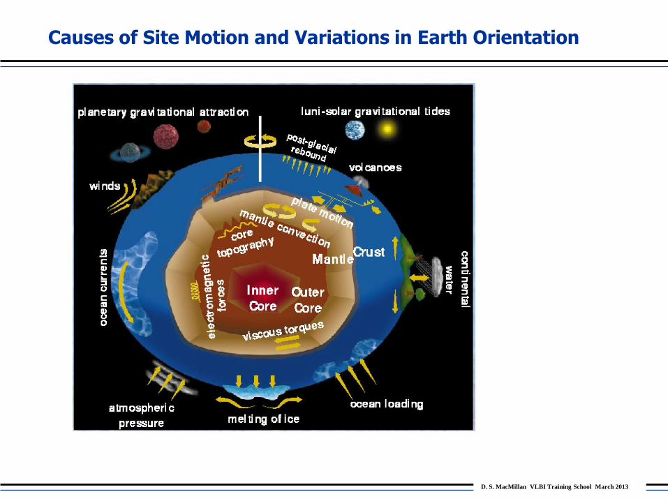
Causes of Site Motion and Variations in Earth Orientation
D. S. MacMillan VLBI Training School March 2013
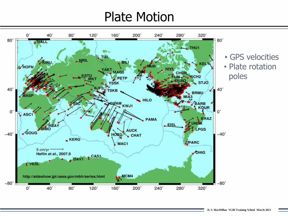
Plate Motion
• GPS velocities • Plate rotation poles
D. S. MacMillan VLBI Training School March 2013
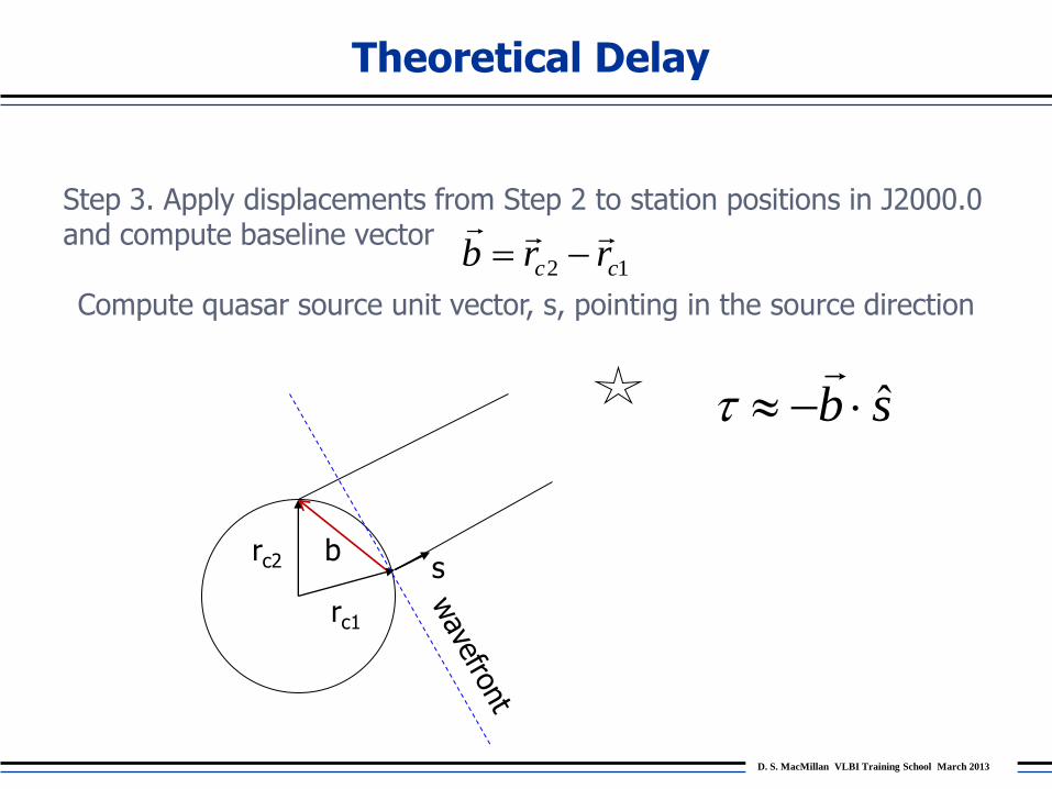
Theoretical Delay
Step 3. Apply displacements from Step 2 to station positions in J2000.0 and compute baseline vector
Compute quasar source unit vector, s, pointing in the source direction
12 cc rrb
rc1
rc2 b s
sb ˆ

D. S. MacMillan VLBI Training School March 2013
Theoretical Delay
Step 4. Compute Theoretical Delay • Use the Eubanks ‘Consensus’ Model. [see IERS Conventions 2010] • acccount for gravitational deflection from sun, moon, Earth, other planets. • Requires relativistic transformation to/from solar system barycentric coordinates • Add atmosphere geometric path delay contribution
D. S. MacMillan VLBI Training School March 2013
gTTXTXKc
TT )]()([1
112212
Vacuum delay in the solar system barycentric (SSB) frame
J
gJg TT
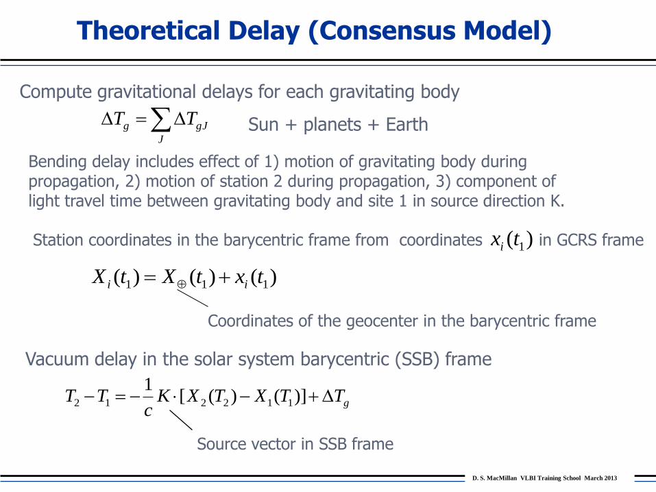
Bending delay includes effect of 1) motion of gravitating body during propagation, 2) motion of station 2 during propagation, 3) component of light travel time between gravitating body and site 1 in source direction K.
Compute gravitational delays for each gravitating body
Sun + planets + Earth
Theoretical Delay (Consensus Model)
)()()( 111 txtXtX ii
Station coordinates in the barycentric frame from coordinates in GCRS frame )( 1txi
Coordinates of the geocenter in the barycentric frame
Source vector in SSB frame
D. S. MacMillan VLBI Training School March 2013
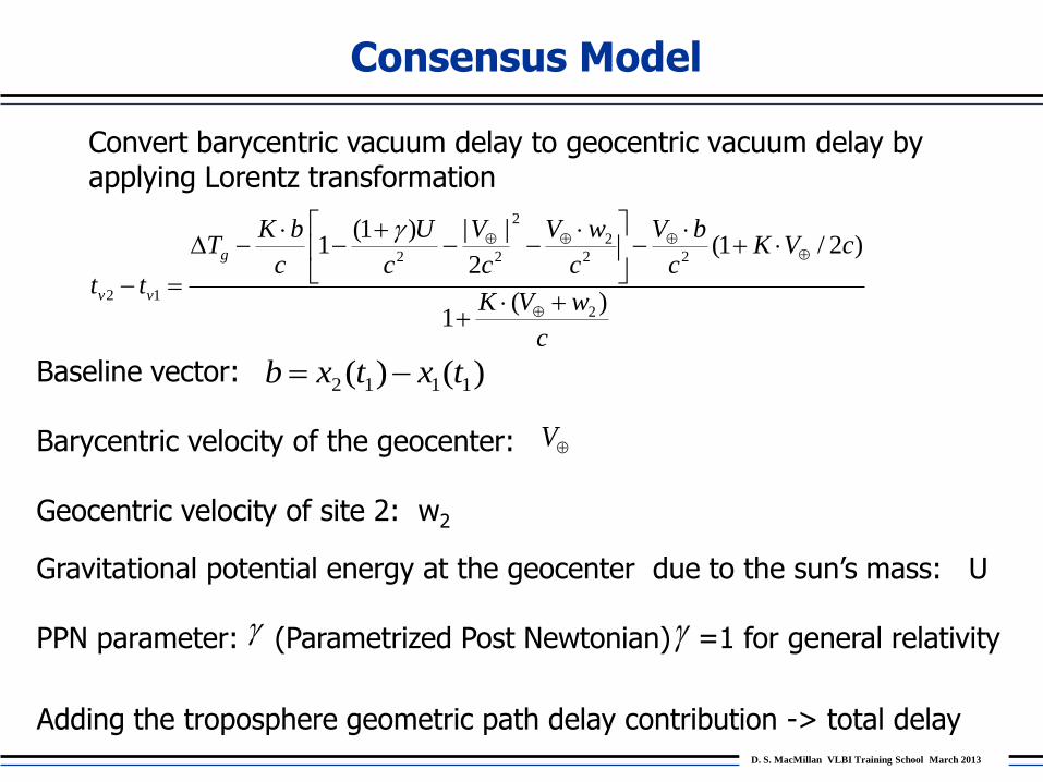
Convert barycentric vacuum delay to geocentric vacuum delay by applying Lorentz transformation
c
wVK
cVKc
bV
c
wV
c
V
c
U
c
bKT
tt
g
vv )(1
)2/1(2
||)1(1
2
22
2
2
22
12
Baseline vector: Barycentric velocity of the geocenter: Geocentric velocity of site 2: w2
Gravitational potential energy at the geocenter due to the sun’s mass: U PPN parameter: (Parametrized Post Newtonian) =1 for general relativity
)()( 1112 txtxb
V
Adding the troposphere geometric path delay contribution -> total delay
Consensus Model
D. S. MacMillan VLBI Training School March 2013
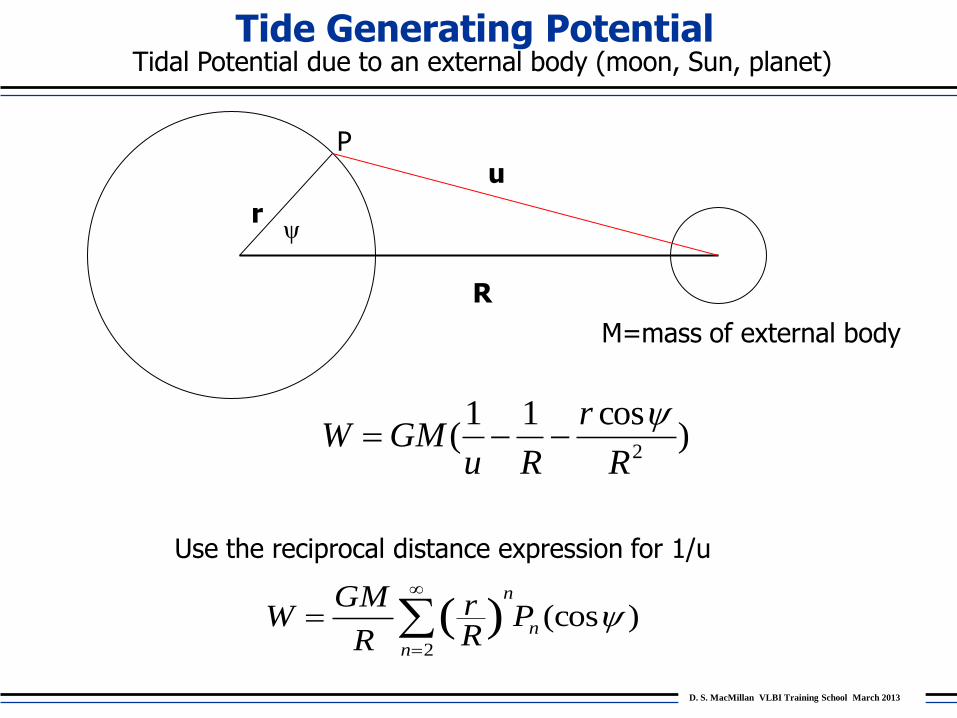
Tide Generating Potential Tidal Potential due to an external body (moon, Sun, planet)
)cos11
(2R
r
RuGMW
u
R
r ψ
)(cos2
)( n
n
n
PRr
R
GMW
P
Use the reciprocal distance expression for 1/u
M=mass of external body

D. S. MacMillan VLBI Training School March 2013
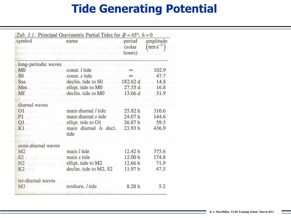
Tide Generating Potential
)(cos)( 2
2
2 PR
r
R
GMW
Main Tidal Potential:
Direction of lunar tidal-raising force: Only radial component at multiples of Transverse+radial at intermediate points
))2cos(31(2 3
R
MrGar
)2sin(32 3
R
MrGa
2/
2/

D. S. MacMillan VLBI Training School March 2013
Tide Generating Potential
Third-degree Potential:
)(cos3
3
3 PR
r
R
GMW
803
2
3
2
P
P
r
R
W
W
Relative strength of the lunar and solar tide-raising forces
2.2
3
moon
sun
sun
moon
S
L
R
R
M
M
a
a

D. S. MacMillan VLBI Training School March 2013
))]((cos[())((cos)(cos12
1)(
2 01
tmtPPnr
rGMtV bbnmnm
n
n
mn
b
n
b
Evaluate the potential using geocentric coordinates
of the (sun,moon,planets) )](),([ tt bb
Hartmann and Wenzel (1995) expand the TGP in terms of the Legendre functions of the ephemerides
Hartmann and Wenzel used JPL ephemerides DE200/LE200
Tide Generating Potential
(θ, λ, r) are the geocentric station coordinates
+ terms that account for the Earth’s flattening effect

D. S. MacMillan VLBI Training School March 2013
i
i
nm
ii
nm
n
m
nm
n
n
ttSttC
Pa
rtV
i))(sin()())(cos()(
)(cos)(0
6
1
11
1
)()(j
j
jiji tkmt
The full tidal potential was expressed by HW in terms of the following expansion by process of least-squares fitting and spectral analysis of residuals:
Functions of the astronomical arguments for each tide:
Truncated at n=6 (moon), n=3 (sun), n=2 (planets)
Tide Generating Potential
.
___
__
__
___
etc
perigeelunarlongitudemeanp
longitudesolarmeanh
longitudelunarmeans
timelunarlocalmean
Estimated 12935 coefficients nm
i
nm
i
nm
i CtCC 10
nm
i
nm
i
nm
i StSS 10
D. S. MacMillan VLBI Training School March 2013
Tide Generating Potential

D. S. MacMillan VLBI Training School March 2013
Solid Earth Tides
First compute in-phase displacements in the time domain, here for deg 2, but deg 3 is similar. - nominal (frequency independent) values for Love numbers (hn, ln) - avoids having to sum over very large number of terms of TGP above
Displacement from degree 2 TGP with nominal values for h2 and l2
]}ˆ)ˆˆ(ˆ)[ˆˆ(3]2
1)ˆˆ(
2
3[̂{ 2
23
2
22 rrRRrRlrRrhFr jjjj
j
j
3
4
jE
Ej
jRGM
RGMF
]ˆ,ˆcos
,ˆ[1
),,( nV
leVl
rVhg
neu nn
nnnnn
rR
rRPlrPhR
rr
M
Mr nnnn
n
E
n
ˆˆcos
}]ˆcosˆ){('ˆ)(cos[)( 1
jR
-Vector from geocenter to moon(j=2) or sun(j=3) -Earth radius ER
deg Moon Sun
2 425 mm 173 mm
3 7.5 mm 0.008 mm
4 0.13 mm 0.000 mm
)(cos),(2
)(
n
n
n
PRr
R
GMRrV
Love number response
D. S. MacMillan VLBI Training School March 2013
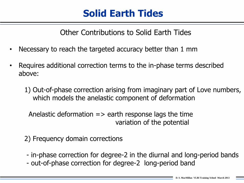
Solid Earth Tides
Other Contributions to Solid Earth Tides
• Necessary to reach the targeted accuracy better than 1 mm • Requires additional correction terms to the in-phase terms described
above: 1) Out-of-phase correction arising from imaginary part of Love numbers, which models the anelastic component of deformation Anelastic deformation => earth response lags the time variation of the potential 2) Frequency domain corrections
- in-phase correction for degree-2 in the diurnal and long-period bands - out-of-phase correction for degree-2 long-period band

D. S. MacMillan VLBI Training School March 2013
Rotational Deformation due to Polar Motion - Poletide
2222 ||2
1])([
2
1rrrVc
cc Va
rrrac
2)()(
The centrifugal potential corresponding to this acceleration is
)'('2' rvaa
Acceleration in the fixed frame, where
the primed system is rotating
Coriolis acceleration Centrifugal acceleration
Ωx(Ωxr’)
Ω
r’
O’

D. S. MacMillan VLBI Training School March 2013
Rotational Deformation due to Polar Motion - Poletide
Motion of the rotation axis about the geographic pole:
Radius ~ 10-12m

D. S. MacMillan VLBI Training School March 2013
]ˆ)1(ˆˆ[0 zmymxm zyx
Vg
hU 2 V
g
lE
sin
12 Vg
lN
2
)]sincos(2[sin2
1),( 22
0 yx mmrV
2222 ||2
1])([
2
1rrrV
Angular rotation of the Earth
Time-dependent offsets of pole Fractional variation in rotation rate
)()](22)([2
1 222222
0 mOymxmzmyxyxV yxz
Rotational Deformation due to Polar Motion - Poletide
Site displacement response to the potential via Love numbers:
0836.0,6207.0 22 lh
Average rotation rate
[Wahr, 1985]
mz variation ~ 1/100 mx or my

D. S. MacMillan VLBI Training School March 2013
Rotational Deformation due to Polar Motion - Poletide
)sincos(2sin33 yx mmU
)cossin(cos9 yx mmE
)sincos(2cos9 yx mmN
Mean pole IERS Conventions (2010): quadratic before 2010, linear after 2010
),( pp yx
ppx xxm ppy yym
in mm

D. S. MacMillan VLBI Training School March 2013
Additional potential due to external potential V U = k V H1 = (1+k)V/g Ocean surface (geoid) adjusts to this level. Height of the body tide. Deformation adjustment of solid earth height H2 = h V/g Resultant height of the ocean (measured relative to deformed solid earth) H = H1-H2 = (1+k-h)V/g k and h are Love numbers that give response from the external potential
Ocean Pole Tide Loading
What is the effect of the centrifugal potential on the ocean mass?
D. S. MacMillan VLBI Training School March 2013
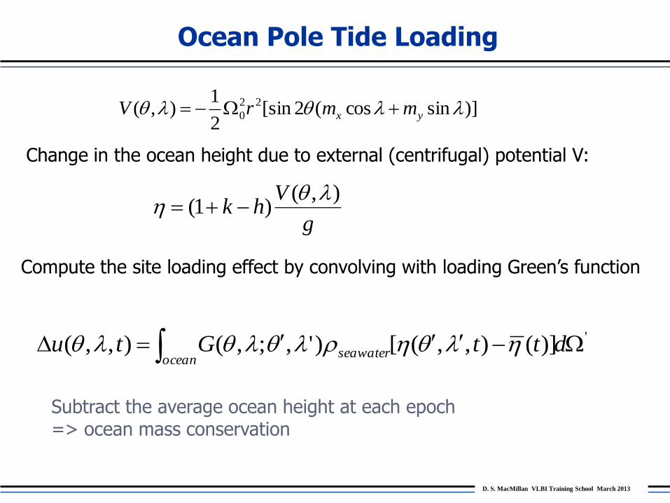
Ocean Pole Tide Loading
Change in the ocean height due to external (centrifugal) potential V:
g
Vhk
),()1(
Compute the site loading effect by convolving with loading Green’s function
')](),,([)',;,(),,( dttGtuocean
seawater
)]sincos(2[sin2
1),( 22
0 yx mmrV
Subtract the average ocean height at each epoch => ocean mass conservation
D. S. MacMillan VLBI Training School March 2013
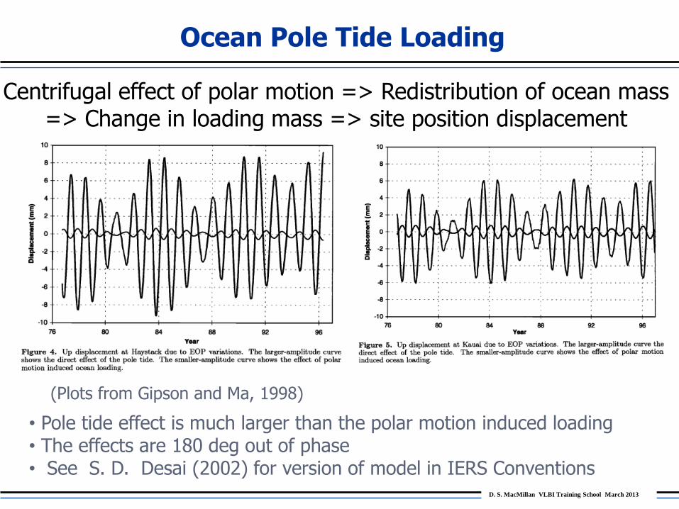
Ocean Pole Tide Loading
Centrifugal effect of polar motion => Redistribution of ocean mass => Change in loading mass => site position displacement
(Plots from Gipson and Ma, 1998)
• Pole tide effect is much larger than the polar motion induced loading • The effects are 180 deg out of phase • See S. D. Desai (2002) for version of model in IERS Conventions
D. S. MacMillan VLBI Training School March 2013
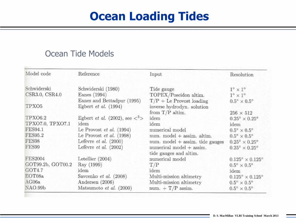
Ocean Loading Tides
Ocean Tide Models
D. S. MacMillan VLBI Training School March 2013
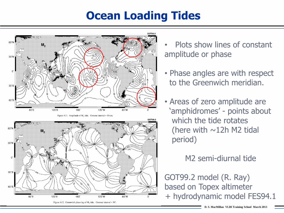
Ocean Loading Tides
• Plots show lines of constant amplitude or phase • Phase angles are with respect to the Greenwich meridian. • Areas of zero amplitude are ‘amphidromes’ - points about which the tide rotates (here with ~12h M2 tidal period)
M2 semi-diurnal tide
GOT99.2 model (R. Ray) based on Topex altimeter + hydrodynamic model FES94.1

D. S. MacMillan VLBI Training School March 2013
Ocean Loading Tides
O1 diurnal tide
GOT99.2 model

D. S. MacMillan VLBI Training School March 2013
Ocean Tidal Loading
• Tide elevation from global tide maps, where Z and δ are the amplitudes and phases of each specific partial tides k at
)],(cos[),(),,,( kkkk tZtk
• Loading at a site has to be computed by globally integrating the loading Green’s function over the tide elevation mass for each tidal constituent
Computation of ocean tidal loading
• Response of oceans to the Tide Generating Potential is much different than for solid earth • Response depends strongly on local/regional conditions
),(

D. S. MacMillan VLBI Training School March 2013
Ocean Tidal Loading
),,(,))(cos()(11
1
NEUktAtxj
kjjkjk
For each partial ocean tide, the tide crest occurs Φkj hours after the crest of the solid earth tide at the Greenwich meridian.
The astronomical argument of the tide
1) Loading UEN amp/phase are computed for 11 main tides (M2,S2,N2,K2,K1,O1,P1,Q1,Mf,Mm,Ssa) e.g., at Scherneck website 2) Better to also use HARDISP routine that computes loading based on 342 constituents found by interpolating tidal admittances based on the 11 main tides. (Error too large if keep only the 11 tide contribution) See IERS 2010 Conventions.
Site displacement due to loading is given by a sum over tides

D. S. MacMillan VLBI Training School March 2013
Ocean Loading Tides
Loading tables for other sites can be obtained at: http://froste.oso.chalmers.se/loading OR http://geodac.fc.up.pt/loading/index.html
D. S. MacMillan VLBI Training School March 2013
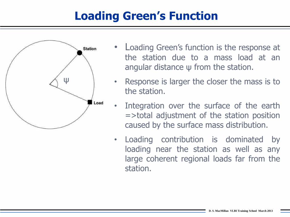
Loading Green’s Function
• Loading Green’s function is the response at
the station due to a mass load at an angular distance ψ from the station.
• Response is larger the closer the mass is to the station.
• Integration over the surface of the earth =>total adjustment of the station position caused by the surface mass distribution.
• Loading contribution is dominated by loading near the station as well as any large coherent regional loads far from the station.
ψ
D. S. MacMillan VLBI Training School March 2013
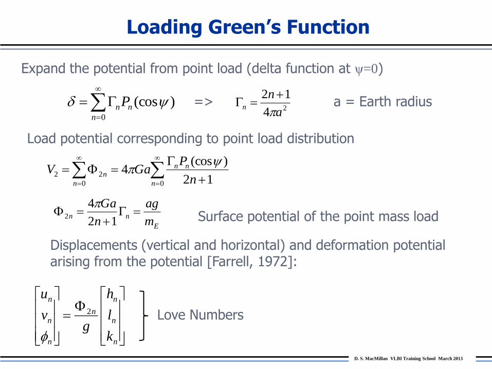
Loading Green’s Function
Expand the potential from point load (delta function at ψ=0)
0
)(cosn
nnP 24
12
a
nn
E
nnm
ag
n
Ga
12
42
Displacements (vertical and horizontal) and deformation potential arising from the potential [Farrell, 1972]:
n
n
n
n
n
n
n
k
l
h
gv
u2
Love Numbers
Surface potential of the point mass load
=>
0 0
2212
)(cos4
n n
nnn
n
PGaV
a = Earth radius
Load potential corresponding to point load distribution
D. S. MacMillan VLBI Training School March 2013
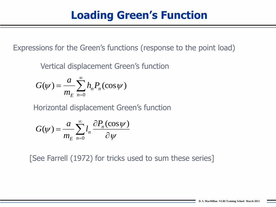
Loading Green’s Function
Vertical displacement Green’s function
0
)(cos)(n
nn
E
Phm
aG
Horizontal displacement Green’s function
0
)(cos)(
n
nn
E
Pl
m
aG
Expressions for the Green’s functions (response to the point load)
[See Farrell (1972) for tricks used to sum these series]

D. S. MacMillan VLBI Training School March 2013
Loading Green’s Function

D. S. MacMillan VLBI Training School March 2013
Loading Green’s Function
)( RG
)( HG
(Angular separation of site and load)

D. S. MacMillan VLBI Training School March 2013
Loading Green’s Function
'')'cos()(),','(),,( ddGtmtu Rv
'')'cos()(),','()cos(
)sin(
),,(
),,(
ddGtm
tu
tuH
N
E
is the angle between the vector pointing from the site to the mass point and the site local reference direction (north)
• We need to set up an appropriate grid for integration • The Green’s function is singular => the grid must be increasingly finely
divided the closer the mass points are to the site (as -> 0) to account for the rapid increase in the Green’s function.
D. S. MacMillan VLBI Training School March 2013
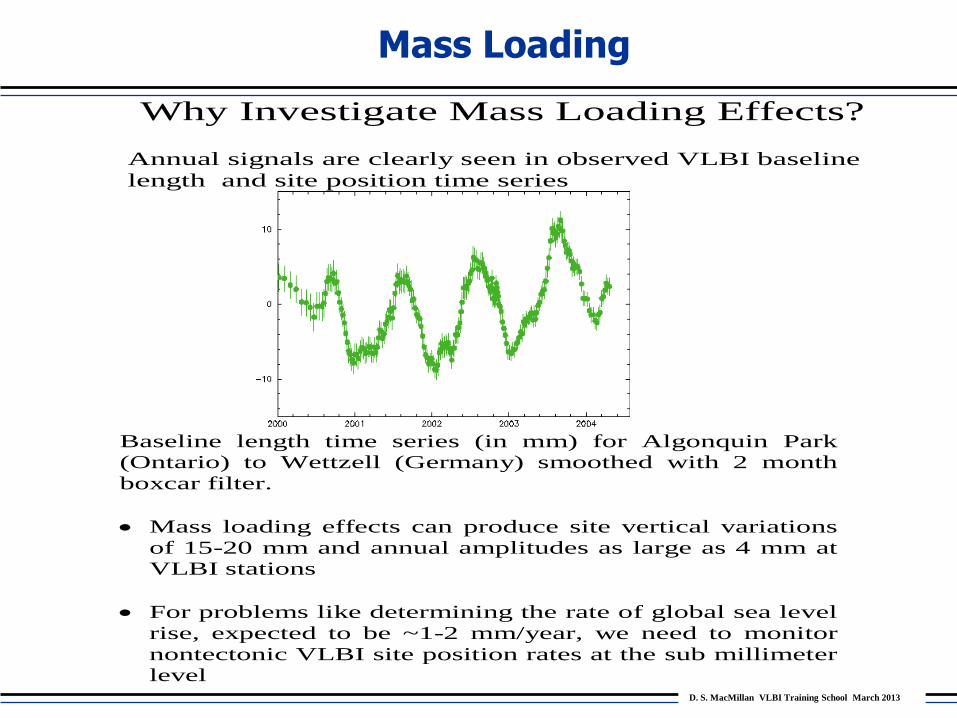
Mass Loading
Why Investigate Mass Loading Effects?
Annual signals are clearly seen in observed VLBI baseline
length and site position time series
Baseline length time series (in mm) for Algonquin Park
(Ontario) to Wettzell (Germany) smoothed with 2 month
boxcar filter.
Mass loading effects can produce site vertical variations
of 15-20 mm and annual amplitudes as large as 4 mm at
VLBI stations
For problems like determining the rate of global sea level
rise, expected to be ~1-2 mm/year, we need to monitor
nontectonic VLBI site position rates at the sub millimeter
level

D. S. MacMillan VLBI Training School March 2013
Effect of Pressure Loading at Westford
-10
-8
-6
-4
-2
0
2
4
6
8
10
12
2006 2006.5 2007 2007.5 2008 2008.5 2009
Ve
rtic
al
(mm
)
Pressure Loading Sensitivity ~ 0.2 – 0.6 mm/mbar
D. S. MacMillan VLBI Training School March 2013
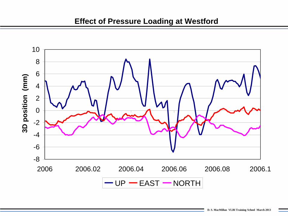
Effect of Pressure Loading at Westford
-8
-6
-4
-2
0
2
4
6
8
10
2006 2006.02 2006.04 2006.06 2006.08 2006.1
3D
po
sit
ion
(m
m)
UP EAST NORTH
D. S. MacMillan VLBI Training School March 2013
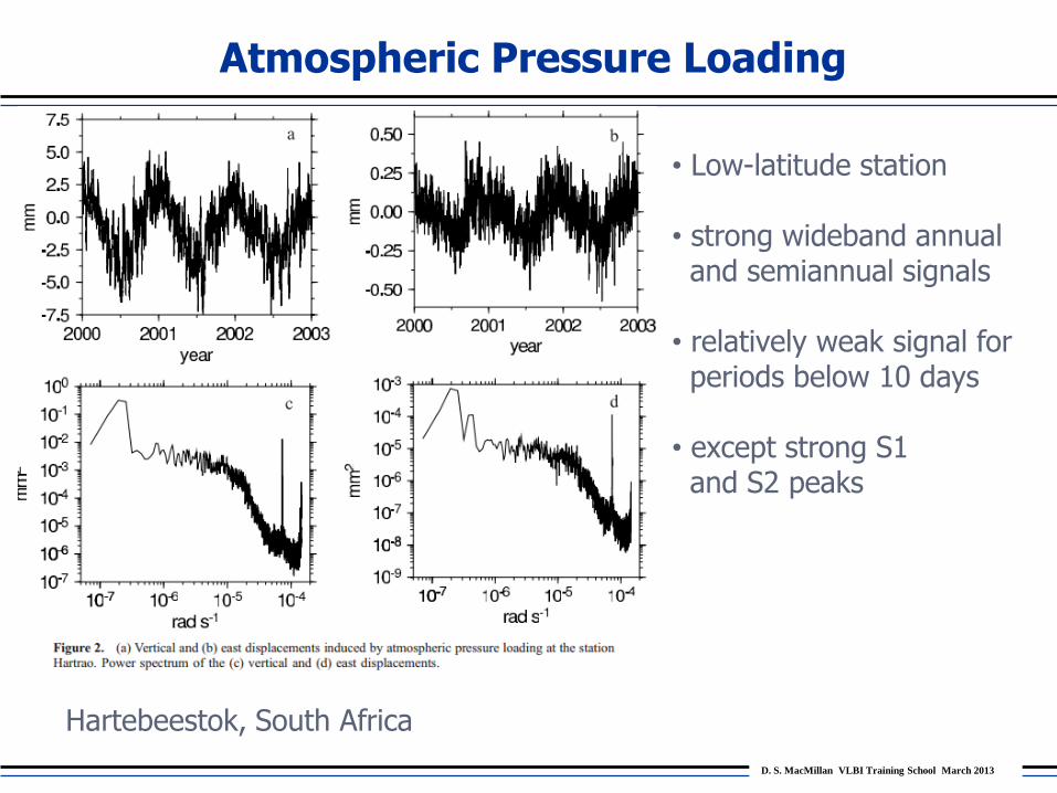
Atmospheric Pressure Loading
• Low-latitude station • strong wideband annual and semiannual signals • relatively weak signal for periods below 10 days • except strong S1 and S2 peaks
Hartebeestok, South Africa
D. S. MacMillan VLBI Training School March 2013
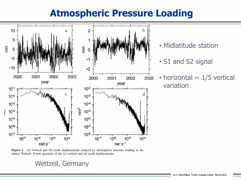
Atmospheric Pressure Loading
• Midlatitude station • S1 and S2 signal • horizontal ~ 1/5 vertical variation
Wettzell, Germany

D. S. MacMillan VLBI Training School March 2013
Atmospheric Pressure Loading
• Simple local loading model:
• Pressure loading admittance, α
estimated from VLBI data (mm/mbar) • Estimated admittances closer to convolution model admittances, where inverted barometer was assumed
)( refpressure PPUp

D. S. MacMillan VLBI Training School March 2013
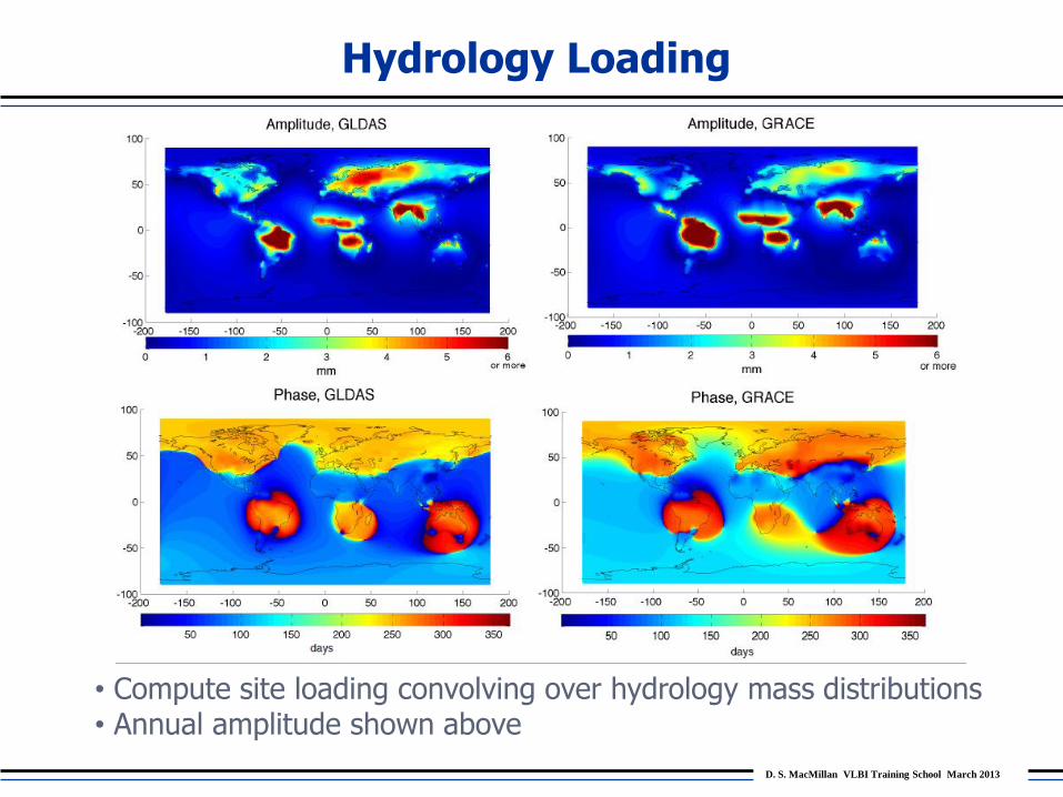
Hydrology Loading
• NASA GLDAS hydrology model (Rodell et al. 2004)
• Contributions from soil moisture, snow water, plant canopy
surface water storage
GRACE mass is in equivalent cm of water
D. S. MacMillan VLBI Training School March 2013
Hydrology Loading
• Compute site loading convolving over hydrology mass distributions • Annual amplitude shown above
D. S. MacMillan VLBI Training School March 2013
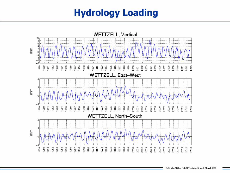
Hydrology Loading
D. S. MacMillan VLBI Training School March 2013
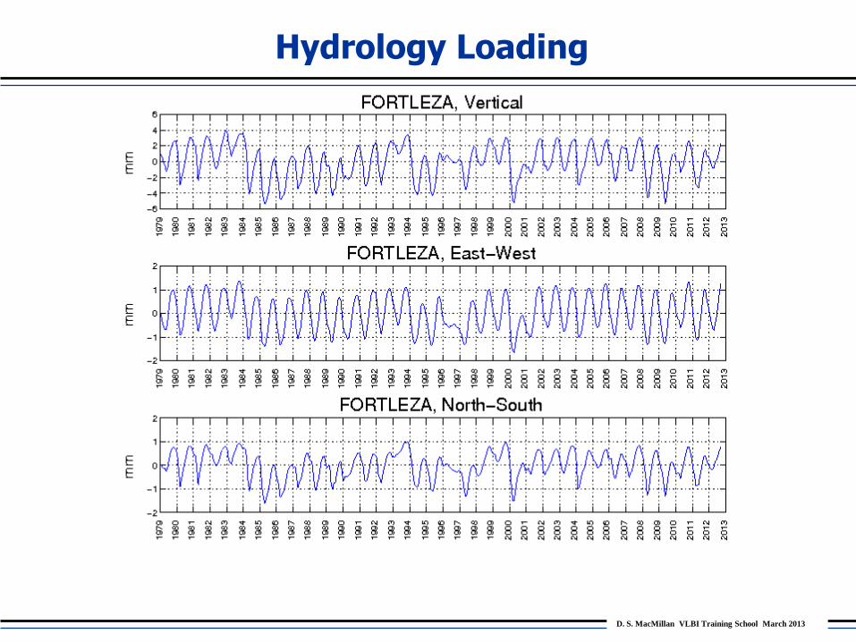
Hydrology Loading
D. S. MacMillan VLBI Training School March 2013
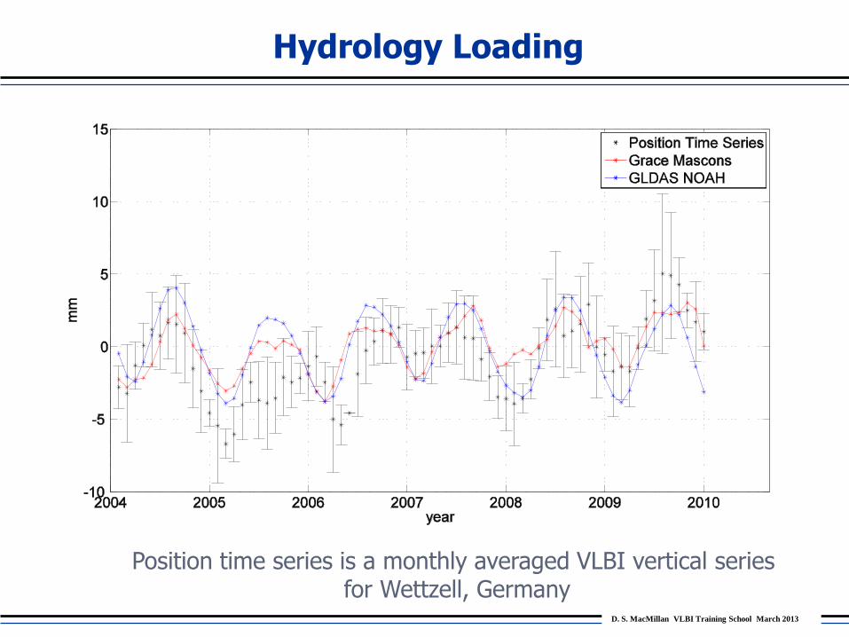
Hydrology Loading
Position time series is a monthly averaged VLBI vertical series for Wettzell, Germany

D. S. MacMillan VLBI Training School March 2013
Nontidal Ocean Loading
• JPL ECCO ocean model • Used 12-hour ocean bottom pressure since 1993 • Oceanic volume (not mass) conserving • Site displacement loading computed by usual Green’s function approach

D. S. MacMillan VLBI Training School March 2013
• Typical vertical loading series at VLBI sites: Coastal sites: Matera (Italy) rms 1.18 mm, Onsala (Sweden) rms 0.85 mm, Tsukuba(Japan) rms 0.89 mm Inland site: Wettzell (Germany) rms 0.31 mm • RMS variation is much smaller than VLBI residual vertical RMS
Nontidal Ocean Loading

D. S. MacMillan VLBI Training School March 2013
Nontidal Loading Series
Hydrology Loading • GLDAS NOAH model since 1979, updated when data is available • Monthly series for 170 VLBI stations • 1x1 degree gridded map with loading series for each lattice point • http://lacerta.gsfc.nasa.gov/hydlo/
Nontidal Ocean Loading • JPL ECCO model since 1993, updated when data is available • 12-hour resolution series for 170 VLBI stations • 1x1 degree gridded map will be generated in future • http://lacerta.gsfc.nasa.gov/oclo/
Atmospheric Pressure Loading • Maintain Petrov-Boy series • NCEP Reanalysis since 1979, updated when data is available • 6-hour series for 824 VLBI+GPS+SLR sites • 2.5x2.5 degree gridded map with loading series for each lattice point • http://lacerta.gsfc.nasa.gov/aplo_eph/

D. S. MacMillan VLBI Training School March 2013
Antenna Thermal Deformation
See A. Nothnagel (2009) for more on deformation model for all types of antenna mounts
Expansion coefficients γ ~ 1.0-1.2 x10⁻⁵/ºC

D. S. MacMillan VLBI Training School March 2013
-6
-5
-4
-3
-2
-1
0
1
2
3
4
1999.5 2000 2000.5 2001 2001.5 2002 2002.5
Th
erm
al
Exp
an
sio
n (
mm
)
GILCREEK
Fairbanks, Alaska antenna height ~ 15 m, annual temperature swing ~ 40 K,
expansion coefficient ~ 1.2x10-5 => peak-to-peak variation ~ 7 mm
Antenna Thermal Deformation
D. S. MacMillan VLBI Training School March 2013
Farrell, W.E., Deformation of the earth by surface loads, Rev. Geophys. Space Phys., 10, 761-797, 1972. Hartmann, T., and H.-G. Wenzel, The HW95 tidal potential catalogue, Geophys. Res. Lett., 22, no. 24, 3553-3556, 1995. Petit, G. and B. Luzum (eds.) , IERS Conventions (2010), IERS Tech. Note 36, International Earth Rotation and Reference Systems Service, 2010. Ray, R.D., A global ocean tide model from TOPEX/POSEIDON altimetry: GOT99.2, NASA/TM-1999-209478, NASA Goddard Space Flight Center.
References