georeferencing of scanned historical fsa aerial

Georeferencing of Scanned Historical FSA Aerial Photographs for Extraction of Wetlands Boundaries and Other Information for the Michigan NRCS Colin Brooks, Michelle Wienert, Luke Spaete, and Rick Dobson

May 2008

Michigan Tech Research Institute (MTRI) 3600 Green Court, Suite 100 • Ann Arbor, Michigan 48105

(734) 913-6840 (p) • (734)913-6880 (f) www.mtri.org

Georeferencing of Scanned Historical FSA Aerial Photographs for Extraction

of Wetlands Boundaries and Other Information for the Michigan NRCS

Colin Brooks, Michelle Wienert, Luke Spaete, Rick Dobson

May 2008

Georeferencing of Scanned Historical FSA Aerial Photographs MTRI • i

Table of Contents

Executive Summary.............................................................................................................. 1

Methodology.......................................................................................................................... 2

County Setup ................................................................................................................. 2 Georeferencing .............................................................................................................. 2

Results ................................................................................................................................... 6

Issues ................................................................................................................... 7

Conclusions .......................................................................................................................... 9

Acronym List ..................................................................................................................Acr-1

Appendix A: Detailed Methods for Georeferencing NRCS Aerial Photographs ....App-1

Georeferencing of Scanned Historical FSA Aerial Photographs MTRI • ii

List of Figures Figure 1: An example of a high-quality feature in common between the FSA

photograph and an NAIP image. ........................................................................ 2 Figure 2: An example of a just-completed aerial photo georeferenced in ArcGIS,

with an RMS error of 1.88-m................................................................................ 3 Figure 3: Points were easily found in common with adjancent photos due to

nine small circles being drawn on each photo; the top three from one image lined up with the bottom three in another. ............................................... 4

Figure 4: Example Image Index. ......................................................................................... 5 Figure 5: A map of the counties georeferenced as part of this project................................ 6 Figure A-1: Using command line to create excel spreadsheets for recording

RMS records. ................................................................................................App-1 Figure A-2: Georeferencing techniques. ........................................................................App-2 Figure A-3: Recommended 5 GCP locations...................................................................App-3 Figure A-4: Georeferencing Toolbar................................................................................App-3 Figure A-5: Red block shows aprx. area to zoom into when georeferencing

A1_xxxx. Red oval shows georeferencing toolbar. .......................................App-4 Figure A-6: Aligning ungeoreferenced images to georeferenced images

(in succession). .............................................................................................App-5 Figure A-7: Creating an Image Index. .............................................................................App-6 Figure A-8: Map of Michigan Counties and UTM 16N and 17N Zones. ..........................App-8

List of Tables Table 1: A list of the counties completed for the geoferencing project .................................. 7

Georeferencing of Scanned Historical FSA Aerial Photographs MTRI • 1

Executive Summary The MTRI geospatial team georeferenced 11,403 scanned historical aerial Farm Services Agency (FSA) photos using ESRI Desktop ArcGIS. These photos covered all of Michigan’s Lower Peninsula, plus two Upper Peninsula Counties, accounting for 84% of Michigan’s counties and 87% of the FSA scanned aerial photographs. The US Department of Agriculture (USDA) Natural Resources Conservation Service (NRCS) asked MTRI to georeference these photos because of valuable wetlands boundaries information that was recorded in pen only on these photos, which dated mostly from the late 1980s to early 1990s. With accurate georeferencing, this information could be directly digitized into a geospatial database for use by NRCS and other interested parties. The NRCS is now engaged in digitizing the wetlands data from the aerial photographs now that our georeferencing for 70 higher-priority counties is complete.

For this project, MTRI developed a standardized methodology to rapidly and accurately georeference thousands of aerial photographs. While making use of Desktop ArcGIS tools, we used our experience with imagery archives and vector data to create a method that could be applied to quickly processing large collections of imagery collections into a useful data set with earth coordinates (Universal Transverse Mercator, in this case). The methodology used recent aerial imagery, accurate road vector data, visual image interpretation, and features in common between scanned photos to create the fast and accurate georeferencing. This methodology could easily be applied to other imagery data sets for the NRCS and other interested agencies.

An important part of this project was the role that MTRI interns filled in completing the county georeferencing in a timely manner for NRCS. Between November, 2005 and May, 2008, the georeferencing process provided the opportunity for 19 interns to learn about GIS and remote sensing, including understanding imagery characteristics and processing spatial data. Three of them went on to become NRCS research scientists after starting as part of our georeferencing team.

With 13 counties remaining in Michigan, our hope is that the opportunity will exist to complete this data set for NRCS in the near future. With these image now available to NRCS in a geospatial format, they will provide a useful to integrate historical landscape information as well as provide an additional resource to understanding how Michigan’s lands are changing over time.


Methodology The complete methodology is included as Appendix A, “Georeferencing NRCS Aerial Photographs”, written by Assistant Research Scientist Luke Spaete. It describes each step of the process MTRI used to georeference the aerial photos. Our process had three main steps: 1) setting up Counties for georeferencing, 2) georeferencing, and 3) quality control and file packaging.

County Setup

The first step in the County setup process was to transfer the images from a 500-gigabyte USB drive to our main file server. After this, we created a list of all the images, which were in Lizardtech’s “MrSid” (or .sid) format, using file piping and Microsoft Excel. This provided a check list that would be used to keep track of completed photos and georeferencing accuracy. Finally, an ArcMap document (.mxd) was created with the correct County 2005 National Agricultural Imagery Program (NAIP) 1-m resolution orthorectified image. The UTM zone of the NAIP was checked against a map provided by Brent Stinson, Michigan NRCS GIS Analyst, of the official NRCS designations of UTM zones for each County. If there was a discrepancy, then we reprojected the NAIP image into the NRCS UTM zone using Lizardtech’s GeoExpress software. We also used ERMapper 7.0 and 7.1 to convert the county-wide NAIP files from MrSid format to ECW format, which loaded significantly faster in Desktop ArcGIS.

Georeferencing

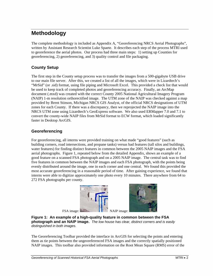
For georeferencing, all interns were provided training on what made “good features” (such as building corners, road intersections, and propane tanks) versus bad features (tall silos and buildings, water features) for finding distinct features in common between the 2005 NAIP images and the FSA aerial photographs. Figure 1, repeated below from the detailed Appendix, shows an example of a good feature on a scanned FSA photograph and on a 2005 NAIP image. The central task was to find five features in common between the NAIP images and each FSA photograph, with the points being evenly distributed around the image, one in each corner and one central. We found this provided the most accurate georeferencing in a reasonable period of time. After gaining experience, we found that interns were able to digitize approximately one photo every 10 minutes. There anywhere from 64 to 272 FSA photographs per county.

FSA image: NAIP image:

Figure 1: An example of a high-quality feature in common between the FSA photograph and an NAIP image. The low house has clear, distinct corners and is easily distinguished in both images.

The Georeferencing Toolbar provided the interface in ArcGIS for selecting the points and entering them as tie points between the ungeoreferenced FSA images and the correctly spatially positioned NAIP images. This toolbar also provided information on the Root Mean Square (RMS) error of the


five tie points used for georeferencing (see Figure 2, where an RMS of 1.88 is being displayed for a photo in Delta County). The RMS error was recorded for every photo so that MTRI could revised photos with a high RMS, and the NRCS could benefit from knowing the relative accuracy of each photo. Our georeferencing team aimed for an RMS error of below 5 meters, which was achieved for all but a handful (~2%) of photos. Photos in areas of greater elevation change tended to have higher RMS errors, but we still found it possible to make them line up accurately, sometimes using additional tie points to help.

Figure 2: An example of a just-completed aerial photo georeferenced in ArcGIS, with an RMS error of 1.88-m.

A key component of making the georeferencing process faster was taking advantage of a feature of the FSA photographs. Each FSA photo had nine circles drawn in nine corners (see Figure 3, repeated from the appendix), with the top three lining up with the bottom three of the previous image when they images started with the same letter (such as all the “N” images for a County). We used the top three and bottom three to make the images line up quickly, and then added our five high-accuracy points. This significantly speeded up the process (from about 20 to 10 minutes per photo) as it was no longer necessary to georeference each image to the NAIP image from scratch.


Figure 3: Points were easily found in common with adjancent photos due to nine small circles being drawn on each photo; the top three from one image lined up with the bottom three in another. The blue squares and red arrows show this alignment, which speeded up the georeferencing process.

A key part of our work was a well-documented and enforced Quality Assurance / Quality Control (QA/QC) process. First, any RMS errors above 6 meters were re-georeferenced to see if they could be made lower; later, our georeferencing team adopted a 5 meter standard as a goal. An MTRI researcher (first Luke Spaete, and later Michelle Wienert) checked images visually for positioning errors. Also, the researcher made sure that both geoferencing files were created (ending with .sdw and .aux.xml) for each photo. After this, Research Scientist Colin Brooks checked between 10 and 15 images per County to look for remaining positioning issues, using the high-accuracy Michigan Geographic Framework (MGF) roads as the comparison layer since it was independent of the NAIP imagery. If georeferenced images were found that did not line up well with the MGF roads, they were georeferenced, and neighboring images were checked to see if they also had positioning issues. This process of using two more senior staff members to check the interns’ work helped ensure a high-quality product for the NRCS.

After all QA/QC steps were complete, an “Image Index” was then created to show the extent and filename of each photo for a county. Brent Stinson from Michigan NRCS requested this so that the images would be easier to locate, especially by District NRCS staff who would also be using these images to locate important historical information such as the wetlands designations. We used a script, “Create Raster Index” (from http://arcscripts.esri.com/details.asp?dbid=14267) to create the image index. In the script version we applied, the final step after creating the index was to assign the correction projection to the resulting shapefile, either UTM, Zone 16, NAD83 or UTM, Zone 17, NAD83. Figure 4 shows an example of the image index for Emmet County, with the green lines showing image boundaries and the yellow callout boxes showing examples of the index captured the image names.


Figure 4: Example Image Index. Green lines depict image boundaries; yellow callout boxes shown how the image index includes identifying name information.


Results Our process meant that we provided 11,403 georeferenced photos to the NRCS over a 30-month period, or approximately 380 photos per month (about three typical counties). Our production rate was significantly higher during the summers of 2006 and 2007, when we had more intern staff than during the school year; also, summer staff was full-time. We found that balancing georeferencing with other GIS and remote sensing activities ensured higher productivity than assigning only georeferencing to our intern staff.

Our georeferencing was found by NRCS to be of sufficiently high accuracy that they were able to digitize wetlands boundaries directly from them, rather than the original intended method of picking out the boundaries from orthorectified images. This helped the NRCS capture the historical data more rapidly.

Figure 5 shows which counties have been completed as of the end of the NRCS project. The 11,403 photos completed by MTRI staff for this project mean that 1,706 remain, all in Upper Peninsula Counties. Table 1 lists the counties, and includes the number of photos per county.

Figure 5: A map of the counties georeferenced as part of this project. 70 of Michigan’s 83 counties (84%) were georeferenced by MTRI staff, which included 87% of the photos in the NRCS archive of FSA historical aerials.


Table 1: A list of the counties completed for the geoferencing project. The number of photos per county is also listed to show how totals varied.

County Photos County Photos Alcona 155 Lake 112 Allegen 233 Lapeer 193 Alpena 143 Leelenau 141 Antrim 152 Lenawee 213 Arenac 130 Livingston 163 Barry 180 Macomb 82 Bay 156 Manistee 144 Benzie 64 Mason 119 Berrien 137 Mecosta 168 Branch 170 Midland 129 Calhoun 224 Missaukee 138 Cass 180 Monroe 176 Charleviox 92 Montcalm 223 Cheboygan 131 Montmorency 96 Clare 130 Muskegon 133 Clinton 156 Newaygo 272 Crawford 76 Oakland 244 Delta 234 Oceana 155 Eaton 169 Ogemaw 144 Emmet 112 Osceola 166 Genesee 220 Oscoda 97 Gladwin 126 Otsego 115 Grand Traverse 145 Ottawa 196 Gratiot 168 Presque Isle 111 Hillsdale 170 Roscommon 76 Houghton 200 Saginaw 181 Huron 264 Sanilac 273 Ingham 156 Shiawassee 155 Ionia 182 St. Clair 186 Iosco 108 St. Joseph 180 Isabella 168 Tuscola 236 Jackson 255 Van Buren 195 Kalamazoo 174 Washtinaw 192 Kalkaska 171 Wayne 74 Kent 251 Wexford 143

Total: 11,403 Images

Issues

While georeferencing, we were able to discover and when needed, overcome, several technical issues. One was related to the introduction of ArcGIS 9.2 about half-way through the process. ArcGIS 9.2 introduced a new file format method for providing metadata details (XML), rather than the .aux text files that existed in ArcGIS 9.1 and before. As a separate file, named .sdw, actually provided the geoferencing information to GIS software, this file format change did not provide any compatibility problems.


A more significant issue was that a limited number of counties (such as Wayne County) that sometimes produced .sdwx files instead of .sdw. We found that .sdwx files worked for providing sufficient georeferencing information to ArcGIS 9.2, but not versions 9.1 and 8.3 which were in use at many NRCS offices. We found that it was necessary to georeference photos on a computer that had ArcGIS 9.1 on it to produce compatible .sdw files. We determined that .sdwx files were only produced for FSA photographs that had a MrSid “pyramiding” level of 8 or above; most images had lower pyramiding levels (which indicate how many different compressed resolutions of imagery are available in a single image). Some of these images also produced only a .aux.xml file, which while being sufficient for ArcGIS 9.2, did not work in versions 9.1 or earlier. Georeferencing within 9.1 also solved that problem.

We also discovered that the georeferencing toolbar did not always actually operate in the initial release of ArcGIS 9.2. Fortunately, Service Pack 2 (SP2) for ArcGIS 9.2 solved this problem; we had installed version 9.2 just before SP2 was released.


Conclusions Our detailed georeferencing methodology meant that the NRCS received approximately 380 photos of correctly positioned photos per month over the course of this project, for a total of 11,403 photos. The georeferenced imagery was valuable to NRCS to capture historical wetlands boundaries information from the FSA photographs, and has also been used by district NRCS staff in Michigan. NRCS staff found our georeferencing to be of sufficiently high quality that features of interest could be directly digitized from the photos without additional steps.

The georeferencing methodology developed for this project by MTRI would be applicable to meet future image registration needs of the NRCS or other agencies. By ensuring quality through a rigorous QA/QC process, we were able to create an image database useful to the state office of a Federal agency. We look forward to future opportunities to helping the NRCS gain maximum value from its imagery archive.

Georeferencing of Scanned Historical FSA Aerial Photographs MTRI • Acr-1

Acronym List

FSA Farm Services Agency

GCP Ground Control Point

GIS Geographic Information Systems

MGF Michigan Geographic Framework

MTRI Michigan Tech Research Institute

NAIP National Agricultural Imagery Program

NRCS Natural Resource Conservation Service

QA/QC Quality Assurance / Quality Control

RMS Root Mean Square

SP2 Service Pack 2

USDA United States Department of Agriculture

UTM Universal Transverse Mercator

Georeferencing of Scanned Historical FSA Aerial Photographs MTRI • App-1

Appendix A: Detailed Methods for Georeferencing NRCS Aerial Photographs The purpose of the NRCS Georeferencing project is to transfer NRCS’s scanned aerial photographs into a spatial domain quickly but at the same time with as little error in the georeferencing process as possible. To minimize time and limit error we have developed a process for georeferencing a whole county of scanned images as a group. Our process is comprised of three steps: 1) county setup 2) georeferencing 3) quality check and packaging.

County Setup

County setup is also a three step process: 1) transfer unprocessed images to working folder 2) setup Excel spreadsheet 3) setup .mxd for georeferencing.

1) Transferring images

The NRCS georeferencing project spans two drives. The N: drive stores the ungeoreferenced images and the J: drive is where images are stored when they are being georeferenced and packaged. When preparing a county for georefencing, the county’s images must be transferred from the N: drive to the J: drive. The ungeoreferenced images can be found in N:\NRCS_data\Legacy_Master_Photos. Copy the county folder and paste it to J:\project\USDA-NRCS\Georeferencing\Master_Photos.

2) Excel spreadsheet setup

While georeferencing information, RMS error, who georeferenced, etc., is recorded for each image that is georeferenced. We store this data in the county’s excel spreadsheet. The excel spreadsheets are stored in J:\project\USDA-NRCS\Georeferencing\Georef_basedata and the naming convention is list_(the county you are georeferencing).xls. To create a new spreadsheet, simply open list_template.xls and save as following the naming convention above. To input the ungeoreferenced images names into the excel spreadsheet you must run command prompt. See Figure A-1 below for commands.

Figure A-1: Using command line to create excel spreadsheets for recording RMS records.


Once the txt file is created navigate to that counties working folder on the J: drive and copy the contents of the text file into the excel spreadsheet. The Excel spreadsheet should now be ready to go (Delete names from the excel spreadsheet that have names in the beginning (ex. Allegan_F16_1.sid) as you will not be georefencing these images).

3) ArcMap document (.mxd) setup

When setting up your .mxd the most important thing to check is that the image you are georeferencing to and the .mxd you are georefencing in are in the right projection. Before you setup an .mxd make sure you look at the map projection information for Michigan counties .mxd (attached) and determine what UTM zone your county should be in. The next step is to make sure them National Agriculture Imagery Program (NAIP) imagery you are georeferencing to is in the right projection. Open Arc Catalog and navigate to the NAIP image for the county to be georeferenced, J:\gis_data\010_BaseMaps\010_202_Imagery\NAIP\ (nc_(yourcounty), right click on the NAIP .sid file and go to properties. Under the XY coordinate system tab make sure the image matches the proper UTM zone. If there is a discrepancy in the utm zones let Colin know and he will reproject it for you or let Colin know and reproject it yourself, either way let Colin know. If the image looks good open a new .mxd and add that image in first. This will guarantee that you are georeferencing in the proper projection. Now start adding your ungeoreferenced images from the J: drive. You are ready to georeference. (A suggestion, an .ecw created from NAIP .sid files loads much faster then a NAIP .sid file. If a .ecw file does not exist contact Colin Brooks and he will provide one).

Georeferencing

As stated in the intro, the purpose of the NRCS project is to transfer NRCS’s scanned aerial photographs into a spatial domain quickly but at the same time with as little error in the georeferencing process as possible. To minimize time and maximize precision we are using 5 Ground Control Points (GCP) for each image.

Georeferencing Techniques

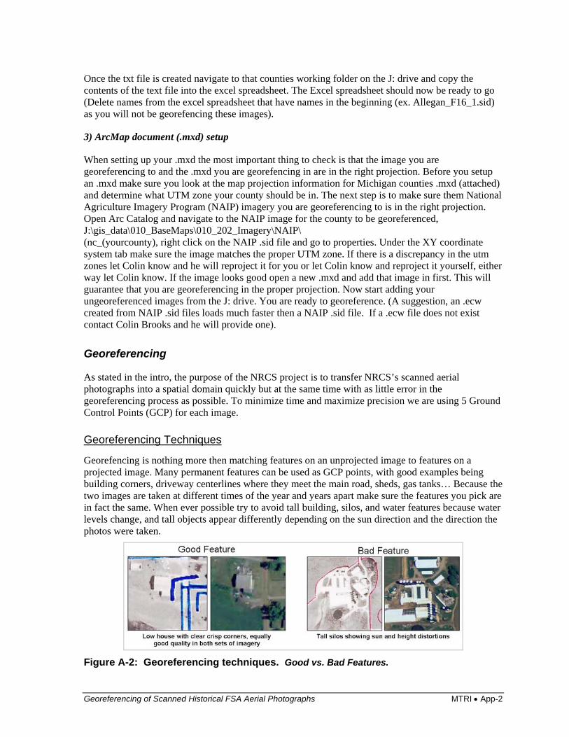
Georefencing is nothing more then matching features on an unprojected image to features on a projected image. Many permanent features can be used as GCP points, with good examples being building corners, driveway centerlines where they meet the main road, sheds, gas tanks… Because the two images are taken at different times of the year and years apart make sure the features you pick are in fact the same. When ever possible try to avoid tall building, silos, and water features because water levels change, and tall objects appear differently depending on the sun direction and the direction the photos were taken.

Figure A-2: Georeferencing techniques. Good vs. Bad Features.


For the purpose of this project we are only interested in adding 5 GCP points: one in the center and one in each corner (Figure A-3). It does not matter what order the GCP points are added.

Figure A-3: Recommended 5 GCP locations.

As each point is added the total Root Mean Square (RMS) error is calculated depending on how good of a job you have matched features from the ungeoreferenced image to the referenced image. At the end of the 5 points the RMS error should be around 3 but below 5.

Understanding the Georeferencing Toolbar

As shown in Figure A-4, the red circle is the layer you are georefencing. Make sure that the image you are georefencing is the same as the image name in that drop down menu. The blue arrow is the GCP tool. Make sure when you are adding a point that you add it first to the ungeorefenced image not the National Agriculture Imagery Program (NAIP) imagery. The red arrow is the RMS table. You can see the RMS error in this table and what points are contributing heavily to the RMS error. The blue circle is the update georeferencing option. This button is selected when you are done adding GCP points, you are happy with the RMS error, and you are ready to move on to the next image.

Figure A-4: Georeferencing Toolbar


Georeferencing Procedure

Beginning a County

Open the excel spreadsheet and the .mxd for the county you are working on. The NAIP imagery and the first of the ungeoreferenced images should already be loaded in the .mxd. The first image (A1_xxxxx) will always be in the upper left hand corner and is always the hardest one to georeference. Because of this a slightly different technique will be used to georeference this first one. Zoom to A1 by right clicking on the .sid A1_xxx and then left clicking on “zoom to layer”. Look for unique road features (interesting turns in roads, 6 way intersections), forest patterns, and/or discernable urban areas. Once you have a pretty good idea of the major features right click on the NAIP image and left click on “zoom to layer”. Using the magnifying glass in the tool toolbar zoom to the upper left hand corner of the NAIP image (Figure A-5). Try to find the same features in the NAIP image. Once you locate the same area GCP points can be added.

GCP points are a function of the georeferencing toolbar. On the main menu click on view>toolbars>and make sure georeferencing has tick by it. The tool should then be visible on the toolbar (figure 5). Using the GCP tool add the first point to the ungeoreferenced image then add the second point to the NAIP imagery (ALWAYS ADD THE FIRST POINT TO THE UNGEOREFERENCED IMAGERY!!!) Once the first point is added you can then continue to add the remaining 4 GCP points to the imagery in each of the 4 corners. When the image has 5 GCP points and the RMS is around 3 but below 5 go ahead and copy the RMS error to the excel sheet, along with the date you completed and who you are and then click update georeferencing (Keep an eye on the output directory when you update the georeferencing to make sure .sdw and .xml files are being written. If an .sdwx file is written or a lone .xml file are written contact your project manager). The image is now georeferenced and you are ready for your next image. Be sure to select the next image in the georeferencing drop down menu when you are done.

Figure A-5: Red block shows aprx. area to zoom into when georeferencing A1_xxxx. Red oval shows georeferencing toolbar.


Continuing a County

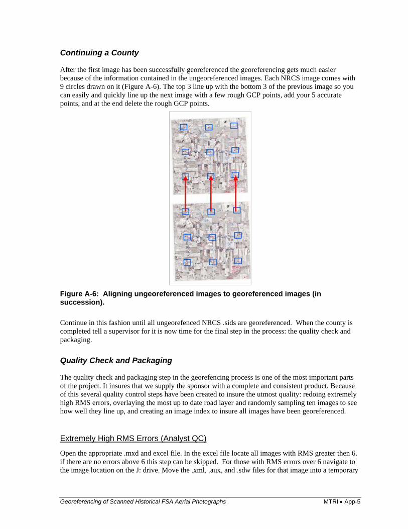
After the first image has been successfully georeferenced the georeferencing gets much easier because of the information contained in the ungeoreferenced images. Each NRCS image comes with 9 circles drawn on it (Figure A-6). The top 3 line up with the bottom 3 of the previous image so you can easily and quickly line up the next image with a few rough GCP points, add your 5 accurate points, and at the end delete the rough GCP points.

Figure A-6: Aligning ungeoreferenced images to georeferenced images (in succession).

Continue in this fashion until all ungeorefenced NRCS .sids are georeferenced. When the county is completed tell a supervisor for it is now time for the final step in the process: the quality check and packaging.

Quality Check and Packaging

The quality check and packaging step in the georefencing process is one of the most important parts of the project. It insures that we supply the sponsor with a complete and consistent product. Because of this several quality control steps have been created to insure the utmost quality: redoing extremely high RMS errors, overlaying the most up to date road layer and randomly sampling ten images to see how well they line up, and creating an image index to insure all images have been georeferenced.

Extremely High RMS Errors (Analyst QC)

Open the appropriate .mxd and excel file. In the excel file locate all images with RMS greater then 6. if there are no errors above 6 this step can be skipped. For those with RMS errors over 6 navigate to the image location on the J: drive. Move the .xml, .aux, and .sdw files for that image into a temporary


folder. Then load that image into the .mxd (it should show up ungeoreferenced) and try the georeferencing process over again. If you can not lower the RMS error then abandon the process and move the .xml, .aux, and .sdw files back to the proper directory. Do this for all images with RMS errors over 6.

Road Layer Check (Manager QC)

Open the appropriate .mxd. Load all georeferenced images back into the .mxd if they have been removed. Then add the most recent up to date road layer (currently J:\gis_data\018_Transportation\Michigan\MIGFv6b Roads.lyr). right click on Layers and select turn all layers off. Turn the road and NAIP imagery back on and 10 randomly selected NRCS images. In turn go through and check how the road layer and NRCS images line up at a scale of around 1:200. If you are happy with the result move on to creating an image index, if you are unhappy look up the RMS errors of the 10 NRCS images and try to diagnose the problem. After this, the images have passed intial QC.

Creating an Image Index (Analyst)

Open the appropriate .MXD. Go to tools>macros>visual basic editor. A visual basic window will pop up. Go to file>import file. Navigate to M:\software\windows\ESRI_Patches_and_Scripts\ Image_Index and select frmCreateRasterIndex.frm and press open. A Forms folder will show up on the right hand side of the visual basic window, open it and double click on frmCreateRasterIndex.frm. Make sure the window is selected and go to tools > references scroll down and check the box next to Microsoft Shell Controls and Automation and press ok. Once that is done the reference window goes away. Go to the top of the visual basic page and press the play button. The image index script should then run and should look like (Figure A-7).

Figure A-7: Creating an Image Index.


Click the add button and type in .sid after the asterisk and period, press ok. .sid should now be in the box below .ecw. highlight .ecw and press the del button. Click the search folder button and navigate to the appropriate folder where the georeferenced NRCS imagery is located. Change the name of the index shapefile to (nameofcounty_Image_Index). Press create index. It takes awhile but an image index shapefile without a projection defined gets added to the .mxd. You must define the projection as the same projection of the data frame as the script assumes the project of the index is GCS WGS84 when this is not the case. To do this click on the arctoolbox icon and navigate within the toolbox to Data Management tools> Projections and Transformations> define projection. Select the image index from the drop down menu and select the appropriate zone from the UTM NAD83 projections. Press ok. The image index should now be in the right location over the georeferenced NRCS images and the NAIP image. Right click on the image index and click zoom to layer. If the area moves way out and everything gets small that means there are images included in the index that have not been georeferenced. If you look closely you will see them on the lower part of the screen. Go ahead and use the magnifying glass to zoom in on them. Using the identify button click on them and all images that are ungeoreferenced will show up in the left column. If some do show up that should be georeferenced you must go back and georeference them and then recreate the image index. If they are images that do not have to be georeferenced (name_a14_34R.sid) use the editor toolbar to start editing select the polygons that shouldn’t belong and delete them. Make sure when you are done editing that you save edits and press stop editing. It is now time to package up the county for delivery to the sponsor.

Packaging

We supply the client with the .sdw and .xml files for each of the images we georeference, the county excel sheet, and the image index we created. We use Winzip to package our data for easy delivery. We do not include the .sid files!

Navigate to the georeferenced images (J:\project\USDA-NRCS\Georeferencing\Master_Photos\ (county)) create a WinZip file by right clicking in the folder new>winzip file. Name the file: (county)_georef_data.zip. Copy the .sdw and .xml files into the winzip folder. THIS IS ALSO A FINAL CHECK TO MAKE SURE THE RIGHT INFORMATION WAS WRITTEN WHEN GEOREFERNCING. LOOK FOR ANY INAPPRORAITE FILE TYPES IN THE DIRECTORY (ex. sdwx files, or only .xml files without the .sdw file) Next move the image index and all of its parts to the winzip folder and then add the appropriate excel document. Move the excel document to J:\project\USDA-NRCS\Georeferencing\Master_Photos\deliverable_ZIPS. Inform Colin of your completion

Clean-Up

The last step in the process is keeping the master_photo directory up to date. When a county is completed do the following: 1) delete the .sids out of the directory 2) move the directory to the completed counties folder, and 3) make a copy of the directory (now holding only .sdw and .xml files) and place it in the appropriate county folder on the n:/ drive.


Figure A-8: Map of Michigan Counties and UTM 16N and 17N Zones.

georeferencing of scanned historical fsa aerial

Documents