geostatistical modelling and simulation...
TRANSCRIPT

GEOSTATISTICAL MODELLING AND SIMULATION OF
UNCERTAINTY OF A KIMBERLITE PIPE
Nqangi Mjimba
A research project submitted to the Faculty of Engineering and the Built Environment,
University of the Witwatersrand, in partial fulfilment of the requirements for the
degree of Master of Science in Mining Engineering.
Johannesburg, 2013

2
DECLARATION
I declare that this research report is my own, unaided work. It is being submitted in partial
fulfilment of requirements for the Degree of Master of Science in Mining Engineering in
the University of the Witwatersrand, Johannesburg. It has not been submitted before for
any degree or examination in any other University. The information on which this
dissertation is based was obtained from Murowa Diamond Mine after request and
approval to use the mine for project purposes.
__________________________________________
(Signature of candidate)
________ day of __________________ ________

3
ABSTRACT
Understanding uncertainty associated with grades in resource models is an essential
requirement for mineral resource evaluation. One of the most important
considerations in diamond estimation is the use of an appropriate variable that
represents the true variability of grades in the kimberlite. The Spm3 variable used in
the Murowa pipes expresses true the variability of the grades in the kimberlite pipes.
Kriging in the Normal Scores (NS) approach and conditional geostatistical simulations
were used to investigate and quantify uncertainty of the grade in the KIMB4 unit of
the K1 pipe. The kriging in NS approach did not perform well in demarcating areas
that are truly high and those that are truly low in the estimates. Point realisations were
then generated using the sequential gaussian simulation algorithm. The resultant
conditional means and variances highlighted areas of high and low uncertainty in the
grade estimates. The point scale realisations were then averaged to the blocks size
used at Murowa (25m x 25m x 15m) to obtain the block conditional simulation model.
Zones of high and low uncertainties in the grade estimates of KIMB4 of the Murowa
K1 kimberlite were delineated and additional drilling was proposed to reduce the
uncertainty in the grade estimates. The uncertainty in grade was also investigated
down the pipe and this further identified the need for additional sampling at depth.

4
ACKNOWLEDGEMENTS
The author would like to thank Professor. R. Minnitt for his patience in supervising the
research project and for assistance in administrative matters at the University of the
Witwatersrand. Dr Chris Prins gave some valuable insight into the fundamentals of
diamond deposit evaluation. Special thanks go to Mr Lovemore Chimuka for all his
input and for supplying the data used in the study. Murowa Diamonds, the operating
company of Murowa Diamonds Mine, is thanked for granting me the opportunity to
conduct this study and the permission to publish this project report. I am grateful to
Dr. Ina Dohm who first fanned my interest in geostatistics. Lastly, a special thanks to
Dr Alexandre Boucher and his prompt assistance in matters relating to the availability
and use of the SGeMS software.

5
For my Husband
Ignatious Ncube

6
CONTENTS
DECLARATION ............................................................................................................ 2
ABSTRACT .................................................................................................................... 3
CONTENTS .................................................................................................................... 6
LIST OF FIGURES ........................................................................................................ 9
LIST OF TABLES ........................................................................................................ 12
LIST OF SYMBOLS .................................................................................................... 13
NOMENCLATURE ...................................................................................................... 14
1 INTRODUCTION ............................................................................................... 16
1.1 General Geology ............................................................................................ 16
1.2 Kimberlite Geology ....................................................................................... 19
2 FORMULATION OF THE PROBLEM .............................................................. 23
2.1 Justification for the current study .................................................................. 26
2.2 Parameters used in diamond grade estimation .............................................. 30
2.2.1 The appropriate variable for estimation ................................................. 30
2.2.2 Modifications necessary to combine different data sources .................. 32
2.2.3 The incorporation of calliper data for sample volume and density for
sample mass .......................................................................................................... 33
2.2.4 Inclusion or exclusion of incidental diamonds....................................... 33
3 EXPLORATORY DATA ANALYSIS ............................................................... 34
3.1 Data Validation .............................................................................................. 34
3.2 Data declustering ........................................................................................... 37
3.3 Variography of the domains of the K1 pipe .................................................. 38
4 GEOSTATISTICAL ANALYSIS OF THE SPM3 VARIABLE OF THE KIMB4
DOMAIN ...................................................................................................................... 42

7
4.1 Ordinary Kriging ........................................................................................... 42
4.2 Normal Scores variography of the KIMB4 domain ...................................... 46
4.3 Indicator Kriging of Spm3
variable ................................................................ 52
5 CONDITIONAL SIMULATION OF THE SPM3 VARIABLE OF THE KIMB4
DOMAIN ...................................................................................................................... 57
5.1 The Theory of Sequential Gaussian Simulation ............................................ 57
5.1.1 Validation of the simulations ................................................................. 60
5.2 The application of sequential gaussian simulation to the Spm3 variable ...... 60
5.2.1 Validation of the Spm3 variable simulation ........................................... 62
6 ASSESSING UNCERTAINTY IN THE KIMB4 DOMAIN .............................. 67
6.1 Measures of uncertainty ................................................................................ 68
6.2 Point kriging model ....................................................................................... 69
6.3 Quantile and Probability Maps ...................................................................... 72
6.4 Point Simulation Model ................................................................................. 74
6.5 Presentation of the block model .................................................................... 78
7 DISCUSSION ...................................................................................................... 86
8 CONCLUSIONS AND RECOMMENDATIONS .............................................. 90
8.1 Recommendations for Future Work .............................................................. 91
9 REFERENCES ..................................................................................................... 92
APPENDIX I- EXTRACT FROM THE JORC CODE: REPORTING OF DIAMOND
EXPLORATION RESULTS, MINERAL RESOURCES AND ORE RESERVES .... 96
APPENDIX II– EXPERIMENTAL HORIZONTAL VARIOGRAMS ....................... 99
APPENDIX III – INDICATOR VARIOGRAM MODELS FROM SPM3 > 5 TO SPM
3
>26 THRESHOLDS ................................................................................................... 102
APPENDIX IV-PROGRESSIVE STATISTICS DATA ............................................ 113

8
APPENDIX V-SUMMARY OF REALISATION STATISTICS .............................. 116
APPPENDIX VI- SELECTED INDIVIDUAL REALISATIONS ............................. 118
APPENDIX V11 –15m BENCH INTERVAL AND BLOCK KRIGING MAPS
OUTPUT COMPARED TO SIMULATED MAPS OUTPUT PER BENCH
INTERVAL ................................................................................................................. 120

9
LIST OF FIGURES
Figure 1: Schematic map showing the location of Murowa kimberlites and the regional
geology. ......................................................................................................................... 17
Figure 2: Location of the Murowa kimberlite pipes in relation to the main structural
features; to the west a doleritic dyke and to the east a shear zone. Notation shows the
K1-K5 pipes. ................................................................................................................. 18
Figure 3: K1 geology model showing the internal geology domains. The KIMB4
domain outline is highlighted in red. ............................................................................ 21
Figure 4: Inclined view of the K1 geology model ........................................................ 22
Figure 5: High grade vent surrounded by relatively low grade samples (left) and
sample grades within K1 showing smoothing of grades with no recognition of feeder
vent (right). Images from Platell (2011) ...................................................................... 26
Figure 6: Plan view of the K1 pipe, showing the location of LD drill holes in K1and
the MPZ domain (in pink) enveloping the other domains, and location of data points of
the KIMB2/4 domain in relation to the entire K1 pipe. Image from Platell (2011) ..... 35
Figure 7: Histograms for the KIMB1 domain (left); KIMB2/4 domains (middle) and
MPZ domain (right) ...................................................................................................... 36
Figure 8: Spherical model variogram for the Spm3 variable for KIMB4 in the vertical
direction......................................................................................................................... 39
Figure 9: Radar chart of Horizontal variogram ranges of the KIMB4 domain ............. 40
Figure 10: KIMB4 omni- directional spherical variogram model for the Spm3 variable
....................................................................................................................................... 41
Figure 11: Discretisation test used to determine the optimal block discretisation of
5x5x1 for the KIMB4 domain. ...................................................................................... 44
Figure 12: Cross validation of the Spm3 estimates from the KIMB4 domain .............. 45
Figure 13: The normal score transformation for data zi. At the bottom is the
anamorphosis function. Sourced from Ortiz and Deutsch (2003)................................ 47
Figure 14: Calculation of the mean by numerical integration. Sourced from Oritz and
Deutsch (2003) .............................................................................................................. 48

10
Figure 15: Normal scores transformation process and resultant parameters of the
KIMB4 Spm3 variable ................................................................................................... 49
Figure 16: Model variogram parameters for Spm3 data from the domain, modelled in
Gaussian space. ............................................................................................................. 50
Figure 17: Comparison of untransformed OK (left) and gaussian (NS) back-
transformed kriging map outputs (right) ....................................................................... 51
Figure 18: KIMB4 domain OK results (right) and SK back-transformed kriging results
(left) viewed from the SW............................................................................................. 52
Figure 19: Relationship between various cut-offs of Spm3 and the proportion above
cut-off (top) and the model indicator variogram at a cut-off of 12 Spm3. .................... 55
Figure 20: Kriged map of Spm3 >12 viewed from the top, as well as the block model
of the KIMB4 domain. .................................................................................................. 55
Figure 21: Cumulative frequency distribution of 10 randomly selected realisations in
NS (in blue) compared to the cumulative frequency of the input data (in red) ............ 63
Figure 22: The univariate statistical parameters of randomly selected histograms
generated from the Sequential Gaussian simulation of Spm3 compared to those of the
sample data (bottom left). ............................................................................................. 64
Figure 23: Frequency distribution of 10 randomly selected back-transformed
realisations (in blue) compared to the raw Spm3 data (in red) ..................................... 65
Figure 24: Experimental variograms of randomly selected realisations (crosses)
compared to the model of the input data (solid line) .................................................... 66
Figure 25: Map outputs of back-transformed NS kriging (left) compared to kriging in
NS with mean of zero (middle) and OK (right) showing the high grade area to the
South West of the domain and low grades estimates elsewhere. .................................. 70
Figure 26: Back-transformed NS Variance (Left) compared to the Kriging variances in
NS with mean of zero (middle) and OK( right) ............................................................ 71
Figure 27: NS Back-transformed mean map (right) compared to back-transformed
variances (Left) ............................................................................................................. 72
Figure 28: 0.05 (extreme left), 0.5 (middle left), 0.9 (middle right) probability maps
and NS back-transformed map (extreme right) ............................................................. 73

11
Figure 29: Map of conditional means (left) and conditional variances (right) ............. 75
Figure 30: Map outputs of probability maps at 0.1 quantile (extreme left), 0.5 quantile
(middle left), 0.9 quantile (middle right) compared to the conditional mean map
(extreme right) ............................................................................................................... 76
Figure 31: P10 and P90 maps flagging areas that are surely high (right) and areas that
are surely low in Spm3 estimates (left). ........................................................................ 77
Figure 32: Probability of Spm3 values above 0.2ct/t cut-off. ........................................ 78
Figure 33: Comparison of univariate statistical parameters of the Spm3 sample data
(top left) against those of the ordinary kriged estimates (top right) and mean of the
simulations (bottom left). The output from the kriging and simulation is also compared
using a quantile-quantile plot (bottom right) where ordinary kriged estimates are
plotted on the X-axis and the Conditional mean of the simulations on the Y-axis. ...... 79
Figure 34: Output from the different techniques generated by Kriging (left), SGS
(middle) and indicator kriging results (Prob Z*>12) right ........................................... 80
Figure 35: Map of Conditional means (left) and conditional variances (right) ............ 81
Figure 36: P10 (left) and P90 (middle) maps flagging blocks that are surely high and
blocks that are surely low in Spm3 estimates blocks where there is high uncertainty -
broken line (left) and conditional mean map (right). .................................................... 82
Figure 37: Block coefficient of variation and resource classification........................... 83
Figure 38: Proposed LD holes (pink) and P10 and P90 maps flagging blocks that are
surely high and blocks that are surely low in Spm3 estimates and blocks where there is
high uncertainty -broken line (middle and right). The magenta line outlines the KIMB
domains, the yellow line- weathering and the blue the MPZ. ....................................... 85
Figure 39: Post plots of Spm3 values on the geological model and in relation to the
areas of high and low uncertainty and resource classification based on COV. ............ 86
Figure 40: Comparison of the output of nineteen individual conditional simulations.
The ±15% envelope about the mean is shown as a reference. ...................................... 88
Figure 41: Spm3 Conditional simulated mean per bench along with the 95%
confidence limits. .......................................................................................................... 89

12
LIST OF TABLES
Table 1: Tabulation of findings that could have resulted in the deficit of 2009: Source
from Platell (2011) ........................................................................................................ 23
Table 2: Change in overall tonnes and carats between the 2010 and 2000 model (grey
fill). Source from Platell (2011) .................................................................................... 27
Table 3: Drillhole samples used for each domain ......................................................... 36
Table 4: The omni-directional semi variograms models from KIMB2/4 and MPZ
domains ......................................................................................................................... 41
Table 5: Table showing a comparison of the estimates and actual values of the KIMB4
....................................................................................................................................... 44
Table 6: Base statistics for CCOV and classification category..................................... 83

13
LIST OF SYMBOLS
Billion Years Ga
Gamma ɣ
Grams per Tonne g/t
Greater than >
Hectares ha
Kilometre km
Lamda λ
Less than <
Less than or equal to ≤
Metre m
Nugget Effect C0
Variogram Sill C1
Percent %
Tonnes t

14
NOMENCLATURE
Carats per tonnne ct/t
Carats per hundred tonnes cpht
Coefficient of variation COV
Cumulative distribution function cdf
Conditional Cumulative distribution function ccdf
East E
Direct block simulation DBSIM
Geostatistical Software Library GSLIB
Hypabyssal kimberlite HK
Injected granite IG
Inverse power distance IPD
Inter quartile range IQR
Joint Ore Reserves Committee Code JORC
Life of mine LOM
Large diameter reverse circulation LDRC
Murowa Expansion MXP
Marginal Pipe Zone MPZ
Mean Stone Size MSS
Mantle Xenolith MX
North N
North North West NNW
Normal Scores NS
Selective Mining Unit SMU
Sequential Gaussian Simulation SGS
Stanford Geostatistical Modelling Software SGeMS
Stones Per cubic metre Spm3
South South East SSE
South West SW

15
West W
Dollars per carat $/ct
16
1 INTRODUCTION
The Murowa kimberlite cluster is located in the South Eastern part of Zimbabwe,
about 200km from the border of South Africa, 60 km South West of Masvingo and
some 35 km South East of the town of Zvishavane. The Murowa kimberlite cluster
was discovered and evaluated between 1997 and 2000 as part of the regional
exploration program undertaken by Rio Tinto between 1994 and 2000 in Zimbabwe.
The K1 (2.6ha) and K2 (0.8ha) pipes have been mined since late 2004 by conventional
open-cast methods. Murowa Diamonds is the company that is responsible for mining
the kimberlites. Murowa Diamonds is an unincorporated joint venture between Rio
Tinto Zimbabwe (56% owned by Rio Tinto plc) and Tinto Holdings Zimbabwe (100%
owned by Rio Tinto plc.). The beneficial ownership is, therefore, 78% Rio Tinto plc
with the balance being held principally by investors through the Zimbabwe Stock
Exchange.
1.1 General Geology
The kimberlites are of Cambrian age, situated on the Archean Zimbabwe Craton. The
area lies at an elevation of 760m and is bounded immediately to the east by the Runde
River. The nearest previously recorded kimberlites are Chingwizi, Sese and others in
the Limpopo Mobile Belt.
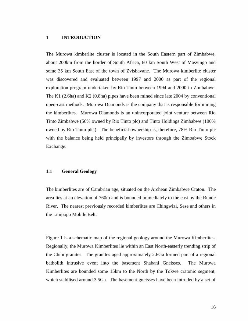
Figure 1 is a schematic map of the regional geology around the Murowa Kimberlites.
Regionally, the Murowa Kimberlites lie within an East North-easterly trending strip of
the Chibi granites. The granites aged approximately 2.6Ga formed part of a regional
batholith intrusive event into the basement Shabani Gneisses. The Murowa
Kimberlites are bounded some 15km to the North by the Tokwe cratonic segment,
which stabilised around 3.5Ga. The basement gneisses have been intruded by a set of
17
East South-easterly and East North-easterly trending dolerites, themselves cut by the
Chibi Granites. To the South, also about 15km, lies the East North-easterly trending
Mberengwa Greenstone belt of the Bulawayan System, which hosts a banded iron
formation, exploited at Buchwa for iron up until the late 1980s. The greenstone
formations were probably established by 2.8Ga and in the Buchwa area they are
contained as remnants within the Mweza Schist Belt.
Figure 1: Schematic map showing the location of Murowa kimberlites and the
regional geology.

18
A series of inselberg domes up to 250m high around Murowa, are said to attest to
stripping of the weathering profile by more recent erosion. Buhwa Mountain, 12km
south of Murowa and formed of banded ironstone, lies more than 600m above the
surrounding Pliocene–Quaternary plain and forms a remnant of the older Pre- Karoo
erosion surface (Mtetwa et al., 2002).
The Murowa Diamond deposit consists of a cluster of five kimberlite pipes and dykes.
The pipes, labelled K1 to K5, lie between two structural features with a North-South
trend (Figure 2). To the West is a doleritic dyke and to the east is a major shear zone.
Figure 2: Location of the Murowa kimberlite pipes in relation to the main structural
features; to the west a doleritic dyke and to the east a shear zone. Notation shows the
K1-K5 pipes.
K5
K1
K3
K2
K4

19
The K1 pipe is considered to be part of a complex blow along a North-South system of
kimberlite dykes of which the smaller K3, K4 and K5 bodies are a part of the local
controls on K1 are of North-South orientation. However K2’s emplacement was more
directly controlled by a reactivation along the shear zone.
The shape of the pipe of the K2 pipe, the eastern side of which is in direct contact with
the shear, and the western wall which dips away to the west, is an inverted wedge.
This shape is unusual for a kimberlite pipe and it is said almost certainly to result from
a structural preparation of the ground. Detailed observation of some dyke contacts
with the granite on the western side of K2 indicate that there was indeed some
reactivation along the quartz shear occurring at the time of emplacement.
Only K1, K2 and K3 are considered economic based on the OoM estimates. K1 and
K2 are currently being mined while K3, the smallest of the economic pipes with
lowest value ore will be mined after the two larger pipes have been completed. K1 and
K3 have similar grade profiles while K2 is somewhat different being significantly
higher in grade. Of the three pipes, K2 pipe shows a clear boundary between ore and
waste, whereas the ore in K1 and K3 has a halo of lower grade material referred to as
the MPZ. This material will be stockpiled for later treatment. Waste rock material is
predominantly granite.
1.2 Kimberlite Geology
The pipes themselves are exposed in the root zone at the current erosion level. The
small complex multi-lobed bodies together with sills and dykes are characteristic of
the basal part of kimberlite pipe development (Smith et al., 2004). The geology of the
Murowa kimberlite pipes is complex comprising of inter-mixing of kimberlite
lithologies and different phases of emplacement. The country rock is veined,
brecciated and/or metasomatised and fenitised with kimberlitic fluid phases at the

20
kimberlite pipe contact (Moss, 2010). The K1 pipe (the main focus of this study) is
modelled as a complex, steep sided multi-lobed kimberlite pipe. The contact zones
around K1 vary in thickness, overall rock textures and the relative proportion of
kimberlitic components. There are five kimberlite type domains in the K1 pipes
namely KIMB1, KIMB2, KIMB3, KIMB4 and KIMB5 as well as additional MPZ and
KDYKE-MX.
KIMB1 and KIMB5 consist of coherent kimberlite mainly a hypabyssal kimberlite.
KIMB2 and KIMB4 consist mainly of volcaniclastic kimberlite and KDYKE-MX is a
mantle xenolith-rich dyke. The MPZ is a granite-rich and kimberlite-poor or
kimberlite absent domain that is spatially distinct from the main pipe-filling domains
and it forms an envelope around the other domains. Figure 3 shows the geological
domains of the K1 pipe and Figure 4, the inclined view of the K1 geology model.

21
Figure 3: K1 geology model showing the internal geology domains. The KIMB4
domain outline is highlighted in red.

22
Figure 4: Inclined view of the K1 geology model
Of the K1 domains, KIMB4 is volumetrically dominant followed by KIMB1 and
KIMB2. KIMB5 represents a comparatively minor volume within the modelled depth
while KDYKE-MX is modelled as a surface, with no estimated volume. KIMB3 was
not modelled as a separate domain due to the lack of spatial continuity, spatial overlap
with other rock types, and the sub-mining scale (<5m) of most occurrences.

23
2 FORMULATION OF THE PROBLEM
During 2009, there was a shortfall in carats from the K1 pipe and Rio Tinto
Technology and Innovation (T&I) in Perth, Australia was engaged to perform a
desktop review of the existing K1 Murowa resource model that was constructed as
part of the Murowa feasibility study of 2000. The aim of this review was to identify
any potential issues with the existing model that may have caused an over-estimation
of resource grade. The review identified several issues that may have led to an over-
estimation of resource grade in this initial model. The findings are listed in Table 1.
Table 1: Tabulation of findings that could have resulted in the deficit of 2009: Source
from Platell (2011)
Issue
identified
Description of the issue
Conflicting
lithology
codes
There was little correlation between the domains as modelled
in the 2000 model and the lithology codes contained within
the database used.
A large number of codes used within the internal pipe did not
exhibit any clear internal domaining.
There were numerous instances where adjacent or crossing
holes were logged with conflicting codes, suggesting that
there was an issue with the standard of core logging in the
evaluation of 2000.
This was observed both in the vent as well as elsewhere in
the pipe.

24
The enriched
vent
The majority of the high grade samples occurred at the
southern end of K1 within a narrow feeder pipe, or “vent”,
with the remaining parts of the modelled pipe essentially very
low grade.
Shielding of
High Grade
Samples
In the 2000 model, samples greater than 140 spm3 were
shielded (capped) so that their influence was restricted to one
parent block (25m2). However, study of the sample grade
histograms indicated that the MPZ domain and the KIMB4
domain contained outliers in the grade distribution.
The outliers could have been left out in the production of the
variograms but included in the kriging and not restricted
Weathering
During the 2000 study that a weathering (or oxidation)
horizon may have a significant impact on the grade. The
weathered kimberlite may have been enriched due to
winnowing of non-diamond material.
The weathering surface that was used for the 2000 estimate
was inspected and found to be quite irregular, with many
peaks and troughs which did not appear to be supported by
the weathering code as logged in the drill hole database.
A new weathering surface was created from the existing
weathering data using the surface gridding technique in
Vulcan. As in the 2000 estimate the weathered surface was
not modelled as a separate domain due to the lack of spatial
continuity. This issue will not be considered in this study as
only the fresh un-mined material will be used in the estimate
Eastern Dykes
Within the MPZ domain, only three samples showed
significant grade. These samples were all located on the

25
eastern margin of the pipe and appeared to be aligned on a
north-south trend. T&I postulated that these samples
represented intersections of relatively narrow grade-bearing
dykes. This interpretation was supported by delineation hole
logging which indicated narrow intersections of kimberlite in
this area.
Density Media
Separation
Plant Issues
Issues were also identified in the process plant, such as
Density Media Separation efficiency and weightometer
accuracy but these issues were considered outside the scope
of the both the investigation by T&I as well as in the study
that will be undertaken.
The failure to recognise the feeder/enriched vent had the most significant influence on
the over estimation of the resource grade. This factor influenced the smoothing of
grades in the southern end of the K1 kimberlite pipe as shown on Figure 5. The
enriched vent was not recognised in the 2000 evaluation. The result was that high and
low grade samples within the major domain were smoothed at the southern end of the
pipe. The smoothing approach could have resulted in an over-estimation of grade as
blocks outside of the vent would be unduly influenced by high grade samples within
the vent.
Conversely the low grade samples outside the vent would cause blocks within the vent
to be under-estimated, if the high grade vent was of a small volume relative to the
surrounding low grade area, this would lead to an overall over-estimation in grade
(Platell, 2011).

26
Figure 5: High grade vent surrounded by relatively low grade samples (left) and
sample grades within K1 showing smoothing of grades with no recognition of feeder
vent (right). Images from Platell (2011)
Mineral Services Canada Inc. (MSC) was then engaged in March 2010 to re-evaluate
the geological core logging and to re-model the internal geology of the K1 pipe. This
resulted in a revised geological model already discussed above in Section 1. T&I then
created a revised resource estimate based on this new interpretation. This new model
was expected to give a more realistic prediction of grade and consequently to give an
improved reconciliation once the new estimate is used during mine planning.
2.1 Justification for the current study
The detailed work by MSC indicated that the KIMB1 (vent) was much narrower than
had been modelled by T&I. The overall tonnage estimated decreased by over 5% in
K1, due to the changes in the interpretation kimberlite pipe. This was coupled with a
decrease of over 40% in carats within K1 (Table 2).

27
Table 2: Change in overall tonnes and carats between the 2010 and 2000 model (grey
fill). Source from Platell (2011)
Pipe Unit
Tonnes
(Million)
Carats
(Million) Unit
Tonnes
(Million)
Carats
(Million)
K1 KIMB1 0.64 1.08 HK 19.51 9.98
KIMB2 0.10 0.06
KIMB4 8.16 3.10
MPZ 19.01 2.04 IG 14.79 2.03
Total 27.91 6.28 Total 34.30 12.01
Based on the new resource model, T&I classified the KIMB1 and KIMB4 units as
Indicated Resource above the 545m elevation. There is economic uncertainty on the
end-of-mine-life processing costs of the MPZ unit. However the sample density in
this unit is sufficient for the mineralised blocks to be classified as Indicated Resource.
Below this elevation to 425m, none of the units in K1 have been classified according
to the JORC schema and any mineralised material has been assigned to Mineralised
Inventory only (Platell, 2011).
With the significant reduction of the K1 resource and the planned expansion,
understanding the risk associated with the diamond grade is imperative going forward
to avoid deficit in the reconciliation, such as what happened in 2009. The
quantification of grade uncertainty would provide focus areas that may require
decisions relating to additional drilling so as to increase the confidence in the resource
model and in the grade estimates. The KIMB4 unit being the most voluminous carries
the bulk of the production tonnes for this pipe. It also forms the largest portion of the
KIMB domains and therefore warrants further investigation not only to understand the
risks associated with the grades but also to obtain deeper understanding of the
variability of the grade in this unit. KIMB2 will be estimated together with KIMB4
due to insufficient data to model them separately and also the liberation characteristics
of the ground within the two domains are considered not to be a hard boundary.
28
The implementation of a full-scale study which includes all the domains would require
stricter investigation of the geological unit definitions, the treatment of the boundaries
between these units, and the use of cut-off grades to distinguish ore from waste. These
are beyond the scope of this study.
As in most mining operations, the methods (for example OK) that are used to provide
the grade estimates in Murowa only produce single estimate values and their
associated variances per mining block. The kriging variance depends only on the form
of spatial continuity of the sample data and the spatial configuration of the sampling
positions. Thus the error calculated using OK variance is independent from the data
values and therefore imposing severe limitations on its use to quantify uncertainty
. Kriging in Normal Scores (NS) provides conditional means and variances. The
conditional variances can be used to assess uncertainty in the estimates at a point
support. Besides the kriging conditional means and variances, conditional simulation
is another method that can be used to quantify uncertainty around spatial variables
such as grade and can be taken from point support to at higher supports ( for example
blocks and panels). The conditional simulation uses a Monte Carlo-type simulation
approach where it generates multiple, equally probable realisations that provide a
model of the spatial uncertainty of the grade in the in-situ ore body (Dimitrakopoulos
et al., 2002). The resultant realisations are conditioned to the available sample data,
match the same sample statistics and also reasonably reproduce the histogram and
semi-variogram model of the sample data. Conditional simulation is generally a
superior method of studying issues relating to variability and uncertainty in a way that
estimates such as kriging do not. Besides uncertainty modelling, simulations have
been used to evaluate and analyse issues relating to drill spacing, selectivity and
sensitivity to different mine scheduling approaches.
The quantification of grade uncertainty will be vital in providing decisions about focus
areas that require additional drilling to increase the confidence of the grade estimates
29
in the KIMB4 domain. It is hoped that a clearer picture of the variability of the grades
in this unit will emerge and that the realisations obtained can also be utilised in pit
optimisation algorithms in K1. Optimization in mine planning has been accepted as a
set of techniques that introduce analytical mathematical methods into planning. The
most common approach in open-pit design and planning is based on the Lerchs–
Grossmann three-dimensional graph theory. It is implemented in most commercial
mining industry applications as the nested Lerchs– Grossmann algorithm.
The reasons for investigating and modelling the variability and uncertainty associated
with the grade estimates are therefore as follows:
The KIMB4 domain being volumetrically the most dominant warrants further
investigation of the variability of the grades. According to Goovaerts (1997),
generating alternative realisations of the spatial distribution of an attribute is
rarely the goal. Rather these alternative realisations can also serve as the input
to other transfer functions, which in the open pit mining environment would
comprise a mining process such as a pit optimisation algorithm.
Kriging in Normal Scores and the SGS method will be applied to the Murowa data, the
spatial features will be accessed but the approach will largely follow a workflow
devised by Deutsch (2011). The simulations will be compared to the NS kriging
method.
Once areas of high variances have been quantified, additional drilling can be
planned and carried out thereby refining the model.
Techniques such as simulation and the resultant associated conditional variances may
present indications of high variability within the KIMB4 unit than the use of kriging
because in kriging only location plays a role and not the values of the samples.

30
2.2 Parameters used in diamond grade estimation
This section will briefly discuss the derivation of the variables used in diamond grade
estimation and how these were used in the 2000 Murowa evaluation.
The discrete particle nature of diamonds makes resource estimation of diamonds not
only more complex but also difficult compared to most other commodities. Diamond
deposits and the estimation thereof, in kimberlitic (and placer) deposits are therefore
considered sufficiently unique to warrant a sub-section in most reporting codes; e.g.
the JORC Code clauses 40 to 43 (Appendix I) and the SAMREC code clauses 54 to
62. However the geostatistical approach to kimberlite diamond resource estimation is
well established and follows fairly standard methodologies. It is vital to make optimal
decisions prior to the evaluation process and the critical areas for consideration
encompass the following:
• The appropriate variable for estimation such as stone or carat grade, volume or mass
units
• The incorporation of calliper data for sample volume and density for sample mass
• The bottom cut-off and the inclusion or exclusion of incidental diamonds
• The modifications necessary to combine different data sources or address different
recovery processes, liberation or lockup profiles etc.
2.2.1 The appropriate variable for estimation
Stone density is usually preferred as the principal grade variable in diamond grade
estimation because it is less variable than cpt. The cpt variable tends to introduce
more nugget effect and less confidence in the interpolation because of the positively
skewed distribution of stone sizes or carats per stone (Roscoe and Postle, 2005).
Another variable used in diamond grade estimation is the carat grade. This variable is
an "accumulation", i.e. a combination of two variables namely the diamond content or

31
stone density such as stones per cubic meter (Spm3) and the stone size or carats per
stone. This variable is represented by the following formula:
cts
m3 =
stn
m3 × cts
stn
Diamond carat grade is therefore dependent on the number of stones per unit volume
or mass and the diamond size distribution. The diamond size is described in terms of a
size frequency distribution which lists the number of stones within particular size
class. Size frequency distributions, like grade, are typically lognormal or positively
skewed with a long positive tail. References made to average stone sizes are always
accompanied by a stated bottom cut-off.
In general the stone density variable is used where samples are obtained by drilling or
bulk samples such as trenches and shafts and diamond breakage is minimal. The carat
grade estimate on the other hand is reliant on optimal diamond liberation (above the
desired bottom cut-off). The revenue ($/ct) estimate is influenced by the size
distribution thus optimal liberation without damage is important.
If grade is expressed in terms of tonnes, the density of the rock material is introduced.
In most cases though, the overall kimberlite pipe grade is expressed in terms of carats
per unit volume or mass, for mass the norm is ct/t or cpht (Bush, 2010).
The evaluation of 2000 and the review by T&I utilized the Spm3 variable to estimate
grade in the Murowa kimberlites although the final estimates were in cpt. The Spm3
variable was built from a combination of parameters obtained during the 2000
evaluation. The derivation of cpt followed directly from the Spm3, mean stone size
(MSS) (+1mm bottom cut-off) and density variables using the formula,
c t = m3 ×
ns t

32
2.2.2 Modifications necessary to combine different data sources
The parameters incorporated sample volumes, stone counts from the LD(RC) drilling,
stone distributions from the bulk sampling and shaft sampling programmes and
specific gravity from the diamond drilling. Larger stone sizes within the size
distribution of LD samples were under-represented and truncated; their frequency of
occurrence became less as sample volumes became smaller. More representative
stone distributions could only be attained through sampling larger volumes of material
namely the bulk and shaft samples. The bulk and shaft samples therefore provided the
Mean Stone Size (MSS) parameter derived using the formula,
= t m ts
m t n s
The use of a MSS to derive a total carat figure had two major benefits namely:
It allowed a smoothing of the data that otherwise would have suffered from
high local variance due to the nugget effect of recovering occasional large
stones from the LD samples.
It provided a link between the stone size distribution of the domains and the
grade estimated from the LD samples.
An assumption was made, which was justified from data available, that within each
sub-domain, the stone size distribution remained the same. This assumption allowed a
standard size frequency curve to be constructed from the bulk and shaft samples. The
shaft and bulk samples were deemed to be representative of the domains. The primary
driver behind the choice of the bulk and shaft samples to be include for the grade
estimation adjustments came from the necessity of building up a recoverable
distribution which could then also be used for the pricing from which the central
estimate $/ct was derived (Duffin, 2000).

33
2.2.3 The incorporation of calliper data for sample volume and density for
sample mass
The sample volumes were calculated from downhole data derived from a 3 arm caliper
log. A number of intervals and LD holes did not have caliper runs made due to
unsuitable ground conditions. For these intervals, average volumes were used. The
density parameter was derived from the specific gravity and lithological proportions.
The resultant density and the resource volumes then formed the basis of the tonnages:
nn s = m m3 ns t t m3
2.2.4 Inclusion or exclusion of incidental diamonds
Natural stone breakage will always be present in most diamond populations. Breakage
induced additional stones were evaluated if they constituted more than 5% of the total
carats of the interval.
Analysis of the data showed that the difference in density between each of the rock-
types in K1 is within 5% and therefore in the region of 2.6 t/m3. The MMS (bottom
cut-off +1mm) obtained in the KIMB4 domain was 0.0767ct/stn. Therefore with
stable MMS and densities in the KIMB4 domain, the cpt value can be easily obtained.
The current study therefore utilised the Spm3 variable. Due to the sensitivity of the
data, some of the axes and legends of graphs and charts will be removed and some
figures will also be modified to protect the confidentiality of the data.

34
3 EXPLORATORY DATA ANALYSIS
3.1 Data Validation
A total of 289 LDRC sample data from K1 constitute the dataset used in the current
study. The data file was obtained in the form of a Microsoft Excel spreadsheet from
the Murowa Diamond operation. This incorporates samples obtained from 752m.a.s.l
to about 465m.a.s.l. The K1 pit is currently sitting at between 740 and 415m.a.s.l.
Checks in the data were made for
Duplicates in information
Outliers in terms of coordinates and values
Obvious mistakes
Zero values or missing
What may not be in the data
The data file was systematically scanned through to identify duplicates, obvious
mistakes and missing values. No duplicate pair samples containing the same
information in all data fields/columns, obvious mistakes and missing values were
identified.

35
Figure 6: Plan view of the K1 pipe, showing the location of LD drill holes in K1and
the MPZ domain (in pink) enveloping the other domains, and location of data points of
the KIMB2/4 domain in relation to the entire K1 pipe. Image from Platell (2011)
Plots of sample locations (in this case drillhole locations) facilitate easier visual
analysis for outliers in terms of coordinates. They also assist in looking for and
delineating trends, locate areas with high values and low values. The sample positions
in the KIMB4 domain are acceptable and generally well constrained within the domain
boundaries (Figure 6).
The number of samples and drillholes which were used for each domain as well as the
univariate Spm3 statistical parameters are summarised in Table 3.
36
Table 3: Drillhole samples used for each domain
Figure 7: Histograms for the KIMB1 domain (left); KIMB2/4 domains (middle) and
MPZ domain (right)
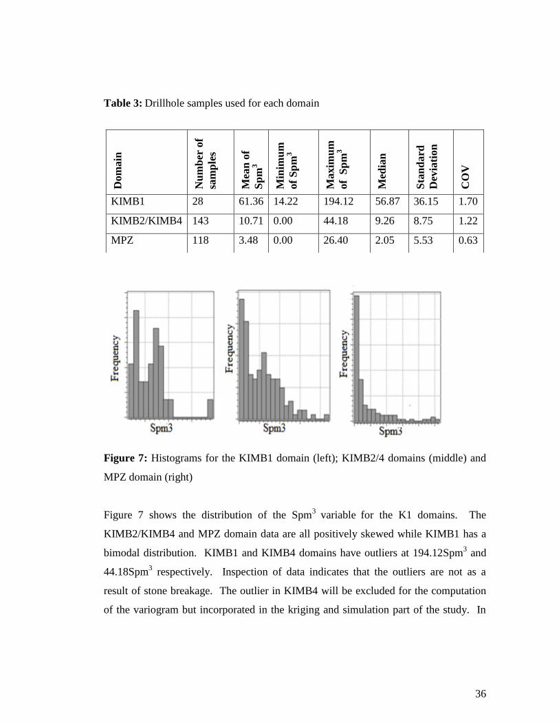
Figure 7 shows the distribution of the Spm3
variable for the K1 domains. The
KIMB2/KIMB4 and MPZ domain data are all positively skewed while KIMB1 has a
bimodal distribution. KIMB1 and KIMB4 domains have outliers at 194.12Spm3 and
44.18Spm3 respectively. Inspection of data indicates that the outliers are not as a
result of stone breakage. The outlier in KIMB4 will be excluded for the computation
of the variogram but incorporated in the kriging and simulation part of the study. In
Dom
ain
Nu
mb
er o
f
sam
ple
s
Mea
n o
f
Sp
m3
Min
imu
m
of
Sp
m3
Maxim
um
of
Sp
m3
Med
ian
Sta
nd
ard
Dev
iati
on
CO
V
KIMB1 28 61.36 14.22 194.12 56.87 36.15 1.70
KIMB2/KIMB4 143 10.71 0.00 44.18 9.26 8.75 1.22
MPZ 118 3.48 0.00 26.40 2.05 5.53 0.63

37
the 2000 model the outliers had a restricted radius of influence applied. In this study
the restricted radius of influence will not be applied.
The outliers cannot be considered as anomalous data as the exploratory data analysis
has sought for and removed or corrected any anomalous data. The high values
typically come from heavy-tailed distributions, where a small number of samples can
be responsible for a large proportion of the metal content or grade in the deposit.
Parker (1991) reported a case where 4 out of 34 samples are responsible for 70% of
the gold content, and 7 out of 34 for 90% of the gold content. He notes, even small
changes in the grade near these assays or the proportion of high-grade material may be
responsible for large differences between estimated and recovered reserves.
Discarding the high grades completely creates a bias. The value of a deposit may just
come from these high grades. In some cases, high grades are deliberately left out with
the idea that it is more rewarding to revise estimates up than down. The problem is
that this may lead to the abandonment of the project if it was a marginal one.
3.2 Data declustering
Geological sampling programs are not entirely spatially random hence the removal of
potential bias or “declustering” the data is vital. The declustering process adjusts the
summary statistics to be representative of the entire area of interest thereby removing
potential bias, for example one area may have clustered sampled points compared to
other portions (Deutsch and Journel, 1998). Since in conditional simulation the
histograms and summary statistics of the conditioning data are an essential foundation
for the accuracy of the resultant model they need to be representative of the volume of
interest. Weights are assigned to each data point based on their proximity to
surrounding data. An example of a declustering method termed cell declustering,
divides the area of interest into regular cells at a given grid spacing. The weight for
each cell, and all data points inside that cell, is calculated as:

38
m t nts n c t m cc c s
The correct cell size is determined by calculating the weights at multiple cell spacings
and then plotting the cell sizes against the mean of the data with the weights applied
(the declustered mean). The final grid size used is the grid size that either minimizes
or maximises the mean. Often, the cell size that is roughly equal to the average
sample spacing is an appropriate choice.
The Murowa data was not declustered in the current study because the samples that
were used were taken at regular intervals of 15 m. The sample lengths of 15 m were
chosen such that between 3 and 30 stones would be recovered given a grade range
between 0.1 and 1 cpt and a sample tonnage of around 3 tonnes. This range of stone
recoveries was recommended as a minimum for the statistical evaluation of grade in
the 2000 evaluation. The sample lengths were kept at a consistent bench depth with
no allowance for likely lithological or grade variations. This was done partly to keep
the sample support consistent throughout the evaluation without the need to composite
the data.
3.3 Variography of the domains of the K1 pipe
Data was read into the SGeMS software from where the variography was performed.
A version of SGeMS which is still under development was obtained from the
developer with additional algorithms that are able to simulate blocks.
The downhole (along the Z axis) semi- variogram of the KIMB2/4 domain
(untransformed data) was first constructed to determine the nugget effect. A 15 m lag
interval was chosen due to the 15 m sampling interval in the downhole direction. A
nugget of 10 Spm3 and a range of 53 m were modelled (Figure 8).
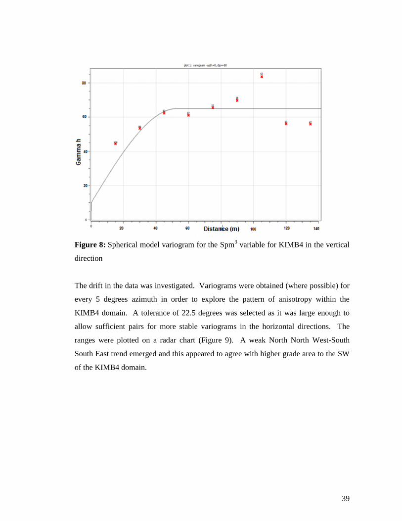
39
Figure 8: Spherical model variogram for the Spm3 variable for KIMB4 in the vertical
direction
The drift in the data was investigated. Variograms were obtained (where possible) for
every 5 degrees azimuth in order to explore the pattern of anisotropy within the
KIMB4 domain. A tolerance of 22.5 degrees was selected as it was large enough to
allow sufficient pairs for more stable variograms in the horizontal directions. The
ranges were plotted on a radar chart (Figure 9). A weak North North West-South
South East trend emerged and this appeared to agree with higher grade area to the SW
of the KIMB4 domain.

40
Figure 9: Radar chart of Horizontal variogram ranges of the KIMB4 domain
The directional horizontal variograms were investigated using both spherical and
exponential variogram type models. The experimental variograms are presented in
Appendix II. However the spherical type model fitted much more accurately to the
omni-directional variogram. The omni-directional variogram also defined a better
structure than the horizontal variograms and was therefore used during the estimation.
A spherical omni-directional variogram for the MPZ domain also defined a better
structure than the other directional variograms and therefore used as the final
variogram. The resultant semi-variograms of the KIMB4 and MPZ obtained are
summarised in Table 4 and the KIMB4 variogram is shown in Figure 10. KIMB1
domain was not investigated due to the small number of samples and therefore
insufficient pairs in some directional variograms.

41
Figure 10: KIMB4 omni- directional spherical variogram model for the Spm3 variable
Table 4: The omni-directional semi variograms models from KIMB2/4 and MPZ
domains
Domain
Variogram Type
C0
C1
Range Azimuth/Dip
Omni
directional
KIMB2/4 Semi variogram
(spherical)
10 75 105 00/00
MPZ Semi Variogram
(Spherical)
12 25 105 00/00

42
4 GEOSTATISTICAL ANALYSIS OF THE SPM3 VARIABLE OF THE
KIMB4 DOMAIN
Numerous authorities have discussed the fundamentals of geostatistics in detail (e.g.
Deutsch and Journel, 1998 and Isaaks and Srivastava, 1989). Geostatistical
estimation can be defined as the prediction of the value of an attribute at a location at
which it is unknown from measured values of that characteristic at a number of known
locations through a function defining the spatial correlation between values (Dohm,
2010). Both kriging and simulations have had much theoretical development and are
well described in most geostatistical literature and are mostly used in the mining
industry.
Most geostatistical methods rely on the assumptions of stationarity, which is seen as
the decision to pool data within a given area or domain. Deutsch and Journel (1998)
state the importance of making proper decisions about stationarity as they are critical
for the representativeness and reliability of the geostatistical tools used. Samples from
geozones or domains of similar geology be it rock type, chemical characteristic,
structure, grade are grouped together. Dividing a dataset into areas that are acceptable
with regards to stationarity is therefore essential in geostatistics.
4.1 Ordinary Kriging
Ordinary Kriging (OK) was developed by Matheron in the early 1960s based on the
Master's thesis of Danie G. Krige, the pioneering plotter of distance-weighted average
gold grades at the Witwatersrand reef complex in South Africa. Ordinary Kriging is
the form of kriging used mostly because it works under simple stationarity
assumptions and does not require knowledge of the mean (Chilès and Delfiner, 2012).
A good estimator will be unbiased, that is, on average the estimated values will equal
the unknown values and the estimation errors (Z-Z*) will be as small as possible.

43
In kriging (and simulation), the search volume or kriging neighbourhood can have
significant impact on the outcome of the estimates and therefore a suitable
neighbourhood has to be determined. Most criteria discussed by a number of authors
e.g. Vann etal, (2003) to consider when evaluating a particular kriging neighbourhood
include the following:
• Slope of regression of the data values vs. the estimates (Z/Z*)
• Weight of the mean in simple kriging
• The distribution of kriging weights
• Variance of the estimator Z*
• Percentage blocks filled
• Mean of the estimate vs. mean of the sample data
• The proportion of negative weights is kept relatively low
In the current study, a number of kriging neighbourhoods were evaluated and a
neighbourhood of 120m, 225m and 15m in X, Y, Z directions was used.
Local point and block estimates of the variable were obtained using OK (unknown
mean) and the variogram model shown in Figure 10. The blocks in the KIMB4
domain were discretised into 5x5x1 based on the stabilisation of the estimation
variance at 5x5x1 in a discretisation test (Figure 11).

44
Figure 11: Discretisation test used to determine the optimal block discretisation of
5x5x1 for the KIMB4 domain
Table 5: Table showing a comparison of the estimates and actual values of the KIMB4
Estimate Actual
Sample
Value
Average
Estimated
Average
Actual
Sample
Value
Standard
Deviation
Estimated
Standard
Deviation
Point Kriging 10.71 10.95 8.75 9.4
Block Kriging 10.71 11.38 8.75 7.33

45
0
5
10
15
20
25
30
35
40
45
50
0 5 10 15 20 25 30
Ra
w S
pm
3
Estimate Spm3
-8
-7
-6
-5
-4
-3
-2
-1
0
1
2
3
4
5
0 5 10 15 20 25 30
Z*
-Z/S
td D
ev
Spm3 Block Estimates
The point and block estimates are very close (Table 5). However the estimated
standard deviations differ with the point estimate being larger than the block estimate.
This reduction of the standard deviation in the block estimate is expected in
estimations such as kriging where the variance decreases with the size and volume of
the unit being considered, in this case drillhole sample support versus block support.
Figure 12: Cross validation of the Spm3 estimates from the KIMB4 domain

46
Validation of the block estimates was performed using a combination of the Inverse
Power Distance (IPD) estimates and a comparison of bench (15m interval) averaged
estimates and sample data, comparison of mean of the estimate and mean of the
sample data, (already seen from Table 5) and cross-validations shown in Figure 12. A
total of 90% of the estimates tested as robust. The non-robust estimates are shown in
red.
Both Simple Kriging (SK) and OK can be used as basis for conditional simulation.
However according to strict stationarity theory, SK should be applied to Gaussian or
NS transforms. The conditional simulation in this study will use SK.
4.2 Normal Scores variography of the KIMB4 domain
A NS transformation was performed in preparation for the simulation of the Spm3
variable but also to compare point kriging results from this transformed data and the
untransformed data. Normally, kriging data with skewed distributions can result in
spurious estimates and such data would be transformed using transformations such as
the Gaussian transformation into a normal distribution before variography is
performed. This would then require back transformation to the original units. The
main drawback of using kriging in NS or gaussian space is that the change of support
is not always straightforward. Ortiz and Deutsch (2003) illustrated how the mean can
be back-calculated using numerical integration. The illustration used considers that a
spatially distributed dataset z (uα), α = 1,..., n is declustered. The cumulative
frequency (F(z)) is read from the original distribution and the value yi of a standard
normal distribution, corresponding to that cumulative frequency (G(y)) is assigned to
the data location and a normal score transformation is performed, generating the
normal/gaussian values y(uα), α = 1, ..., n. This is illustrated in Figure 13.

47
Figure 13: The normal score transformation for data zi. At the bottom is the
anamorphosis function. Sourced from Ortiz and Deutsch (2003)
Under the Gaussian assumption, the shape of the conditional distribution is Gaussian
and therefore the full conditional distribution in the original units of the variable can
be retrieved by back calculating the z values for several quantiles. This is illustrated in
Figure 14. In this illustration nine deciles of the distribution, y1,..., y9, are back-
transformed (top) and the corresponding values, z1, ..., z9, are used to calculate the
mean. The full distribution in original units can be retrieved in the same manner. The
estimation variances can also be back-transformed to express the local uncertainty but
this requires additional processing. Deutsch and Lyster (2004) investigated the impact
of the additional processing on back-transformed kriging means and variances using a
program called PostMG developed within GSLIB. PostMG was specifically written to
perform the back transform of kriged (multi)gaussian output. What became apparent

48
was that the PostMG did not improve the quality of kriged estimated mean but
returned the correct variances for each estimated point. The kriged normal scores
variances were properly back-transformed and could be used more reliably to analyse
uncertainty.
Figure 14: Calculation of the mean by numerical integration. Sourced from Oritz and
Deutsch (2003)
The Spm3 data was transformed using the Histogram transformation algorithm in
SGeMS and the resultant data distribution and parameters shown in Figure 15 (bottom

49
right). It is vital that the standard normal simulations be back-transformed to match
the histogram of the sample values after they are generated.
Figure 15: Normal scores transformation process and resultant parameters of the
KIMB4 Spm3 variable
The transformation also involves extrapolation of the tails of the distribution, for
which the user sets the minimum and maximum allowed limits for the back-
transformed values. 0 and 45 Spm3 were used for the KIMB4 domain as these values
were considered close to the limits of the actual data.
50
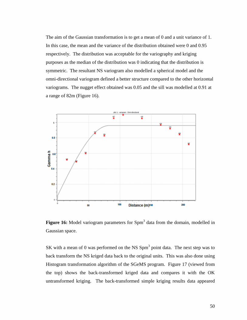
The aim of the Gaussian transformation is to get a mean of 0 and a unit variance of 1.
In this case, the mean and the variance of the distribution obtained were 0 and 0.95
respectively. The distribution was acceptable for the variography and kriging
purposes as the median of the distribution was 0 indicating that the distribution is
symmetric. The resultant NS variogram also modelled a spherical model and the
omni-directional variogram defined a better structure compared to the other horizontal
variograms. The nugget effect obtained was 0.05 and the sill was modelled at 0.91 at
a range of 82m (Figure 16).
Figure 16: Model variogram parameters for Spm3 data from the domain, modelled in
Gaussian space.
SK with a mean of 0 was performed on the NS Spm3 point data. The next step was to
back transform the NS kriged data back to the original units. This was also done using
Histogram transformation algorithm of the SGeMS program. Figure 17 (viewed from
the top) shows the back-transformed kriged data and compares it with the OK
untransformed kriging. The back-transformed simple kriging results data appeared

51
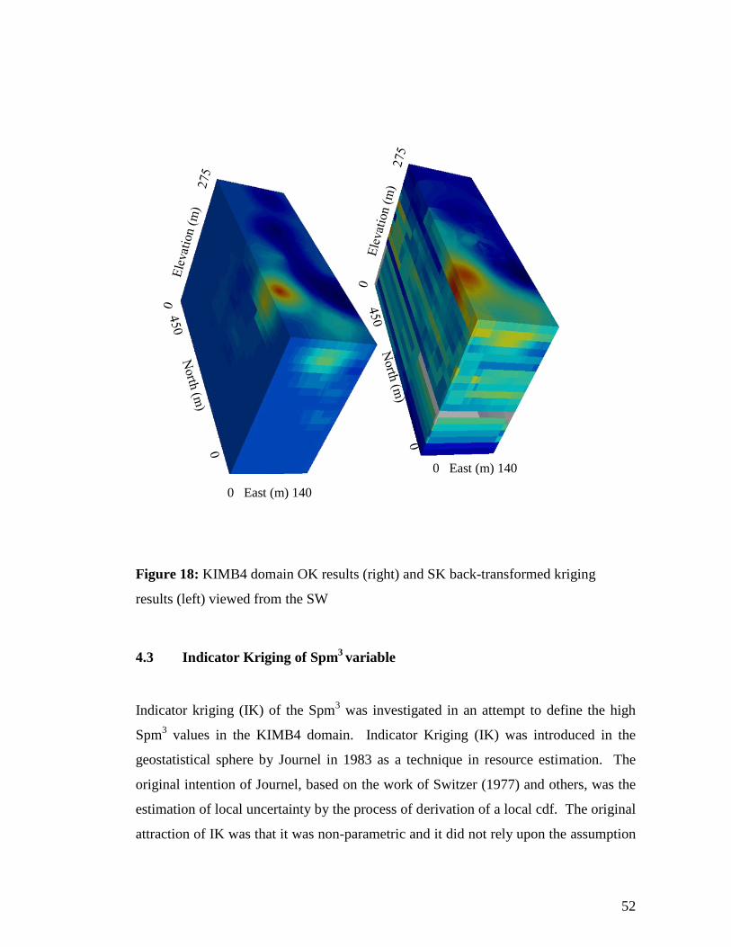
less smoothed compared to the OK results. The high grade area in the South West
using NS is more much more-well defined forming a North West- South East linear
feature. Figure 18 attempts to show the extent of the high grade area at depth. The
high Spm3 estimate seemed to be confined close to the surface (about 30m) and does
not continue at depth where the region is generally poorly sampled. At this stage
however, the back- transformation returned an average Spm3 average which is
comparable to the OK mean. It is therefore the author’s opinion that the back-
transformation in SGeMS is able to return the back-transformed mean. The
performance of the algorithm in returning the corresponding back-transformed
variances that can be used for accessing uncertainty will be investigated and discussed
in Section 6.
Figure 17: Comparison of untransformed OK (left) and gaussian (NS) back-
transformed kriging map outputs (right)
52
Figure 18: KIMB4 domain OK results (right) and SK back-transformed kriging
results (left) viewed from the SW
4.3 Indicator Kriging of Spm3
variable
Indicator kriging (IK) of the Spm3 was investigated in an attempt to define the high
Spm3 values in the KIMB4 domain. Indicator Kriging (IK) was introduced in the
geostatistical sphere by Journel in 1983 as a technique in resource estimation. The
original intention of Journel, based on the work of Switzer (1977) and others, was the
estimation of local uncertainty by the process of derivation of a local cdf. The original
attraction of IK was that it was non-parametric and it did not rely upon the assumption
0 East (m) 140
0 East (m) 140

53
of a particular distribution model for its results. IK has grown to become one of the
most widely-used algorithms and it is the prime non-linear geostatistical technique
used today in the minerals industry (Blackney and Glacken, 1998). The essence of the
indicator approach is the binomial coding of data into either 1 or 0 depending upon its
relationship to a cut-off value, zk. For a given value z(x),
= { t s
Then, the semivariogram (ɣ (h)) is used to express the spatial structure of indicator
codes, written as follows:
ɣ (h) =
∑ [ ]
h is the distance between locations xi and xi + h and N(h) is the number of pairs (xi, xi
+ h). The ccdf at the unsampled location at x can be obtained by the IK estimator:
F[ | n ] =
=∑
where are the weights and (n) is the set of n observed data points used.
This is a non-linear transformation of the data value, into either a 1 or a 0. Values
which are much greater than a given cut-off, zk, will receive the same indicator value
as those values which are only slightly greater than that cut-off. Hence indicator
transformation of data can be an effective way of limiting the effect of very high
values. SK or OK of a set of indicator-transformed values will provide a resultant
value between 0 and 1 for each point estimate. This is in effect an estimate of the

54
0
10
20
30
40
50
60
70
80
90
100
0 2 4 6 8 10 12 14 16 18 20 22 24 26 28 30 32 34 36 38 40 42
Pro
po
rtio
n a
bo
ve
cu
t-o
ff (
%)
Cut-Off Grade (Spm3)
Cut-off vs. proportion above cut-off
proportion of the values in the neighbourhood which are greater than the indicator or
threshold value.
The transformations are also able to derive local distributions of uncertainty which
lead to a practical estimate of resources above a range of cut-off grades. These
estimates called ‘recoverable resources’, while representing the correct support for
mining still need to be subjected to the reserve process. On the downside, the IK
method has since attracted considerable debate as to whether or not it is a valid
technique. A particular issue is that indicator variograms tend towards pure nugget
effect as the threshold increases. Other problems with datasets for example change of
sample support (Chilès and Delfiner, 2012), or clustering of data (Isaaks and
Srivastava., 1989) can also prevent the application of indicator kriging. However
these problems are not present in the KIMB4 data set.
In order to get an indication of cut-off values that define high and low Spm3 values in
KIMB4, a number of different cut-off values of Spm3 were investigated. Estimates
were performed using the 12 Spm3 cut-off and they are presented in Figure 19 and the
rest are shown in Appendix III.

55
Figure 19: Relationship between various cut-offs of Spm3 and the proportion above
cut-off (top) and the model indicator variogram at a cut-off of 12 Spm3.
Figure 20: Kriged map of Spm3 >12 viewed from the top, as well as the block model
of the KIMB4 domain.
0 East (m) 140

56
Figure 20 shows the kriged map of Spm3 >12 viewed from the top as well as the block
model of the KIMB4 domain.

57
5 CONDITIONAL SIMULATION OF THE SPM3 VARIABLE OF THE
KIMB4 DOMAIN
The direct block simulation (DBSIM) method has been proposed as an alternative to
conventional SGS. The method considerably reduces computational time. DBSIM
simulates the internal points of each block and when the simulated block is calculated
the point values are discarded. The simulated block value is then added to the
conditioning dataset. To integrate the block support conditioning data the algorithm
has been developed in terms of a joint simulation, where the second variable relates to
the block values sequentially derived through the simulation process. The algorithm
simulates several hundreds of blocks per second and is considerably faster than any
point conditional simulation combined with re-blocking. Furthermore
Dimitrakopoulos, et al., (2002), show that in addition being substantially faster and
more efficient in terms of computing requirements, the DBSIM method is equally
reliable in terms of reproduction of the sample statistics.
However because simulating points using SGS with the aim to re-block so as to yield a
block value had the added advantage of getting the point estimates as well, for the
current study this approach was preferred over the block simulation method. The
approach was proposed by Deutsch and Journel in the 1990s and was accepted by
several authorities (e,g. Dimitrakopolous, et al., 2002). The block simulations were
therefore done using point simulations followed by averaging to the mining block
sizes (re-blocking).
5.1 The Theory of Sequential Gaussian Simulation
Like kriging the theory of simulations has been documented by authors such as
Deutsch and Journel (1998) and Chilès and Delfiner (2012). While this technique
ensures reproduction of spatial data, it is also founded on a very strong assumption of
58
stationarity just like kriging where in particular, the mean is assumed to be the same at
every location in the field. Domains are generally used to constrain fields with a
common mean; yet, when no hard boundary between varying means exists, such as
when there is a continuous trend in data, the stationarity assumption however cannot
be maintained.
Kriging and conditional simulation differ fundamentally although differences between
them can be subtle at times. The main differences between the two are that:
The aim of kriging is to provide the best linear unbiased estimate (BLUE) of
the variable, without consideration of the spatial statistics of all the estimates
collectively. The focus is on local accuracy as opposed to spatial continuity.
(Deutsch and Journel, 1998).
Conditional simulation presents a more accurate picture of the true variance
within a dataset compared to kriging. Simulations in general focuses on more
correct spatial continuity
The theoretical explanation of the mathematical fundamental principles of the SGS
technique to be briefly discussed in this section was taken from Delfiner and Chiles
(2012). The theory considers as a vector-valued random variable Z (Z1, Z
2,...,Z
N) for
which a realization of the sub vector (Z1,Z
2,...,Z
M) is known and equal to (z
1,z2,..., z
M)
(0<M<N). The distribution of the vector Z conditional on Zi = zi, i=1, 2,...,M, can be
factorized in the form:
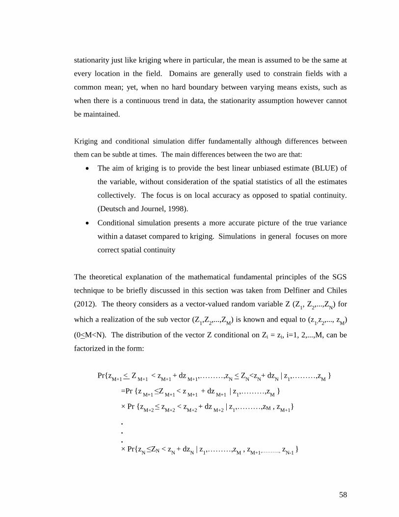
Pr{zM+1 < Z
M+1 < zM+1 + dz M+1
,………,zN < Z
N<z
N+ dz
N | z
1,………,z
M }
=Pr {z M+1 ≤Z
M+1 < z M+1 + dz M+1 | z1
,………,zM
}
× Pr {zM+2
≤ zM+2 < z
M+2 + dz M+2
| z1,………,zM , z
M+1}
.
.
.
× Pr{zN ≤ZN < z
N + dzN | z
1,………,z
M , z
M+1,………., zN-1 }

59
The vector Z is sequentially simulated by randomly selecting Zi from the conditional
distribution Pr{Zi<zi| zi,……..,zi-1) for i = M+1,……,N and including the outcome Zi
in the conditioning dataset for the next step. In the case of a Gaussian random vector,
the conditional probabilities can be calculated.
If the above method is applied to the simulation of a Gaussian random function the
simulation is SGS. If the Gaussian RF has a known mean, the conditional distribution
of Zi therefore is Gaussian, with mean zi and variance
ki. Here Zi is the SK of Zi
from {Zi:j<i}, and
ki is the associated kriging variance.
The sequences of steps to generate an SGS are as follows:
Transform data to Gaussian space.
Compute and model the variogram of the transformed data.
Define a random path that passes through each node of the grid
representing the deposit.
Krige the normalised value at the selected node and obtain the kriged value
The simulated value could also be obtained by drawing from a normal
distribution using the kriged estimate and the kriging variance as the mean
and variance respectively.
Add the new simulated point to the conditioning data set, move to the next
node and repeat the kriging and random sampling of the resultant
The SGS method has several advantages which include:
Sequential simulations are easy to understand
A variety of algorithms exist for its implementation
Conditioning and simulations are part of an integrated process
Anisotropies are handled automatically
Applicable to any covariance function

60
5.1.1 Validation of the simulations
Several aspects that can be considered in order to evaluate the performance of the
simulations include:
Gaussian statistics: How close are the Gaussian mean and variance to zero and
one?
Raw univariate Statistics: How close are the back-transformed mean and
variance of the simulations to the original data?
Histograms: How well do the histograms of the variable reproduce the
histogram of the drillhole data?
Correlation coefficients: How well do the simulation reproduce the correlation
coefficient of the drillhole data?
Scatterplots: Are the scatterplots of the simulations comparable to those of the
drillhole data?
Variograms: Are the experimental variograms of the simulations comparable to
those of original data?
Spatial patterns: Do the graphical images of the simulations represent
geologically plausible spatial patterns? Are there any obvious visual artifacts or
errors such as elevated grades?
Space of uncertainty: Could the true grades be outside the range of the grades
simulated?
5.2 The application of sequential gaussian simulation to the Spm3 variable
This section will produce realisations of the Spm3 variable on a point support scale using
the sequential gaussian simulation method. To incorporate the change of support, the
blocks were discretised into a point scale grid and the nodes then simulated by point
simulation. The point simulations were then averaged out on block scales using the
Block Upscaling (Block Averages) Menu.

61
This approach was preferred for this study as it offers two advantages:
Both the point and the block simulations are obtained. For example in
simulation of mining methods, an additional reconnaissance survey (e.g. pre-
mining drill-holes) and mining blocks (selection units) can be simulated at the
same time.
It is very fast to generate a simulation for a new block size, or simulate blocks
of variable dimension.
The KIMB4 domain is approximately 140m x 450m x 275m (X, Y, Z). In this study,
the fifty realizations were simulated within the KIMB4 domain by discretising the
mining block into 2.5m x 2.5m x 15m grid per regularised (SMU) block (25m x 25m x
15m) and then simulated by point simulation. This grid size was considered to be
small enough to accommodate SGS, yet is large enough for timely processing and
avoided subsampling as well. The simulation grid required 1 node for each block. The
total number of nodes therefore required for the simulation was thus 184800.
The conditional Sequential Gaussian Simulations generated as part of this study were
performed using the following steps:
Transforming of the raw drill hole data into Gaussian space using the
Histogram Transformation algorithm in SGeMS.
Modelling the variogram using the Gaussian space data using the variogram
module in SGeMS. This and the previous step have already been undertaken in
the kriging using Normal Scores section of the study
Running a total of 50 simulations using the SGS algorithm in SGeMS.
Various authors have used different numbers of realisations to model
uncertainty. Dimitrakopoulos, et al., (2002) considered that 50 realisations
were sufficient for their purposes while Goovaerts (1997) makes reference to
100 realisations.

62
However a balance is required between reducing the number of realisations,
and thus the computing time, without compromising the validity of the
simulated model. To determine the number of realisations that would be
required to obtain a reliable uncertainty model, the number of realisations are
plotted against the progressive mean and progressive coefficient of variation
(COV) (Appendix IV). This approach was adopted from Robin (2006) and 50
realisations were optimal for this case.
Kriging points from the surrounding data at each simulation node using simple
kriging (mean=0 and variance = 0.95)
Back-transformation of the gaussian conditionally simulated values to raw
space.
Verifying the conditional simulation by comparing the variogram of the input
sample data against variograms of individual point simulations and by comparing
the base statistics of the sample data against those of the conditional simulation
and kriged output.
5.2.1 Validation of the Spm3 variable simulation
The following observations were made with regards to the aspects that need to be
considered to validate the simulations
A mean of 0.04 and variance of 0.91 (compared to 0.95 variance of the
Gaussian transformation) was obtained for all the simulations collectively.
The NS histograms statistics were reproduced and Figure 21 show the
cumulative frequency of 10 randomly selected realisations (in blue) compared
to the input data (in red)

63
Figure 21: Cumulative frequency distribution of 10 randomly selected realisations in
NS (in blue) compared to the cumulative frequency of the input data (in red)
The global characteristics also did not vary much between the individual
realisations. The individual back-transformed realisations reproduced the
histograms and frequency distribution of the input sample data (Figure 22 and
Figure 23).
To further compare the global statistics, an approach adopted from De-Vitry
(2010) was adopted. Firstly the mean and variance of the individual
realisations were divided by the mean of the drill hole data and multiplied by
100 to give a ratio. Realisations that have means above 100% are generally
over simulated while those below 100% are under simulated. The ratios of the
means and variances of the realisations produced were calculated for the Spm3
variable. The means were close to 100% while the variances were an average
of 5% above the 100% ratio.

64
Figure 22: The univariate statistical parameters of randomly selected histograms
generated from the Sequential Gaussian simulation of Spm3 compared to those of the
sample data (bottom left).

65
Figure 23: Frequency distribution of 10 randomly selected back-transformed
realisations (in blue) compared to the raw Spm3 data (in red)
Correlation coefficients are an effective summary of how well the simulated
Spm3 variable correlated to the raw drill hole data.
Absolute differences between the correlation coefficients of the realisations
and the correlation coefficients of drillhole data were calculated. The absolute
difference is a measure of how closely the simulations reproduced the drillhole
coefficients. A value close to 0 (zero) is desired and an average of 0.14 was
obtained in this case. Nineteen realisations had these differences above the
0.14 average.
The scatter plot of the correlation coefficients of the realisations and the
correlation coefficients of the drillhole data were generally characterized by a
few outlying points. It was observed that other realisations outside the 19
(above the 0.14 average) had more pronounced outlying points.
The sills of the experimental back- transformed variograms (about 10
randomly selected realisations were used) plotted slightly below that of the
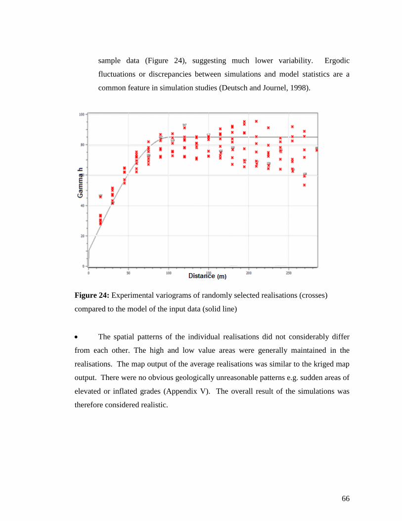
66
sample data (Figure 24), suggesting much lower variability. Ergodic
fluctuations or discrepancies between simulations and model statistics are a
common feature in simulation studies (Deutsch and Journel, 1998).
Figure 24: Experimental variograms of randomly selected realisations (crosses)
compared to the model of the input data (solid line)
The spatial patterns of the individual realisations did not considerably differ
from each other. The high and low value areas were generally maintained in the
realisations. The map output of the average realisations was similar to the kriged map
output. There were no obvious geologically unreasonable patterns e.g. sudden areas of
elevated or inflated grades (Appendix V). The overall result of the simulations was
therefore considered realistic.
67
6 ASSESSING UNCERTAINTY IN THE KIMB4 DOMAIN
Deutsch (2011) devised a workflow to assess uncertainty of variables over an area of
interest using kriging and conditional simulation means and variances. This approach
involves evaluating the kriging means and their associated variances and conditional
means and conditional variances using map outputs to delineate areas of low and high
variances. The conditional kriging variances are able to give a visual indication of
local uncertainty via the conditional variance maps output.
In kriging with the NS data, the kriging variances become data-value dependent unlike
using the original data where the estimates are dependent on the configuration of the
sampling points. Some geostatistical software are equipped with algorithms which can
back-transform the NS kriging estimates back to their original units. The processes
behind the back transformation have been discussed. With the conditional
distributions back in original units, the mean and variance are also back in original
units but they are now dependent on the data values.
While kriging variance map outputs generally show strong dependency on the data
configuration where values are lowest at the data points (regardless of the values) and
increase away, the original units conditional variance show dependency on the data
values. The variances can be uniformly higher in high point value areas or more
uniformly lower in generally lower point value areas. Therefore the conditional
variances are much more trustworthy. These areas are therefore "certain" or are areas
of low uncertainty. There will still be areas where it is not clear whether they are high
or low variance areas. These will be areas where uncertainty is highest.
This approach was used in this study to help delineate areas within the KIMB4 domain
which have surely high and low variance as well as those where it is difficult to tell
and therefore present areas of high uncertainty in the grade estimates.

68
6.1 Measures of uncertainty
A variety of summary statistics and uncertainty measures such as conditional
variances, IQR, Conditional COV (CCOV) and probability intervals can be derived
from the resulting cdf and used to support decision making. The conditional variance
measures the spread of the cdf around its mean value Z*:
ar =∑[ ]2
+1
=1
where:
k=l,...K, are K threshold values discretising the range of variation of z
values
is the mean of the class which in case of a within class
linear interpolation model corresponds to = ( + ) /2
is the expected value of the cdf approximated by the discrete sum:
=∑
+1
=1
[ ]
The conditional coefficient of variation (CCOV) or relative conditional standard
deviation corresponds to the conditional standard deviation divided by the mean. The
CCOV expresses variability as a percentage of the mean, and is calculated as follows:
=√[ ]
2.
The conditional interquartile range (IQR) is defined as the difference between the
upper and the lower quartiles of the normal distribution:

69
=
=
The accompanying realisation map outputs or images from the simulations can also be
visually compared among themselves and against the kriging maps. Spatial features
are deemed to be “certain” if they are present in most of the simulated maps and
“uncertain” if they only appear on relatively few simulated maps. Probability type
information and map outputs are instrumental in establishing the probability of
variables to be above certain thresholds as well as how the distribution of the areas
changes with the different thresholds.
6.2 Point kriging model
The final point kriged model contained back-transformed NS kriging of the Spm3
variable, conditional means and variances, IQR, 0.05, 0.5 and 0.95 quantiles, CCOV
and the probability that the grade would be greater than 0.2ct/t.
Point kriging of the Spm3 variable was done in Section 4 where initially, OK was used
to obtain the estimate of the Spm3. This was followed by SK using normalised Spm
3
values. According to Deutsch (2011), SK with normal scores (NS) with a mean of
zero can be equated to computing a conditional mean and a conditional variance by
solving normal equations. In line with Deutsch's workflow, the variography and
kriging were carried out NS with a mean of 0 and variance of 0.95. The NS kriged
estimates of Spm3 variable were then back-transformed to the original units. The
gaussian values (-2.46 to +2.46) were back-transformed using the Histogram
Transformation algorithms of the SGeMs software. The initial transformation targeted
the raw Spm3 distribution thereby conditioning the estimates to the point distribution.
Using the Post Kriging algorithm of the SGeMS program, the conditional mean and
variances, IQR as well as quantiles, probability of being over or below the mining
grade cut-off were then computed.

70
The back-transformed map output showed slight disparities when compared to the
respective kriged NS conditional map and OK output (Figure 25) but the high Spm3
(>12 Spm3) areas to the South Western edge of the domain remained high, and the low
values elsewhere remaining low in all the three outputs.
Figure 25: Map outputs of back-transformed NS kriging (left) compared to kriging in
NS with mean of zero (middle) and OK (right) showing the high grade area to the
South West of the domain and low grades estimates elsewhere.
The variances, unlike the kriged estimates behaved differently. The variances of the
back-transformed Spm3 values were significantly lower (+11.1 to +21.8) compared to
the OK variances (+17 to +170). The spatial patterns on the map output of the back-
transformed data also looked identical to the variance map output of the NS variance
(Figure 27). However the histogram returned by the back-transformed variances had
an ‘unusual’ distribution which did not mimic that of OK.

71
Figure 26: Back-transformed NS Variance (left) compared to the Kriging variances in
NS with mean of zero (middle) and OK ( right)
The data distribution and kriging showed that there are fairly high values on the SW
margin of the domain and relatively low values elsewhere. The conditional variances
however showed a poor correlation with the Spm3 variable because low variance
values related to both high and low Spm3 values (Figure 27). The unusual distribution
of the back-transformed variance and conditional variance may therefore indicate the
limitation of SGeMS in back transforming NS variances to be used in assessing
uncertainty.
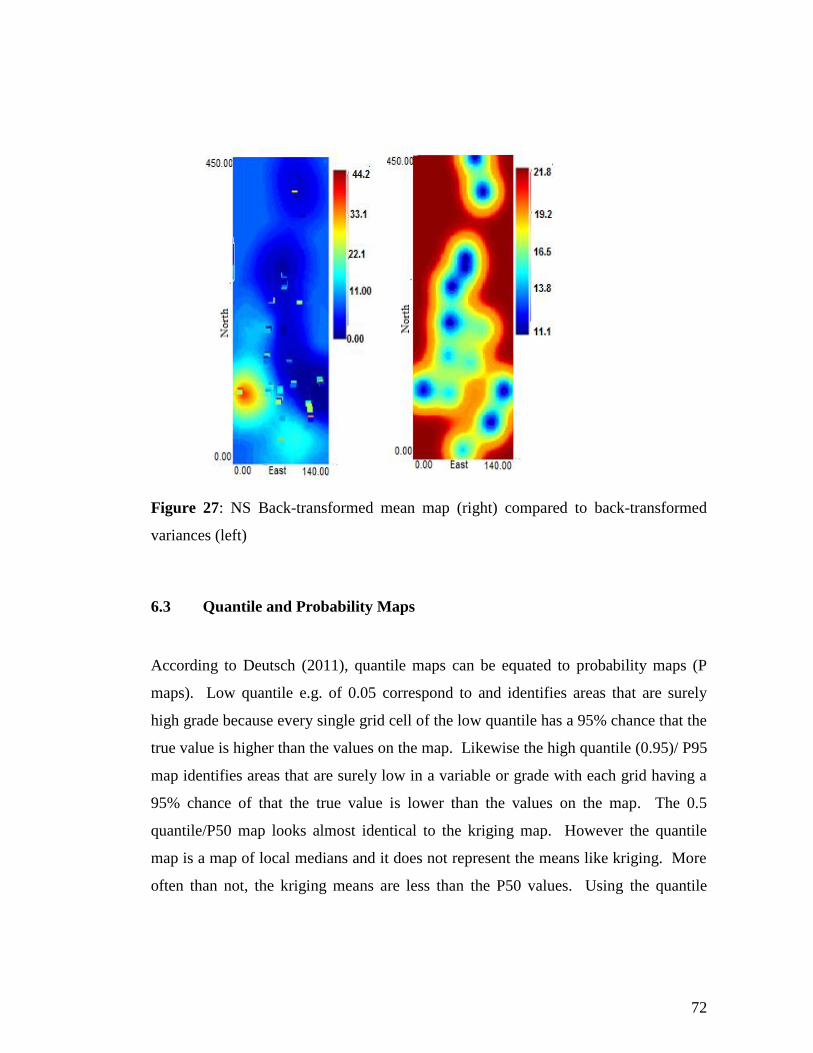
72
Figure 27: NS Back-transformed mean map (right) compared to back-transformed
variances (left)
6.3 Quantile and Probability Maps
According to Deutsch (2011), quantile maps can be equated to probability maps (P
maps). Low quantile e.g. of 0.05 correspond to and identifies areas that are surely
high grade because every single grid cell of the low quantile has a 95% chance that the
true value is higher than the values on the map. Likewise the high quantile (0.95)/ P95
map identifies areas that are surely low in a variable or grade with each grid having a
95% chance of that the true value is lower than the values on the map. The 0.5
quantile/P50 map looks almost identical to the kriging map. However the quantile
map is a map of local medians and it does not represent the means like kriging. More
often than not, the kriging means are less than the P50 values. Using the quantile

73
maps, areas that are surely high and surely low can be flagged and an indication of
uncertainty over an area can be obtained.
Three maps at 0.05, 0.5, and 0.9 quantiles were produced in addition to the NS back-
transformed map and the results are shown in Figure 28.
Figure 28: 0.05 (extreme left), 0.5 (middle left), 0.9 (middle right) probability maps
and NS back-transformed map (extreme right)
The low quantile (0.05) or P5 map corresponds and identifies areas that are surely high
grade because every single grid cell on the P5 map, has a 95% chance that the true
value is higher than the values on the map. Likewise the high quantile map (0.9)/ P90
map identifies areas that are surely low in Spm3 with each grid having a 90% chance
of that the true value is lower than the values on the map.
The quantile map outputs all look very identical when they are compared among
themselves and to the kriging map output. The lowest Spm3 region seems to be
consistently delineated to the east of the domain and these regions continue even at

74
depth while the high value area consistently maps to the SW. Areas where the
estimates are uncertain are rather difficult to delineate. One may suggest the regions
highlighted in a lighter blue to the SE of the high value area but this is also very
subjective.
An attempt to summarise the local distributions of uncertainties by their means and
their variances is presented above. However the measures did not allow for the
assessment of local uncertainty and delineations of the different zones of uncertainty.
Both the conditional mean and variance maps were very identical to the kriging and
kriging variance maps. More importantly the back-transformation of the NS kriging
variances in SGeMS for assessing uncertainty was inadequate. As a result a measure
of variance that is trustworthy and dependable as well as conditional both to data
values and configuration could not be obtained.
6.4 Point Simulation Model
In Section 5 sequential gaussian simulation of the Spm3 variable in the KIMB4
domain was carried out and validated. A total of 50 point realisations were computed
and back-transformed to the original units.
The initial intention of simulation was to take the workflow devised by Oritz and
Deutsch (2003) to block scale by simulating blocks. However because the NS
variances and means did not perform well in determining the local uncertainty within
the KIMB4 domain, the local uncertainty will be investigated using the point
simulations following the same work flow as in the kriged model.
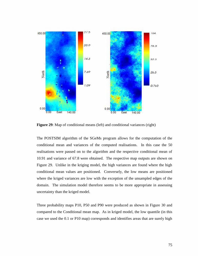
75
Figure 29: Map of conditional means (left) and conditional variances (right)
The POSTSIM algorithm of the SGeMs program allows for the computation of the
conditional mean and variances of the computed realisations. In this case the 50
realisations were passed on to the algorithm and the respective conditional mean of
10.91 and variance of 67.8 were obtained. The respective map outputs are shown on
Figure 29. Unlike in the kriging model, the high variances are found where the high
conditional mean values are positioned. Conversely, the low means are positioned
where the kriged variances are low with the exception of the unsampled edges of the
domain. The simulation model therefore seems to be more appropriate in assessing
uncertainty than the kriged model.
Three probability maps P10, P50 and P90 were produced as shown in Figure 30 and
compared to the Conditional mean map. As in kriged model, the low quantile (in this
case we used the 0.1 or P10 map) corresponds and identifies areas that are surely high
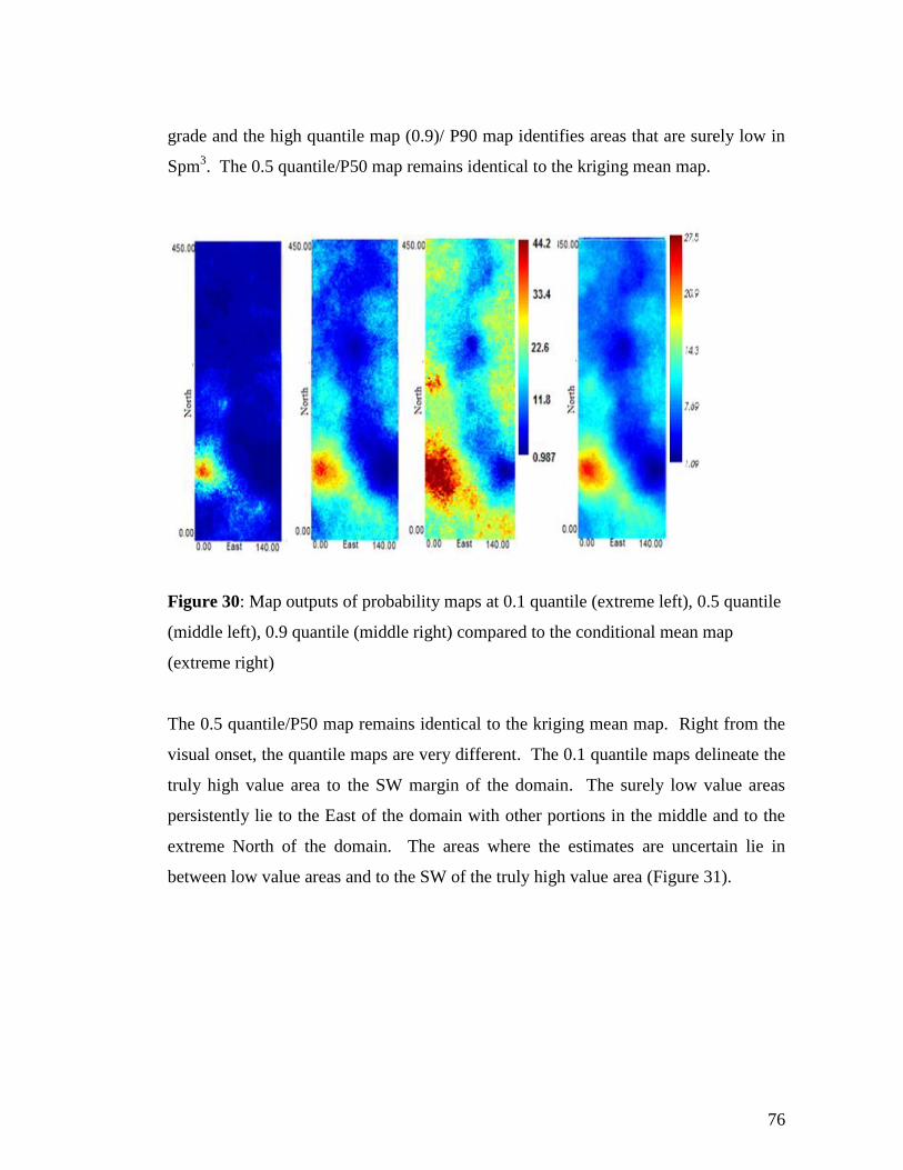
76
grade and the high quantile map (0.9)/ P90 map identifies areas that are surely low in
Spm3. The 0.5 quantile/P50 map remains identical to the kriging mean map.
Figure 30: Map outputs of probability maps at 0.1 quantile (extreme left), 0.5 quantile
(middle left), 0.9 quantile (middle right) compared to the conditional mean map
(extreme right)
The 0.5 quantile/P50 map remains identical to the kriging mean map. Right from the
visual onset, the quantile maps are very different. The 0.1 quantile maps delineate the
truly high value area to the SW margin of the domain. The surely low value areas
persistently lie to the East of the domain with other portions in the middle and to the
extreme North of the domain. The areas where the estimates are uncertain lie in
between low value areas and to the SW of the truly high value area (Figure 31).

77
Figure 31: P10 and P90 maps flagging areas that are surely high (right) and areas that
are surely low in Spm3 estimates (left).
The economic cut-off grade in K1 is 0.2ct/t. The equivalent Spm3 value can be easily
determined since the MSS and density are known (0.0767ct/stn and 2.64t/m3
respectively). This was worked out to be 6.84Spm3. The probability of the grade
being above 6.84Spm3 was investigated and Figure 32 shows the model of the
probability of the grade being above 6.84Spm3. The SW region still has the highest
probability of being above the cut-off grade while the portion to the east which
coincides with the surely low Spm3 area has the lowest and intermediate values in
between.

78
Figure 32: Probability of Spm3 values above 0.2ct/t cut-off.
The interquartile range (IQR) is a relative measure and as such does not use the mean
as the centre of the distribution. This measure ignores the internal distribution of
probability grade, leading to over representing uncertainty. Therefore it was not
considered for this study.
6.5 Presentation of the block model
The block simulations were obtained from point scale realisations averaged into
blocks (25m x 25m x 15m). The final model contained fields for 50 grade block
average realisations, conditional means and variances, 0.05, 0.5, 0.95 quantiles,
Coefficient of Variation and Probability that the grade would be greater than 0.2cpt/t.

79
The univariate statistical parameters generated from the block simulations are
illustrated in Figure 33 and compares against those of the sample data and the kriged
output.
Figure 33: Comparison of univariate statistical parameters of the Spm3 sample data
(top left) against those of the ordinary kriged estimates (top right) and mean of the
simulations (bottom left). The output from the kriging and simulation is also compared
using a quantile-quantile plot (bottom right) where ordinary kriged estimates are
plotted on the X-axis and the Conditional mean of the simulations on the Y-axis.

80
The univariate statistics from the kriging and the average of the simulations are
similar. This is also evident when examining a quantile-quantile plot showing the
output from the kriging and the mean of the simulations. Figure 34 shows map output
from the different techniques used to model the variability and estimate the Spm3
variable of the KIMB4 domain. The angled view attempted to capture and show the
variability in this unit.
Figure 34: Output from the different techniques generated by Kriging (left), SGS
(middle) and indicator kriging results (Prob Z*>12) right
The 50 realisations were passed on to the POSTSIM algorithm and the respective
conditional mean of 10.78Spm3 and variance of 44.73Spm
3 were obtained. The
respective map outputs are shown on Figure 35. The high conditional means and
variances for the block simulations remain confined to the South West of the domain.
The variances remain fairly low elsewhere besides the unsampled edges of the domain.
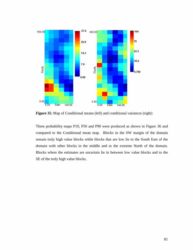
81
Figure 35: Map of Conditional means (left) and conditional variances (right)
Three probability maps P10, P50 and P90 were produced as shown in Figure 36 and
compared to the Conditional mean map. Blocks in the SW margin of the domain
remain truly high value blocks while blocks that are low lie to the South East of the
domain with other blocks in the middle and to the extreme North of the domain.
Blocks where the estimates are uncertain lie in between low value blocks and to the
SE of the truly high value blocks.
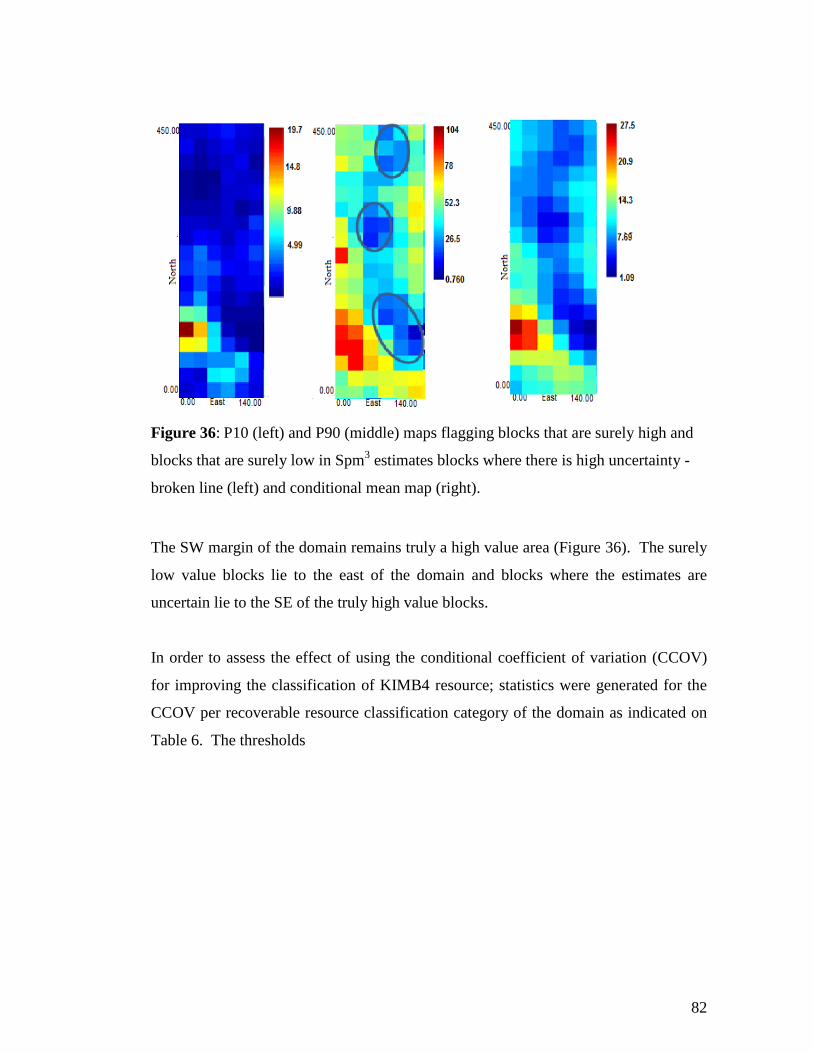
82
Figure 36: P10 (left) and P90 (middle) maps flagging blocks that are surely high and
blocks that are surely low in Spm3 estimates blocks where there is high uncertainty -
broken line (left) and conditional mean map (right).
The SW margin of the domain remains truly a high value area (Figure 36). The surely
low value blocks lie to the east of the domain and blocks where the estimates are
uncertain lie to the SE of the truly high value blocks.
In order to assess the effect of using the conditional coefficient of variation (CCOV)
for improving the classification of KIMB4 resource; statistics were generated for the
CCOV per recoverable resource classification category of the domain as indicated on
Table 6. The thresholds

83
Table 6: Base statistics for CCOV and classification category
Classification CCOV Number of
blocks
% of blocks
Measured 0-2 248 0.12
Indicated 2-4 651 0.317
Inferred 4-8.18 1153 0.561
Figure 37: Block coefficient of variation and resource classification
The dark blue blocks coincide with drillhole points and it is evident that zones of high
confidence (low uncertainty) correspond well with these points, while zones of high
uncertainty correspond with zones that have been insufficiently sampled (Figure 37).
Colouring the simulation model on CCOV will allow for the targeting of specific
zones of highest CCOV and place lower importance on zones with lowest CCOV. In
0-2
2-4
4-8.18

84
this way expenditure on future drilling programmes would thus be optimised to gain
maximum benefit.
The decision to allocate blocks to Inferred, Indicated or Measured resource category at
Murowa remains the responsibility of the competent person. However, using the
CCOV as a measure provides a good, semi quantitative method to use as an aid, which
with similar measures on other variables will make quantitative classification possible.
The coefficient of variation seems to provide a reliable indication of uncertainty in the
simulated grade and is perhaps a more reliable tool for confirming, or even improving,
the classification within the KIMB4. Furthermore, it perhaps is the best tool to direct
drilling programmes in zones that require additional sample information.
This resource classification criterion is based on the uncertainty measures derived
from the cdf of each block in the resource model. The criterion requires the selection
of a threshold value that reflects the error tolerance that is acceptable for the block
estimate. Therefore for given thresholds, the KIMB4 block can be classified at a
Measured, Indicated or Inferred level of confidence depending on whether the CCOV
is less than or greater than the thresholds. The thresholds are user-defined and in this
case the thresholds values ranging from 0 to 2, 2-4 and 4-8.18 were used. In Figure
37 the darker blue coloured blocks representing low CCOV values have been
classified at a Measured resource category while the pale blue blocks are Indicated and
the pales greens and yellows are Inferred.
KIMB4 domain’s CCOV values have highlighted the potential to convert Indicated
material to a Measured status. This is particularly applicable to the central zones
where the classification by T&I may have been too stringent. The Murowa Mine has
not been supplied with this uncertainty model to assist with the planning of additional
drilling aimed at converting Indicated material to Measured status.

85
Figure 38: Proposed LD holes (pink) and P10 and P90 maps flagging blocks that are
surely high and blocks that are surely low in Spm3 estimates and blocks where there is
high uncertainty -broken line (middle and right). The magenta line outlines the KIMB
domains, the yellow line- weathering and the blue the MPZ.
However some drilling to define the resource at depth has been proposed in 2010. A
total of eight holes i.e. 5 x 300 m and 3 x 250 m LDRC holes were proposed to
confirm the measured resource at K1. Generally, the results of the uncertainty model
are not too removed from the proposed holes (Figure 38).

86
7 DISCUSSION
Flagging high and low value areas is essential in making decisions which areas need
additional drilling. These areas are where the uncertainty is highest. In the K1
kimberlite one of the issues that has been raised before was the concern over the
relatively low density of the drilling and relatively small number of samples used in
the evaluation of the K1 kimberlite particularly after the deficit in the reconciliation of
2009. The KIMB4 domain being the most voluminous of the other domains, carries
the bulk of the resource and it is vital to establish where additional drilling can be done
in order to increase the confidence of the estimates.
Figure 39: Post plots of Spm3 values on the geological model in relation to the areas
of high and low uncertainty and resource classification based on COV.
Referring to the post plot in Figure 39 (right), the surely high value area is based on a
single drill hole with high value samples, while SW trending high uncertainty area
seems to have a number of drill-holes but closer under scrutiny, it becomes clear the

87
drill holes are rather widely spaced and the drilling density can potentially be
increased. The area to the north of the high value sample also has a paucity of drill
holes. Drilling density can be increased in these areas.
Of equal interest to delineating areas of high and low uncertainty in grade estimates
would be quantifying the uncertainty. Uncertainty around estimates such as grades in
a deposit can be quantified on a variety of scales such as over regions that represent
set production periods, mining units (SMUs and benches), or over the entire pipe
(Harrison et al 2009). One way of quantifying the risk associated with such estimates
is using the range of grades calculated from the realisations at a particular scale. The
mean grade of each realization at that scale is calculated, realizations are ranked and
ranges of uncertainty can be calculated at preferred confidence limits that can be
generated around the mean of the realisations. In this way high and low estimates can
also be obtained for mine design or pit optimisation.
Uncertainty ranges for the KIMB4 domain were investigated at a 15 m bench scale
using the block model. Twenty realisations were selected and their means calculated
per 15m bench. 15% limits about the mean were selected as they define the limit of
acceptable variability for an Indicated resource status (Figure 40). The 15% limits
were exceeded for a considerable number of the benches although it becomes worse
from about the 12th
bench (555m).

88
Figure 40: Comparison of the output of nineteen individual conditional simulations.
The ±15% envelope about the mean is shown as a reference.
This increased noise at depth seems to be associated with the paucity of sample data
over the last few benches (Appendix V11). This is consistent with the T&I
classification in 2009 where the resource above 545m was classified in the Indicated
Category and below as Mineral Inventory.
Figure 41 shows the mean conditionally simulated Spm3 per bench (representing all
the realisations) along with the 95% confidence limits. This is compared with kriging.
The conditional mean is consistently slightly lower than the kriging although the two
estimates compare very well throughout all the benches. Both the kriging and the
mean of the simulations are also remarkably constrained within the ±15% envelope
about the mean even at depth. Another observation is the elevated average Spm3
values between benches 13 and 14 that are followed by a steep decrease. The maps
comparing kriging with realisations are shown in Appendix VII.
0
2
4
6
8
10
12
14
16
18
20
22
24
0 1 2 3 4 5 6 7 8 9 10 11 12 13 14 15 16 17 18
Sp
m3
Bench Number
Block Model Ranges by Bench Real0
Real2
Real10
Real12
Real14
Real16
Real18
Real20
Real22
Real24
Real26
Real28
Real30
Real32
Real34
Real36
Real38
Real40
Real42
-15%
15%

89
7
8
9
10
11
12
13
14
0 1 2 3 4 5 6 7 8 9 10 11 12 13 14 15 16 17 18
Sp
m3
Bench Number
Simulated Conditional Mean Spm3 per Bench
Cond Mean
15%
-15%
Block Krig
Figure 41: Spm3 Conditional simulated mean per bench along with the 95%
confidence limits.

90
8 CONCLUSIONS AND RECOMMENDATIONS
The KIMB4 domain of the K1 pipe carries the bulk of the resource and therefore the
greatest risk with respect to the grade estimates. The poor grade reconciliation of 2009
compared to the predicted resource model grade necessitated the need to investigate
the geological model and grade estimates and provide an indication of uncertainty
around the grade in this unit.
Both the practices of kriging (to a lesser extent) and simulations via conditional
means, variances, and CCOV were able to provide measures and indication of
uncertainty in the estimates in the KIMB4 domain. Areas of high uncertainty could be
delineated and these areas can be targeted for additional drilling to increase the
confidence and reduce the uncertainty in the estimates. The paucity of sample data
coupled with increased uncertainty in the estimates from about 545m was indicated.
Having an accurate assessment of uncertainty arising from grade variability in the ore
reserve allows risk in a mining project to be quantified and considered in decision-
making processes. This knowledge adds value to a project before the ore reserve is
depleted and before development capital is committed to the project. Although basic,
the uncertainty-based diamond grade models presented in this study are consistent
with standard geostatistical modelling practices. They take into account a variety of
additional factors including global statistics, the representative histogram, and the
model variogram. Of the measures evaluated the CCOV provided a good measure to
use for resource classification and although the method remains semi-quantitative it
was possible to use a CCOV value to assign resource categories in this unit.
The quantification of uncertainty and risk also has major implications for open-pit
design and production scheduling as it relates to the management of cash flows which
at Murowa is in the order of millions of dollars.

91
For any open-pit design uncertainty over grades, tonnages or geology can be readily
modelled and integrated into the optimization and design process so as to provide
accurate modelling and quantification of uncertainty and risk, rather than a single
estimate assessment. Simulations therefore have the ability to develop more
technically sound, and robust risk-based approach to valuing mineral deposits, as well
as quantify, and thus minimize, risk in selection of an appropriate pit design.
8.1 Recommendations for Future Work
Based on the work performed in this study, the SGS approach not only performed well
but can be a recommended approach for simulating grade in the Murowa kimberlite.
The SGS was easy to implement and produced results that can be defended.
Realisations obtained from this study can be combined with those that can be obtained
from the MPZ and KIMB1 domains in the K1 and utilised in pit optimisation. The
uncertainty models presented here were modelled using SGeMS, geostatistical open-
source three-dimensional software. Therefore another step that can be taken would be
to simulate the boundaries of the domains in the K1 pipe and generate multiple
interpretations using software such as Vulcan. The use of kriging means and variances
suffered from the limitation of the software in terms of the inability to perform
adequate back transformations.
Assessing the uncertainty in the grade estimate for the KIMB4 domain has indicated
that this is a worthwhile exercise to run on all the domains on the KI pipe.
Furthermore it would be relatively easy to rerun this exercise including the additional
sample information that will be gained from the proposed additional drilling.

92
9 REFERENCES
Blackney, P.C.J and Glacken, I.M. (1998) A practitioner’s implementation of
indicator kriging. Submitted for Publication in The Geostatistical Association of
Australasia “Beyond Ordinary Kriging” Seminar Perth, Western Australia.
Bush, D. (2010) An overview of the estimation of kimberlite diamond deposits,
South African Institute of Mining and Metallurgy, Source to use, pp.73 - 86.
Chilès, J-P and Delfiner, P. (2012) Geostatistics-Modelling Spatial Uncertainty John
Wiley & Sons, New York, pp.489.
Deutsch, C. V. and Journel, A G. (1998) Geostatistical Software Library and User’s
Guide, Second Edition, Oxford University Press, Applied Geostatistics Series, pp.13-
131.
Deutsch, C. V. and. Lyster, J. M. (2004) PostMG: A Postprocessing Program for
Multigaussian Kriging Output.
Deutsch, C. V. (2011) Unpublished document from the Citation Course in
Geostatistics, under the auspices of the Geostatistical Association of Southern Africa,
Johannesburg.
De-Vitry, C. (2010) Simulation of correlated variables: A comparison of approaches
with a case study from the Yandi Channel Iron deposit. A research project submitted
to the Faculty of Engineering, Computer and Mathematical Studies University
Adelaide, Adelaide, in partial fulfilment of requirements for the degree of Master of
Science in Engineering.

93
Dimitrakopoulos, R., Farelly, C. T. and Godoy, M. (2002) Moving forward from
traditional optimisation grade uncertainty and risk effects in open-pit design,
Transactions of the Institutions of Mining and Metallurgy, Section A: Mining
Technology, 111, January to April 2002, pp. A82 - A88.
Dohm, C.E., (2010) Course Notes: Geostatistical Methods in Mineral Resource
Evaluation, GDE, University of the Witwatersrand.
Duffin A C. (2000) Murowa Diamond Project Feasibility Study Report – Volume 1 –
Resource Estimate.
Goovaerts, P. (1997) Geostatistics for Natural Resources Evaluation. Oxford
University Press, Applied Geostatistics Series, pp.483.
Harrison, S., Leuangthong, O., Crawford, B. (2009) Uncertainty-based grade
modelling of kimberlite : A case study of the Jay kimberlite pipe, EKATI Diamond
Mine, Canada. Extended abstract and poster submitted to the Ninth International
Kimberlite Conference, Frankfurt, Germany.
Isaaks, E. H. and Srivastava, R. M. (1989) An Introduction to Applied Geostatistics.
Oxford University Press, New York, USA. Applied Geostatistics Series.
Journel, A.G. (1983) Non-parametric estimation of spatial distributions, Mathematical
Geology 15, pp.445 – 468.
Moss, S. W., Hetman, C. M. and Webb, K. J.(2010) Geology of the Murowa K1
Kimberlite. Report No. MSC10/051R, Mineral Services of Canada Inc.
Mtetwa, S.; Chipfunde, L. and Makwanise, R. (2002) Establishment of biomonitoring
reference sites for Zimbabwe-A tool for effective integrated catchment management.

94
Proceedings of the 3rd WaterNet /Warfsa Symposium: ‘Water demand management
for sustainable development’, Dar es Salaam.
Ortiz, J. M. and Deutsch, C. V. (2003) Uncertainty Upscaling. In Centre for
Computational Geostatistics, Volume 5, Edmonton, AB.
Parker, H. M. (1991) Statistical treatment of Outlier Data in Epithermal Gold Deposit
Reserve Estimation, Mathematical Geology vol 23, No2.
Platell, R. (2011) Murowa Resource Update. A Report Prepared by Rio Tinto
Technology and Innovation, Perth, Australia for Tim Biddulp Project Manager for
Murowa Expansion Project.
Smith, C.B., Sims, K., Chimuka, L., Duffin, A., Beard, A.D., and Townend, R.,
(2004). Kimberlite metasomatism at Murowa and Sese pipes, Zimbabwe: Lithos, Vol.
76, pp219 - 232.
Switzer, P. (1977) Estimation of spatial distributions from point sources with
application to air pollution measurement. Bulletin of the International Statistical
Institute,Vol 47 (2), pp.123 – 127.
Robins, S. P. (2006) The quantification of grade uncertainty and associated risk, and
their influence on pit optimization for the Sadiola Deep Sulphide Prefeasibility
Project. MSc Dissertation submitted to the Faculty of Engineering and the Built
Environment, University of the Witwatersrand, Johannesburg, in partial fulfilment of
requirements for the degree of Master of Science in Engineering.
Roscoe, W. E. and Postle, J. T. (2005) Diavik Diamond Mine Mineral Reserves and
Mineral Reserves audit report, prepared for Aber Diamond Corporation, NI 43-101
Report.

95
Vann J; Jackson S and Bertolli O. (2003) Quantitative Kriging neighbourhood analysis
for the mining geologist- a description of the method with worked case examples. 5th
International Mining Geology Conference, Melbourne. The Australasian Institute of
Mining and Metallurgy, pp.215 – 223.

96
APPENDIX I- EXTRACT FROM THE JORC CODE: REPORTING OF
DIAMOND EXPLORATION RESULTS, MINERAL RESOURCES AND ORE
RESERVES
40. Clauses 40 to 43 of the Code address matters that relate specifically to the Public
Reporting of Exploration Results, Mineral Resources and Ore Reserves for diamonds
and other gemstones. Unless otherwise stated, Clauses 1 to 36 of this Code (including
Figure 1) apply. Table 1, as part of the guidelines, should be considered persuasive
when reporting Exploration Results, Mineral Resources and Ore Reserves for
diamonds and other gemstones
For the purposes of Public Reporting, the requirements for diamonds and other
gemstones are generally similar to those for other commodities with the replacement
of terms such as ‘mineral’ by ‘diamond’ and ‘grade’ by ‘grade and average diamond
value’. The term ‘quality’ should not be substituted for ‘grade,’ since in diamond
deposits these have distinctly separate meanings. Other industry guidelines on the
estimation and reporting of diamond resources and reserves may be useful but will not
under any circumstances override the provisions and intentions of the JORC Code.
A number of characteristics of diamond deposits are different from those of, for
example, typical metalliferous and coal deposits and therefore require special
consideration. These include the generally low mineral content and variability of
primary and placer deposits, the particulate nature of diamonds, the specialised
requirement for diamond valuation and the inherent difficulties and uncertainties in
the estimation of diamond resources and reserves.

97
41. Reports of diamonds recovered from sampling programs must provide material
information relating to the basis on which the sample is taken, the method of recovery
and the recovery of the diamonds. The weight of diamonds recovered may only be
omitted from the report when the diamonds are considered to be too small to be of
commercial significance. This lower cut-off size should be stated.
The stone size distribution and price of diamonds and other gemstones are critical
components of the resource and reserve estimates. At an early exploration stage,
sampling and delineation drilling will not usually provide this information, which
relies on large diameter drilling and, in particular, bulk sampling.
In order to demonstrate that a resource has reasonable prospects for economic
extraction, some appreciation of the likely stone size distribution and price is
necessary, however preliminary. To determine an Inferred Resource in simple, single-
facies or single-phase deposits, such information may be obtainable by representative
large diameter drilling. More often, some form of bulk sampling, such as pitting and
trenching, would be employed to provide larger sample parcels. In order to progress
to an Indicated Resource, and from there to a Probable Reserve, it is likely that much
more extensive bulk sampling would be needed to fully determine the stone size
distribution and value. Commonly such bulk samples would be obtained by
underground development designed to obtain sufficient diamonds to enable a
confident estimate of price.
In complex deposits, it may be very difficult to ensure that the bulk samples taken are
truly representative of the whole deposit. The lack of direct bulk sampling, and the
uncertainty in demonstrating spatial continuity of size and price relationships should

98
be persuasive in determining the appropriate resource category.
42. Where diamond Mineral Resource or Ore Reserve grades (carats per tonne) are
based on correlations between the frequency of occurrence of micro-diamonds and of
commercial size stones, this must be stated, the reliability of the procedure must be
explained and the cut-off sieve size for micro-diamonds reported.
43. For Public Reports dealing with diamond or other gemstone mineralisation, it is a
requirement that any reported valuation of a parcel of diamonds or gemstones be
accompanied by a statement verifying the independence of the valuation. The
valuation must be based on a report from a demonstrably reputable and qualified
expert. If a valuation of a parcel of diamonds is reported, the weight in carats and the
lower cut-off size of the contained diamonds must be stated and the value of the
diamonds must be given in US dollars per carat. Where the valuation is used in the
estimation of diamond Mineral Resources or Ore Reserves, the valuation must be
based on a parcel representative of the size, shape and colour distributions of the
diamond population in the deposit.

99
APPENDIX II– EXPERIMENTAL HORIZONTAL VARIOGRAMS
1. Screenshot of experimental variograms of azimuths 0° to 55° at 5° intervals

100
2. Screenshot of experimental variograms of azimuths 60° to 115° modelled at 5°
intervals
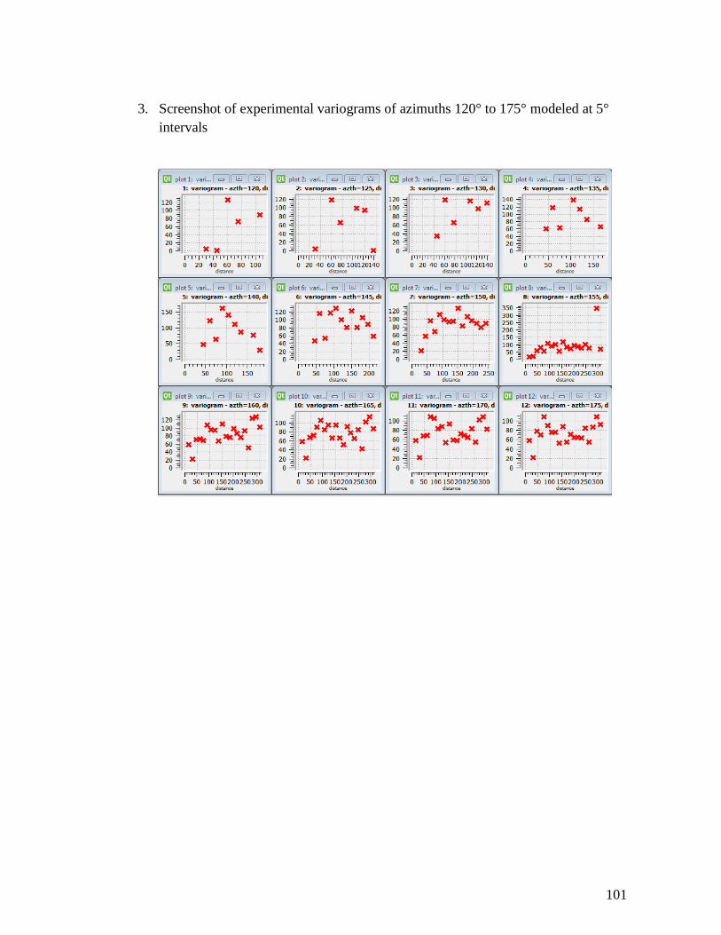
101
3. Screenshot of experimental variograms of azimuths 120° to 175° modeled at 5°
intervals

102
APPENDIX III – INDICATOR VARIOGRAM MODELS FROM SPM3
> 5 TO
SPM3 >26 THRESHOLDS
1.Spherical variogram model at >5 Spm3 cut-off and resepctive map output. Nugget,
sill contribution and range modelled at 0.03, 0.245 and 108.75m respectively
2. Spherical variogram model at >6 Spm3 cut-off. Nugget, sill contribution and range
modelled at 0.03, 0.24 and 101.75m respectively

103
3.Spherical variogram model at >7 Spm3 cut-off and resepctive map output. Nugget,
sill contribution and range modelled at 0.03, 0.25 and 101.75m respectively
4.Spherical variogram model at >8 Spm3 cut-off. Nugget, sill contribution and range
modelled at 0.05, 0.23 and 108.75m respectively

104
5. Spherical variogram model at >9 Spm3 cut-off. Nugget, sill contribution and range
modelled at 0.05, 0.22 and 101 m respectively
6. Spherical variogram model at >10 Spm3 cut-off. Nugget, sill contribution and range
modelled at 0.05, 0.22 and 101 m respectively
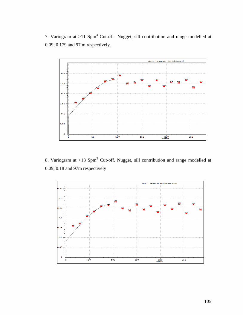
105
7. Variogram at >11 Spm3 Cut-off Nugget, sill contribution and range modelled at
0.09, 0.179 and 97 m respectively.
8. Variogram at >13 Spm3 Cut-off. Nugget, sill contribution and range modelled at
0.09, 0.18 and 97m respectively

106
9. Variogram at >14 Spm3 Cut-off. Nugget, sill contribution and range modelled at
0.1, 0.13 and 78.5 m respectively
10.Variogram at >15Spm3 Cut-off. Nugget, sill contribution and range modelled at
0.1, 0.115and 101 m respectively
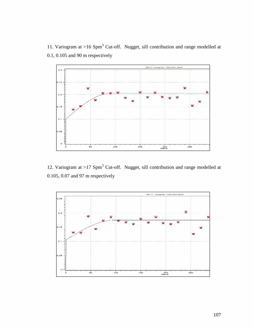
107
11. Variogram at >16 Spm3 Cut-off. Nugget, sill contribution and range modelled at
0.1, 0.105 and 90 m respectively
12. Variogram at >17 Spm3 Cut-off. Nugget, sill contribution and range modelled at
0.105, 0.07 and 97 m respectively

108
13. Variogram at > 18Spm3 Cut-off. Nugget, sill contribution and range modelled at
0.085, 0.08 and 90 m respectively
14. Variogram at >19 Spm3 Cut-off. Nugget, sill contribution and range modelled at
0.08, 0.06 and 71m respectively

109
15. Variogram at >20 Spm3 Cut-off and repective map output. Nugget, sill
contribution and range modelled at 0.08, 0.04 and 75 m respectively
16. Variogram at >21 Spm3 Cut-off. Nugget, sill contribution and range modelled at
0.04, 0.05 and 97.5 m respectively

110
17. Variogram at >22 Spm3 Cut-off. Nugget, sill contribution and range modelled at
0.04, 0.05 and 97.5 m respectively
18. Variogram at >23 Spm3 Cut-off. Nugget, sill contribution and range modelled at
0.028, 0.05 and 97.5 m respectively

111
19. Variogram at >25 Spm3 Cut-off. Nugget, sill contribution and range modelled at
0.04, 0.05 and 97.5 m respectively
20. Variogram at >26 Spm3 Cut-off and respective map output. Nugget, sill
contribution and range modelled at 0.004, 0.04 and 97.5 m respectively

112
21. Variogram at >27 Spm3 Cut-off. Nugget, sill contribution and range modelled at
0.004, 0.04 and 97.5 m respectively

113
APPENDIX IV-PROGRESSIVE STATISTICS DATA
Rea
lisatio
n
No
of P
oin
ts
Blo
ck
s
Estim
ate
d
Mea
n
of
Po
int
Sim
ula
tion
Va
r o
f Poin
t
Sim
ula
tion
s
Po
int
Sim
Std
Dev
Po
int
Sim
ula
tion
s
CO
V
Mea
n
Blk
Sim
ula
tion
s
Va
r B
LK
Sim
ula
tion
s
Std
D
ev
o
f
Blk
Sim
ula
tion
s
BL
K C
OV
Mea
n
Ra
w
Da
ta
Va
r
Ra
w
Da
ta
Std
Dev
Ra
w
Da
ta
CO
V
Ra
w
da
ta
0 205200 2052 10.79 79.597 8.92 1.21 10.21 52.78 7.26 1.41 10.7 79.5 8.9 1.20
1 205200 2052 10.79 79.597 8.92 1.21 10.79 58.03 7.62 1.42 10.7 79.5 8.9 1.20
2 205200 2052 10.89 79.597 8.92 1.22 10.89 54.12 7.36 1.48 10.7 79.5 8.9 1.20
3 205200 2052 10.79 79.597 8.92 1.21 10.79 54.20 7.36 1.47 10.7 79.5 8.9 1.20
4 205200 2052 10.79 79.597 8.92 1.21 10.79 56.36 7.51 1.44 10.7 79.5 8.9 1.20
5 205200 2052 10.79 79.597 8.92 1.21 10.79 57.70 7.60 1.42 10.7 79.5 8.9 1.20
6 205200 2052 10.79 79.597 8.92 1.21 10.79 54.39 7.37 1.46 10.7 79.5 8.9 1.20
7 205200 2052 10.79 79.6694 8.93 1.21 10.79 58.44 7.64 1.41 10.7 79.5 8.9 1.20
8 205200 2052 10.79 79.597 8.92 1.21 10.79 53.95 7.35 1.47 10.7 79.5 8.9 1.20
9 205200 2052 10.79 79.597 8.92 1.21 10.79 54.07 7.35 1.47 10.7 79.5 8.9 1.20
10 205200 2052 10.79 79.597 8.92 1.21 10.79 53.36 7.30 1.48 10.7 79.5 8.9 1.20
11 205200 2052 10.80 80.61 8.98 1.20 10.80 56.99 7.55 1.43 10.7 79.5 8.9 1.20
12 205200 2052 10.79 79.73 8.93 1.21 10.79 56.99 7.55 1.43 10.7 79.5 8.9 1.20
13 205200 2052 10.79 79.597 8.92 1.21 10.79 52.93 7.27 1.48 10.7 79.5 8.9 1.20
14 205200 2052 10.79 79.597 8.92 1.21 10.79 56.09 7.49 1.44 10.7 79.5 8.9 1.20
15 205200 2052 10.79 79.597 8.92 1.21 10.79 55.70 7.46 1.45 10.7 79.5 8.9 1.20
16 205200 2052 10.79 79.597 8.92 1.21 10.79 51.88 7.20 1.50 10.7 79.5 8.9 1.20
17 205200 2052 10.79 79.597 8.92 1.21 10.79 52.87 7.27 1.48 10.7 79.5 8.9 1.20
18 205200 2052 10.79 79.597 8.92 1.21 10.79 55.11 7.42 1.45 10.7 79.5 8.9 1.20
19 205200 2052 10.80 80.57 8.98 1.20 10.80 59.05 7.68 1.41 10.7 79.5 8.9 1.20
20 205200 2052 10.79 79.597 8.92 1.21 10.79 56.01 7.48 1.44 10.7 79.5 8.9 1.20
21 205200 2052 10.79 79.6365 8.92 1.21 10.79 56.04 7.49 1.44 10.7 79.5 8.9 1.20
22 205200 2052 10.79 79.61 8.92 1.21 10.79 55.18 7.43 1.45 10.7 79.5 8.9 1.20
23 205200 2052 10.79 79.597 8.92 1.21 10.79 52.13 7.22 1.49 10.7 79.5 8.9 1.20
24 205200 2052 10.79 79.597 8.92 1.21 10.79 54.73 7.40 1.46 10.7 79.5 8.9 1.20
25 205200 2052 10.79 79.597 8.92 1.21 10.79 51.37 7.17 1.51 10.7 79.5 8.9 1.20
26 205200 2052 10.79 79.597 8.92 1.21 10.79 56.63 7.53 1.43 10.7 79.5 8.9 1.20
27 205200 2052 10.79 79.597 8.92 1.21 10.79 55.17 7.43 1.45 10.7 79.5 8.9 1.20
28 205200 2052 10.79 79.597 8.92 1.21 10.79 56.17 7.49 1.44 10.7 79.5 8.9 1.20
29 205200 2052 10.79 79.597 8.92 1.21 10.79 54.27 7.37 1.46 10.7 79.5 8.9 1.20
30 205200 2052 10.79 79.597 8.92 1.21 10.79 54.39 7.37 1.46 10.7 79.5 8.9 1.20
31 205200 2052 10.79 79.597 8.92 1.21 10.79 54.43 7.38 1.46 10.7 79.5 8.9 1.20
32 205200 2052 10.79 79.9064 8.94 1.21 10.79 55.64 7.46 1.45 10.7 79.5 8.9 1.20
33 205200 2052 10.79 79.597 8.92 1.21 10.79 55.25 7.43 1.45 10.7 79.5 8.9 1.20
34 205200 2052 10.79 79.597 8.92 1.21 10.79 51.69 7.19 1.50 10.7 79.5 8.9 1.20
35 205200 2052 10.79 79.597 8.92 1.21 10.79 53.28 7.30 1.48 10.7 79.5 8.9 1.20

114
10.10
10.20
10.30
10.40
10.50
10.60
10.70
10.80
10.90
11.00
0 10 20 30 40 50
Pro
gre
siv
e M
ean
No of Realisations
Number of realisations Vs Mean
Mean Point
Mean Blk
Rea
lisatio
n
No
of P
oin
ts
Blo
ck
s
Estim
ate
d
Mea
n
of
Po
int
Sim
ula
tion
Va
r o
f Poin
t
Sim
ula
tion
s
Po
int
Sim
Std
Dev
Po
int
Sim
ula
tion
s
CO
V
Mea
n
Blk
Sim
ula
tion
s
Va
r B
LK
Sim
ula
tion
s
Std
D
ev
o
f
Blk
Sim
ula
tion
s
BL
K C
OV
Mea
n
Ra
w
Da
ta
Va
r
Ra
w
Da
ta
Std
Dev
Ra
w
Da
ta
CO
V
Ra
w
da
ta
36 205200 2052 10.79 79.598 8.92 1.21 10.79 54.02 7.35 1.47 10.7 79.5 8.9 1.20
37 205200 2052 10.79 79.597 8.92 1.21 10.79 52.47 7.24 1.49 10.7 79.5 8.9 1.20
38 205200 2052 10.79 79.597 8.92 1.21 10.79 56.08 7.49 1.44 10.7 79.5 8.9 1.20
39 205200 2052 10.79 79.597 8.92 1.21 10.79 54.47 7.38 1.46 10.7 79.5 8.9 1.20
40 205200 2052 10.79 79.597 8.92 1.21 10.79 56.47 7.51 1.44 10.7 79.5 8.9 1.20
41 205200 2052 10.79 79.5986 8.92 1.21 10.79 53.87 7.34 1.47 10.7 79.5 8.9 1.20
42 205200 2052 10.81 81.06 9.00 1.20 10.81 58.81 7.67 1.41 10.7 79.5 8.9 1.20
43 205200 2052 10.79 79.597 8.92 1.21 10.79 57.00 7.55 1.43 10.7 79.5 8.9 1.20
44 205200 2052 10.79 79.597 8.92 1.21 10.79 55.88 7.48 1.44 10.7 79.5 8.9 1.20
45 205200 2052 10.79 79.597 8.92 1.21 10.79 54.75 7.40 1.46 10.7 79.5 8.9 1.20
46 205200 2052 10.79 79.597 8.92 1.21 10.79 54.40 7.38 1.46 10.7 79.5 8.9 1.20
47 205200 2052 10.79 79.597 8.92 1.21 10.79 54.53 7.38 1.46 10.7 79.5 8.9 1.20
48 205200 2052 10.79 79.597 8.92 1.21 10.79 56.10 7.49 1.44 10.7 79.5 8.9 1.20
49 205200 2052 10.79 79.597 8.92 1.21 10.79 54.19 7.36 1.47 10.7 79.5 8.9 1.20
Plot of progressive mean against the number of realisations for block Point and Block
simulations
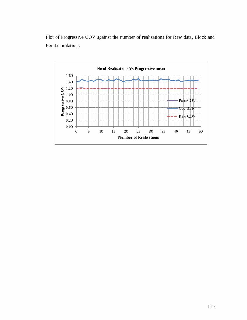
115
0.00
0.20
0.40
0.60
0.80
1.00
1.20
1.40
1.60
0 5 10 15 20 25 30 35 40 45 50
Pro
gre
ssiv
e C
OV
Number of Realisations
No of Realisations Vs Progressive mean
PointCOV
Cov BLK
Raw COV
Plot of Progressive COV against the number of realisations for Raw data, Block and
Point simulations

116
APPENDIX V-SUMMARY OF REALISATION STATISTICS
Rea
lisatio
n
No
Gaussian
Statistics
Back-
transformed
Stats Histograms
Co
rrela
tion
Co
efficient
Co
rrela
tion
coefficien
t
differ
ence
s
Mea
n
Va
rian
ce
Mea
n
Va
rian
ce
Sim
ula
ted
Mea
n/D
rillho
le
Av
era
ge (%
)
Sim
ula
ted
va
rian
ce/Drillh
ole
Va
rian
ce (%)
0 0.17 0.83 10.78 79.5 100.7 103.9 0.88 0.12
1 -0.03 1 10.78 79.5 100.7 103.9 0.89 0.11
2 0.03 0.88 10.79 79.6 100.7 104.1 0.87 0.13
3 -0.03 0.84 10.78 79.5 100.7 103.9 0.79 0.21
4 -0.016 0.97 10.79 79.6 100.7 104.1 0.86 0.14
5 -0.05 0.99 10.79 79.6 100.7 104.1 0.84 0.16
6 0.12 0.89 10.79 79.6 100.7 104.1 0.85 0.15
7 -0.014 1.1 10.79 79.7 100.7 104.2 0.86 0.14
8 0.08 0.86 10.79 79.6 100.7 104.1 0.83 0.17
9 -0.08 0.85 10.79 79.6 100.7 104.1 0.87 0.13
10 0.14 0.85 10.78 79.59 100.7 104.1 0.88 0.12
11 0.12 0.89 10.8 80.61 100.8 105.4 0.84 0.16
12 0.14 0.95 10.79 79.73 100.7 104.2 0.88 0.12
13 0.18 0.85 10.79 79.6 100.7 104.1 0.84 0.16
14 -0.057 0.94 10.79 79.6 100.7 104.1 0.85 0.15
15 -0.13 0.886 10.79 79.6 100.7 104.1 0.85 0.15
16 -0.1285 0.86 10.79 79.6 100.7 104.1 0.88 0.12
17 -0.03 0.84 10.79 79.6 100.7 104.1 0.85 0.15
18 -0.03 0.93 10.79 79.6 100.7 104.1 0.89 0.11
19 0.14 1.03 10.8 80.57 100.8 105.3 0.85 0.15
20 -0.058 0.94 10.79 79.6 100.7 104.1 0.86 0.14
21 -0.02 0.91 10.79 79.64 100.7 104.1 0.82 0.18
22 0.08 0.92 10.79 79.6 100.7 104.1 0.81 0.19
23 -0.03 0.83 10.79 79.6 100.7 104.1 0.86 0.14
24 0.12 0.87 10.79 79.6 100.7 104.1 0.87 0.13
25 0.26 0.8 10.79 79.6 100.7 104.1 0.85 0.15

117
Rea
lisatio
n
No
Gaussian
Statistics
Back-
transformed
Stats Histograms C
orr
elatio
n
Co
efficient
Co
rrela
tion
coefficien
t
differ
ence
s
Mea
n
Va
rian
ce
Mea
n
Va
rian
ce
Sim
ula
ted
Mea
n/D
rillho
le
Av
era
ge (%
)
Sim
ula
ted
va
rian
ce/Drillh
ole
Va
rian
ce (%)
26 0.04 1 10.79 79.6 100.7 104.1 0.85 0.15
27 -0.027 0.92 10.79 79.6 100.7 104.1 0.81 0.19
28 0.04 0.93 10.79 79.6 100.7 104.1 0.84 0.16
29 0.12 0.9 10.79 79.6 100.7 104.1 0.89 0.11
30 -0.17 0.91 10.79 79.6 100.7 104.1 0.85 0.15
31 0.01 0.91 10.79 79.6 100.7 104.1 0.84 0.16
32 0.25 0.94 10.79 79.9 100.7 104.5 0.89 0.11
33 0.013 0.89 10.79 79.9 100.7 104.5 0.88 0.12
34 0.05 0.79 10.79 79.6 100.7 104.1 0.87 0.13
35 0.019 0.86 10.79 79.6 100.7 104.1 0.84 0.16
36 0.21 0.84 10.79 79.6 100.7 104.1 0.84 0.16
37 0 0.81 10.79 79.6 100.7 104.1 0.85 0.15
38 -0.17 0.93 10.79 79.6 100.7 104.1 0.83 0.17
39 0.23 0.91 10.79 79.6 100.7 104.1 0.85 0.15
40 0.59 0.98 10.79 79.6 100.7 104.1 0.88 0.12
41 0.12 0.87 10.79 79.6 100.7 104.1 0.84 0.16
42 0.16 0.99 10.8 81.06 100.8 106.0 0.86 0.14
43 0.03 0.97 10.79 79.6 100.7 104.1 0.82 0.18
44 -0.002 0.95 10.79 79.6 100.7 104.1 0.86 0.14
45 0.002 0.88 10.79 79.6 100.7 104.1 0.83 0.17
46 0.08 0.92 10.79 79.6 100.7 104.1 0.88 0.12
47 0.09 0.88 10.79 79.6 100.7 104.1 0.88 0.12
48 0.03 0.99 10.79 79.6 100.7 104.1 0.83 0.17
49 -0.2 0.97 10.79 79.6 100.7 104.1 0.84 0.16

118
APPPENDIX VI- SELECTED INDIVIDUAL REALISATIONS
Realisation0
Realisation7
Realisation 15 Realisation 17
Realisation 23,
Realisation27
Realisation 31 Realisation 39
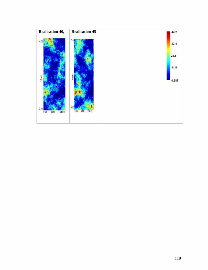
119
Realisation 40,
Realisation 45

120
APPENDIX V11 –15m BENCH INTERVAL AND BLOCK KRIGING MAPS
OUTPUT COMPARED TO SIMULATED MAPS OUTPUT PER BENCH
INTERVAL
ELEVATION BENCH
725 1
710 2
690 3
675 4
660 5
645 6
630 7
615 8
600 9
585 10
570 11
555 12
540 13
525 14
510 15
495 16
480 17
465 18

121
Kriging Map Outputs Simulation Maps Output
1 1
3
3

122
Kriging Map Outputs Simulation Maps Output
5
5
7
7

123
Kriging Map Outputs Simulation Maps Output
9
9
11
11
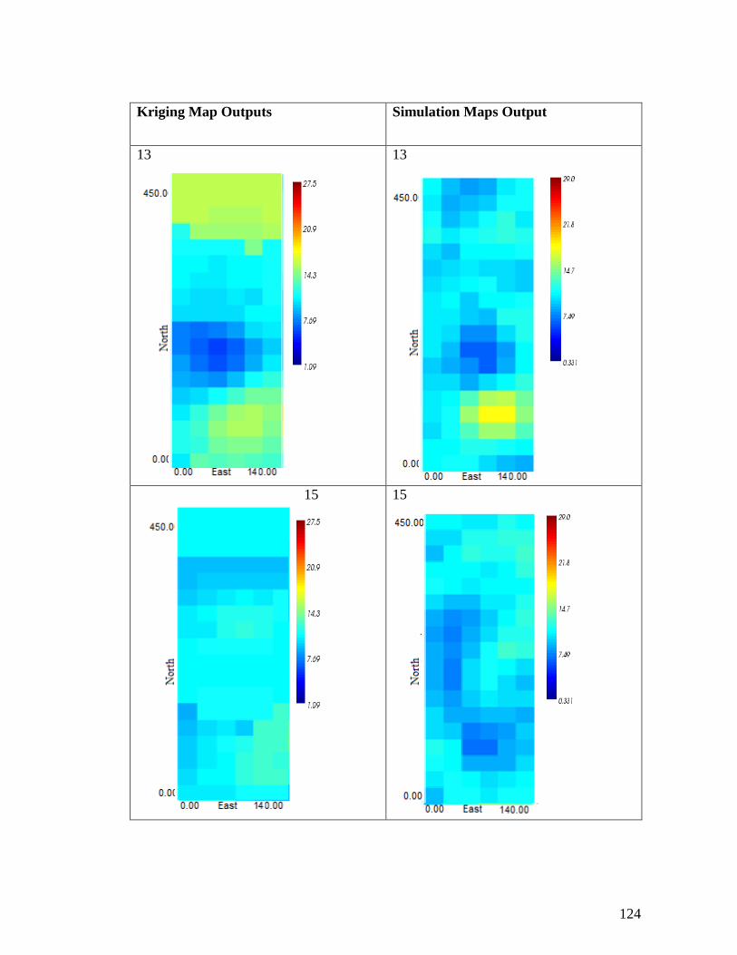
124
Kriging Map Outputs Simulation Maps Output
13
13
15
15

125
Kriging Map Outputs Simulation Maps Output
17
17