GEOSTATISTICAL TEXTURE CLASSIFICATION OF TROPICAL RAINFOREST ININDONESIA

A. WIJAYA∗, P.R. MARPU and R. GLOAGUEN

Remote Sensing Group, Institute for Geology, TU-Bergakademie, B. von-Cottastr. 2, 09599 Freiberg, Germany∗Corresponding author. Tel: +49-(0)3731-444167, Email address: Arief.Wijaya@student.tu-freiberg.de

http://www.geo.tu-freiberg.de/fernerkundung/

KEY WORDS: spectral classification, tropical rainforests, semivariogram, texturelayers, geostatistics

ABSTRACT:

Traditional spectral classification of remote sensing data applied on per pixel basis ignores the potentially useful spatial informationbetween the values of proximate pixels. Although spatial information extraction has been greatly explored, there have been limitedattempts to enhance classification by combining spectral and spatial information. This improvement would arise from the hypothesisthat a pixel is not independent of its neighbors and, furthermore, thatits dependence can be quantified and incorporated into theclassifier.This study aims to explore the potential of utilizing texture spatial variability usinggeostatistics and Grey Level Co-occurrence Matrix(GLCM) texture measures. Different texture layers derived from geostatistics method, namely fractal dimension, semivariogram, mado-gram, rodogram, pseudo-cross variogram and pseudo-cross madogram, were incorporated for the land cover classification of tropicalrainforests in East Kalimantan, Indonesia. Texture layers of grey level co-occurrence matrix (GLCM) channels, i.e. variance, contrast,dissimilarity, and homogeinity, were also used for the classification. Two classification methods, using Support Vector Machine andMinimum distance were applied for image classification.Landsat 7 ETM images combined with textural information is used for land cover classification of tropical rainforest area. Band 5 ofLandsat data was used to compute texture layers using the GLCM and geostatistics methods. This band was chosen because it has thehighest variance of training data compared to other spectral bands.The results were compared to find out how the extra information given bythe texture enhances the classification. According to theaccuracy assessment using error matrix, combinations of image and texture data performed better with81% of accuracy compared tothose of image data only with76% of accuracy.

1 INTRODUCTION

Mapping of forest cover is an ultimate way to assess forest coverchanges and to study forest resource within a period of time. Onthe other hand, forest encroachment is hardly stopped recentlydue to excessive human exploitation on forest resources. The for-est encroachment is even worse in the tropical forest, which ismostly located in developing countries, where forest timber is avery valuable resource. The needs for the updated and accuratemapping of forest cover is an urgent requirement in order to mon-itor and to properly manage the forest area.

Remote sensing is a promising tool for mapping and classifica-tion of forest cover. A huge area can be monitored efficientlyat a very high speed and relatively low cost using remote sens-ing data. Interpretation of satellite image data mostly applies aper pixel classification rather than the correlation with neighbor-ing pixels. Geostatistics is a method, that may be used for imageclassification, as we can consider spatial variability among neigh-boring pixels (Jakomulska and Clarke, 2001). Geostatistics andthe theory of regionalized variables have already been introducedto remote sensing (Woodcock et al., 1988).

This work attempts to carry out image classification by incor-porating texture information. Texture represents the variationof grey values in an image, which provides important informa-tion about the structural arrangements of the image objects andtheir relationship to the environment (Chica-Olmo and Abarca-Hernandez, 2000). The work aims to explore the potential ofpixel classification by measuring texture spatial variability usinggeostatistics, fractal dimension, and conventional GLCM meth-ods. This is encouraged by several factors, like:(1) texture fea-tures can improve image classification results, as we include extra

information; (2) image classification on forest area, where visu-ally there are no apparent distinct objects to be discriminated (e.g.shape, boundary) can take into benefit the use of texture variationto carry out the classification; and(3) texture features of landcover classes in forest area, as depicted on Figure 1 are quite dif-ferent visually even if the spectral values are similar; therefore theuse of texture features may improve the classification accuracy.

2 STUDY AREA

The study focuses on a forest area located in Labanan concessionforest, Berau municipality, East Kalimantan Province, Indonesiaas described on Figure 2. This area geographically lies between1◦ 45’ to 2◦ 10’ N, and 116◦ 55 and 117◦ 20’ E.

The forest area belongs to a state owned timber concession-holdercompany where timber harvesting activity is carried out, and thearea mainly situated on inland of coastal swamps and formed byundulating to rolling plains with isolated masses of high hills andmountains. The variation in topography is a consequence of fold-ing and uplift of rocks, resulting from tension in the earth crust.The landscape of Labanan is classified into flat land, sloping land,steep land, and complex landforms, while the forest type is oftencalled as lowland mixed dipterocarp forest.

3 DATA AND METHOD

3.1 Data

Landsat 7 ETM of path 117 and row 59 acquired on May 31, 2003with 30 m resolution was used in this study. The data were ge-ometrically corrected using WGS 84 datum and UTM projection

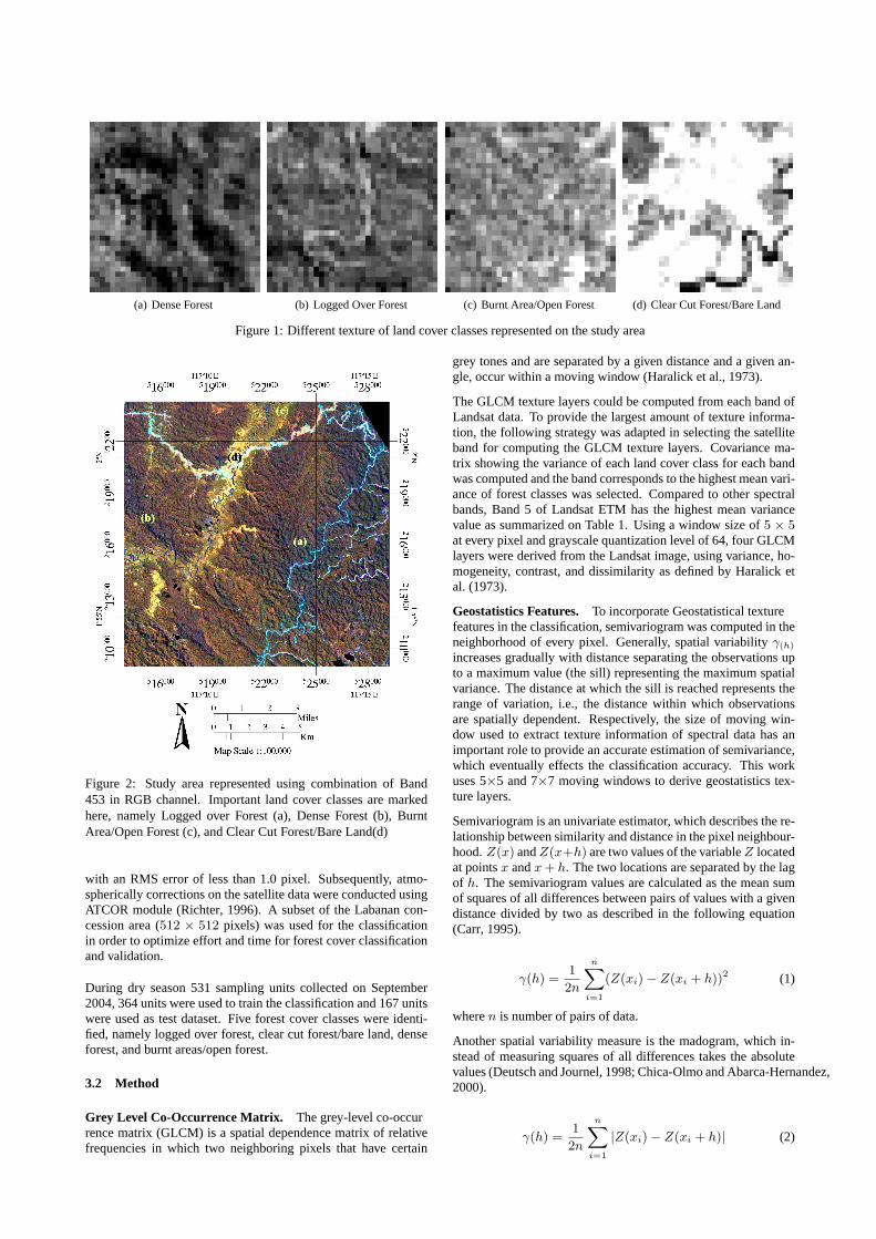
(a) Dense Forest (b) Logged Over Forest (c) Burnt Area/Open Forest (d) Clear Cut Forest/Bare Land

Figure 1: Different texture of land cover classes represented on the study area

Figure 2: Study area represented using combination of Band453 in RGB channel. Important land cover classes are markedhere, namely Logged over Forest (a), Dense Forest (b), BurntArea/Open Forest (c), and Clear Cut Forest/Bare Land(d)

with an RMS error of less than 1.0 pixel. Subsequently, atmo-spherically corrections on the satellite data were conducted usingATCOR module (Richter, 1996). A subset of the Labanan con-cession area (512 × 512 pixels) was used for the classificationin order to optimize effort and time for forest cover classificationand validation.

During dry season 531 sampling units collected on September2004, 364 units were used to train the classification and 167 unitswere used as test dataset. Five forest cover classes were identi-fied, namely logged over forest, clear cut forest/bare land, denseforest, and burnt areas/open forest.

3.2 Method

Grey Level Co-Occurrence Matrix. The grey-level co-occurrence matrix (GLCM) is a spatial dependence matrix of relativefrequencies in which two neighboring pixels that have certain

grey tones and are separated by a given distance and a given an-gle, occur within a moving window (Haralick et al., 1973).

The GLCM texture layers could be computed from each band ofLandsat data. To provide the largest amount of texture informa-tion, the following strategy was adapted in selecting the satelliteband for computing the GLCM texture layers. Covariance ma-trix showing the variance of each land cover class for each bandwas computed and the band corresponds to the highest mean vari-ance of forest classes was selected. Compared to other spectralbands, Band 5 of Landsat ETM has the highest mean variancevalue as summarized on Table 1. Using a window size of5 × 5at every pixel and grayscale quantization level of 64, four GLCMlayers were derived from the Landsat image, using variance, ho-mogeneity, contrast, and dissimilarity as defined by Haralick etal. (1973).

Geostatistics Features. To incorporate Geostatistical texturefeatures in the classification, semivariogram was computed in theneighborhood of every pixel. Generally, spatial variabilityγ(h)

increases gradually with distance separating the observations upto a maximum value (the sill) representing the maximum spatialvariance. The distance at which the sill is reached represents therange of variation, i.e., the distance within which observationsare spatially dependent. Respectively, the size of moving win-dow used to extract texture information of spectral data has animportant role to provide an accurate estimation of semivariance,which eventually effects the classification accuracy. This workuses 5×5 and 7×7 moving windows to derive geostatistics tex-ture layers.

Semivariogram is an univariate estimator, which describes the re-lationship between similarity and distance in the pixel neighbour-hood.Z(x) andZ(x+h) are two values of the variableZ locatedat pointsx andx + h. The two locations are separated by the lagof h. The semivariogram values are calculated as the mean sumof squares of all differences between pairs of values with a givendistance divided by two as described in the following equation(Carr, 1995).

γ(h) =1

2n

n∑

i=1

(Z(xi) − Z(xi + h))2 (1)

wheren is number of pairs of data.

Another spatial variability measure is the madogram, which in-stead of measuring squares of all differences takes the absolutevalues (Deutsch and Journel, 1998; Chica-Olmo and Abarca-Hernandez,2000).

γ(h) =1

2n

n∑

i=1

|Z(xi) − Z(xi + h)| (2)

Land Cover Class Band 1 Band 2 Band 3 Band 4 Band 5 Band 6 Band 7

Logged Over Forest 3.49 3.03 8.46 23.56 50.98 0.70 15.46Burnt Areas/Open Forest 2.59 1.76 2.59 24.19 18.46 0.46 5.04Road Network 65.68 165.39 332.63 74.12 386.45 1.91 294.98Clear Cut Forest/Bare Land 2.70 5.20 2.90 33.52 32.49 0.83 8.70Dense Forest 2.92 1.56 1.49 1.82 11.08 0.49 4.73Hill Shadow 2.62 2.78 2.58 40.28 30.32 0.57 6.63

Mean Variance of total classes 13.33 29.95 58.44 32.91 88.30 0.83 55.92

Table 1: Variance matrix of forest cover classes training data

By calculating square root of absolute differences, we can derivea spatial variability measure called rodogram as shown in the fol-lowing formula (Lloyd et al., 2004).

γ(h) =1

2n

n∑

i=1

|Z(xi) − Z(xi + h)|1

2 (3)

Alternatively, three multivariate estimators quantify the joint spa-tial variability (cross correlation) between two bands, namely pseudocross variogram, and pseudo cross madogram were also com-puted. The pseudo-cross variogram represents the semivarianceof the cross increments, and calculated as follows.

γ(h) =1

2n

n∑

i=1

(Y (xi) − Z(xi + h))2 (4)

The pseudo-cross madogram is similar of the pseudo-cross vari-ogram, but again, instead of squaring the differences, the absolutevalues of the differences area taken, which leads to a more gener-ous behavior toward outliers (Buddenbaum et al., 2005).

γ(h) =1

2n

n∑

i=1

|Y (xi) − Z(xi + h)| (5)

Using Band 5 of Satellite data, the spatial variability measureswere computed and median values of semivariance at each com-puted lag distance were taken, resulted in the full texture layersfor each calculated spatial variability measure. These texture lay-ers were then put as additional input for the classification.

Fractal Dimension. Fractal is defined as an object which areself-similar and show scale invariance (Carr, 1995). Fractal dis-tribution requires that the number of objects larger than a speci-fied size has a power law dependence on the size. Every fractal ischaracterized by a fractal dimension (Carr, 1995).

Given the semivariogram of any spatial distribution, fractal di-mension(D) is commonly estimated using the relationship be-tween the fractal dimension of a series and the slope of the corre-sponding log-log semivariogram(m) plot (Burrough, 1983; Carr,1995).

D = 2 −m

2(6)

4 RESULTS & DISCUSSION

4.1 Results

Before Geostatistics texture layers were derived, we observedwhether there is textural variation among different classes. Using

training data, semivariogram of land cover classes on the studyarea was sequentially computed for lag distance (range) of 30pixels, as presented on Figure 3.

γ

Distance

Variogram plot

.0 5.0 10.0 15.0 20.0 25.0

.0

10.0

20.0

30.0

40.0

50.0

60.0

70.0

80.0

Figure 3: Variogram plot of training data shows the spatial vari-ability of land cover classes on the study area, i.e. logged overforest (red), burnt areas/open forest (blue), clear cut forest/bareland (yellow), dense forest (green), hill shadow (purple)

As shown in Figure 3, semivariance computed for every lag dis-tance may provide useful information for data classification asthose values of each forest class revealed spatial correlation forlag distance of less than 10 pixels. However, there is an excep-tional case for dense forest class, which shows spatial variabil-ity on larger lag. This may be a problem for computing semi-variance for this particular class as the calculation of per pixelsemivariance on large lag distance is computationally expensive.Compromising with other forest classes, texture layers were com-puted using 5×5 and 7×7 moving windows. Using different spa-tial variability measures explained before, semivariance valuesfor each pixel were calculated and median of these values wasused, resulting in texture information of the study area. The re-sults of Geostatistics texture layers are described on Figure 4.

Classification of satellite image was done using following datacombinations:(1) ETM data;(2) ETM data and GLCM texture,and; (3) ETM data and Geostatistics texture. Two classificationmethods, using minimum distance algorithm and Support Vec-tor Machine (SVM) method were applied for the purpose of thestudy.

The SVM method is originally a binary classifier, that is basedon statistical learning theory (Vapnik, 1999). Multi-class imageclassification using the SVM method is conducted by combin-ing several binary classification to segmenting data with the sup-port of optimum hyperplane. The optimum performance of thismethod mainly affected by a proper set up of some parametersinvolved in the algorithm. This study, however, was not tryingto optimize the SVM classification, therefore those parameterswere arbitrarily determined. For the classification, Radial Basis

1.3

1.4

1.5

1.6

1.7

1.8

1.9

2

2.1

(a) Fractal Dimension

2

4

6

8

10

12

14

(b) Madogram

1

1.5

2

2.5

3

3.5

4

(c) Rodogram

200

400

600

800

1000

1200

1400

1600

1800

2000

(d) Semivariogram

5

10

15

20

25

(e) Pseudo-Cross Madogram

200

400

600

800

1000

1200

1400

(f) Pseudo-Cross Semivariogram

Figure 4: Different texture layers derived from spatial variability measures of Geostatistics Method

Function kernel was used,γ in kernel and classification proba-bility threshold were respectively,0.143 and0.0, while penaltyparameter was100.

The motivation of using those two methods for classifying spatialand texture data was in order to study the performance of texturedata given two completely different algorithms in the classifica-tion. The classification results are summarized on Table 2.

Applying the SVM and Minimum Distance in the classification,the results showed that74% and76% of accuracies were achievedwhen Band 3,4,5 of Landsat image and multipectral Landsat data(i.e. Band 1-5,7) were used in the classification, respectively.Furthermore, multispectral bands of Landsat data were used toperform classification using texture data.

The GLCM texture layers have slightly improved the classifica-tion accuracies, when variance, contrast, and dissimilarity wereused in the classification. The GLCM texture classification per-formed by the SVM resulted in81% of accuracy when combina-tion of ETM data and all the GLCM texture layers were applied.

Geostatistics texture layers, on the other hand, performed quitesatisfactorily, resulting more than80% of accuracies when frac-tal dimension, madogram, rodogram and combination of thosetexture layers were used in the classification. The classificationresulted in81.44% of accuracy and kappa of0.78 when imagedata, fractal dimension, madogram and rodogram were classifiedby the SVM method, the results were depicted on Figure 5.

Figure 5: The final classification result image

Indeed, the SVM performed better than Minimum Distance, whentexture data was used, it has already been proven that the SVMperformed well dealing with large spectral data resolution, suchas hyperspectral, as reported by several recent studies (Gualtieriand Cromp, 1999; Pal and Mather, 2004, 2005).

4.2 Discussion

Geostatistics texture layers performed quite well in the classifica-tion. However, semivariogram and pseudo-cross semivariogramtexture layers were not giving satisfactory classification resultswhen those layers were classified by Minimum Distance method.This is due the nature of semivariogram and pseudo-cross semi-variogram, which calculate the mean square of semivariance forall observed lag distance, either using monovariate or multivariateestimators. This, eventually may reduce the classification accu-racy because of the presence of data outliers.

Combined with madogram and rodogram, the classification re-sulted in higher accuracies with the SVM and Minimum Distancemethod methods. This is obvious as madogram, calculating thesum of absolute value of semivariance for all observed lag dis-tance, and rodogram, computing the sum of square root of thosesemivariance, have ’softer’ effect to the presence of outliers com-pared to those of semivariogram.

This study observed that by changing the size of moving win-dow from5 × 5 into 7 × 7 has slightly improved the classifica-tion accuracy. This is because the scale of land cover texture issimilar with the the7 × 7 window size; therefore, this windowsize provides more texture information than the other. However,computation of texture layer using larger size of moving windowis absolutely not efficient in terms of time, thus to initially findthe optimum size of moving window may be an alternative to re-duce efforts and time for the computation of geostatistics texturelayers. Selection of proper size of moving window will providebetter texture information resulted from spectral image data.

In general, additional texture layers for image classification, ei-ther derived from the GLCM or Geostatistics, have effectivelyimproved the classification accuracy. Although, this study foundthat by applying different GLCM texture layers as well as Geo-statistics layers in a single classification process considerably im-proved classification accuracy, one should be very careful to ap-ply the same method for different types of data. The selection ofclassification algorithm depends on the data distribution.

5 CONCLUSIONS AND FUTURE WORK

This study found that texture layers derived from the GLCM andGeostatistics methods have improved classification of spatial dataof Landsat image. Texture layers are computed using the movingwindow method. Selection of the moving window size is veryimportant since extraction of texture information from spectraldata is more useful when texture characteristics corresponds tothe observed land cover classes are already known.

Support Vector Machine as well as Minimum Distance algorithmwere performed well in the classification elaborating texture dataas additional input of Landsat ETM data. Moreover, the SVMresulted on average higher accuracies compared to those of Min-imum Distance Method.

The authors observed that for future work, it is also possible tocompute Geostatistics texture layer with adjustable moving win-dow size, depending on the size of texture polygon for certainland cover class being observed. This may be an alternative toextract better texture information from spectral data.

ACKNOWLEDGEMENTS

The Landsat ETM and ground truth data were collected whenthe first author joined to the MONCER Project during his master

Min. Distance SVMOAA (%) Kappa OAA (%) Kappa

ETM DataETM 6 Bands 76% 0.71 76% 0.71ETM Band 3,4,5 74% 0.69 74% 0.71

ETM 6 Bands, Geo-Texture Windows 5×5ETM 6 Bands, Fractal 76% 0.71 81% 0.77ETM 6 Bands, Madogram 77% 0.72 78% 0.74ETM 6 Bands, Rodogram 76% 0.71 80% 0.76ETM 6 Bands, Semivariogram 57% 0.48 77% 0.72ETM 6 Bands, Pseudo-Cross Semivariogram 47% 0.36 77% 0.72ETM 6 Bands, Pseudo-Cross Madogram 76% 0.71 75% 0.71ETM 6 Bands, Fractal, Madogram, Rodogram 77% 0.72 81% 0.77

ETM 6 Bands, Geo-Texture Windows 7×7ETM 6 Bands, Fractal 76% 0.71 79% 0.75ETM 6 Bands, Madogram 78% 0.73 80% 0.76ETM 6 Bands, Rodogram 76% 0.71 81% 0.77ETM 6 Bands, Semivariogram 50% 0.39 77% 0.73ETM 6 Bands, Pseudo-Cross Semivariogram 47% 0.37 76% 0.71ETM 6 Bands, Pseudo-Cross Madogram 76% 0.71 76% 0.71ETM 6 Bands, Fractal, Madogram, Rodogram 78% 0.73 81% 0.78

ETM 6 Bands, GLCMETM 6 Bands, Variance 77% 0.72 77% 0.72ETM 6 Bands, Contrast 77% 0.72 75% 0.70ETM 6 Bands, Dissimilarity 72% 0.67 77% 0.73ETM 6 Bands, Homogeinity 62% 0.54 77% 0.72ETM 6 Bands, Variance, Contrast, Dissimilarity, Homogeinity 63% 0.55 81% 0.77

Table 2: Overall Accuracy Assessment (OAA) of the Classification

studying in the International Institute for Geo-Information Sci-ence and Earth Observation the Netherlands. Therefore, the firstauthor would like to thanks to Dr. Ali Sharifi and Dr. YousifAli Hussein, who make possible of data collection used for thepurpose of this study.

References

Buddenbaum, H., Schlerf, M. and Hill, J., 2005. Classificationof coniferous tree species and age classes using hyperspectraldata and geostatistical methods. International Journal of Re-mote Sensing 26(24), pp. 5453–5465.

Burrough, P. A., 1983. Multiscale sources of spatial variation insoil. ii. a non- brownian fractal model and its application in soilsurvey. Journal of Soil Science 34(3), pp. 599–620.

Carr, J., 1995. Numerical Analysis for the Geological Sciences.Prentice - Hall, Inc, NJ.

Chica-Olmo, M. and Abarca-Hernandez, F., 2000. Computinggeostatistical image texture for remotely sensed data classifi-cation. Computers and Geosciences 26(4), pp. 373–383.

Deutsch, C. and Journel, A., 1998. GSLIB: geostatistical soft-ware library and user’s guide. Second edition. GSLIB: geo-statistical software library and user’s guide. Second edition,Oxford University Press.

Gualtieri, J. and Cromp, R., 1999. Support vector machines forhyperspectral remote sensing classification. Proceedings ofSPIE - The International Society for Optical Engineering 3584,pp. 221–232.

Haralick, R., Shanmugam, K. and Dinstein, I., 1973. Texturalfeatures for image classification. IEEE Transactions on Sys-tems, Man and Cybernetics smc 3(6), pp. 610–621.

Jakomulska, A. and Clarke, K., 2001. Variogram-derived mea-sures of textural image classification. In: P. Monesties (ed.),geoENV III - Geostatistics for Environment Applications,Kluwer Academic Publisher, pp. 345–355.

Lloyd, C., Berberoglu, S., Curran, P. and Atkinson, P., 2004. Acomparison of texture measures for the per-field classificationof mediterranean land cover. International Journal of RemoteSensing 25(19), pp. 3943–3965.

Pal, M. and Mather, P., 2004. Assessment of the effectiveness ofsupport vector machines for hyperspectral data. Future Gener-ation Computer Systems 20(7), pp. 1215–1225.

Pal, M. and Mather, P., 2005. Support vector machines for clas-sification in remote sensing. International Journal of RemoteSensing 26(5), pp. 1007–1011.

Richter, R., 1996. Atmospheric correction of satellite data withhaze removal including a haze/clear transition region. Com-puters and Geosciences 22(6), pp. 675–681.

Vapnik, V., 1999. An overview of statistical learning theory. IEEETransactions on Neural Networks 10(5), pp. 988–999.

Woodcock, C. E., Strahler, A. H. and Jupp, D. L. B., 1988. Theuse of variograms in remote sensing: Ii. real digital images.Remote Sensing of Environment 25(3), pp. 349–379.