geostatistical tools for modeling and interpreting...
TRANSCRIPT
Ecological .\lonographs 62(2). 1992. pp. 277-314 6 1992 by the Ecological Society of America
GEOSTATISTICAL TOOLS FOR MODELING AND INTERPRETING ECOLOGICAL SPATIAL
DEPENDENCE1
RICHARD E. ROSSI Department of Applied Earth Sciences, Stanford C’niversity, Stanford, California 94305-2225 C’SA
DAVID J. MULLA Department of Agronomy and Soils, Washington State C’niversity, Pullman, Washington 99164-6420 USA
ANDR~. G. JOURNEL Department of Applied Earth Sciences, Stanford University, Stanford, California 94305-2225 USA
ELDON H. FRANZ Program in Environmental Science and Regional Planning, Washington State University,
Pullman, Washington 99164-4430 C’SA
Abstract. Geostatistics brings to ecology novel tools for the interpretation of spatial patterns of organisms, of the numerous environmental components with which they in- teract, and of the joint spatial dependence between organisms and their environment. The purpose of this paper is to use data from the ecological literature as well as from original research to provide a comprehensive and easily understood analysis ofgeostatistics’ manner of modeling and methods. The traditional geostatistical tool, the variogram, a tool that is beginning to be used in ecology, is shown to provide an incomplete and misleading summary of spatial pattern when local means and variances change. Use of the non-ergodic covariance and correlogram provides a more effective description of lag-to-lag spatial dependence because the changing local means and variances are accounted for. Indicator transforma- tions capture the spatial patterns of nominal ecological variables like gene frequencies and the presence/absence of an organism and of subgroups of a population like large or small individuals. Robust variogram measures are shown to be useful in data sets that contain many data outliers. Appropriate removal of outliers reveals latent spatial dependence and patterns. Cross-variograms, cross-covariances, and cross-correlograms define the joint spa- tial dependence between co-occurring organisms. The results of all of these analyses bring new insights into the spatial relations of organisms in their environment.
Key words: Balanus; Diabrotica; Dyschirius; geostatistical modeling theory and methods: h-scat- tergram: indicator variogram: Mus; non-ergodic correlogram and cross-correlogram: non-ergodic co- variance and cross-covariance; Pterostichus; spatial dependence of organisms in environment; spatial outlier: spatial pattern: variogram and cross-variogram.
INTRODUCTION What is geostatistics and why use it?
Statistical procedures are often used to organize and summarize data so that meaningful inferences can be made about phenomena ofinterest. Commonly in ecol- ogy the foundation of such an inference is a statistical test like a t , F, and x2 test or a procedure like an analysis of variance (ANOVA). These tools are convenient and easy to implement, but they generally assume that any one datum is independent of all other data and that the data are distributed identically. Are these assump- tions tenable for most ecological investigations? We submit that assuming spatial dependence is more prac- tical and realistic, since what we identify as ecological phenomena involves a recognition of correlation.
’ Manuscript received 10 September 1990; revised 25 May 1991; accepted 28 May 1991.
Spatial and temporal dependence or continuity should be readily apparent to the ecologist: vegetation species and densities are generally different on north-facing vs. south-facing slopes; grasshoppers (Orthoptera) are more dense during hot, dry periods; and in greenhouse ex- periments plants are routinely rotated to eliminate microclimatic and microenvironmental (space-time) effects. Ecological analysis normally includes investi- gations of the dispersion and patterns in association between different species at different places and at dif- ferent times (Pielou 1977)-patterns that reflect spatial dependence, not independence. Indeed, the very defi- nitions of ecology, like “the study of the natural en- vironment, particularly the interrelationships between organisms and thir surroundings” (Ricklefs 1973) and “the scientific study of the relationships between or-
ganisms and their environments” (McNaughton and Wolf 1973), or of key concepts, such as levels of or-
278 RICHARD E. ROSS1 ET AL. Ecological Monographs Vol. 62. No. 2
j i,
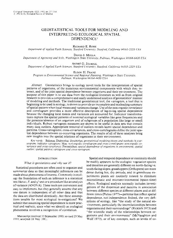
FIG. 1. Perspective plot of Hengeveld’s (1979) summer collection of the carabid Dyschirius globosus on a reclaimed polder. Separation distance between intersection points on the sampling grid is 40 m.
ganization (Odum 1975), presuppose spatial and tem- poral dependence.
Spatial dependence is particularly important in an analysis of spatially varying organism distributions and environmental variables, yet many traditional statis- tical measures tend to ignore it. Consider Hengeveld’s (1979) report of the spatial distribution of a carabid beetle, Dyschirius globosus, on an 800 x 400 m re- claimed Netherland polder. Five pitfall traps were ar- ranged in a hexagon and centered at each node of a 2 1 x 12 sampling grid spaced 40 m apart, and the num- bers of D. globosus caught during the months April- August were reported. A perspective plot (Fig. 1) of the data reveals a marked concentration of the organism around the center of the sampling space. In addition, two areas near the center of this concentration display particularly large values. Overall, the value at any one location is similar to the values at neighboring loca- tions.
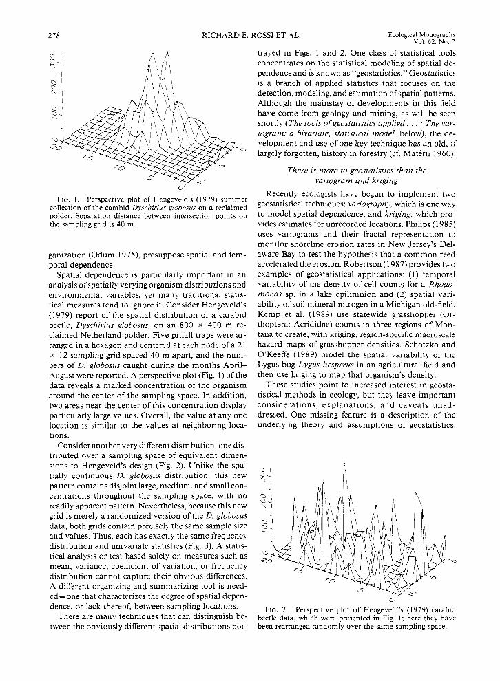
Consider another very different distribution, one dis- tributed over a sampling space of equivalent dimen- sions to Hengeveld’s design (Fig. 2). Unlike the spa- tially continuous D. globosus distribution, this new pattern contains disjoint large, medium, and small con- centrations throughout the sampling space, with no readily apparent pattern. Nevertheless, because this new grid is merely a randomized version of the D. globosus data, both grids contain precisely the same sample size and values. Thus, each has exactly the same frequency distribution and univariate statistics (Fig. 3). A statis- tical analysis or test based solely on measures such as mean, variance, coefficient of variation, or frequency distribution cannot capture their obvious differences. A different organizing and summarizing tool is need- ed- one that characterizes the degree of spatial depen- dence, or lack thereof, between sampling locations.
There are many techniques that can distinguish be- tween the obviously different spatial distributions por-
trayed in Figs. 1 and 2. One class of statistical tools concentrates on the statistical modeling of spatial de- pendence and is known as “geostatistics.” Geostatistics is a branch of applied statistics that focuses on the detection, modeling, and estimation of spatial patterns. Although the mainstay of developments in this field have come from geology and mining, as will be seen shortly (The tools of geostatistics applied. . . : The var- iogram: a bivariate, statistical model, below), the de- velopment and use of one key technique has an old, if largely forgotten, history in forestry (cf. MatCrn 1960).
There is more to geostatistics than the variogram and kriging
Recently ecologists have begun to implement two geostatistical techniques: variography, which is one way to model spatial dependence, and kriging, which pro- vides estimates for unrecorded locations. Philips (1 985) uses variograms and their fractal representation to monitor shoreline erosion rates in New Jersey’s Del- aware Bay to test the hypothesis that a common reed accelerated the erosion. Robertson (1 987) provides two examples of geostatistical applications: ( 1) temporal variability of the density of cell counts for a Rhodo- monas sp. in a lake epilimnion and (2) spatial vari- ability of soil mineral nitrogen in a Michigan old-field. Kemp et al. (1989) use statewide grasshopper (Or- thoptera: Acrididae) counts in three regions of Mon- tana to create, with kriging, region-specific macroscale hazard maps of grasshopper densities. Schotzko and O’Keeffe (1 989) model the spatial variability of the Lygus bug Lygus hesperus in an agricultural field and then use kriging to map that organism’s density.
These studies point to increased interest in geosta- tistical methods in ecology, but they leave important considerations, explanations, and caveats unad- dressed. One missing feature is a description of the underlying theory and assumptions of geostatistics.
FIG. 2. Perspective plot of Hengeveld’s (1979) carabid beetle data, which were presented in Fig. 1; here they have been rearranged randomly over the same sampling space.
June 1992 GEOSTATISTICAL TOOLS FOR ECOLOGY
0
279
These foundations must be appreciated in order that the transfer of the techniques be accomplished effec- tively and correctly. Moreover, the mainstay of geosta- tistical literature can present an often-daunting array of jargon and mathematical and statistical formulas. Our goal is to present a primarily intuitive appreciation of these foundations-one that contains a minimum of mathematical and statistical nomenclature, but one that is rich in ecological examples and yet theoretically rigorous.
More importantly, ecology stands to benefit greatly by a presentation of modeling and estimation tech- niques not utilized in the aforementioned papers. As we show below, unusually large and small data (i.e., outliers) can greatly affect the interpretation of spatial dependence when using the variogram. It is critical, therefore, to be aware of methods for their identifica- tion and to have an understanding of the circumstances in which their removal is valid. Additionally, we pro- vide examples of a type of variogram, known as an “indicator variogram,” that can be used to model the spatial dependence between nominal ecological vari- ables such as gene frequencies. We also show how in- dicator variograms can be used to model the spatial dependence of a particular size class of the organism’s total sample set. This provides a potent new dimension to the traditional variogram because it permits iden- tification of the spatial patterns of ecologically mean- ingful subgroups within a population, like the youngest or smallest individuals vs. the oldest or largest ones.
Other very powerful modeling tools for ecological analysis, ones absent from the above-mentioned pa- pers, model the joint spatial dependence between two co-occurring species or between an organism and a known or suspected influential component of its en- vironment. These techniques strike at the heart ofwhat is ecology.
Finally, and most importantly, using ecological ex- amples we demonstrate that the variogram modeling tool used in the above papers may actually provide an incomplete image of spatial pattern. This is because the variogram is affected strongly by small-scale or local mean and variance differences. Alternative spatial modeling tools are described and illustrated, ones that are more resistant to small-scale data effects. These alternative tools not only uncover spatial dependence more accurately, they can also uncover spatial patterns undetected by the variogram.
We use data from the botanical and zoological lit- erature to describe and illustrate new geostatistical methods. Using already-published data is helpful be- cause a comparison between the findings and the results of geostatistical and conventional analyses can hasten comprehension of new terms and analytic procedures and improve interpretations.
In this paper we describe the underlying rationale and procedures of geostatistics, develop its analytical tools, and delve into some allied techniques that are
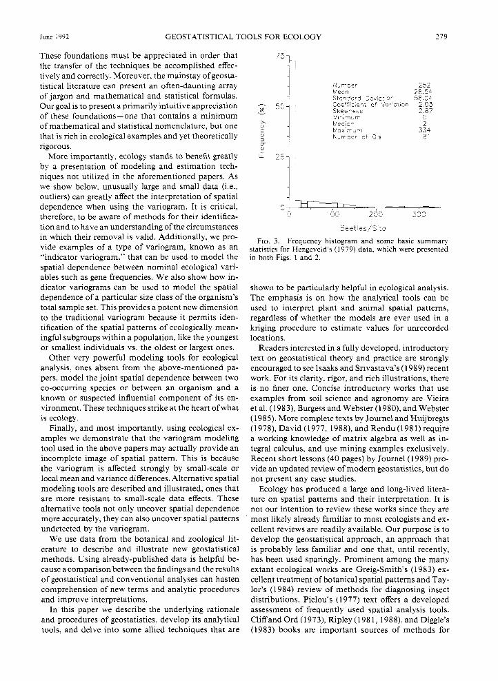
\ U T l 3 € ’ Mean S t a i d a f d Deviar ion Coeff ic ieTt of Variation Skew r e s s Uin,mum M e d i a l M a x i m u m humbe. of 0 ’ s
252 28.54 58.04 2.03 2,87 0 2 334
a1
shown to be particularly helpful in ecological analysis. The emphasis is on how the analytical tools can be used to interpret plant and animal spatial patterns, regardless of whether the models are ever used in a kriging procedure to estimate values for unrecorded locations.
Readers interested in a fully developed, introductory text on geostatistical theory and practice are strongly encouraged to see Isaaks and Srivastava’s ( 1 989) recent work. For its clarity, rigor, and rich illustrations, there is no finer one. Concise introductory works that use examples from soil science and agronomy are Vieira et al. (1 983), Burgess and Webster ( 1 980), and Webster (1985). More complete texts by Journel and Huijbregts (1978), David (1977, 1988), and Rendu(l981) require a working knowledge of matrix algebra as well as in- tegral calculus, and use mining examples exclusively. Recent short lessons (40 pages) by Journel(l989) pro- vide an updated review of modem geostatistics, but do not present any case studies.
Ecology has produced a large and long-lived litera- ture on spatial patterns and their interpretation. It is not our intention to review these works since they are most likely already familiar to most ecologists and ex- cellent reviews are readily available. Our purpose is to develop the geostatistical approach, an approach that is probably less familiar and one that, until recently, has been used sparingly. Prominent among the many extant ecological works are Greig-Smith’s (1983) ex- cellent treatment of botanical spatial patterns and Tay- lor’s (1984) review of methods for diagnosing insect distributions. Pielou’s (1 977) text offers a developed assessment of frequently used spatial analysis tools. Cliff and Ord (1 973), Ripley (1 98 1, 1988), and Diggle’s (1983) books are important sources of methods for
RICHARD E. ROSS1 ET AL. Ecological Monographs Vol. 62. No. 2
280
D. g lobosus - Summer lo[ , , 1 , : , 8 , 1,O , 1: , l p , 1,6 , 1,8 , 7
10
c 8
.- D x
2 ’! O O _u
2 A 4 6 8 10 12 14
8
6
4
2
16 18 28
P. coerulescens - Summer 0 2 4 6 8 10 12 14 16 18 20
P. coerulescens - Fall
1 , f
, : , 8 , 1,O , 1,2 , 1,4 , 1 , 6 c , 2,C 10
X dimension
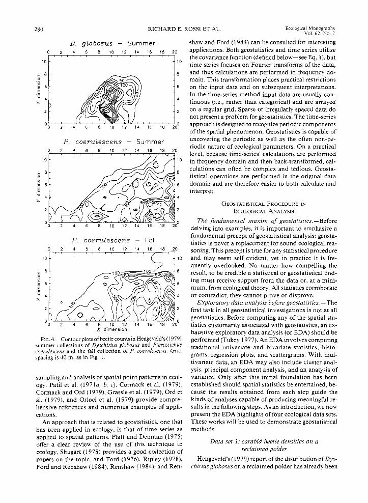
FIG. 4. Contour plots ofbeetle counts in Hengeveld’s (1 979) summer collections of Dyschirius globosus and Pterostichus cnerulescens and the fall collection of P. coerulescens. Grid spacing is 40 m. as in Fig. 1.
sampling and analysis of spatial point patterns in ecol- ogy. Patil et al. (1 97 1 a, 6 , c) , Cormack et al. (1 979), Cormack and Ord (1 979), Grassle et al. (1 979), Ord et al. (1979), and Orloci et al. (1979) provide compre- hensive references and numerous examples of appli- cations.
An approach that is related to geostatistics, one that has been applied in ecology, is that of time series as applied to spatial patterns. Platt and Denman (1975) offer a clear review of the use of this technique in ecology, Shugart (1978) provides a good collection of papers on the topic, and Ford (1976), Ripley (1978), Ford and Renshaw (1 984), Renshaw (1 984), and Ren-
shaw and Ford (1 984) can be consulted for interesting applications. Both geostatistics and time series utilize the covariance function (defined below-see Eq. l), but time series focuses on Fourier transforms of the data, and thus calculations are performed in frequency do- main. This transformation places practical restrictions on the input data and on subsequent interpretations. In the time-series method input data are usually con- tinuous (i.e., rather than categorical) and are arrayed on a regular grid. Sparse or irregularly spaced data do not present a problem for geostatistics. The time-series approach is designed to recognize periodic components of the spatial phenomenon. Geostatistics is capable of uncovering the periodic as well as the often non-pe- riodic nature of ecological parameters. On a practical level, because time-series’ calculations are performed in frequency domain and then back-transformed, cal- culations can often be complex and tedious. Geosta- tistical operations are performed in the original data domain and are therefore easier to both calculate and interpret.
GEOSTATISTICAL PROCEDURE IN
ECOLOGICAL ANALYSIS The fundamental maxim of geostatistics. -Before
delving into examples, it is important to emphasize a fundamental precept of geostatistical analysis: geosta- tistics is never a replacement for sound ecological rea- soning. This precept is true for any statistical procedure and may seem self evident, yet in practice it is fre- quently overlooked. No matter how compelling the result, to be credible a statistical or geostatistical find- ing must receive support from the data or, at a mini- mum, from ecological theory. All statistics corroborate or contradict; they cannot prove or disprove.
Exploratory data analysis before geostatistics. -The first task in all geostatistical investigations is not at all geostatistics. Before computing any of the spatial sta- tistics customarily associated with geostatistics, an ex- haustive exploratory data analysis (or EDA) should be performed (Tukey 1977). An EDA involves computing traditional univariate and bivariate statistics, histo- grams, regression plots, and scattergrams. With mul- tivariate data, an EDA may also include cluster anal- ysis, principal component analysis, and an analysis of variance. Only after this initial foundation has been established should spatial statistics be entertained, be- cause the results obtained from each step guide the kinds of analyses capable of producing meaningful re- sults in the following steps. As an introduction, we now present the EDA highlights of four ecological data sets. These works will be used to demonstrate geostatistical methods.
Data set 1: carabid beetle densities on a reclaimed polder
Hengeveld’s (1 979) report of the distribution of Dys- chirius globosus on a reclaimed polder has already been
June 1992 GEOSTATISTICAL TOOLS FOR ECOLOGY 28 1
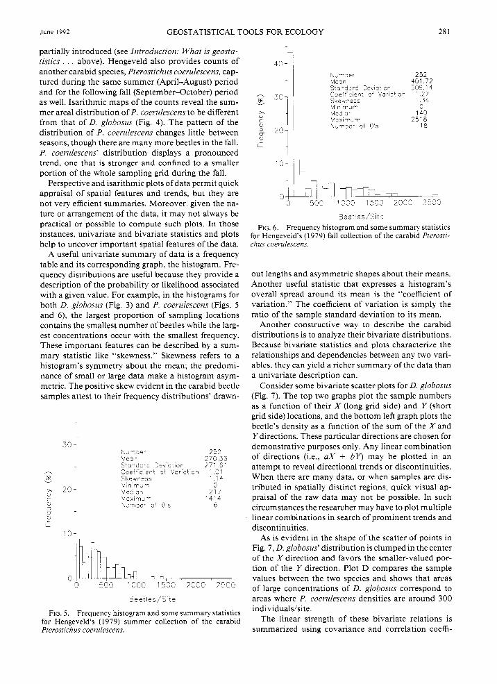
partially introduced (see Introduction: What is geosta- tistics . . . above). Hengeveld also provides counts of another carabid species, Pterostichus coerulescens, cap- tured during the same summer (April-August) period and for the following fall (September-October) period as well. Isarithmic maps of the counts reveal the sum- mer areal distribution of P. coerulescens to be different from that of D. glcbosus (Fig. 4). The pattern of the distribution of P. coerulescens changes little between seasons, though there are many more beetles in the fall. P. coerulescens’ distribution displays a pronounced trend, one that is stronger and confined to a smaller portion of the whole sampling grid during the fall.
Perspective and isarithmic plots of data permit quick appraisal of spatial features and trends, but they are not very efficient summaries. Moreover, given the na- ture or arrangement of the data, it may not always be practical or possible to compute such plots. In those instances, univariate and bivariate statistics and plots help to uncover important spatial features of the data.
A useful univariate summary of data is a frequency table and its corresponding graph, the histogram. Fre- quency distributions are useful because they provide a description of the probability or likelihood associated with a given value. For example, in the histograms for both D. globosus (Fig. 3 ) and P. coerulescens (Figs. 5 and 6), the largest proportion of sampling locations contains the smallest number of beetles while the larg- est concentrations occur with the smallest frequency. These important features can be described by a sum- mary statistic like “skewness.” Skewness refers to a histogram’s symmetry about the mean; the predomi- nance of small or large data make a histogram asym- metric. The positive skew evident in the carabid beetle samples attest to their frequency distributions’ drawn-
k u r r o e r 2 5 2 U e a n 2 7 0 . 3 6 S t a -, c c r c 2 ev i c : i o P 2 7 1 . 6 1 Coef’icient o f Var ic t ion 1 .01 Skewpess 1.14 L1 i n ’ r r L r r 0 L1 e c i a -, 2 1 7 U c x i m u m 1414 \Lrn>er o f 0 ’ s 6
I -
-
A- r r I ’
3 530 1033 1500 2330 2530
Beet les /S l te
FIG. 5 . Frequency histogram and some summary statistics for Hengeveld’s (1 979) summer collection of the carabid Pterostichus coerulescens.
I r 40 4
2 5 2 kLm3er Wean 4 0 1 . 7 2 S ta - ,da rc Deviation 509.1 4 Coeff ic ient of Variation 1 . 2 7 Skew-ess 1.34 M i n i r r u m 0 Med ian 140 W 3 X i r r L r r 2 5 1 8 \ u r r o e r o f 0 s 1 8
FIG. 6. Frequency histogram and some summary statistics for Hengeveld’s (1979) fall collection of the carabid Pterostr- chus coerulescens.
out lengths and asymmetric shapes about their means. Another useful statistic that expresses a histogram’s overall spread around its mean is the “coefficient of variation.” The coefficient of variation is simply the ratio of the sample standard deviation to its mean.
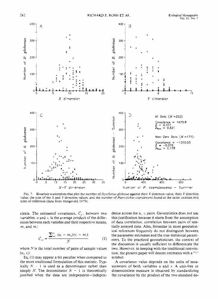
Another constructive way to describe the carabid distributions is to analyze their bivariate distributions. Because bivariate statistics and plots characterize the relationships and dependencies between any two vari- ables, they can yield a richer summary of the data than a univariate description can.
Consider some bivariate scatter plots for D. globosus (Fig. 7). The top two graphs plot the sample numbers as a function of their X (long grid side) and Y (short grid side) locations, and the bottom left graph plots the beetle’s density as a function of the sum of the X and Y directions. These particular directions are chosen for demonstrative purposes only. Any linear combination of directions (i.e., aX + b Y ) may be plotted in an attempt to reveal directional trends or discontinuities. When there are many data, or when samples are dis- tributed in spatially distinct regions, quick visual ap- praisal of the raw data may not be possible. In such circumstances the researcher may have to plot multiple linear combinations in search of prominent trends and discontinuities.
As is evident in the shape of the scatter of points in Fig. 7 , D. globosus’ distribution is clumped in the center of the X direction and favors the smaller-valued por- tion of the Y direction. Plot D compares the sample values between the two species and shows that areas of large concentrations of D. globosus correspond to areas where P. coerulescens densities are around 300 individuals/site.
The linear strength of these bivariate relations is summarized using covariance and correlation coeffi-
2 8 2
400 -
2 300- 0 9
03 u
s' 200-
RICHARD E. ROSS1 ET AL.
B
Ecological Monographs Vol. 6 2 , No. 2
A
3 300
u 03
x
X dimension
u 03 300i x n
I
u 03 300\ x n
L 9 2oo;
L
0
L
Y dimension
4001 D All Data ( N =252): ??
Covariance = 1673.8 = 0.107
t E Ln 300 P R ~ ~ ~ = 0.621
m Non-Zero Data ( N =171):
Covariance = - 131 0.03 p^ = -0.076 /5R0"k = 0.138 200
u 03
s' E 100
Z a n E
L
Z 0
0 5 10 15 20 25 30 35 0 400 800 1200
X+Y dimension Number of P. coerulescens - Summer
FIG. 7. Bivariate scatterplots that plot the number of Dyschirius globosus against their X direction value, their Y direction value, the sum of the X and Y direction values, and the number of Pterostichus coerulescens found at the same location and time of collection (data from Hengeveld 1979).
cients. The estimated covariance, 6,,, between two variables, u and v, is the average product of the differ- ences between each variable and their respective means, m,, and m,:
where N is the total number of pairs of sample values
Eq. (1) may appear a bit peculiar when compared to the more traditional formulation of this statistic. Typ- ically N - 1 is used as a denominator rather than simply N. The denominator N - 1 is theoretically justified when the data are independent- indepen-
(u,, v,).
dence across the u,, v, pairs. Geostatistics does not use this justification because it starts from the assumption of data correlation, correlation between pairs of spa- tially arrayed data. Also, formulae in most geostatist- ical references frequently do not distinguish between the parameter estimates and the true statistical param- eters. To the practiced geostatistician, the context of the discussion is usually sufficient to differentiate the two. However, in keeping with the traditional conven- tion, the present paper will denote estimates with a ''h"
symbol. A covariance value depends on the units of mea-
surement of both variables u and v. A unit-free or dimensionless measure is obtained by standardizing the covariance by the product of the two standard de-
June 1992 GEOSTATISTICAL TOOLS FOR ECOLOGY 283
AIi D a t a Y o r - Z e r o Data N 252 233
3330, Eovar o r c e 121,773 122,573 ~ 0 887 0 883 0
LL 3 932 0 916 F,
O + V k -
I
2330 4
I 1230 1600
Nu-nber o4 P c o e r u l e s c e n s - Su-n-ne.
FIG. 8. Bivariate scatterplot that plots the numbers of Pterostichus coerulescens found dunng the fall collection vs. the number found during the summer collection (data from Hengeveld 1979).
viations. The resulting statistic is known as the esti- mated Pearson product-moment or the linear corre- lation coefficient:
The Pearson correlation coefficient measures how well one variable can be represented as a linear function of the other. This statistic can range from - 1 to + 1 de- pending on whether the variables are related linearly in a negative or positive manner; a score of - 1 cor- responds to perfect negative linear correlation and + 1 to perfect positive linear correlation. A +0.107 correlation between the two beetles suggests a very low positive linear relationship exists between their densities (see Fig. 7).
Nevertheless, the two variables u and v could be highly dependent without being linearly related, a clas- sic example being: u = v2. A measure of monotonic dependence, whether linear or not, is the "Spearman rank correlation" (Davis 1986). The Spearman rank correlation is none other than the linear correlation coefficient of the data's ranks. For instance, sample u, has rank R,,, and is equal to 1 if it is the smallest value and N if it is the largest value of u. Similarly, the corresponding sample v, has rank R,!. The Spearman rank correlation coefficient is thus defined as:
;Ron& = (3) N S R ~ R ,
where mRu and mR, are the means of the ranks of the
u and v values, and sR,, and sR, are the standard devi- ations of the ranks of the u and v values.
Notice that when comparing D. globosus and P. coe- rulescens densities, the Spearman correlation coeffi- cient is different from the Pearson correlation coeffi- cient. The small Pearson but large Spearman statistics suggest that the relationship between D. globosus and the co-occurring P. coerulescens beetle could be non- linear.
However, this comparison pairs locations where no beetles are present for one species with those where the other species does exist. Namelq, there are 8 1 D. glo- bosus locations and 6 P. coerulescens locations where no beetles of the other species were present. Another way to analyze the data is to compare only those lo- cations that actually contain both beetles. When these latter locations are analyzed, the Pearson statistic be- comes -0.076 and the Spearman statistic an incon- sequential 0.138. Thus, the relationship between the two co-occurring beetles is apparently neither linear nor monotonic.
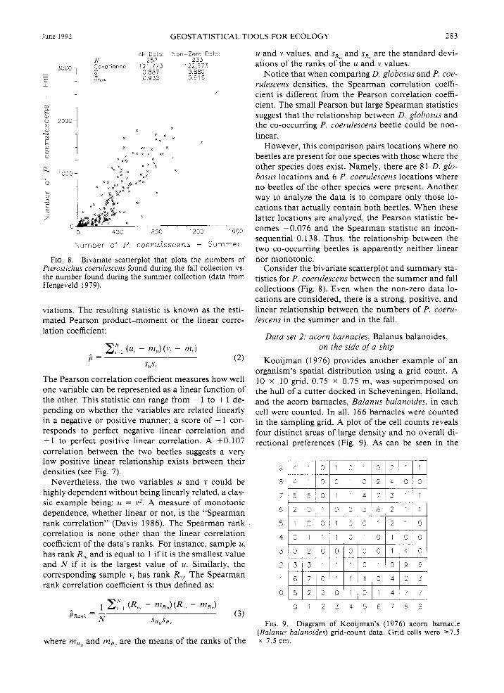
Consider the bivariate scatterplot and summary sta- tistics for P. coerulescens between the summer and fall collections (Fig. 8). Even when the non-zero data lo- cations are considered, there is a strong, positive, and linear relationship between the numbers of P. coeru- lescens in the summer and in the fall.
Data set 2: acorn barnacles, Balanus balanoides, on the side of a ship
Kooijman ( 1 976) provides another example of an organism's spatial distribution using a grid count. A 10 x 10 grid, 0.75 x 0.75 m, was superimposed on the hull of a cutter docked in Scheveningen, Holland, and the acorn barnacles, Balanus balanoides, in each cell were counted. In all, 166 barnacles were counted in the sampling grid. A plot of the cell counts reveals four distinct areas of large density and no overali di- rectional preferences (Fig. 9). As can be seen in the
' 0 1 2 3 4 5 5 7 5 9
FIG. 9. Diagram of Kooijman's (1976) acorn barnacle (Balanus balanoides) grid-count data. Grid cells were ~ 7 . 5 x 7.5 cm.
284 RICHARD E. ROSS1 ET AL. Ecological Monographs Vol. 62, No. 2
43 -
- -
Me- i cn Mc x , m J T, Num>e, 0' 3 s
100 1.66
. 27 1.59 0 1 9
35
? . l o
l ! l I I , I '
- 1 n 1 2 3 4 5 6 7 9 9 '24 , ~ ,
3 0 ~ 1 o c es /Ce l l
FIG. 10. Frequency histogram and some summary statis- tics for Kooijman's (1976) data presented in Fig. 9.
histogram for these data (Fig. lo), > 60 of the 100 cells contain either one or no barnacles while two of the cells are populated with the largest (8 and 9) densities of barnacles. The large proportion of small or no bar- nacles is reflected in the distribution's strong positive skew.
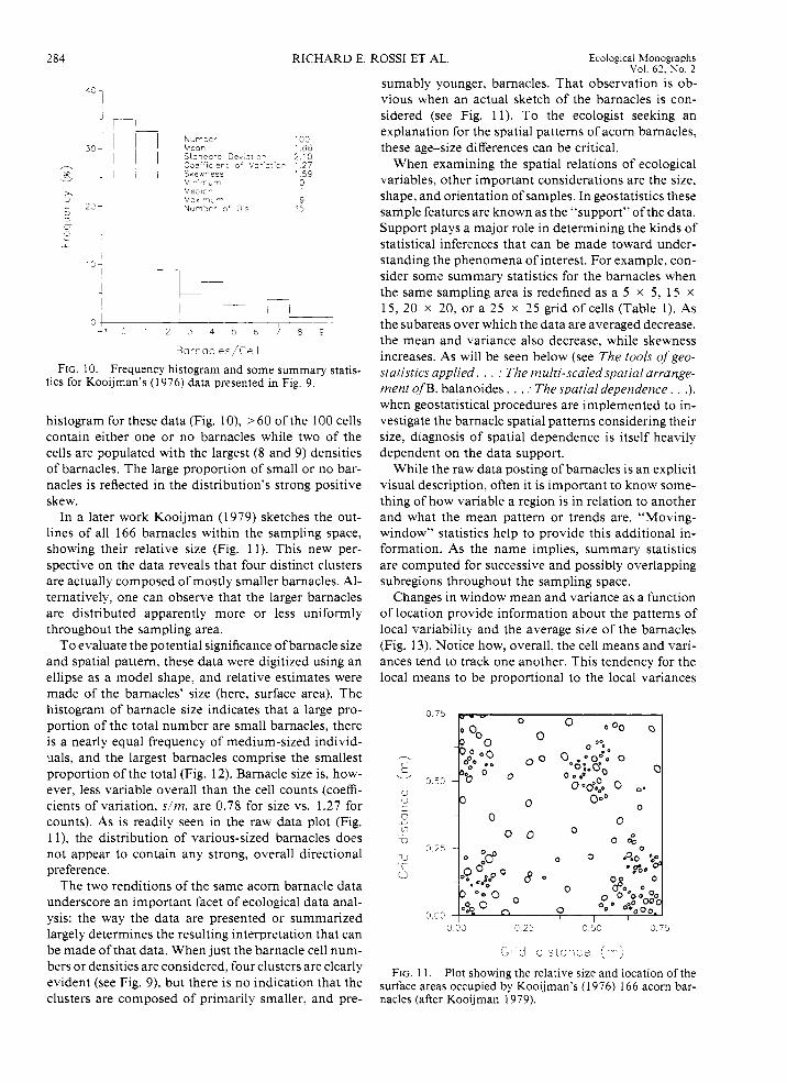
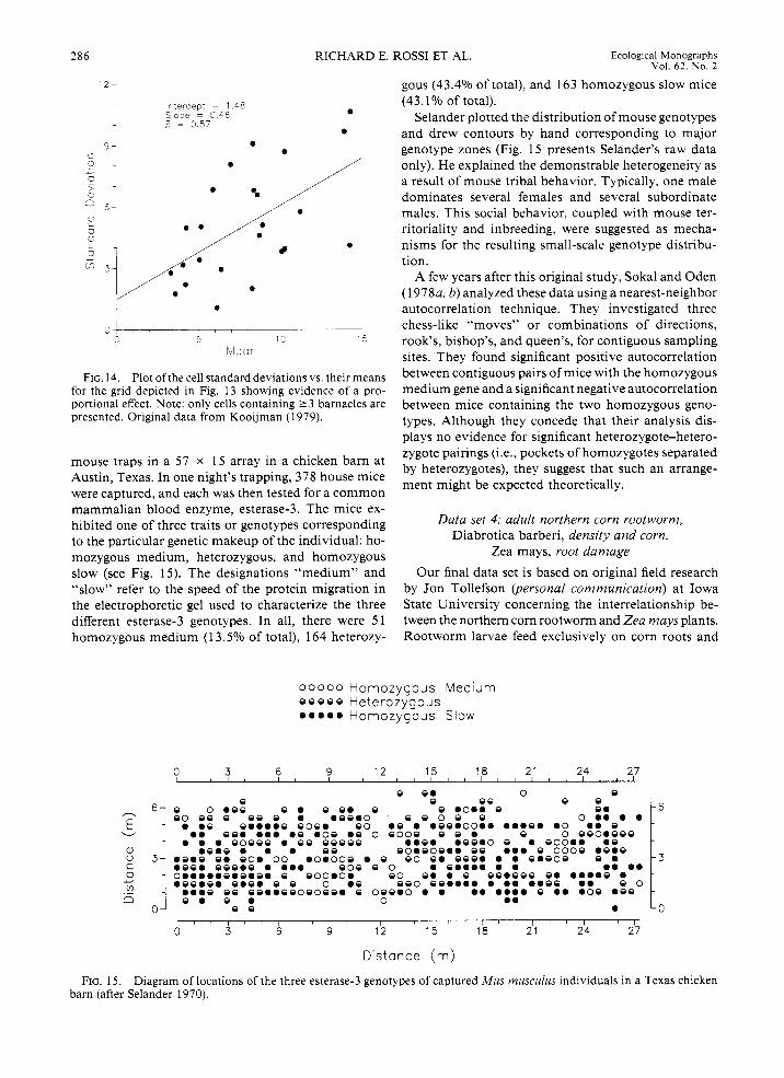
In a later work Kooijman (1979) sketches the out- lines of all 166 barnacles within the sampling space, showing their relative size (Fig. 11). This new per- spective on the data reveals that four distinct clusters are actually composed of mostly smaller barnacles. Al- ternatively, one can observe that the larger barnacles are distributed apparently more or less uniformly throughout the sampling area.
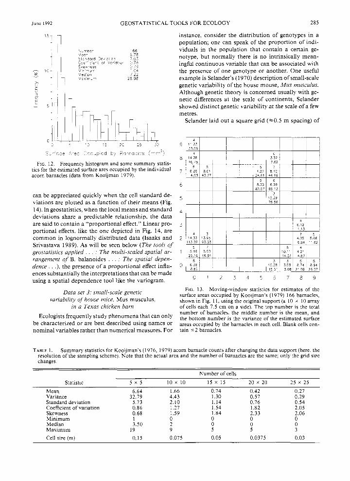
To evaluate the potential significance of barnacle size and spatial pattern, these data were digitized using an ellipse as a model shape, and relative estimates were made of the barnacles' size (here, surface area). The histogram of barnacle size indicates that a large pro- portion of the total number are small barnacles, there is a nearly equal frequency of medium-sized individ- iials, and the largest barnacles comprise the smallest proportion of the total (Fig. 12). Barnacle size is, how- ever, less variable overall than the cell counts (coeffi- cients of variation, slm, are 0.78 for size vs. 1.27 for counts). As is readily seen in the raw data plot (Fig. 1 l) , the distribution of various-sized barnacles does not appear to contain any strong, overall directional preference.
The two renditions of the same acorn barnacle data underscore an important facet of ecological data anal- ysis: the way the data are presented or summarized largely determines the resulting interpretation that can be made of that data. When just the barnacle cell num- bers or densities are considered, four clusters are clearly evident (see Fig. 9), but there is no indication that the clusters are composed of primarily smaller, and pre-
sumably younger, barnacles. That observation is ob- vious when an actual sketch of the barnacles is con- sidered (see Fig. 11). To the ecologist seeking an explanation for the spatial patterns of acorn barnacles, these age-size differences can be critical.
When examining the spatial relations of ecological variables, other important considerations are the size, shape, and orientation of samples. In geostatistics these sample features are known as the "support" of the data. Support plays a major role in determining the kinds of statistical inferences that can be made toward under- standing the phenomena of interest. For example, con- sider some summary statistics for the barnacles when the same sampling area is redefined as a 5 x 5, 15 x 15, 20 x 20, or a 25 x 25 grid of cells (Table 1). As the subareas over which the data are averaged decrease, the mean and variance also decrease, while skewness increases. As will be seen below (see The tools of geo- statistics applied. . . : The multi-scaled spatial arrange- ment of B. balanoides . . . : The spatial dependence. . .), when geostatistical procedures are implemented to in- vestigate the barnacle spatial patterns considering their size, diagnosis of spatial dependence is itself heavily dependent on the data support.
While the raw data posting of barnacles is an explicit visual description, often it is important to know some- thing of how variable a region is in relation to another and what the mean pattern or trends are. "Moving- window" statistics help to provide this additional in- formation. As the name implies, summary statistics are computed for successive and possibly overlapping subregions throughout the sampling space.
Changes in window mean and variance as a function of location provide information about the patterns of local variability and the average size of the barnacles (Fig. 13). Notice how, overall, the cell means and vari- ances tend to track one another. This tendency for the local means to be proportional to the local variances
0 c 3 0 25 0.5c 3 .75
FIG. 1 1. Plot showing the relative size and location of the surface areas occupied by Kooijman's ( 1 976) 166 acorn bar- nacles (after Kooijman 1979).
June 1992 GEOSTATISTICAL TOOLS FOR ECOLOGY 285
U 8” n be r Mec- S t c - d a r d D e v a t i o - C o e f f ’ c ’ e n t o f Var ia t oq Skew-ess M n i n J n Med c n N c x rrrn
166 E 78 7.63 C 75
04 7 22
2E 98
; 79
3c
S;’-P- i”c Arec Cce-p led by 3 a r I o c es (TI-‘:
FIG. 12. Frequency histogram and some summary statis- tics for the estimated surface ares occupied by the individual acorn barnacles (data from Kooijman 1979).
can be appreciated quickly when the cell standard de- viations are plotted as a function of their means (Fig. 14). In geostatistics, when the local means and standard deviations share a predictable relationship, the data are said to contain a “proportional effect.” Linear pro- portional effects, like the one depicted in Fig. 14, are common in lognormally distributed data (Isaaks and Srivastava 1989). As will be seen below (The tools of geostatistics applied . . . : The multi-scaled spatial ar- rangement of B. balanoides . . . : The spatial depen- dence . . .), the presence of a proportional effect influ- ences substantially the interpretations that can be made using a spatial dependence tool like the variogram.
Data set 3: small-scale genetic variability of house mice, Mus musculus,
in a Texas chicken barn Ecologists frequently study phenomena that can only
be characterized or are best described using names or nominal variables rather than numerical measures. For
instance, consider the distribution of genotypes in a population; one can speak of the proportion of indi- viduals in the population that contain a certain ge- notype, but normally there is no intrinsically mean- ingful continuous variable that can be associated with the presence of one genotype or another. One useful example is Selander’s (1 970) description of small-scale genetic variability of the house mouse, Mus musculus. Although genetic theory is concerned usually with ge- netic differences at the scale of continents, Selander showed distinct genetic variability at the scale of a few metres.
Selander laid out a square grid ( ~ 0 . 5 m spacing) of
0 ? 2 3 4 5
65.13
10.29
6 7 8 9
FIG. 13. Moving-window statistics for estimates of the surface areas occupied by Kooijman’s (1 979) 166 barnacles, shown in Fig. 1 1, using the original support (a 10 x 10 array of cells each 7.5 cm on a side). The top number is the total number of barnacles, the middle number is the mean, and the bottom number is the variance of the estimated surface areas occupied by the barnacles in each cell. Blank cells con- tain 5 2 barnacles.
TABLE 1. Summary statistics for Kooijman’s (1976, 1979) acorn barnacle counts after changing the data support (here, the resolution of the sampling scheme). Note that the actual area and the number of barnacles are the same; only the grid size changes.
Number of cells _ _ _ _ _ _ _ _ _ ~ ~
Statistic 5 x 5 10 x 10 15 x 15 20 x 20 25 x 25
Mean 6.64 1.66 0.74 0.42 0.27 Variance 32.79 4.43 1.30 0.57 0.29 Standard deviation Coefficient of variation Skewness Minimum Median Maximum Cell size fm)
5.73 2.10 1.14 0.76 0.54 0.86 1.27 1.54 1.82 2.05 0.68 1.59 1.84 2.33 2.06 1 0 0 0 0 3.50 2 0 0 0
19 9 5 5 3
0.15 0.075 0.05 0.0375 0.03
286 RICHARD E. ROSS1 ET AL. Ecological Monographs Vol. 62. No. 2
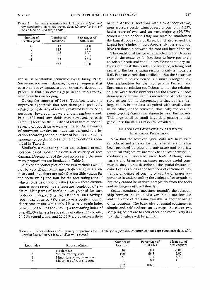
' 2 - gous (43.4% of total), and 163 homozygous slow mice (43.1% of total).
Selander plotted the distribution of mouse genotypes and drew contours by hand corresponding to major genotype zones (Fig. 15 presents Selander's raw data
1r:ercep: = 1 48 S c z e = 3 46 5 = 3.57
only). He explained the demonstrable heterogeneity as a result of mouse tribal behavior. Typically, one male dominates several females and several subordinate males. This social behavior, coupled with mouse ter- ritoriality and inbreeding, were suggested as mecha- nisms for the resulting small-scale genotype distribu- tion.
A few years after this original study, Sokal and Oden (1 978a, b) analyzed these data using a nearest-neighbor autocorrelation technique. They investigated three
I chess-like "moves" or combinations of directions, 12 ' 5 rook's, bishop's, and queen's, for contiguous sampling
sites. They found significant positive autocorrelation between contiguous pairs Of mice with the homozygous medium gene and a significant negative autocorrelation between mice containing the two homozygous geno- types. Although they concede that their analysis dis- plays no evidence for significant heterozygote-hetero- zygote pairings (i.e., pockets of homozygotes separated by heterozygotes), they suggest that such an arrange- ment might be expected theoretically.
i -
I " "
1.,1 ec f I
FIG. 14. Plot ofthe cell standard deviations vs. their means for the grid depicted in Fig, 13 showing evidence of a pro- portional effect. Note: only cells containing 2 3 barnacles are presented. Original data from Kooijman ( 1 979).
mouse traps in a 57 x 15 array in a chicken barn at Austin, Texas. In one night's trapping, 378 house mice were captured, and each was then tested for a common
6 - - -
3 2 - -
0-
mammalian blood enzyme, esterase-3. The mice ex- hibited one of three traits or genotypes corresponding to the particular genetic makeup of the individual: ho- mozygous medium, heterozygous, and homozygous slow (see Fig. 15). The designations "medium" and "slow" refer to the speed of the protein migration in the electrophoretic gel used to characterize the three different esterase-3 genotypes. In all, there were 51 homozygous medium (1 3.5% of total), 164 heterozy-
0 0. 0 0 0 8 8 0 0
o o 09: 0 . 8 8 . 0 0 .0.. 0 0. 80 8 8 0 8 8 0 0 088.0 0 0 0 0 0 O....
0 0 8 8....8 808. 80 0 8 0 .88.00.. ...0. 0 0 0. 0 0. 8 8 . 0.. 0 8 008 0 8 0 0000 0 0 0 0 0 880.888
0 0 0 0 0 0 0 8 0 8 8 0 0 0 0 8 ..0. 088.0 0 0 800.. 0 8 08.8 0 0 0 8 8 80.808.. 8 8 0.. 0 0 0 0 8 .8.8
.8.8 0. 80. 00 .0.008 0 0 80 0. 888 . 0 0 8.808 0 0
.88. 888.8 0 0.. 808 0 0 0 0.... 0 0 0. 0. 0.....8.8.8. 0 800.0. 80 0 . 0 0 88.888 0. ....O 0 088.8. 8.8. 0 0 0 0 8 880 88.... 0 0. ..88 0. 0 0
00.8 8 8 88..8808088. 0 088.0 0 0 0. .... 0 0. 008 0 8 8 0 . 0 0 0 0 .
8 8 0
Data set 4: adult northern corn rootworm, Diabrotica barberi, density and corn,
Zea mays, root damage Our final data set is based on original field research
by Jon Tollefson (personal communication) at Iowa State University concerning the interrelationship be- tween the northern corn rootworm and Zea mays plants. Rootworm larvae feed exclusively on corn roots and
- 6
- 3
-0
0 0 0 0 0 HomozygoJs MediJrn o o o o o Heterozygous ..... Homozygous Slow
0 m Y
.- n
Distance (m) FIG. 15. Diagram of locations of the three esterase-3 genotypes of captured Mus musculus individuals in a Texas chicken
barn (after Selander 1970).
June 1992 GEOSTATISTICAL TOOLS FOR ECOLOGY 287
TABLE 2. Summary statistics for J. Tollefson’s (personal communication) corn rootworm data. (Diabrotrca barberi larvae feed on Zea mays roots.)
Number of Number of Percentage of beetleslplant locations total sites
0 13 1 113 2 48 3 55
2 4 43 272
4.8 41.5 17.7 20.2 15.8
100.0
can cause substantial economic loss (Chiang 1973). Surveying rootworm damage, however, requires that corn plants be extirpated, a labor-intensive, destructive procedure that also creates gaps in the crop canopy, which can hasten lodging.
During the summer of 1988, Tollefson tested the unproven hypothesis that root damage is positively related to the density of recently matured beetles. Nine northwest Iowa counties were chosen randomly and, in all, 272 total corn fields were surveyed. At each sampling location the number of adult beetles and the severity of root damage were estimated. As a measure of rootworm density, an index was assigned to a lo- cation according to the number of beetles counted. A summary of beetle indices and their proportions is pro- vided in Table 2.
Similarly, a root-rating index was assigned to each location based upon the extent and severity of root damage. Descriptions of the root indices and the sum- mary proportions are itemized in Table 3.
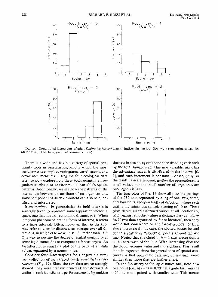
A bivariate scatter plot of these two variables would not be very illuminating since both variables are in- dices, and thus there are only five possible values for the beetle rating and four for the root rating (one of which contains only one value). Given these circum- stances, more revealing statistics are “conditional” sta- tistics: histograms of beetle indices graphed for each root-index category (Fig. 16). Of the 50 sites having a root index of zero, 98% also have a beetle index of eiiher zero or one while only 2% score a beetle index of two. For the 190 sites having a root-rating index of one, 40.53% have a beetle rating of either zero or one, 24.2 1% scored a two, and 25.26% scored either a three
or four. At the 31 locations with a root index of two, none scored a beetle rating of zero or one, only 3.23% had a score of two, and the vast majority (96.77%) scored a three or four. Only one location manifested the largest root rating of three, but it also scored the largest beetle index of four. Apparently, there is a pos- itive relationship between the root and beetle indices.
The conditional histograms depicted in Fig. 16 make explicit the tendency for locations to have positively correlated beetle and root indices. Some summary sta- tistics can mask this result. For instance, relating root rating to the beetle rating results in only a moderate 0.63 Pearson correlation coefficient. But the Spearman rank correlation coefficient is a much stronger 0.89. One explanation for the incongruous Pearson and Spearman correlation coefficients is that the relation- ship between beetle numbers and the severity of root damage is nonlinear, yet it is monotonic. Another pos- sible reason for the discrepancy is that outliers (i.e., large values in one data set paired with small values in the other, or the converse) drastically reduces the point-to-point Pearson correlation between the two sets. This large-small or small-large data pairing is miti- gated once the data’s ranks are considered.
THE TOOLS OF GEOSTATISTICS APPLIED TO ECOLOGICAL PHENOMENA
Now that the four ecological data sets have been introduced and a flavor for their spatial relations has been provided by plots and univariate and bivariate statistical analyses, we are ready to analyze their spatial continuity with more-advanced tools. Although uni- variate and bivariate measures provide useful sum- maries, they do not describe all the spatial features of data. Features such as the locations of extreme values, trends, or degree of continuity can be of major im- portance in understanding the ecology of an organism, but they cannot be derived completely from the tools and techniques utilized thus far.
Spatial continuity measures quantify the relation- ship between the value of a variable at one location and the value of the same variable or another one at other locations. The basic idea of spatial continuity is simple and self-evident: on average, the closer two sampling points are to each other, the more likely it is that their values will be similar.
TABLE 3. Root indices and summary proportions for J. Tollefson’s (personal communication) corn rootworm data. (Dia- brotica barberi larvae feed on Zea mays roots.)
Number of Percentage of Mean no. of locations total sites beetledplant Root index Root condition
0 No damage 50 18.4 0.86
2 Minor loss of root structure 31 11.4 3.71 1 Visible feeding scars 190 69.8 2.02
3 Major loss of root structure 1 0.4 4 272 100.0
288 RICHARD E. ROSS1 ET AL Ecological Monographs Vol. 62, No. 2
Root Index = 0 (N=50)
J - -7
201 I I ,
- 1 0 i i j i Beet le Index
O - 1 0 1 2 3 4 B e e t e Index
201 1 , r h O - 1 0 1 2 3 4 0-
- 1 0
m I 1 2 3 4
Beet le Index
Rgot Index = 3 lO0l ( N = 1 )
6 i e i B e e t e Index
5
7 5
FIG. 16. Conditional histograms of adult Diabrotica barberi density indices for the four Zea mays root-rating categories (data from J. Tollefson, personal communication).
There is a wide and flexible variety of spatial con- tinuity tools in geostatistics, among which the most useful are h-scatterplots, variograms, correlograms, and covariance measures. Using the four ecological data sets, we now explore how these tools quantify an or- ganism attribute or environmental variable’s spatial patterns. Additionally, we see how the patterns of the interaction between an attribute of an organism and some component of its environment can also be quan- tified and interpreted.
h-scatterplots. -In geostatistics the bold letter h is generally taken to represent some separation vector in space, one that has a direction and distance to it. When temporal phenomena are the focus of interest, h refers to a time interval. Often, however, the lag distance may refer to a scalar distance, an average over all di- rections, in which case we will use “h” rather than “h.” One way to portray the degree of spatial continuity at some lag distance h is to compute an h-scatterplot. An h-scatterplot is simply a plot of the pairs of all data values separated by a common lag.
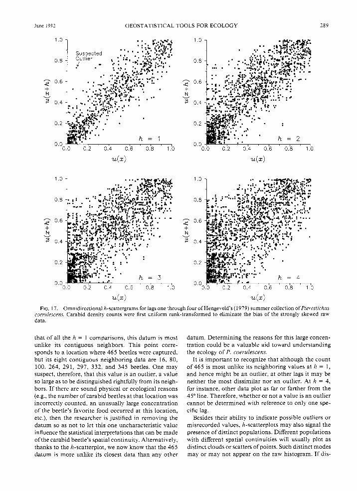
Consider four h-scatterplots for Hengeveld’s sum- mer collection of the carabid beetle Pterostichus coe- rulescens (Fig. 17). Since the raw data are so strongly skewed, they were first uniform-rank transformed. A uniform-rank transform is performed easily by ranking
the data in ascending order and then dividing each rank by the total sample size. This new variable, u(x), has the advantage that it is distributed in the interval [0, 11, and each increment is constant. Consequently, in the resulting h-scattergram, neither the preponderating small values nor the small number of large ones are privileged visually.
The four plots of Fig. 17 show all possible pairings of the 2 5 2 data separated by a lag of one, two, three, and four units, independently of direction, where each unit is the minimum sample spacing of 40 m. These plots depict all transformed values at all locations x, u(x), against all other values a distance h away, u(x + h). If two data separated by h are identical, then they would fall somewhere on the h-scatterplot’s 45” line. Since this is rarely the case, the plotted points instead define a scatter or “cloud” of points around the 45” line. Notice that the cloud of h = 1 scatterplot points is the narrowest of the four. With increasing distance the cloud becomes wider and more diffuse. This result is to be expected since the general idea of spatial con- tinuity is that proximate data are, on average, more similar than those that are farther apart.
In the h-scatterplot for lag distance one, note how one point [i.e., u(x+h) 2: 0.731 falls quite far from the 45” line when paired with smaller data. This means
June 1992 GEOSTATISTICAL TOOLS FOR ECOLOGY 289
' . O 1 .... 1 Susoected
. .
1 ---T-
0.2 0.4 0.'6 0.8 1 . 0
H 3
W
FIG. 17. Omnidirectional h-scattergrams for lags one through four of Hengeveld's ( 1 979) summer collection of Pterostichus coerulescens. Carabid density counts were first uniform rank-transformed to eliminate the bias of the strongly skewed raw data.
that of all the h = 1 comparisons, this datum is most mlike its contiguous neighbors. This point corre- sponds to a location where 465 beetles were captured, but its eight contiguous neighboring data are 16, 80, 100, 264, 291, 297, 332, and 345 beetles. One may suspect, therefore, that this value is an outlier, a value so large as to be distinguished rightfully from its neigh- bors. If there are sound physical or ecological reasons (e.g., the number of carabid beetles at that location was incorrectly counted, an unusually large concentration of the beetle's favorite food occurred at this location, etc.), then the researcher is justified in removing the datum so as not to let this one uncharacteristic value influence the statistical interpretations that can be made of the carabid beetle's spatial continuity. Alternatively, thanks to the h-scatterplot, we now know that the 465 datum is more unlike its closest data than any other
datum. Determining the reasons for this large concen- tration could be a valuable aid toward understanding the ecology of P. coerulescens.
It is important to recognize that although the count of 465 is most unlike its neighboring values at h = 1, and hence might be an outlier, at other lags it may be neither the most dissimilar nor an outlier. At h = 4, for instance, other data plot as far or farther from the 45" line. Therefore, whether or not a value is an outlier cannot be determined with reference to only one spe- cific lag.
Besides their ability to indicate possible outliers or misrecorded values, h-scatterplots may also signal the presence of distinct populations. Different populations with different spatial continuities will usually plot as distinct clouds or scatters of points. Such distinct modes may or may not appear on the raw histogram. If dis-
290 RICHARD E. ROSS1 ET AL. Ecological Monographs Vol. 6 2 . No. 2
TABLE 4. Summary statistics for Pterostichus coerulescens’ four h-scatterplots shown in Fig. 17.
Lag covanance Moment
(no. of Correlation of inertia h beetles)2 coefficient (no./cell)2
1 59 757 0.862 9817 2 52 307 0.796 15 175 3 46 647 0.728 21 083 4 40 466 0.656 27 413
6ooc 1
I @’
Crete populations are suspected, the researcher should, data permitting, separate the distinct populations and analyze them separately for spatial continuity. Other- wise, an analysis on the mixture of populations may provide a misleading (i.e., merely average) portrait of the extant spatial relations.
Another advantage of h-scatterplots is that their asymmetry about the 45” line can signal trends or dif- ferences in the local means and variance. In the graphs in Fig. 17, for example, note how the small u(x) values plot disproportionately more often on the u(x + h) side of the 45” line. This asymmetry corresponds to comparisons between locations with small densities and those having larger densities of beetles. We have already seen that P. coerulescens’ density reflects a strong trend (see Fig. 4), so this feature is reflected in the h-scatterplot.
h-scatterplots are useful tools, but they fail to sum- marize precisely and succinctly spatial continuity. The degree of scatter or the size of the cloud in an h-scat- terplot can be summarized using the covariance (Eq. 1) or the correlation coefficient (Eq. 2) measures. The first two columns of Table 4 itemize the covariance and correlation coefficients for each of the four lag distances for P. coerulescens. Both the covariance and the degree of correlation decrease with increasing lag distance, and thus, as suspected, the data are more dissimilar the farther apart they are.
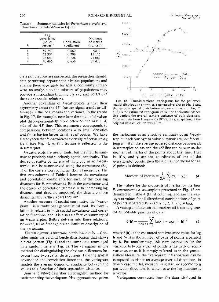
Another measure of spatial continuity, the “vario- gram,” is a traditional geostatistical tool. Its formu- lation is related to both spatial covariance and corre- lation functions, and it is also an effective summary of an h-scatterplot. Before delving into these relations, however, let us first explore an intuitive description of the variogram.
The variogram: a bivariate, statistical model. -Con- sider again the carabid beetle distribution that shows a clear pattern (Fig. 1) and the same data rearranged in a random pattern (Fig. 2). The variogram is one method for distinguishing the obvious differences be- tween these two spatial distributions. Like the spatial covariance and correlation functions, the variogram models the average degree of similarity between the values as a function of their separation distance.
Journel (1 984b) describes an insightful method for understanding the variogram. His approach recognizes
ooooo P a t t e r r e d 3a ta M+E Random 3 a t a
-I I
1 0 0 0 - 0
o ~ , , , I ’ , # , I 1 C 2 4 6 8 i 0 12
Lcg 3 ’ s t c n c e (40m J i ‘ t s )
FIG. 18. Omnidirectional variograms for the patterned spatial distribution shown as a perspective plot in Fig. 1 and the random spatial distribution shown similarly in Fig. 2. i. ( h ) is the estimated variogram value; the horizontal dashed line depicts the overall sample variance of both data sets. Original data from Hengeveld (1979); the grid spacing in the original data collection was 4 0 m.
the variogram as an effective summary of an h-scat- terplot: each variogram value summarizes one h-scat- tergram. Half the average squared distance between all h-scatterplot points and the 45” line can be seen as the moment of inertia of the points about that line. That is, if x, and y, are the coordinates of one of the h-scatterplot points, then the moment of inertia for all N points is defined:
. \ I
Moment of inertia = - (x, - yJ2. (4) 2N !=,
The values for the moments of inertia for the four P. coerulescens h-scatterplots presented in Fig. 17 are itemized in Table 4 (third column), and are the var- iogram values for all directional combinations of pairs of points separated by exactly 1 , 2, 3, and 4 lags.
A variogram function summarizes all h-scattergrams for all possible pairings of data:
where +(h) is the estimated semivariance value for lag h and N(h) is the number of pairs of points separated by h. Put another way, this new expression for the variance between a pair of points is the half- or semi- variance, or as it is simply referred to in the geosta- tistical literature: the “variogram.” Variograms can be computed as either an average over all directions, in which case the lag measure is scalar, or specific to a particular direction, in which case the lag measure is a vector.
Variograms computed from the data displayed in
June 1992 GEOSTATISTICAL TOOLS FOR ECOLOGY 29 1
Fig. 1 and Fig. 2 for all possible pairs of points over the sampling space are distinctly different (Fig. 18). For the random data all values are essentially the same, and thus the variogram appears nearly horizontal. The patterned data, on the other hand, produce a variogram that has small values for short lags, then increases with increasing distance, but levels off and even decreases after about lag nine. These features reflect the degree of spatial variability or, conversely, continuity in the data. Constant variogram values mean that, on aver- age, the variance between values does not change with distance. Small variogram values at short lags corre- spond to data that are closer together and more alike or more spatially continuous. Conversely, large var- iogram values reflect data that are farther apart and more dissimilar or spatially discontinuous.
Notice that the random pattern’s vanogram remains near the sample variance of 3369. A plot of these raw data demonstrated no detectable spatial continuity (see Fig. 2 ) , and this characteristic is reflected in the fairly constant variogram, one nearly equivalent to the over- all sample variance. In this instance the sample vari- ance suffices to summarize the spatial continuity at all lags. In contrast, the patterned data set’s variogram values summarize the degree of spatial variability ev- ident at each particular lag distance.
It should be pointed out that a variogram is a special type of model. Although a model is typically defined as a deterministic paradigm that explains or predicts, a variogram is a statistical model. It summarizes the samples’ two-point or bivariate relations, i.e., the av- erage squared difference between samples aligned in a particular direction and separated by some common lag. This observed or experimental variogram is a de- scriptive statistical model for the particular realization of the phenomenon under study. Because our sampling is limited, we assume, therefore, that our experimental variogram is representative of the true variogram had our sampling been exhaustive.
We have said that the variogram is a statistical model of spatial dependence. Traditionally, there are two types of spatial dependence: “structural” and “stochastic.” Structural spatial dependence refers to large-scale data trends and involves jointly several data locations. Sto- chastic spatial dependence refers to small scale corre- lation structures usually at distances smaller than the separation distance between two data locations. Al- though the distinction between the two types is scale dependent, the variogram models structural spatial de- pendence.
Credit is usually given to Matheron (1963, 1965), Journel and Huijbregts (1 978), and David (1 977) among many others in the field of mining geology for dem- onstrating the variogram’s practical use. To be sure, their works have advanced the use of the variogram as a spatial-continuity measure. Nevertheless, some years before mining geologists took note of the advan- tages of the variogram, biomathematicians Matern
(1947) and Jowett ( 1 955) used a “serial variation func- tion” identical to the variogram. Their application in- volved quantification of local or short-distance vs. long- distance variation and its effect on the proper design of sampling regimes. Matern (1 947) applied spatial cor- relation measures to the distribution of Swedish for- ests. Whittle’s (1 954, 1956, 1963) works, especially his 1963 text, foreshadowed much of the geostatistics that was later developed by Matheron and his associates in Fontainebleau, France. Some of the same can be said for Wold (1938), Kolmogorov (1941), Wiener (1949), Yaglom (1 957), Goldberger (1 962), and Gandin (1 963). But even these works were not among the oldest. Ma- tern (1 960) relates that the Swedish forester Langsaeter used what is essentially the variogram to express vari- ation in forest surveys as early as 1926.
Now that the idea of a variogram and a bit of its biological heritage has been developed, let us re-ex- amine this old tool using the four ecological data sets. In addition, we also explore some other related, but often more revealing and dependable, spatial-conti- nuity tools. Most of the spatial-continuity tools will be presented using Hengeveld’s (1 979) carabid beetle data. These data are best suited to introduce the tools be- cause the spatial patterns of the carabids are readily apparent in the raw data plots (Fig. 4), so interpretation using these new tools is more quickly grasped. This will be a distinct advantage later when the spatial pat- terns of other organisms are investigated-organisms whose spatial patterns are not as visually obvious.
The spatial and temporal interrelationships of Dyschirius globosus and Pterostichus coerulescens Variography: the calculation and interpretation of
variograms. -In Fig. 18 we saw how a variogram dis- tinguishes between a patterned and a randomly dis- tributed carabid beetle’s spatial distributions. Those quantifications of pattern were computed by consid- ering all possible pairs of the 252 available data on D. globosus. In geostatistics such variograms are often called “omnidirectional” variograms since they are an average over all pairs of data no matter their orien- tation or direction from each other. We may inquire whether spatial continuity changes with direction or location over the sampling space. After all, the plots of both beetles’ distributions (Fig. 4) reveal different patterns in different regions and changes with direction. How can the variogram account for such obvious dif- ferences?
Variograms can be computed for subregions of the sampling grid so long as there are a sufficient number of data. A geostatistical “rule of thumb” is that each lag class must be represented by at least 30-50 pairs of points (Journel and Huijbregts 1978). However, the greater the number of pairs of points, the greater the statistical reliability in each distance class.
Directional variograms. - Variograms may also be calculated for specific directions. Assume that what we
292 RICHARD E. ROSS1 ET AL. Ecological Monographs Vol. 62, No. 2
3 i 4 a 13 0 : ; , , , I , I , ,
L cg ? 's :crce ( 4 3 r J r ' t s j
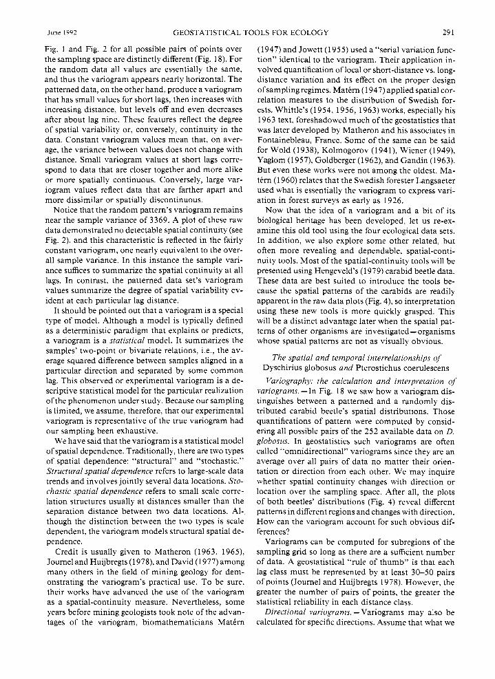
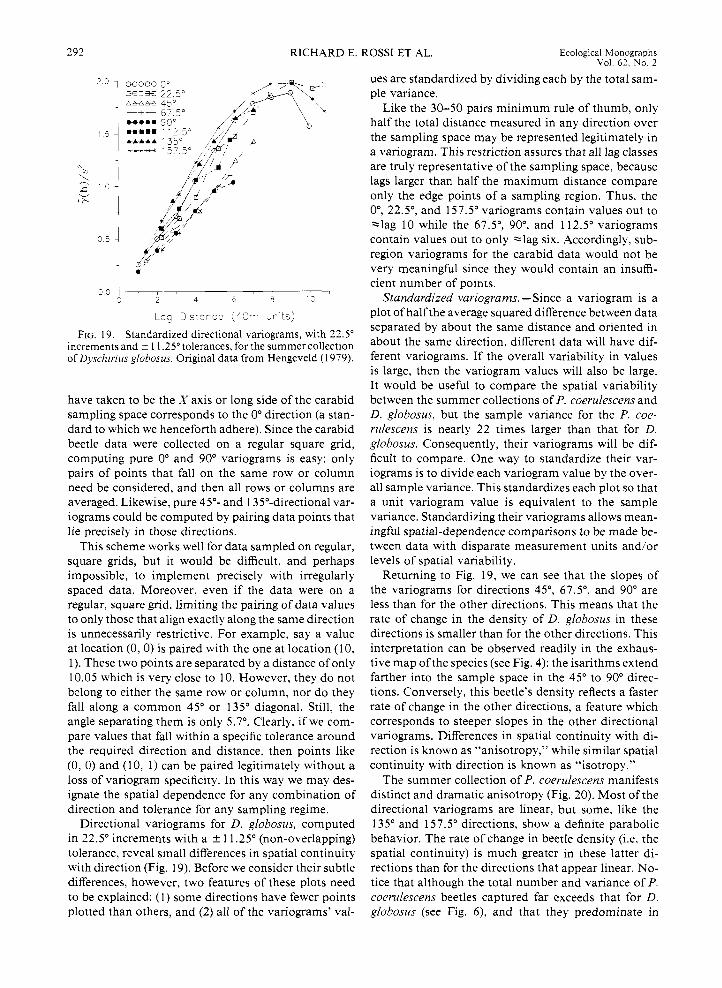
FIG. 19. Standardized directional variograms, with 22.5" increments and ? 1 1.25" tolerances. for the summer collection of Dyschirius globosus. Original data from Hengeveld (1 979).
have taken to be the X axis or long side of the carabid sampling space corresponds to the 0" direction (a stan- dard to which we henceforth adhere). Since the carabid beetle data were collected on a regular square grid, computing pure 0" and 90" variograms is easy: only pairs of points that fall on the same row or column need be considered, and then all rows or columns are averaged. Likewise, pure 45"- and 135"-directional var- iograms could be computed by pairing data points that lie precisely in those directions.
This scheme works well for data sampled on regular, square grids, but it would be difficult, and perhaps impossible, to implement precisely with irregularly spaced data. Moreover, even if the data were on a regular, square grid, limiting the pairing of data values to only those that align exactly along the same direction is unnecessarily restrictive. For example, say a value at location (0 , 0) i s paired with the one at location (1 0, 1). These two points are separated by a distance of only 10.05 which is very close to 10. However, they do not bclong to either the same row or column, nor do they fall along a common 45" or 135" diagonal. Still, the angle separating them is only 5.7". Clearly, if we com- pare values that fall within a specific tolerance around the required direction and distance, then points like (0 , 0) and (10, 1) can be paired legitimately without a loss of variogram specificity. In this way we may des- ignate the spatial dependence for any combination of direction and tolerance for any sampling regime.
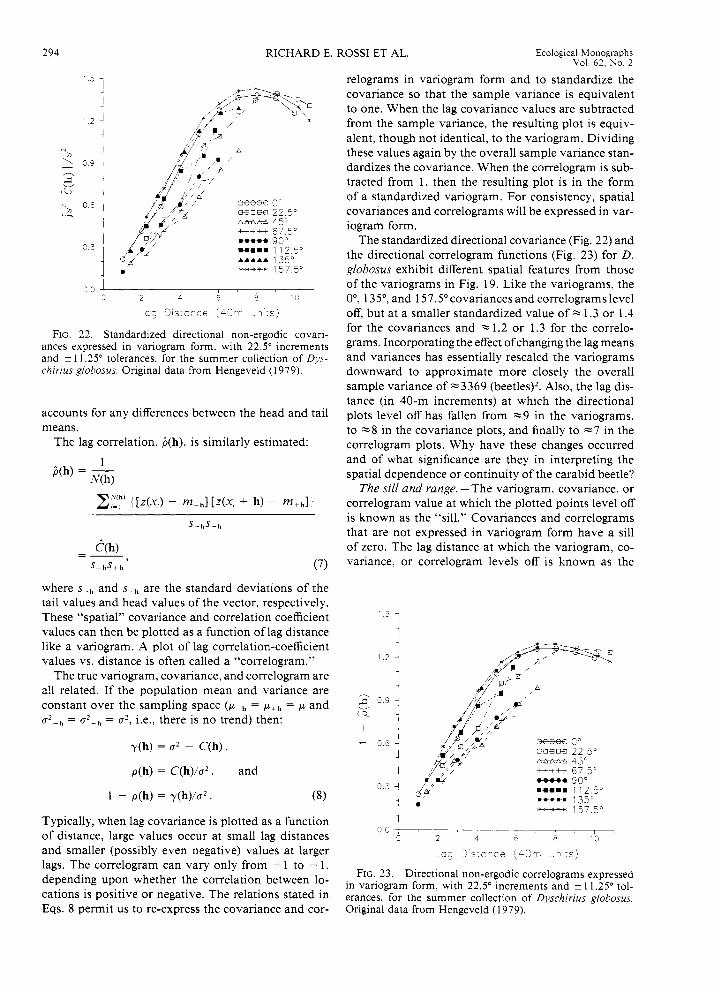
Directional variograms for D. globosus, computed in 22.5" increments with a k 11.25" (non-overlapping) tolerance, reveal small differences in spatial continuity with direction (Fig. 19). Before we consider their subtle differences, however, two features of these plots need to be explained: (1) some directions have fewer points plotted than others, and (2) all of the variograms' val-
ues are standardized by dividing each by the total sam- ple variance.
Like the 30-50 pairs minimum rule of thumb, only half the total distance measured in any direction over the sampling space may be represented legitimately in a variogram. This restriction assures that all lag classes are truly representative of the sampling space, because lags larger than half the maximum distance compare only the edge points of a sampling region. Thus, the O", 22.5", and 157.5" variograms contain values out to "lag 10 while the 67.5", 90°, and 112.5" variograms contain values out to only -lag six. Accordingly, sub- region variograms for the carabid data would not be very meaningful since they would contain an insuffi- cient number of points.
Standardized variograms. -Since a variogram is a plot of half the average squared difference between data separated by about the same distance and oriented in about the same direction, different data will have dif- ferent variograms. If the overall variability in values is large, then the variogram values will also be large. It would be useful to compare the spatial variability between the summer collections of P. coerulescens and D. globosus, but the sample variance for the P. coe- rulescens is nearly 22 times larger than that for D. globosus. Consequently, their variograms will be dif- ficult to compare. One way to standardize their var- iograms is to divide each variogram value by the over- all sample variance. This standardizes each plot so that a unit variogram value is equivalent to the sample variance. Standardizing their variograms allows mean- ingful spatial-dependence comparisons to be made be- tween data with disparate measurement units and/or levels of spatial variability.
Returning to Fig. 19, we can see that the slopes of the variograms for directions 45", 67.5", and 90" are less than for the other directions. This means that the rate of change in the density of D. globosus in these directions is smaller than for the other directions. This interpretation can be observed readily in the exhaus- tive map ofthe species (see Fig. 4): the isarithms extend farther into the sample space in the 45" to 90" direc- tions. Conversely, this beetle's density reflects a faster rate of change in the other directions, a feature which corresponds to steeper slopes in the other directional variograms. Differences in spatial continuity with di- rection is known as "anisotropy," while similar spatial continuity with direction is known as "isotropy."
The summer collection of P. coerulescens manifests distinct and dramatic anisotropy (Fig. 20). Most of the directional variograms are linear, but some, like the 135" and 157.5" directions, show a definite parabolic behavior. The rate of change in beetle density (i.e, the spatial continuity) is much greater in these latter di- rections than for the directions that appear linear. No- tice that although the total number and variance of P. coerulescens beetles captured far exceeds that for D. globosus (see Fig. 6 ) , and that they predominate in
June 1992 GEOSTATISTICAL TOOLS FOR ECOLOGY 293
different regions of the sampling space, a comparison of their directional variograms shows that the rate of change in spatial continuity between the two carabid beetles is, aside from a few directions, comparable with direction. That is, excepting, for example, the 0" and 90" directions, those directions demonstrating the greatest and smallest change in spatial continuity for one beetle also correspond to those for the other. This could signal an environmental or other influence that is shaping similarly the spatial patterns of these two species, species that are quite dissimilar morphologi- cally (Thiele 1977).
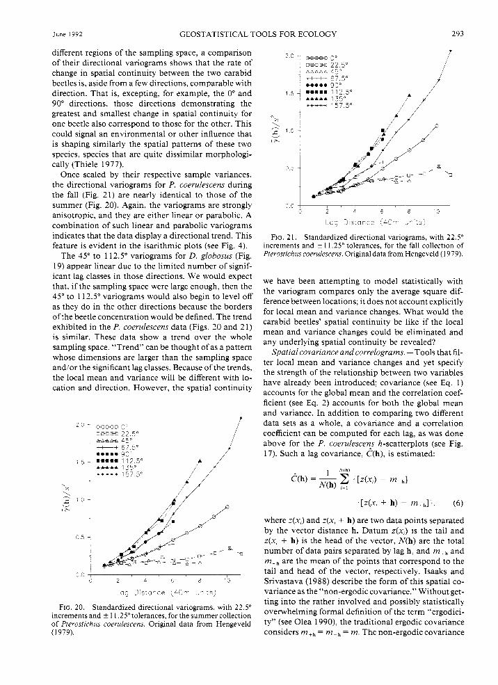
Once scaled by their respective sample variances, the directional variograms for P. coerulescens during the fall (Fig. 21) are nearly identical to those of the summer (Fig. 20). Again, the variograms are strongly anisotropic, and they are either linear or parabolic. A combination of such linear and parabolic variograms indicates that the data display a directional trend. This feature is evident in the isarithmic plots (see Fig. 4).
The 45" to 112.5" variograms for D. globosus (Fig. 19) appear linear due to the limited number of signif- icant lag classes in those directions. We would expect that, if the sampling space were large enough, then the 45" to 1 12.5" variograms would also begin to level off as they do in the other directions because the borders ofthe beetle concentration would be defined. The trend exhibited in the P. coerulescens data (Figs. 20 and 2 1) is similar. These data show a trend over the whole sampling space. "Trend" can be thought of as a pattern whose dimensions are larger than the sampling space and/or the significant lag classes. Because of the trends, the local mean and variance will be different with lo- cation and direction. However, the spatial continuity
N /*/ 1 s l i \
3 0 , ' ' ' , ' , I
0 2 L 5 8 10
-acj ) i s * a i c e ( L O - JI * s )
FIG. 20. Standardized directional variograms, with 22.5" increments and i 1 1.25" tolerances, for the summer collection of Pterostrchus coerulescens Onginal data from Hengeveld (1 979).
N 4
1: g 1 0 -
<Y
0 5 4
0 2 L 8 10 3.0 \ , ,
Lccj 1is:once ( L O T ~ 1 ' : s )
FIG. 21. Standardized directional variograms, with 22.5" increments and i 1 1.25" tolerances, for the fall collection of Pterostichus coerulescens. Original data from Hengeveld (1 979).
we have been attempting to model statistically with the variogram compares only the average square dif- ference between locations; it does not account explicitly for local mean and variance changes. What would the carabid beetles' spatial continuity be like if the local mean and variance changes could be eliminated and any underlying spatial continuity be revealed?
Spatial covariance and correlograms. -Tools that fil- ter local mean and variance changes and yet specify the strength of the relationship between two variables have already been introduced; covariance (see Eq. 1) accounts for the global mean and the correlation coef- ficient (see Eq. 2) accounts for both the global mean and variance. In addition to comparing two different data sets as a whole, a covariance and a correlation coefficient can be computed for each lag, as was done above for the P. coerulescens h-scatterplots (see Fig. 17). Such a lag covariance, C(h), is estimated:
+ h) - m - J } , ( 6 )
where z(x,) and z(x, + h) are two data points separated by the vector distance h. Datum z(x,) is the tail and z(x, + h) is the head of the vector, N(h) are the total number of data pairs separated by lag h, and m-h and m-h are the mean of the points that correspond to the tail and head of the vector, respectively. Isaaks and Srivastava (1 988) describe the form of this spatial co- variance as the "non-ergodic covariance." Without get- ting into the rather involved and possibly statistically overwhelming formal definition of the term "ergodici- ty" (see Olea 1990), the traditional ergodic covariance considers m+h = m-h = m. The non-ergodic covariance
294 RICHARD E. ROSS1 ET AL. Ecological Monographs Vol. 62. No. 2
2 4 e 1 2
Lea ? ' S t C l C E ( 4 2 T J1':S)
FIG. 22. Standardized directional non-ergodic covari- ances expressed in variogram form. with 22.5" increments and i 1 1.25" tolerances, for the summer collection of Dys- chirius globosus. Original data from Hengeveld (1979).
accounts for any differences between the head and tail means.
The lag correlation, fi(h), is similarly estimated:
S-hS+h
(7)
where sxh and s - ~ are the standard deviations of the tail values and head values of the vector, respectively. These "spatial" covariance and correlation coefficient values can then be plotted as a function of lag distance like a variogram. A plot of lag correlation-coefficient values vs. distance is often called a "correlogram."
The true variogram, covariance, and correlogram are all related. If the population mean and variance are constant over the sampling space ( F - ~ = p+h = F and c2_h = c2-h = 02, i.e., there is no trend) then:
y(h) = o2 - C(h),
p(h) = C(h)/c2, and
1 - p(h) = y(h)/02. (8)
Typically, when lag covariance is plotted as a function of distance, large values occur at small lag distances and smaller (possibly even negative) values at larger lags. The correlogram can vary only from + 1 to - 1, depending upon whether the correlation between lo- cations is positive or negative. The relations stated in Eqs. 8 permit us to re-express the covariance and cor-
relograms in variogram form and to standardize the covariance so that the sample variance is equivalent to one. When the lag covariance values are subtracted from the sample variance, the resulting plot is equiv- alent, though not identical, to the variogram. Dividing these values again by the overall sample variance stan- dardizes the covariance. When the correlogram is sub- tracted from 1, then the resulting plot is in the form of a standardized variogram. For consistency, spatial covariances and correlograms will be expressed in var- iogram form.
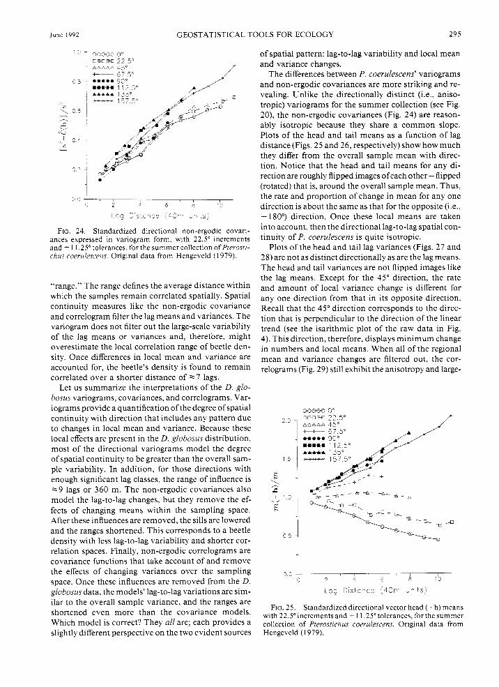
The standardized directional covariance (Fig. 22) and the directional correlogram functions (Fig. 23) for D. globosus exhibit different spatial features from those of the variograms in Fig. 19. Like the variograms, the O", 135", and 157.5" covariances and correlograms level off, but at a smaller standardized value of z 1.3 or 1.4 for the covariances and % 1.2 or 1.3 for the correlo- grams. Incorporating the effect ofchanging the lag means and variances has essentially rescaled the variograms downward to approximate more closely the overall sample variance of ~ 3 3 6 9 (beetles)2. Also, the lag dis- tance (in 40-m increments) at which the directional plots level off has fallen from ~9 in the variograms, to ~8 in the covariance plots, and finally to ~7 in the correlogram plots. Why have these changes occurred and of what significance are they in interpreting the spatial dependence or continuity of the carabid beetle?
The sill and range. -The variogram, covariance, or correlogram value at which the plotted points level off is known as the "sill." Covariances and correlograms that are not expressed in variogram form have a sill of zero. The lag distance at which the variogram, co- variance, or correlogram levels off is known as the
' 5 1
l i l
A
v .c 0 9 4
1 I
I - 0 6 - I
3 3 4
I 0 0 & ' ' ' , ' ' , ' . ^ 4 2 6 8 8J
-09 D ' s t c n c e ( & E r r " l ' t s )
FIG. 23. Directional non-ergodic correlograms expressed in variogram form, with 22.5" increments and i 11.25" tol- erances, for the summer collection of Dyschirius globosus. Original data from Hengeveld (1 979).
June 1992 GEOSTATISTICAL TOOLS FOR ECOLOGY 295
,2 0 , I c 2 I 6 8 13
L c g 3 s :c i ce ( i r -1 ts)
FIG. 24 . Standardized directional non-ergodic covari- ances expressed in variogram form, with 22.5" increments and i 1 1.25" tolerances, for the summer collection of Pterosti- chus coerulescens. Original data from Hengeveld ( 1 979).
"range." The range defines the average distance within which the samples remain correlated spatially. Spatial continuity measures like the non-ergodic covariance and correlogram filter the lag means and variances. The variogram does not filter out the large-scale variability of the lag means or variances and, therefore, might overestimate the local correlation range of beetle den- sity. Once differences in local mean and variance are accounted for, the beetle's density is found to remain correlated over a shorter distance of -7 lags.
Let us summarize the interpretations of the D. glo- bosus variograms, covariances, and correlograms. Var- iograms provide a quantification of the degree of spatial continuity with direction that includes any pattern due to changes in local mean and variance. Because these local effects are present in the D. globosus distribution, most of the directional variograms model the degree of spatial continuity to be greater than the overall sam- ple variability. In addition, for those directions with enough significant lag classes, the range of influence is -9 lags or 360 m. The non-ergodic covariances also model the lag-to-lag changes, but they remove the ef- fects of changing means within the sampling space. After these influences are removed, the sills are lowered and the ranges shortened. This corresponds to a beetle density with less lag-to-lag variability and shorter cor- relation spaces. Finally, non-ergodic correlograms are covariance functions that take account of and remove the effects of changing variances over the sampling space. Once these influences are removed from the D. globosus data, the models' lag-to-lag variations are sim- ilar to the overall sample variance, and the ranges are shortened even more than the covariance models. Which model is correct? They all are; each provides a slightly different perspective on the two evident sources
of spatial pattern: lag-to-lag variability and local mean and variance changes.
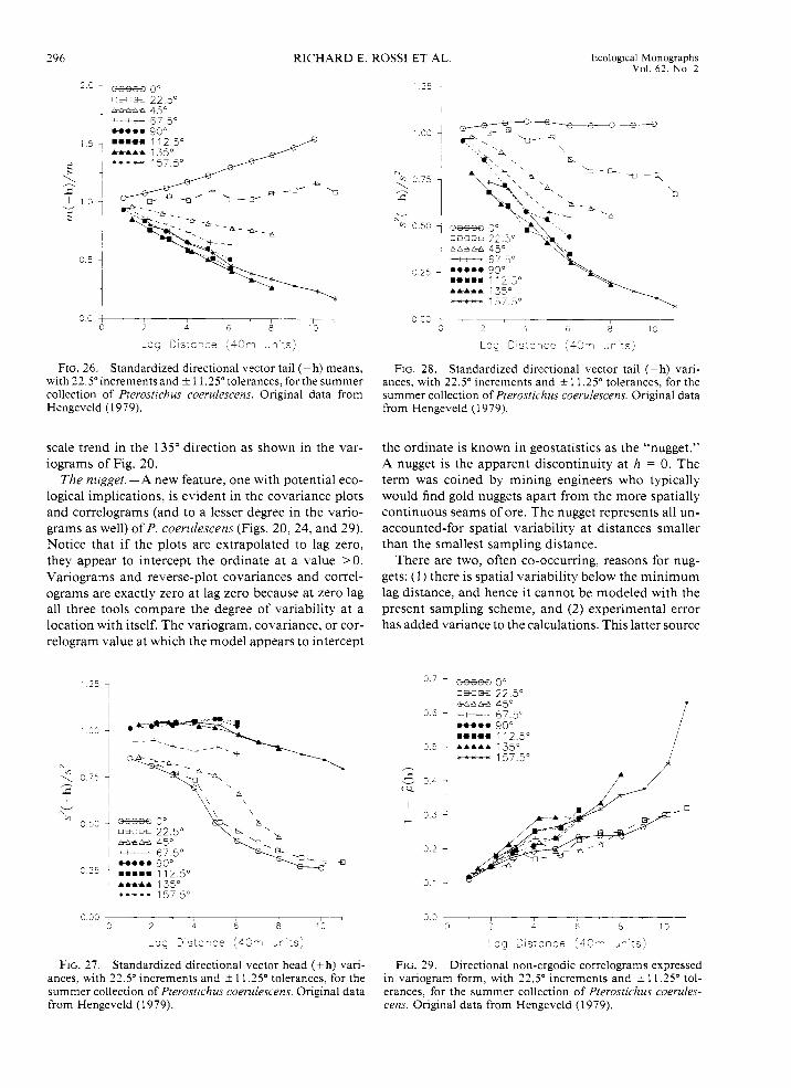
The differences between P. coerulescens' variograms and non-ergodic covariances are more striking and re- vealing. Unlike the directionally distinct (i.e., aniso- tropic) variograms for the summer collection (see Fig. 20), the non-ergodic covariances (Fig. 24) are reason- ably isotropic because they share a common slope. Plots of the head and tail means as a function of lag distance (Figs. 25 and 26, respectively) show how much they differ from the overall sample mean with direc- tion. Notice that the head and tail means for any di- rection are roughly flipped images ofeach other-flipped (rotated) that is, around the overall sample mean. Thus, the rate and proportion of change in mean for any one direction is about the same as that for the opposite (i.e., + 1 80') direction. Once these local means are taken into account, then the directional lag-to-lag spatial con- tinuity of P. coerulescens is quite isotropic.
Plots of the head and tail lag variances (Figs. 27 and 28) are not as distinct directionally as are the lag means. The head and tail variances are not flipped images like the lag means. Except for the 45" direction, the rate and amount of local variance change is different for any one direction from that in its opposite direction. Recall that the 45" direction corresponds to the direc- tion that is perpendicular to the direction of the linear trend (see the isarithmic plot of the raw data in Fig. 4). This direction, therefore, displays minimum change in numbers and local means. When all of the regional mean and variance changes are filtered out, the cor- relograms (Fig. 29) still exhibit the anisotropy and large-
4
G C ~ , ' 1 - C 2 4 6 6 10
L G ~ D is tcnce (4Cr r ~n ts)
FIG. 25 . Standardized directional vector head (+ h) means with 22.5"increments and * 11.25" tolerances, for the summer collection of Pterostichus coerulescens. Original data from Hengeveld ( 1 979).
296 RICHARD E. ROSS1 ET AL. Ecological Monographs Vol. 62. No. 2
-35 U i s t c r c e ( 4 C n ui ' :s)
FIG. 26. Standardized directional vector tail (-h) means, with 22.5"increments and * 1 1.25" tolerances, for the summer collection of Pterostichus coerulescens. Original data from Hengeveld (1 979).
scale trend in the 135" direction as shown in the var- iograms of Fig. 20.
T h e nugget. -A new feature, one with potential eco- logical implications, is evident in the covariance plots and correlograms (and to a lesser degree in the vario- grams as well) of P. coerulescens (Figs. 20, 24, and 29). Notice that if the plots are extrapolated to lag zero, they appear to intercept the ordinate at a value > O . Variograms and reverse-plot covariances and correl- ograms are exactly zero at lag zero because at zero lag all three tools compare the degree of variability at a location with itself. The variogram, covariance, or cor- relogram value at which the model appears to intercept
' 25
. nn Y Y
h 2 075
* 053
c * v h
3 25
FIG. 27. Standardized directional vector head (+h) vari- ances, with 22.5" increments and i 11.25" tolerances, for the summer collection of Pterostichus coerulescens. Original data from Hengeveld (1979).
0 25
0 c 3 ~
2 4 0 8 1 C
LOG U;s:c ice (4,311 ,?ts)
FIG. 28. Standardized directional vector tail (-h) vari- ances, with 22.5" increments and i 11.25" tolerances, for the summer collection of Pterostichus coerulescens. Original data from Hengeveld (1979).
the ordinate is known in geostatistics as the "nugget." A nugget is the apparent discontinuity at h = 0. The term was coined by mining engineers who typically would find gold nuggets apart from the more spatially continuous seams of ore. The nugget represents all un- accounted-for spatial variability at distances smaller than the smallest sampling distance.
There are two, often co-occurring, reasons for nug- gets: (1) there is spatial variability below the minimum lag distance, and hence it cannot be modeled with the present sampling scheme, and ( 2 ) experimental error has added variance to the calculations. This latter source
07
O E
0 5 - - * v 0.4 ( Q
I 0 3 - 0 2
0'
0 3
FIG. 29. Directional non-ergodic correlograms expressed in variogram form, with 22.5" increments and i 11.25" tol- erances, for the summer collection of Pterostichus coerules- cens. Original data from Hengeveld (1979).
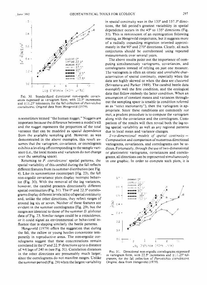
June 1992
c -
1 0 8 1
3.2 4
0 0 1
FIG. 30.
GEOSTATISTICAL TOOLS FOR ECOLOGY 297
f
1 ' 8 c 5 e '0
8 ,
2
!Lag D ' s t a n c e ( L C r J l ' t S )
Standardized directional non-ergodic covari- ances expressed in variogram form, with 22.5" increments and k 11.25" tolerances, for the fall collection of Pterostichus coerulescens. Original data from Hengeveld ( 1 979).
is sometimes termed "the human nugget." Nuggets are important because the difference between a model's sill and the nugget represents the proportion of the total variance that can be modeled as spatial dependence from the available sampling grid. However, as was demonstrated in the above examples, this result as- sumes that the variogram, covariance, or correlogram exhibits a leveling offcorresponding to the sample vari- ance (i.e., the local means and variances do not change over the sampling space).
Returning to P. coerulescens' spatial patterns, the spatial variability of this carabid during the fall reflects different features from its summer distribution (see Fig. 4). Like its summertime counterpart (Fig. 23), the fall non-ergodic covariance plots display isotropic behav- ior (Fig. 30). With the removal of the lag variances, however, the carabid presents directionally different spatial continuities (Fig. 3 1). The 0" and 22.5" correlo- grams display different levels (sills) of spatial continuity and, unlike the other directions, they reflect ranges of around lag six or seven. Neither of these features are evident in the summer correlograms (Fig. 29), but the ranges are identical to those of the summer D. globosus data of Fig. 23. Similar ranges could be a coincidence, or it could signal an environmental or behavioral in- fluence that is shaping similarly the beetle patterns.
Hengeveld (1979) offers the suggestion that during the fall, the callow or young beetles concentrate tem- porarily in reproductive areas. The non-ergodic cor- relograms suggest that these concentrations remain correlated in the 0" and 22.5" directions up to a distance of -6 lags of 240 m (see Fig. 3 1). Correlation distances in the other directions are presumably much larger, since the correlograms do not manifest ranges. Unlike the summer period (Fig. 29) when the largest variability
in spatial continuity was in the 135" and 157.5" direc- tions, the fall period's greatest variability in spatial dependence occurs in the 45" to 135" directions (Fig. 3 1). This is reminiscent of an outmigration following mating, as Hengeveld conjectures, but it suggests more of a radially expanding migration oriented approxi- mately in the 90" and 270" directions. Clearly, all such conjectures should be corroborated using repeated measurements over several years.
The above results point out the importance of com- puting simultaneously variograms, covariances, and correlograms instead of relying on just one measure. The variogram is often an erratic and unreliable char- acterization of spatial continuity, especially when the data are highly skewed or when the data are clustered (Srivastava and Parker 1989). The carabid beetle data exemplify well the first condition, and the ecological data that follow embody the latter condition. When an assumption of constant means and variances through- out the sampling space is tenable (a condition referred as as "strict stationarity"), then the variogram is ap- propriate. Since these conditions are commonly not met, a prudent procedure is to compute the variogram along with the covariance and the correlogram. Com- parison of the results will then reveal both the lag-to- lag spatial variability as well as any regional patterns due to local mean and variance changes.
Two-dimensional models of spatial continuity.- Computation and comparison of numerous directional variograms, covariances, and correlograms can be te- dious. Fortunately, through the use of two-dimensional or planimetric variograms, covariances and correlo- grams, all directions can be represented simultaneously in one graphic. In order to compute such plots, it is
0: -
0 5 c 6 I
- 0 3 .
c ' 2 0.1 1
- A v 0 4 -
' Q
, 4 2 2 6 6 . ^ 0 0 i , ,
-39 I i s i c n c e (4l:r- ~-1'~s)
FIG. 3 1. Directional non-ergodic correlograms expressed in variogram form, with 22.5" increments and * 11.25" tol- erances, for the fall collection of Pterostichus coerulescens. Original data from Hengeveld (1979).
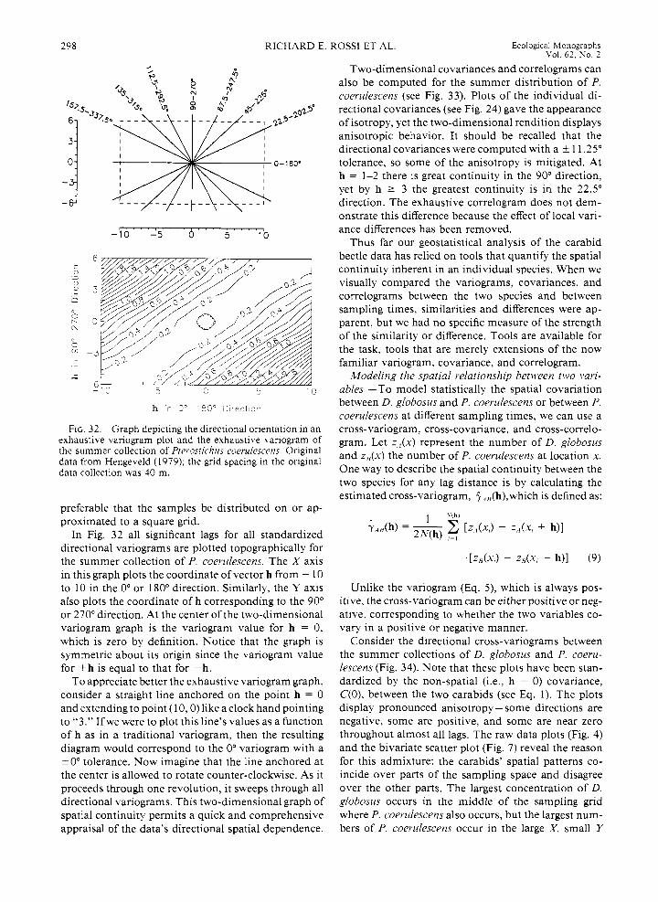
298 RICHARD E. ROSS1 ET AL. Ecological Monographs Val. 62. No. 2
, , Two-dimensional covariances and correlograms can also be computed for the summer distribution of P. coerulescens (see Fig. 33). Plots of the individual di- rectional covariances (see Fig. 24) gave the appearance of isotropy, yet the two-dimensional rendition displays anisotropic behavior. It should be recalled that the directional covariances were computed with a i 1 1.25" tolerance, so some of the anisotropy is mitigated. At h = 1-2 there is great continuity in the 90" direction, yet by h 2 3 the greatest continuity is in the 22.5" direction. The exhaustive correlogram does not dem- onstrate this difference because the effect of local vari-
Thus far our geostatistical analysis of the carabid beetle data has relied on tools that quantify the spatial
_202.5e
r . I , , I . I I - . . , . . . . , ance differences has been removed. -10 1 5 0 5 10
6 C
. _ 0 continuity inherent in an individual species. When we visually compared the variograms, covariances, and i
r'
3 correlograms between the two species and between sampling times, similarities and differences were ap- parent, but we had no specific measure of the strength
the task, tools that are merely extensions of the now
. - , Y 3
b r . 3 N
3 - 3 .- C
1 I
I
0 of the similarity or difference. Tools are available for
familiar variogram, covariance, and correlogram. Modeling the spatial relationship between two vari-
- 1 : -5 " 5 I c ables. -To model statistically the spatial covariation between D. globosus and P. coerulescens or between P. coerulescens at different sampling times, we can use a cross-variogram, cross-covariance, and cross-correlo- gram, Let zi(x) represent the number of D, globosus and zg(x) the number of p , coerulescens at location x, One way to describe the spatial continuity between the two species for any lag distance is by calculating the estimated cross-variogram, +,,(h),which is defined as:
? - D
h in C0-183O Direc t lo?
FIG. 32. Graph depicting the directional orientation in an exhaustive vanogram plot and the exhaustive variogram Of the summer collection of Ptcrostichus coerulescens. Original data from Hengeveld ( 1 979); the grid spacing in the original data collection was 40 m.
preferable that the samples be distributed on or ap- proximated to a square grid.
In Fig. 32 all significant lags for all standardized directional variograms are plotted topographically for the summer collection of P. coerulescens. The X axis in this graph plots the coordinate of vector h from - 10 to 10 in the 0" or 180" direction. Similarly, the Y axis also plots the coordinate of h corresponding to the 90" or 270" direction. At the center of the two-dimensional variogram graph is the variogram value for h = 0, which is zero by definition. Notice that the graph is symmetric about its origin since the variogram value for + h is equal to that for - h.
To appreciate better the exhaustive variogram graph, consider a straight line anchored on the point h = 0 and extending to point (1 0,O) like a clock hand pointing to "3." Ifwe were to plot this line's values as a function of h as in a traditional variogram, then the resulting diagram would correspond to the 0" variogram with a i0" tolerance. Now imagine that the line anchored at the center is allowed to rotate counter-clockwise. As it proceeds through one revolution, it sweeps through all directional variograms. This two-dimensional graph of spatial continuity permits a quick and comprehensive appraisal of the data's directional spatial dependence.
1 \ ( h )
+ A h ) = - 2 [z,(x,) - z.i(x, + h)l 2h(h) ,=,
"z,(x,) - Zi3(Xi + h)l (9)
Unlike the variogram (Eq. 5 ) , which is always pos- itive, the cross-variogram can be either positive or neg- ative, corresponding to whether the two variables co- vary in a positive or negative manner.
Consider the directional cross-variograms between the summer collections of D. globosus and P. coeru- lescens (Fig. 34). Note that these plots have been stan- dardized by the non-spatial (i.e., h = 0) covariance, C(O), between the two carabids (see Eq. 1). The plots display pronounced anisotropy- some directions are negative, some are positive, and some are near zero throughout almost all lags. The raw data plots (Fig. 4) and the bivariate scatter plot (Fig. 7) reveal the reason for this admixture: the carabids' spatial patterns co- incide over parts of the sampling space and disagree over the other parts. The largest concentration of D. globosus occurs in the middle of the sampling grid where P. coerulescens also occurs, but the largest num- bers of P. coerulescens occur in the large X, small Y
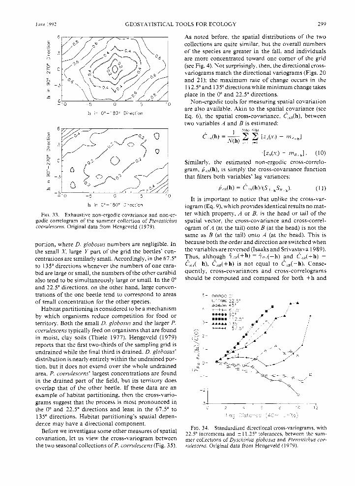
June 1992 GEOSTATISTICAL TOOLS FOR ECOLOGY 299
c -
h in 0"-1 90" Direct'on
h in 0"-1 90" Direct'on
FIG. 33. Exhaustive non-ergodic covariance and non-er- godic correlogram of the summer collection of Pterostichus coerulescens. Original data from Hengeveld ( 1 979).
portion, where D. globosus numbers are negligible. In the small X , large Y part of the grid the beetles' con- centrations are similarly small. Accordingly, in the 67.5" to 135" directions whenever the numbers of one cara- bid are large or small, the numbers of the other carabid also tend to be simultaneously large or small. In the 0" and 22.5" directions, on the other hand, large concen- trations of the one beetle tend to correspond to areas of small concentration for the other species.
Habitat partitioning is considered to be a mechanism by which organisms reduce competition for food or territory. Both the small D. globosus and the larger P. coerulescens typically feed on organisms that are found in moist, clay soils (Thiele 1977). Hengeveld ( 1 979) reports that the first two-thirds of the sampling grid is undrained while the final third is drained. D. globosus' distribution is nearly entirely within the undrained por- tion, but it does not extend over the whole undrained area. P. coerulescens' largest concentrations are found in the drained part of the field, but its territory does overlap that of the other beetle. If these data are an example of habitat partitioning, then the cross-vario- grams suggest that the process is most pronounced in the 0" and 22.5" directions and least in the 67.5" to 135" directions. Habitat partitioning's spatial depen- dence may have a directional component.
Before we investigate some other measures of spatial covariation, let us view the cross-variogram between the two seasonal collections o f P . coerulescens (Fig. 35).
As noted before, the spatial distributions of the two collections are quite similar, but the overall numbers of the species are greater in the fall, and individuals are more concentrated toward one comer of the grid (see Fig. 4). Not surprisingly, then, the directional cross- variograms match the directional variograms (Figs. 20 and 21); the maximum rate o f change occurs in the 1 12.5" and 135" directions while minimum change takes place in the 0" and 22.5" directions.
Non-ergodic tools for measuring spatial covariation are also available. Akin to the spatial covariance (see Eq. 6), the spatial cross-covariance, C,,(h), between two variables A and B is estimated:
' [ z ! j ( x ) ) - m / j + h l ' ( lo) Similarly, the estimated non-ergodic cross-correlo- gram, ,b ,B(h), is simply the cross-covariance function that filters both variables' lag variances:
dl,(h) = ~18(h)Y(sl-hsB-h). ( 1 1)
It is important to notice that unlike the cross-var- iogram (Eq. 9), which provides identical results no mat- ter which property, A or B, is the head or tail of the spatial vector, the cross-covariance and cross-correl- ogram of A (at the tail) onto B (at the head) is not the same as B (at the tail) onto A (at the head). This is because both the order and direction are switched when the variables are reversed (Isaaks and Srivastava 1989). Thus, although ? I B ( + ~ ) = ?m(-h) and C,,(+h) =
eB4(-h) , d,,lB(+h) is not equal to &(-h). Conse- quently, cross-covariances and cross-correlograms should be computed and compared for both S h and
FIG. 34. Standardized directional cross-variograms. with 22.5" increments and T 11.25" tolerances, between the sum- mer collections of Dvschirius globosus and Pterostichus coe- rulescens. Original data from Hengeveld ( 1 979).
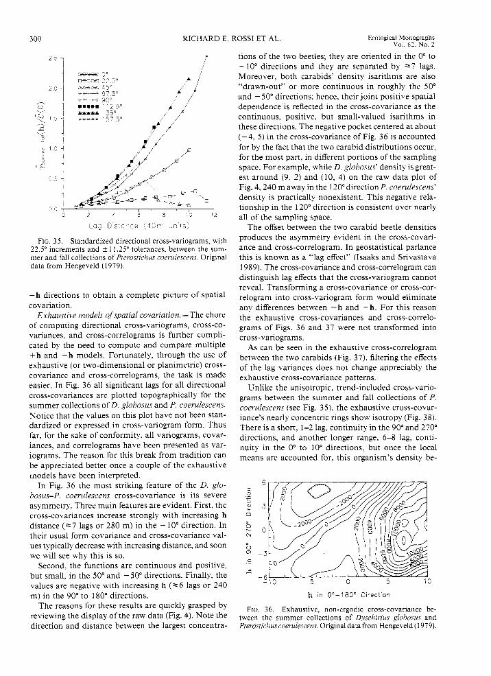
RICHARD E. ROSS1 ET AL. Ecological Monographs Vol. 62. No. 2
*
L O ? D i s t c - c e :40rr -;.'ts:
FIG. 35. Standardized directional cross-variograms, with 22.5" increments and * 11.25" tolerances. between the sum- mer and fall collections of Pterostichus coerulescens. Original data from Hengeveld ( 1 979).
-h directions to obtain a complete picture of spatial covariation.
Exhaustive models of spatial covariation. - The chore of computing directional cross-variograms, cross-co- variances, and cross-correlograms is further compli- cated by the need to compute and compare multiple + h and - h models. Fortunately, through the use of exhaustive (or two-dimensional or planimetric) cross- covariance and cross-correlograms, the task is made easier. In Fig. 36 all significant lags for all directional cross-covariances are plotted topographically for the summer collections of D. globosus and P. coerulescens. Notice that the values on this plot have not been stan- dardized or expressed in cross-variogram form. Thus far, for the sake of conformity, all variograms, covar- iances, and correlograms have been presented as var- iograms. The reason for this break from tradition can be appreciated better once a couple of the exhaustive models have been interpreted.
In Fig. 36 the most striking feature of the D. glo- bosus-P. coerulescens cross-covariance is its severe asymmetry. Three main features are evident. First, the cross-covariances increase strongly with increasing h distance (2 7 lags or 280 m) in the - 10" direction. In their usual form covariance and cross-covariance val- ues typically decrease with increasing distance, and soon we will see why this is so.
Second, the functions are continuous and positive, but small, in the 50" and - 50" directions. Finally, the values are negative with increasing h (-6 lags or 240 m) in the 90" to 180" directions.
The reasons for these results are quickly grasped by reviewing the display of the raw data (Fig. 4). Note the direction and distance between the largest concentra-
tions of the two beetles; they are oriented in the 0" to - 10" directions and they are separated by =7 lags. Moreover, both carabids' density isarithms are also "drawn-out'' or more continuous in roughly the 50" and - 50" directions; hence, their joint positive spatial dependence is reflected in the cross-covariance as the continuous, positive, but small-valued isarithms in these directions. The negative pocket centered at about (-4, 5) in the cross-covariance of Fig. 36 is accounted for by the fact that the two carabid distributions occur, for the most part, in different portions of the sampling space. For example, while D. globosus' density is great- est around (9, 2) and ( lo , 4) on the raw data plot of Fig. 4,240 m away in the 120" direction P. coerulescens' density is practically nonexistent. This negative rela- tionship in the 120" direction is consistent over nearly all of the sampling space.
The offset between the two carabid beetle densities produces the asymmetry evident in the cross-covari- ance and cross-correlogram. In geostatistical parlance this is known as a "lag effect" (Isaaks and Srivastava 1989). The cross-covariance and cross-correlogram can distinguish lag effects that the cross-variogram cannot reveal. Transforming a cross-covariance or cross-cor- relogram into cross-variogram form would eliminate any differences between + h and - h. For this reason the exhaustive cross-covariances and cross-correlo- grams of Figs. 36 and 37 were not transformed into cross-variograms.
As can be seen in the exhaustive cross-correlogram between the two carabids (Fig. 37), filtering the effects of the lag variances does not change appreciably the exhaustive cross-covariance patterns.
Unlike the anisotropic, trend-included cross-vario- grams between the summer and fall collections of P. coerulescens (see Fig. 3 5), the exhaustive cross-covar- iance's nearly concentric rings show isotropy (Fig. 38). There is a short, 1-2 lag, continuity in the 90" and 270" directions, and another longer range, 6-8 lag, conti- nuity in the 0" to 10" directions, but once the local means are accounted for, this organism's density be-
6 C 0
0 ._ c
. _ Y 3 0
0
N I 0
r . 0
-3 C .- c
-10 -5 0 5 10 -6
h in 0"-180" Direction
FIG. 36. Exhaustive, non-ergodic cross-covariance be- tween the summer collections of Dyschirius globosus and Pterostichus coerulescens. Original data from Hengeveld (1 979).
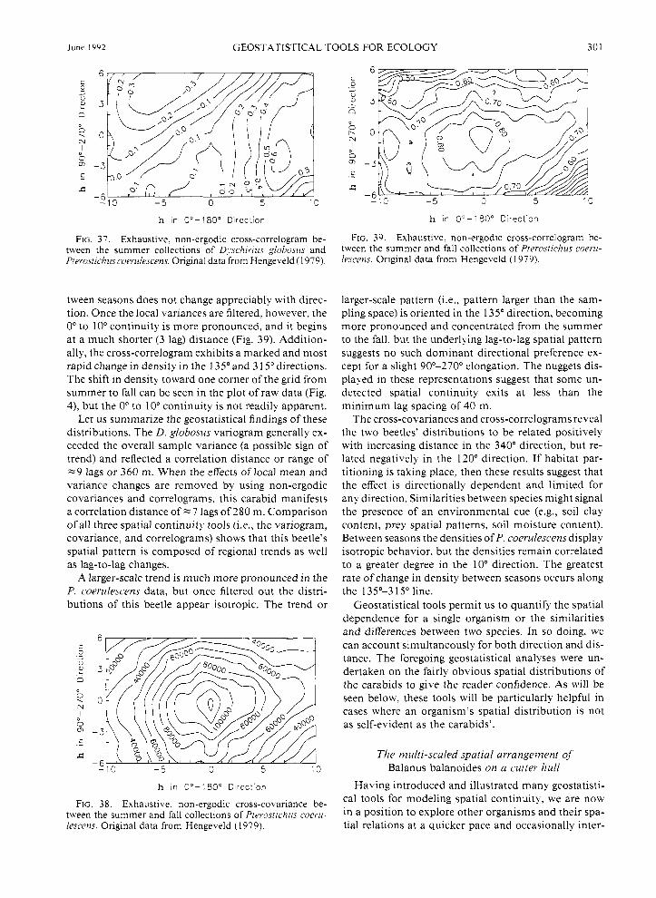
June 1992 GEOSTATISTICAL TOOLS FOR ECOLOGY 30 1
6 c 0
0
. _ +-
.- ? 3
b 0
r . 0
C
-10 -5 5 10 0
N I 0
-3 . - s
-6
h in 0"-190" Direction
FIG. 37. Exhaustive. non-ergodic cross-correlogram be- tween the summer collections of D1schiriu.s globosus and Pterostrchtiscoerirlescens. Ongmal data from Hengeveld (1 979).
tween seasons does not change appreciably with direc- tion. Once the local variances are filtered, however, the 0" to 10" continuity is more pronounced, and it begins at a much shorter (3 lag) distance (Fig. 39). Addition- ally, the cross-correlogram exhibits a marked and most rapid change in density in the 135" and 3 15" directions. The shift in density toward one corner of the grid from summer to fall can be seen in the plot of raw data (Fig. 4), but the 0" to 10" continuity is not readily apparent.
Let us summarize the geostatistical findings of these distributions. The D. globosus variogram generally ex- ceeded the overall sample variance (a possible sign of trend) and reflected a correlation distance or range of x 9 lags or 360 m. When the effects of local mean and variance changes are removed by using non-ergodic covariances and correlograms, this carabid manifests a correlation distance of 7 lags of 280 m. Comparison of all three spatial continuity tools (i.e., the variogram, covariance, and correlograms) shows that this beetle's spatial pattern is composed of regional trends as well as lag-to-lag changes.
A larger-scale trend is much more pronounced in the P. coerulescens data, but once filtered out the distri- butions of this beetle appear isotropic. The trend or
0 m C .- s
6
3
0
-3
-10 -5 0 5 10 -6
6 C 0
0 .- c
. _ ? 3 n ?2 r . 0 N
I 0
C -3
.- c
-10 -5 0 5 10 -6
h in 0"-150" Direct'on
FIG. 39. Exhaustive. non-ergodic cross-correlogram be- tween the summer and fall collections of Pterostichus coeru- lescens. Original data from Hengeveld (1979).
larger-scale pattern (i.e., pattern larger than the sam- pling space) is oriented in the 135" direction, becoming more pronounced and concentrated from the summer to the fall, but the underlying lag-to-lag spatial pattern suggests no such dominant directional preference ex- cept for a slight 90°-2700 elongation. The nuggets dis- played in these representations suggest that some un- detected spatial continuity exits at less than the minimum lag spacing of 40 m.
The cross-covariances and cross-correlograms reveal the two beetles' distributions to be related positively with increasing distance in the 340" direction, but re- lated negatively in the 120" direction. If habitat par- titioning is taking place, then these results suggest that the effect is directionally dependent and limited for any direction. Similarities between species might signal the presence of an environmental cue (e.g., soil clay content, prey spatial patterns, soil moisture content). Between seasons the densities of P. coerulescens display isotropic behavior, but the densities remain correlated to a greater degree in the 10" direction. The greatest rate of change in density between seasons occurs along the 135"-3 15" line.
Geostatistical tools permit us to quantify the spatial dependence for a single organism or the similarities and differences between two species. In so doing, we can account simultaneously for both direction and dis- tance. The foregoing geostatistical analyses were un- dertaken on the fairly obvious spatial distributions of the carabids to give the reader confidence. As will be seen below, these tools will be particularly helpful in cases where an organism's spatial distribution is not as self-evident as the carabids'.
The multi-scaled spatial arrangement of Balanus balanoides on a cutter hull
h in 0"-150" Direct'on Having introduced and illustrated many geostatisti- cal tools for modeling spatial continuity, we are now in a Position to explore other organisms and their spa- tial relations at a quicker pace and occasionally inter-
FIG. 38. Exhaustive, non-ergodic cross-covariance be- tween the summer and fall collections of Pterostjchus coeru- lescens. Original data from Hengeveld (1 979).
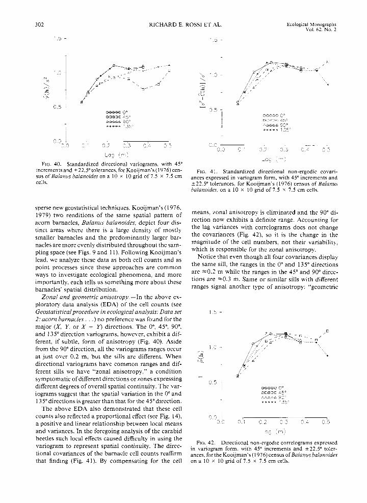
302 RICHARD E. ROSS1 ET AL. Ecological Monographs Vol. 62, No. 2
1.5 -
d
~ a g ( r i )
FIG. 40. Standardized directional variograms, with 45" increments and i22.5" tolerances, for Kooijman's ( 1 976) cen- sus of Balanus balanoides on a 10 x 10 grid of 7.5 x 7.5 cm cells.
sperse new geostatistical techniques. Kooijman's (1 976, 1979) two renditions of the same spatial pattern of acorn barnacles, Balanus balanoides, depict four dis- tinct areas where there is a large density of mostly smaller barnacles and the predominantly larger bar- nacles are more evenly distributed throughout the sam- pling space (see Figs. 9 and 11). Following Kooijman's lead, we analyze these data as both cell counts and as point processes since these approaches are common ways to investigate ecological phenomena, and more importantly, each tells us something more about these barnacles' spatial distribution.
Zonal and geometric anisotropy. -In the above ex- ploratory data analysis (EDA) of the cell counts (see Geostatisticalprocedure in ecological analysis: Data set 2: acorn barnacles . . .) no preference was found for the major (X, Y, or X + Y) directions. The O", 45", 90", and 135" direction variograms, however, exhibit a dif- ferent, if subtle, form of anisotropy (Fig. 40). Aside from the 90" direction, all the variograms ranges occur at just over 0.2 m, but the sills are different. When directional variograms have common ranges and dif- ferent sills we have "zonal anisotropy," a condition symptomatic of different directions or zones expressing different degrees of overall spatial continuity. The var- iograms suggest that the spatial variation in the 0" and 135" directions is greater than that for the 45" direction.
The above EDA also demonstrated that these cell counts also reflected a proportional effect (see Fig. 14), a positive and linear relationship between local means and variances. In the foregoing analysis of the carabid beetles such local effects caused difficulty in using the variogram to represent spatial continuity. The direc- tional covariances of the barnacle cell counts reaffirm that finding (Fig. 41). By compensating for the cell
3.3 r, r 3.0 z ' z . 2 z . 3 3 . 1 "
# \ -c; ,n,
FIG. 4 1. Standardized directional non-ergodic covari- ances expressed in variogram form, with 45" increments and i22.5" tolerances, for Kooijman's (1976) census of Balanus balanoides, on a 10 x 10 grid of 7.5 x 7.5 cm cells.
means, zonal anisotropy is eliminated and the 90" di- rection now exhibits a definite range. Accounting for the lag variances with correlograms does not change the covariances (Fig. 42), so it is the change in the magnitude of the cell numbers, not their variability, which is responsible for the zonal anisotropy.
Notice that even though all four covariances display the same sill, the ranges in the 0" and 135" directions are e0 .2 m while the ranges in the 45" and 90" direc- tions are e 0 . 3 m. Same or similar sills with different ranges signal another type of anisotropy: "geometric
1.3 4
7
Q.5 i
0.0 + 0.':
FIG. 42. Directional non-ergodic correlograms expressed in variogram form, with 45" increments and k22.5" toler- ances, for the Kooijman's (1 976) census of Balanus balanoides on a 10 x 10 grid of 7.5 x 7.5 cm cells.
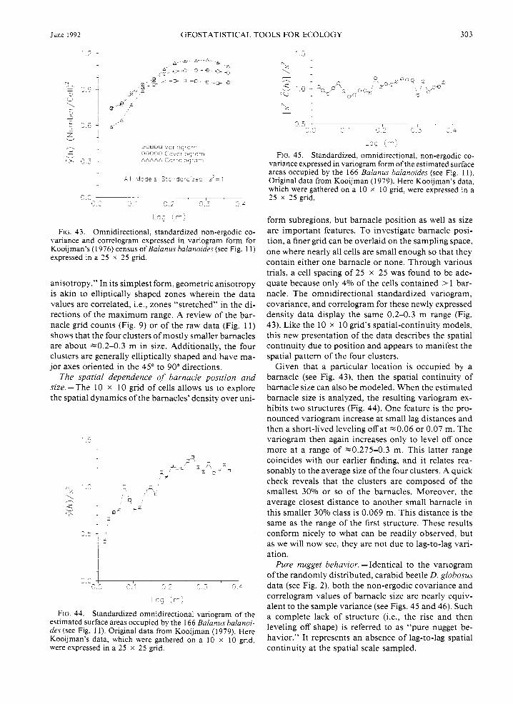
June 1992 GEOSTATISTICAL TOOLS FOR ECOLOGY 303
FIG. 43. Omnidirectional, standardized non-ergodic co- variance and correlogram expressed in variogram form for Kooijman’s ( 1 976) census of Balanus halanoides (see Fig. 1 1 ) expressed in a 25 x 2 5 grid.
anisotropy.” In its simplest form, geometric anisotropy is akin to elliptically shaped zones wherein the data values are correlated, i.e., zones “stretched” in the di- rections of the maximum range. A review of the bar- nacle grid counts (Fig. 9) or of the raw data (Fig. 1 1 ) shows that the four clusters of mostly smaller barnacles are about ~ 0 . 2 - 0 . 3 m in size. Additionally, the four clusters are generally elliptically shaped and have ma- jor axes oriented in the 45” to 90” directions.
The spatial dependence of barnacle position and size. -The 10 x 10 grid of cells allows us to explore the spatial dynamics of the barnacles’ density over uni-
15
FIG. 44. Standardized omnidirectional variogram of the estimated surface areas occupied by the 166 Balanus balanoi- des (see Fig. 1 1). Original data from Kooijman (1979). Here Kooijman’s data, which were gathered on a 10 x 10 grid, were expressed in a 25 x 25 grid.
r - “ 3 , ‘I -... 8- 8- ’ 8- - . L - ‘2 3 ^ 4
-34 ( - 1 ;
FIG. 45. Standardized, omnidirectional, non-ergodic co- variance expressed in variogram form of the estimated surface areas occupied by the 166 Balanus balanoides (see Fig. 11) . Original data from Kooijman (1979). Here Kooijman’s data, which were gathered on a 10 x 10 grid, were expressed in a 25 x 25 grid.
form subregions, but barnacle position as well as size are important features. To investigate barnacle posi- tion, a finer grid can be overlaid on the sampling space, one where nearly all cells are small enough so that they contain either one barnacle or none. Through various trials, a cell spacing of 25 x 25 was found to be ade- quate because only 4% of the cells contained > 1 bar- nacle. The omnidirectional standardized variogram, covariance, and correlogram for these newly expressed density data display the same 0.2-0.3 m range (Fig. 43). Like the 10 x 10 grid’s spatial-continuity models, this new presentation of the data describes the spatial continuity due to position and appears to manifest the spatial pattern of the four clusters.
Given that a particular location is occupied by a barnacle (see Fig. 43), then the spatial continuity of barnacle size can also be modeled. When the estimated barnacle size is analyzed, the resulting variogram ex- hibits two structures (Fig. 44). One feature is the pro- nounced variogram increase at small lag distances and then a short-lived leveling off at ~ 0 . 0 6 or 0.07 m. The variogram then again increases only to level off once more at a range of ~0.275-0.3 m. This latter range coincides with our earlier finding, and it relates rea- sonably to the average size of the four clusters. A quick check reveals that the clusters are composed of the smallest 30% or so of the barnacles. Moreover, the average closest distance to another small barnacle in this smaller 30% class is 0.069 m. This distance is the same as the range of the first structure. These results conform nicely to what can be readily observed, but as we will now see, they are not due to lag-to-lag vari- ation.
Pure nugget behavzor. -Identical to the vanogram of the randomly distributed, carabid beetle D. globosus data (see Fig. 2), both the non-ergodic covariance and correlogram values of barnacle size are nearly equiv- alent to the sample variance (see Figs. 45 and 46). Such a complete lack of structure (i.e., the rise and then leveling off shape) is referred to as “pure nugget be- havior.” It represents an absence of lag-to-lag spatial continuity at the spatial scale sampled.
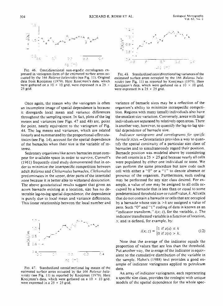
304
1 5 -
RICHARD E. ROSS1 ET AL. Ecological Monographs Vol. 6 2 , No. 2
3 4 - 7 - 1 u L ^ ^ ” ”
- 5 _I
3 g - FIG 46 Omnidirectional non-ergodic correlogram ex-
pressed in vanogram form of the estimated surface areas oc- cupied by the 166 Balanus balanoides (see Fig 1 1 ) Original data from Kooijman (1979) Here Kooijman’s data, which were gathered on a 10 x 10 grid. were expressed in a 25 X
25 grid
FIG. 48. Standardized omnidirectional lag variances ofthe estimated surface areas occupied by the 166 Balanus bala- noides (see Fig. 1 1 ) as reported by Kooijman (1979). Here Kooijman’s data, which were gathered on a 10 x 10 grid, were expressed in a 25 x 25 grid.
Once again, the reason why the variogram is often an incomplete image of spatial dependence is because it disregards local mean and variance differences throughout the sampling space. In fact, plots of the lag means and variances (see Figs. 47 and 48) are, point for point, nearly equivalent to the variogram of Fig. 44. The lag means and variances, which are related linearly and summarized by the proportional-effect sta- tistics (see Fig. 14), account for the spatial dependence of the barnacles when their size is the variable of in- terest.
Sedentary organisms like acorn barnacles must com- Pete for available space in order to survive. Connell’s (1 96 1) frequently cited study demonstrated that in or- der to minimize the interspecific competition between adult Balanus and Chthamalus barnacles, Chthamalus predominates in the upper, drier parts of the intertidal zone because it is better able to withstand desiccation. The above geostatistical results suggest that given an acorn barnacle existing at a location, size has no de- tectable lag-to-lag spatial dependence; the dependence is purely due to local mean and variance differences. This linear relationship between the local number and
variance of barnacle sizes may be a reflection of the organism’s ability to minimize intraspecific competi- tion. Regions with many (small) individuals also have the smallest size variation. Conversely, areas with large individuals are separated by relatively open areas. There is another way, however, to quantify the lag-to-lag spa- tial dependence of barnacle size.
Indicator variograms and correlograms for specific barnacle sizes. -Geostatistics provides a way to quan- tify the spatial continuity of a particular size class of barnacles and to simultaneously regard their position. Barnacle position was modeled above by considering the cell counts in a 25 x 25 grid because nearly all cells were populated by either one individual or none. We can perform the same procedure but now code each cell with either a “0” or a “1” to denote absence or presence of the organism. Furthermore, such coding may be performed for any size class desired. For ex- ample, a value of one may be assigned to all cells oc- cupied by a barnacle that is less than or equal to some predetermined threshold size or cutoff value, k. All cells that do not contain a barnacle or cells that are occupied by a barnacle whose size is > k are assigned a value of zero. Such “0” and “1” coding of data is known as an “indicator transform,” i ( x ; z ) , for the variable, z. The indicator transformed variable is a function of location,
’ 2 - - + + x , and is defined, for example, by:
(12) 1 if z ( x ) 5 k 0 if z ( x ) > k.
,* f , / ‘* **F+ f l k ’ -
i (x ; z ) = 1 2 i
FIG. 47. Standardized omnidirectional lag means of the estimated surface areas occupied by the 166 Balanus bala- noides (see Fig. 1 1 ) as reported by Kooijman (1979). Here Kooijman’s data, which were gathered on a 10 x 10 grid, were expressed in a 25 x 25 grid.
Note that :he average of the indicator equals the proportion of values that are less than the threshold. Put another way, the average of the indicator is equiv- alent to the cumulative distribution of the variable in the sample. Hohn’s (1988) text provides a good ex- ample of indicator variograms applied to petroleum data.
An array of indicator variograms, each representing a specific size class, provides the ecologist with unique models of the spatial dependence for the whole spec-
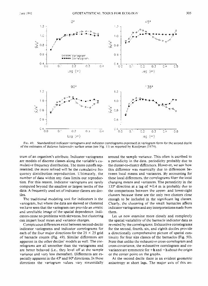
June 1992 GEOSTATISTICAL TOOLS FOR ECOLOGY 305
3" 45" 1.2 1 1.2 1
0.6 1 m e w Variogrom ****a Cor,elogrom i
0.6
0.4 1 0 0 0.1 0.2 0.3 0.4 0.5
0.4 1 0.0 0.1 0.2 0.3 0.4
Log (m) Log (m)
90" 135"
1.2 1
0.6 j i
0.6 1 I
c .4 I 0 4 1 I , , , , , , , I I 0.0 0. 0.2 0.3 0 .L 0.0 0.' 0.2 0.3 0.4 0.5
Log (m) Log (m)
FIG. 49. Standardized indicator variograms and indicator correlograms expressed in variogram form for the second decile of the estimates of Bulunus bulunoides surface areas (see Fig. 1 1 ) as reported by Kooijman (1979).
trum of an organism's attribute. Indicator variograms are models of discrete classes along the variable's cu- mulative frequency distribution. The more cutoffs rep- resented, the more refined will be the cumulative fre- quency distribution reproduction. Ultimately, the number of data within any class limits our reproduc- tion. For this reason, indicator variograms are rarely computed beyond the smallest or largest tenths of the data. A frequently used set of indicator classes are dec- iles.
The traditional modeling tool for indicators is the variogram, but where the data are skewed or clustered we have seen that the variogram can provide an erratic and unreliable image of the spatial dependence. Indi- cators cause no problems with skewness, but clustering can impart local mean and variance changes.
Conspicuous differences exist between second-decile indicator variograms and indicator correlograms for each of the four major directions for the 25 x 25 grid of barnacle counts (Fig. 49). Similar differences are apparent in the other deciles' models as well. The cor- relograms are all smoother than the variograms and are better behaved (i.e., they level off at the sample variance and vary less thereafter). Differences are es- pecially apparent in the 45" and 90" directions. In these directions the variogram values vary sinusoidally
around the sample variance. This often is ascribed to a periodicity in the data, periodicity probably due to the cluster-to-cluster differences. However, we saw how this difference was essentially due to differences be- tween local means and variances. By accounting for these local differences, the correlograms filter the local changing means and variances. The periodicity in the 135" direction at a lag of ~ 0 . 4 m is probably due to the comparisons between the upper- and lower-right clusters because these are the only two clusters close enough to be included in the significant lag classes. Clearly, the clustering of the small barnacles affects indicator variograms and any interpretations made from them.
Let us now examine more closely and completely the spatial variability of the barnacle indicator data as revealed by the correlograms. Exhaustive correlograms for the second, fourth, six, and eighth deciles provide a directionally comprehensive picture of spatial con- tinuity for four size classes of the barnacles (Fig. 50). Note that unlike the exhaustive cross-correlogram and cross-covariance, the exhaustive correlogram and co- variance are symmetric for + h and - h about the origin or the center point on the graphs.
At the second decile there is an evident geometric anisotropy at short lags. The major axis of this an-
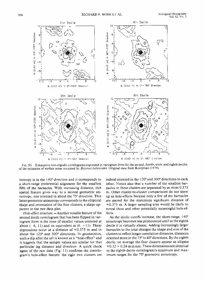
306 Ecological Monographs Vol. 62, No. 2
RICHARD E. ROSS1 ET AL.
21c Decile 4th Decile
- 4 r h (0 03 m) in Oo-180" Direction
6th Decile
-1212 -8 - 4 0 4 8 12
h (0.03 rn) in 0"-180" Direction
8th Decile
h (0.03 rn) in 0"-180' Direction h (0.03 rn) in 0"-180" Direction
FIG. 50. Exhaustive non-ergodic correlograms expressed in variogram form for the second, fourth, sixth, and eighth deciles of the estimates of surface areas occupied by Balanus balanoides. Original data from Kooijman (1979).
isotropy is in the 140" direction and it corresponds to a short-range preferential alignment for the smallest fifth of the barnacles. With increasing distance, this spatial feature gives way to a second geometric an- isotropy, one oriented in about the 75" direction. This latter geometric anisotropy corresponds to the elliptical shape and orientation of the four clusters, a shape ap- parent in the raw data plot.
Hole-eflect structure. -Another notable feature of the second decile correlogram that has been flipped in var- iogram form is the zone of smaller values centered at about (-6, 11) and its equivalent at (6, - 11). These depressions occur at a distance of -0.375 m and in about the 120" and 300" directions. In geostatistics, such a dip after the sill is known as a "hole-effect'' and it suggests that the sample values are similar for that particular lag distance and direction. A quick check again of the raw data (Fig. 11) confirms the correlo- gram's hole-effect feature: the right two clusters are
indeed oriented in the 120" and 300" directions to each other. Notice also that a number of the smallest bar- nacles in these clusters are separated by at most 0.375 m. Other cluster-to-cluster comparisons do not show up as hole-effects because only a few of the barnacles are paired for the maximum significant distance of 20.375 m. A larger sampling area would be likely to reveal these and other potentially meaningful hole-ef- fects.
As the decile cutoffs increase, the short-range, 140" anisotropy becomes less pronounced until at the eighth decile it is virtually absent. Adding increasingly larger barnacles to the total changes the shape and size of the clusters to reflect longer correlation distances, distances oriented more in the 75" to 80" directions. By the eighth decile, on average the four clusters appear as ellipses -0.12 x 0.24 m in size. These dimensions are identical to the eighth decile correlogram's minimum and max- imum ranges for the 75" geometric anisotropy.
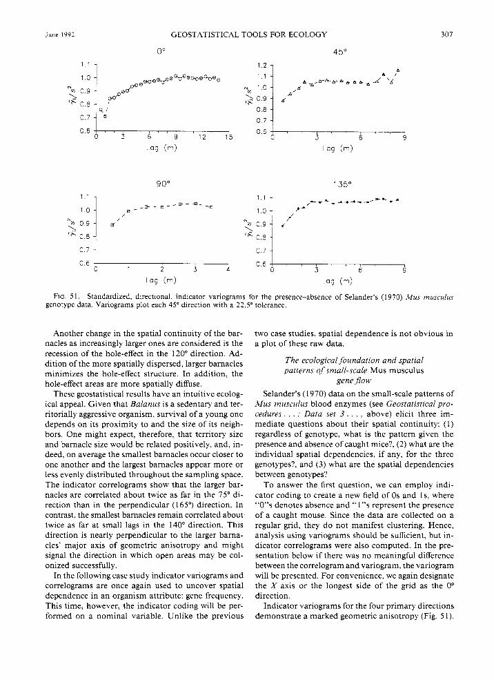
June 1992 GEOSTATISTICAL TOOLS FOR ECOLOGY
0" 4 5 O
307
1 . 1 1 1.2 1 A
0.6 1 0 3 6 9
90" 135"
0.7 1 0.7 i 0.6 ~ I 0.6 1
0 1 2 3 4 0 3 6 9
Lo9 (m) Lag (n)
FIG. 5 1. Standardized, directional, indicator variograms for the presence-absence of Selander's (1 970) Mus rnusculus genotype data. Variograms plot each 45" direction with a 22.5" tolerance.
Another change in the spatial continuity of the bar- nacles as increasingly larger ones are considered is the recession of the hole-effect in the 120" direction. Ad- dition of the more spatially dispersed, larger barnacles minimizes the hole-effect structure. In addition, the hole-effect areas are more spatially diffuse.
These geostatistical results have an intuitive ecolog- ical appeal. Given that Balanus is a sedentary and ter- ritorially aggressive organism, survival of a young one depends on its proximity to and the size of its neigh- bors. One might expect, therefore, that temtory size and barnacle size would be related positively, and, in- deed, on average the smallest barnacles occur closer to one another and the largest barnacles appear more or less evenly distributed throughout the sampling space. The indicator correlograms show that the larger bar- nacles are correlated about twice as far in the 75" di- rection than in the perpendicular (1 65") direction. In contrast, the smallest barnacles remain correlated about twice as far at small lags in the 140" direction. This direction is nearly perpendicular to the larger barna- cles' major axis of geometric anisotropy and might signal the direction in which open areas may be col- onized successfully.
In the following case study indicator variograms and correlograms are once again used to uncover spatial dependence in an organism attribute: gene frequency. This time, however, the indicator coding will be per- formed on a nominal variable. Unlike the previous
two case studies, spatial dependence is not obvious in a plot of these raw data.
The ecological foundation and spatial patterns of small-scale Mus musculus
geneflow Selander's (1 970) data on the small-scale patterns of
Mus musculus blood enzymes (see Geostatistical pro- cedures. . . : Data set 3 . . . , above) elicit three im- mediate questions about their spatial continuity: (1) regardless of genotype, what is the pattern given the presence and absence of caught mice?, (2) what are the individual spatial dependencies, if any, for the three genotypes?, and (3) what are the spatial dependencies between genotypes?
To answer the first question, we can employ indi- cator coding to create a new field of 0 s and Is, where "0"s denotes absence and "1"s represent the presence of a caught mouse. Since the data are collected on a regular grid, they do not manifest clustering. Hence, analysis using variograms should be sufficient, but in- dicator correlograms were also computed. In the pre- sentation below if there was no meaningful difference between the correlogram and variogram, the variogram will be presented. For convenience, we again designate the X axis or the longest side of the grid as the 0" direction.
Indicator variograms for the four primary directions demonstrate a marked geometric anisotropy (Fig. 5 1).

308 RICHARD E. ROSS1 ET AL. Ecological Monographs Vol. 62. No. 2
H om ozyg o us Medium 7
0
-7 7 14 21 28 & ' -23 -21 -14 -7 0
Heterozygous
7 14 21 28 i , ' -28 -21 -14 -7 0
Homozygous Slow
7 14 21 28 A ' -28 -21 -14 -7 0
h in 0"-180" Direction
FIG. 52 . Exhaustive, non-ergodic, indicator correlograms for the three Mus rnusculus genotypes. Original data from Selander (1970). Lag distance is in 0.49 m units.
The range in the 0" direction is over three times as far as in the 90" direction, while ranges in the 45" and 135" directions are slightly longer than the 90" range. Such dramatic differences are lost in Sokal and Oden's (1 978a, b) analysis that mixes different directional cor- relations. Selander originally proposed mouse temto- riality as a mechanism for the obvious heterogeneity between genotypes, but these data consider mouse po- sition regardless of genotype, and suggest that some- thing else is influencing mouse presence and absence.
In a small passage of Selander's paper is a description of the barn environment. Specifically, the chickens are housed in cages that are suspended above the barn floor in rows parallel to the sampling grid's 0" side. The mice, he notes, burrow and nest throughout the mounds of accumulated chicken feces. Hence, the extremely long spatial correlation in the 0" direction is probably due to the availability of this habitat component.
Let us now see whether the availability and orien- tation of this habitat component influences individual genotype spatial patterns. This is accomplished quite simply by indicator coding: 1 s are assigned to locations where a mouse expresses a particular genotype and 0s are coded elsewhere on the grid. Initially these coded
data were analyzed using standardized variograms to permit easier visual inspection between genotypes. However, the resulting sills all occurred beyond the variance value of unity and at different levels. This behavior signals possible differences in local means and variances. That result seems reasonable given that we are analyzing the distribution of a specific gene of an organism that is territorial. Therefore, we might expect, a priori, that any genotype's spatial distribution will be somewhat clumped. As in the last ecological ex- ample, correlograms were then also computed and the results found to be better behaved.
The non-ergodic exhaustive correlograms are flipped in variogram form and model the spatial continuity differences between the genotypes (Fig. 5 2 ) . Although indicator-coded data typically produce spatial-conti- nuity models that have larger nuggets than continuous data, all of the correlogram models have substantial nuggets. Thus, on the one hand, there is likely to be undetected spatial pattern smaller than the 0.5-m sam- ple spacing. On the other hand, the poorer structures are indications that the spatial pattern of the mice, which is strongly influenced by habitat availability, is more prominent than the spatial pattern due to a spe-

June 1992 GEOSTATISTICAL TOOLS FOR ECOLOGY 309
cific genotype. Nevertheless, some specific-if subtle- genotype differences are apparent.
The exhaustive correlograms are noisy, but the im- portant features are the differences between the geno- type ranges. The homozygous medium genotype dem- onstrates a geometric anisotropy with a 60" major axis. Its range in the 0" direction is the shortest of the three. The heterozygous genotype manifests the smallest 90" range, but a narrow 0" range that extends out to a distance of -21 lags or just over 10 m. The homo- zygous slow genotype shows both a long 0" range and a 90" range that goes beyond the maximum significant distance of 7 lags or -3.4 m. It is unknown whether these differences are related to preferences for move- ment because there is no plausible reason why one genotype would show a stronger spatial correlation in any one direction over another. Again, the large nuggets suggest that these genotype differences are due to chance.
Finally, we can model the spatial cross-correlation between genotypes. To do so, our indicator transfor- mation proceeds by coding locations that express one genotype with a '' 1 " and locations expressing another are coded "0." This makes the results conditional on locations having mice of the two genotypes. It also reduces considerably the possibilities of modeling sig- nificant directional variograms because of the smaller number of pairs.
Omnidirectional cross-correlations computed using both the traditional variogram and the non-ergodic correlogram show that the cross-correlograms tend to have smaller nuggets than the cross-variograms (Fig. 53). Curiously, the best structures are achieved when the homozygous medium genotype is paired with either of the other genotypes. If, as Sokal and Oden (1 978b) suggest, more heterozygote-homozygote pairings are expected, the cross-correlograms between these geno- types is likely to demonstrate strong spatial continuity, while a cross-correlogram between the two homozy- gous genotypes would be expected to demonstrate spa- tial independence or pure nugget behavior. On the contrary, it is the homozygous slow-heterozygous cross- correlogram that reflects pure nugget behavior. These results suggest that the locations of or proximity to a mouse with the homozygous medium genotype dom- inate the inter-genotype spatial patterns. This result compliments Sokal and Oden's (1 978b) finding that the autocorrelation between contiguous homozygous medium pairings is strong and positive.
The individual and joint spatial patterns of adult Diabrotica barberi and
Zea mays root damage Our exploratory analysis of Tollefson's data (see
Geostatistical procedure in ecological analysis: Data set 4 . . . , above) of adult rootworms and concomitant damage to corn roots revealed a large difference be- tween the Pearson and Spearman correlation coeffi- cients. This suggested that the spatial relationship be-
1.5 1
m e m Vario r a m ****a CorreTogram
0.0 0 2 4 6 8 10 12 1 4
1.5 1 c
W ~ W Voriogram mmmm. Correlogrom
0.0 0 2 4 6 8 1 0 1 2 1 4
1 ' 5 1.2 3 $ 1 0.6
Homoz. Slow - Heterozygote
fihfi Variogrom 0 . 3 1 , I , LLALA Correlogram , , , , I
0.0 0 2 4 6 8 1 0 1 2 1 4
Log (m)
FIG. 53. Omnidirectional standardized cross-variograms and non-ergodic cross-correlograms between the three AMus musculus genotypes reported by Selander ( 1 970).
310 RICHARD E. ROSS1 ET AL. Ecological Monoerauhs
tween the worm and its host is non-linear, or that data outliers are minimizing the point-to-point correlation, or both. Mindful of these possibilities, we now explore their individual as well as their joint spatial relation- ships geostatistically.
The importance of identifying outliers. -Conditional histograms of the beetle indices for each root rating suggest a positive relationship between the two vari- ables. Two features contribute to a more pronounced relationship: (1) the data represent overlapping cate- gories or rankings of beetle density and root damage, and (2) some locations express a large beetle index but a small root rating, while some others reflect the op- posite. Matching of opposite beetle and root ratings could constitute outliers. Outliers, i.e., unusually large or small values, can be identified. Outliers are of in- terest in modeling spatial variation or cross-correlation using variograms and cross-variograms because both measures average squared differences between data lo- cations. Consequently their values are strongly influ- enced by unusually large or small data.
Identifying outliers may be of interest in ecology regardless of any geostatistical applications. Knowing the locations of unusually large or small concentrations of an organism or an environmental component can improve the ecologist’s ability to understand the un- derlying processes that give rise to and sustain the or- ganism+nvironment relationship. This is especially important in ecological investigations because ecolog- ical variables tend to be unpredictable and to vary spatially and temporally to a great degree. When deal- ing with ecological properties, therefore, outliers may be expected, not merely suspected.
Outliers can be identified through a variety of means. One technique was described earlier: h-scattergram values that plot very far from the 45” line are likely outlier candidates. With this method it is incumbent on the researcher to investigate these possible outliers. For example, does the suspected outlier occur in an area of generally small or large values? Could the un- usual value be an incorrectly coded datum? Is the sus- pected outlier’s presence due to an environmental or organism anomaly? Only after good ecological judg- ment should an outlier be removed prior to variogram analysis. This process can be tedious for large, outlier- laden data sets, but it is perhaps the only legitimate means for outlier identification and removal. With so few rating categories in the present data, outliers will be particularly difficult to explicitly identify.
Many other, more automatic, outlier identification techniques have been proposed. Dowd (1984) can be consulted for reviews of many of the more popular- often called “resistant”-variogram methods, i.e., var- iograms that are resistant to the outliers’ effects. Huber (1964, 1972) provides an excellent statistical exami- nation of outlier-resistant estimation. Some of the more popular resistant variogram techniques are: the me- dium absolute deviation estimator (Dowd 1984, Jour-
- Vol. 62 ,No 2
nel 1984a), generalized distance measures (Journel 1989), median polish (Cressie 1984, 1986), the Cressie- Hawkins estimator (Cressie and Hawkins 1980), and Omre’s estimator (Omre 1984).
Comparisons will be entertained in the next two sub- sections between the h-scattergram cleaning technique and Hawkins’ (1980) method of spatial outlier iden- tification. Hawkins’ method is chosen because it is not linked to variography per se, so the ecologist may use his tool to locate unusually large or small data. His method is also easy to implement. Krige and Magri (1 982) may be consulted for a demonstration of Haw- kins’ method as applied to gold mining data.
Hawkins’ (1 980) spatial outlier detection method. - Hawkins’ approach is straightforward. All values, z(x), are considered a priori suspect. Because spatial outliers are not necessarily the largest or smallest values en- countered, each value is compared to its neighboring values. Let n be defined as the number of neighboring values excluding z(x), let M equal the arithmetic mean of the n values, and let a2 denote the average variance for equivalently sized neighborhoods over the sam- pling space. Assuming the neighborhood values are normally distributed, Hawkins has shown:
(13) n[z(x) - M I 2
( n + l)u2 to be distributed as a x2,. Thus, if the value of Eq. 13 is outside the expected x2 distribution, then that z(x ) value is a spatial outlier.
Resistant rootworm density and variograms of dam- age. -Outliers can completely overwhelm a variogram and mask structure. For example, consider the omni- directional variograms using the raw data for the beetle, the same data after h-scattergram cleaning, and the data after Hawkins’ method has been employed (Fig. 54). All three sets of data appear to show isotropic behavior, so these omnidirectional models are suffi- cient. The variogram of the raw data has a pure nugget structure, and one might conclude that the beetle rating has no spatial dependence, at least at the scale mea- sured. The other, outlier-free variograms tell a different story: these variograms suggest (1) spatial continuity exists at less than the minimum sample spacing of 1.6 km and (2) the ratings demonstrate an average scale of spatial correlation of = 15-18 km. Both outlier-free variograms have very similar structures.
The variogram results of both outlier identification procedures are highly dependent on the conditions im- posed in the analysis. For the h-scattergram cleaning, the ratings that paired the largest differences (i.e., “4” with “0,” “4” with “1,” and “3” with “0”) were ex- cluded from the variogram calculation for all signifi- cant lags. The decision to exclude comparisons be- tween data with the largest differences was based solely on the knowledge that the larger the differences be- tween z(x) and z(x + h), the larger will be the variogram value, especially at small lags. The largest difference
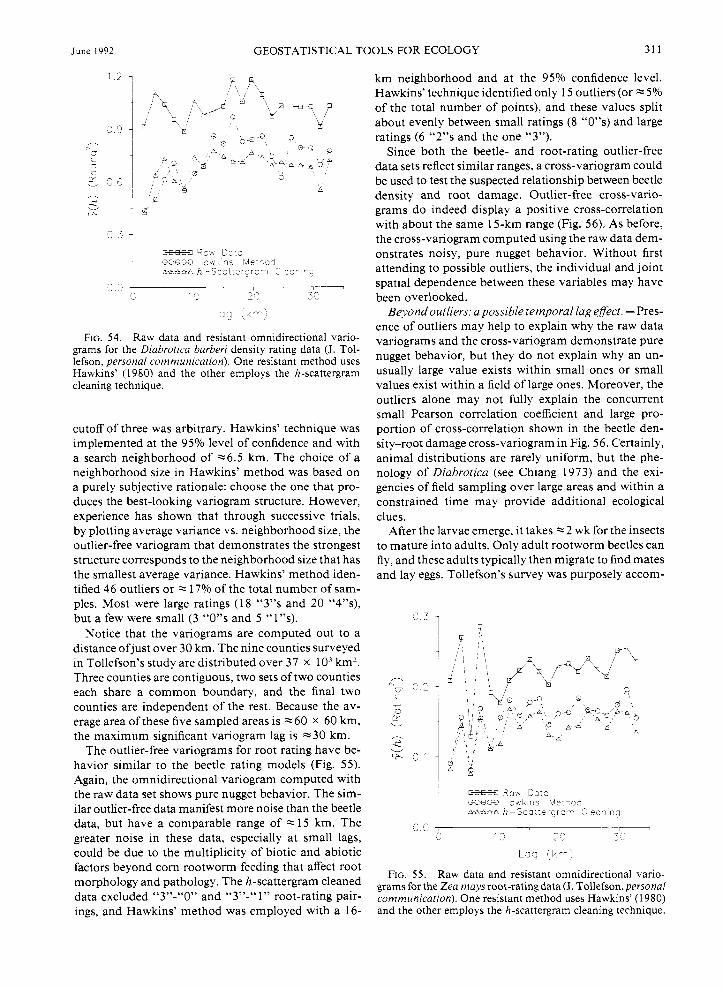
June 1992 GEOSTATISTICAL TOOLS FOR ECOLOGY 31 1
FIG. 54. Raw data and resistant omnidirectional vano- grams for the Diabrotica barberi density rating data (J. Tol- lefson, personal communication). One resistant method uses Hawkins’ ( 1 980) and the other employs the h-scattergram cleaning technique.
cutoff of three was arbitrary. Hawkins’ technique was implemented at the 95% level of confidence and with a search neighborhood of ~ 6 . 5 km. The choice of a neighborhood size in Hawkins’ method was based on a purely subjective rationale: choose the one that pro- duces the best-looking variogram structure. However, experience has shown that through successive trials, by plotting average variance vs. neighborhood size, the outlier-free variogram that demonstrates the strongest structure corresponds to the neighborhood size that has the smallest average variance. Hawkins’ method iden- tified 46 outliers or Z 17% of the total number of sam- ples. Most were large ratings (18 “3”s and 20 “4”s), but a few were small (3 “0”s and 5 “1”s).
Notice that the variograms are computed out to a distance ofjust over 30 km. The nine counties surveyed in Tollefson’s study are distributed over 37 x 1 O 3 km2. Three counties are contiguous, two sets of two counties each share a common boundary, and the final two counties are independent of the rest. Because the av- erage area of these five sampled areas is ~ 6 0 x 60 km, the maximum significant variogram lag is ~ 3 0 km.
The outlier-free variograms for root rating have be- havior similar to the beetle rating models (Fig. 55). Again, the omnidirectional variogram computed with the raw data set shows pure nugget behavior. The sim- ilar outlier-free data manifest more noise than the beetle data, but have a comparable range of z 15 km. The greater noise in these data, especially at small lags, could be due to the multiplicity of biotic and abiotic factors beyond corn rootworm feeding that affect root morphology and pathology. The h-scattergram cleaned data excluded “3”-“0” and “3”-“ 1” root-rating pair- ings, and Hawkins’ method was employed with a 16-
km neighborhood and at the 95% confidence level. Hawkins’ technique identified only 15 outliers (or 5% of the total number of points), and these values split about evenly between small ratings (8 “0”s) and large ratings (6 “2”s and the one “3”).
Since both the beetle- and root-rating outlier-free data sets reflect similar ranges, a cross-variogram could be used to test the suspected relationship between beetle density and root damage. Outlier-free cross-vario- grams do indeed display a positive cross-correlation with about the same 15-km range (Fig. 56). As before, the cross-variogram computed using the raw data dem- onstrates noisy, pure nugget behavior. Without first attending to possible outliers, the individual and joint spatial dependence between these variables may have been overlooked.
Beyond outliers: a possible temporal lag efect. - Pres- ence of outliers may help to explain why the raw data variograms and the cross-variogram demonstrate pure nugget behavior, but they do not explain why an un- usually large value exists within small ones or small values exist within a field of large ones. Moreover, the outliers alone may not fully explain the concurrent small Pearson correlation coefficient and large pro- portion of cross-correlation shown in the beetle den- sity-root damage cross-variogram in Fig. 56. Certainly, animal distributions are rarely uniform, but the phe- nology of Diabrotica (see Chiang 1973) and the exi- gencies of field sampling over large areas and within a constrained time may provide additional ecological clues.
After the larvae emerge, it takes z 2 wk for the insects to mature into adults. Only adult rootworm beetles can fly, and these adults typically then migrate to find mates and lay eggs. Tollefson’s survey was purposely accom-
-, 7 -.,l
I 4
- ? o w Da!c X B 3 f i - c w k i r s lvle i-o: AA**A h - S c a : t e - g r c - 2 e a i i r g
, ^ 7 - ., ., _ “
^ ^ 1,
3 : ^
L 3 g ’k-,
FIG. 55. Raw data and resistant omnidirectional vano- grams for the Zea mays root-rating data (J. Tollefson,persona/ communication). One resistant method uses Hawkins’ (1980) and the other employs the h-scattergram cleaning technique.
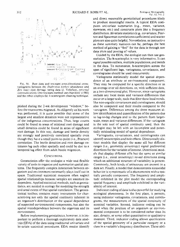
312 RICHARD E. ROSS1 ET AL. Ecological Monographs Vol. 6 2 , No. 2
* ,
c
FIG. 56. Raw data and resistant omnidirectional cross- variograms between the Diabrotica barberi abundance and Zea maj’s root damage rating data (J. Tollefson, personal communication). One resistant method uses Hawkins’ ( 1 980) and the other employs the h-scattergram cleaning technique.
plished during the 2-wk development “window,” be- fore the rootworms migrated. As diligently as his work was performed, it is quite possible that some of the largest and smallest densities were not representative of the indigenous concentrations. Thus, large counts could be found in areas of minimal root damage and small densities could be found in areas of significant root damage. In this way, damage and beetle density are strongly and positively correlated spatially even though they have a small point-to-point (i.e., Pearson) correlation. The beetle densities and root damage es- timates lag each other spatially and could be due to a temporal lag effect from adult beetle migration.
CONCLUSIONS Geostatistics offer the ecologist a wide and flexible
variety of tools to organize and summarize spatial pat- terns. The frequently complex interaction between or- ganism and environment necessarily plays itself out in space. Traditional statistical measures often neglect spatial relationships because samples are assumed in- dependent. Applied statistical methods, such as geosta- tistics, are needed in ecology for modeling the strength and areal extent of that spatial correlation. The geosta- tistical toolbox contains many instruments for char- acterizing not only the spatial continuity inherent in an organism’s distribution or the spatial dependence of suspected environmental components, but also the spatial interdependence between the organism and its environment.
Before implementing geostatistics, however, it is im- portant to perform a thorough exploratory data anal- ysis (EDA) of the data using traditional univariate and bivariate statistical procedures. EDA results identify
and direct reasonable geostatistical procedures likely to produce meaningful results. A typical EDA com- putes univariate summaries (e.g., mean, variance, skewness, etc.) and constructs plots like a frequency distribution. Bivariate statistics ( e g , covariance, Pear- son and Spearman correlations coefficients) and scatter plots are also quite helpful. Nevertheless, as instructive as these summary statistics can be, perhaps the best method of gaining a “feel” for the data is through raw data plots and posting of values.
Guided by the EDA, the ecologist can then use geo- statistics. The h-scatterplot is very informative. It can signal possible outliers, multiple populations, and trends in the data. To summarize, h-scatterplots across the span of significant lags, variograms, covariances, and correlograms should be used concurrently.
Variograms statistically model the spatial depen- dence of an attribute or environmental component. They may be computed for a specific direction or as an average over all directions, or, with sufficient data, as a two-dimensional plot. However, since variograms include any local mean and variance differences that occur on a larger scale, tools that filter these local trends, like non-ergodic covariances and correlograms, should also be computed and their results compared to the variogram. Differences among the three measures al- low identification and quantification of the pattern due to lag-to-lag changes and to the pattern from larger- scale, mean and variance differences. If the variogram is the sole tool of spatial continuity used, then the ecologist may be left with an incomplete and poten- tially misleading model of spatial dependence.
Variograms, covariances, and correlograms can identify anisotropies and hole effects. Directionally dis- tinct models that display the same sill but different ranges (i.e., geometric anisotropy) signal preferential directions for the variable of interest. Directional mod- els that display different sills but the same or similar ranges (i.e., zonal anisotropy) reveal directions along which an additional structure of variability is present. Commonly, both kinds of anisotropy are present in a data set. Finally, a model that demonstrates sinusoidal behavior is symptomatic of a phenomenon with a spa- tially periodic component. The frequency and ampli- tude exhibited in the plot model the corresponding spatial frequency and amplitude exhibited in the vari- able(s) of interest.
Indicator coding of data is also powerful for studying ecological phenomena. In the first place, it permits, using indicator variograms, covariances, and correlo- grams, the measurement of the spatial continuity of nominal variables. Second, indicator coding can be used when the position of an organism or environ- mental component is to be considered rather than its size, density, or some other quantitative or qualitative measure. Third, indicator coding allows specification of the spatial geometry of a particular category or a class in a variable’s frequency distribution. These abil-
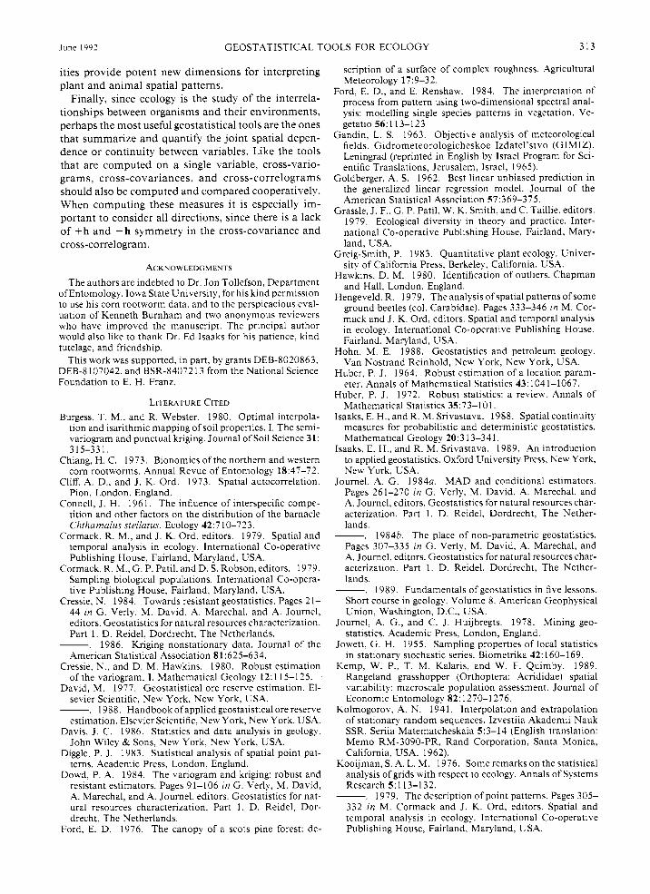
June 1992 GEOSTATISTICAL TOOLS FOR ECOLOGY 313
ities provide potent new dimensions for interpreting plant and animal spatial patterns.
Finally, since ecology is the study of the interrela- tionships between organisms and their environments, perhaps the most useful geostatistical tools are the ones that summarize and quantify the joint spatial depen- dence or continuity between variables. Like the tools that are computed on a single variable, cross-vario- grams, cross-covariances, and cross-correlograms should also be computed and compared cooperatively. When computing these measures it is especially im- portant to consider all directions, since there is a lack of + h and - h symmetry in the cross-covariance and cross-correlogram.
ACKNOWLEDGMENTS The authors are indebted to Dr. Jon Tollefson. Department
of Entomology. Iowa State University, for his kind permission to use his corn rootworm data. and to the perspicacious eval- uation of Kenneth Burnham and two anonymous reviewers who have improved the manuscript. The principal author would also like to thank Dr. Ed Isaaks for his patience. kind tutelage, and friendship.
This work was supported, in part, by grants DEB-8020863. DEB-8 107042. and BSR-8407213 from the National Science Foundation to E. H. Franz.
LITERATURE CITED Burgess, T. M., and R. Webster. 1980. Optimal interpola-
tion and isarithmic mapping of soil properties. I. The semi- variogram and punctual kriging. Journal of Soil Science 31:
Chiang, H. C. 1973. Bionomics of the northern and western corn rootworms. Annual Revue of Entomology 18:47-72.
Cliff. A. D.. and J. K. Ord. 1973. Spatial autocorrelation. Pion, London, England.
Connell, J. H. I96 1. The influence of interspecific compe- tition and other factors on the distribution of the barnacle Chthamalus stellatus. Ecology 42:7 10-723.
Cormack, R. M., and J. K. Ord, editors. 1979. Spatial and temporal analysis in ecology. International Co-operative Publishing House, Fairland, Maryland, USA.
Cormack, R. M., G. P. Patil, andD. S. Robson, editors. 1979. Sampling biological populations. International Co-opera- tive Publishing House, Fairland. Maryland. USA.
Cressie, N. 1984. Towards resistant geostatistics. Pages 2 1- 44 in G. Verly, M. David. A. Marechal, and A. Journel, editors. Geostatistics for natural resources characterization. Part 1 . D. Reidel, Dordrecht, The Netherlands.
-. 1986. Kriging nonstationary data. Journal of the American Statistical Association 81 :625-634.
Cressie, N., and D. M. Hawkins. 1980. Robust estimation of the variogram. I . Mathematical Geology 12: 1 15-125.
David, M. 1977. Geostatistical ore reserve estimation. El- sevier Scientific, New York, New York, USA.
-, 1988. Handbook ofappliedgeostatistical ore reserve estimation. Elsevier Scientific, New York, New York, USA.
Davis, J. C. 1986. Statistics and data analysis in geology. John Wiley & Sons, New York, New York, USA.
Diggle. P. J. 1983. Statistical analysis of spatial point pat- terns. Academic Press, London. England.
Dowd, P. A. 1984. The variogram and kriging: robust and resistant estimators. Pages 91-106 in G. Verly, M. David, A. Marechal, and A. Journel. editors. Geostatistics for nat- ural resources characterization. Part 1. D. Reidel, Dor- drecht. The Netherlands.
1976. The canopy of a scots pine forest: de-
3 1 5-33 1.
Ford, E. D.
scription of a surface of complex roughness. Agricultural Meteorology 17:9-32.
Ford, E. D., and E. Renshaw. 1984. The interpretation of process from pattern using two-dimensional spectral anal- ysis: modelling single species patterns in vegetation. Ve- getatio 56: 1 13-1 23
Gandin, L. S. 1963. Objective analysis of meteorological fields. Gidrometeorologicheskoe Izdatel’stvo (GIMIZ), Leningrad (reprinted in English by Israel Program for Sci- entific Translations, Jerusalem, Israel, 1965).
Goldberger, A. S. 1962. Best linear unbiased prediction in the generalized linear regression model. Journal of the American Statistical Association 57:369-375.
Grassle, J . F.. G. P. Patil, W. K. Smith, and C. Taillie. editors. 1979. Ecological diversity in theory and practice. Inter- national Co-operative Publishing House, Fairland, Mary- land, USA.
Greig-Smith, P. 1983. Quantitative plant ecology. Univer- sity of California Press, Berkeley. California. USA.
Hawkins. D. M. 1980. Identification of outliers. Chapman and Hall, London, England.
Hengeveld. R. 1979. The analysis of spatial patterns of some ground beetles (col. Carabidae). Pages 333-346 in M. Cor- mack and J . K. Ord, editors. Spatial and temporal analysis in ecology. International Co-operative Publishing House. Fairland, Maryland. USA.
Hohn. M. E. 1988. Geostatistics and petroleum geology. Van Nostrand Reinhold, New York, New York, USA.
Huber. P. J . 1964. Robust estimation of a location param- eter. Annals of Mathematical Statistics 43: 104 1-1067.
Huber. P. J . 1972. Robust statistics: a review. Annals of Mathematical Statistics 35:73-10 1.
Isaaks, E. H., and R. M. Srivastava. 1988. Spatial continuity measures for probabilistic and deterministic geostatistics. Mathematical Geology 20:3 13-34 1.
Isaaks, E. H., and R. M. Srivastava. 1989. An introduction to applied geostatistics. Oxford University Press, New York, New York, USA.
Journel, A. G. 1984a. MAD and conditional estimators. Pages 261-270 in G. Verly, M. David. A. Marechal, and A. Journel, editors. Geostatistics for natural resources char- acterization. Part I . D. Reidel, Dordrecht, The Nether- lands.
-, 19846. The place of non-parametric geostatistics. Pages 307-335 in G. Verly, M. David, A. Marechal, and A. Journel, editors. Geostatistics for natural resources char- acterization. Part 1. D. Reidel, Dordrecht, The Nether- lands.
-. 1989. Fundamentals of geostatistics in five lessons. Short course in geology. Volume 8. American Geophysical Union, Washington, D.C., USA.
Journel, A. G., and C. J. Huijbregts. 1978. Mining geo- statistics. Academic Press, London, England.
Jowett, G. H. 1955. Sampling properties of local statistics in stationary stochastic series. Biometrika 42: 160-169.
Kemp, W. P., T. M. Kalaris, and W. F. Quimby. 1989. Rangeland grasshopper (Orthoptera: Acrididae) spatial variability: macroscale population assessment. Journal of Economic Entomology 82: 1270-1276.
Kolmogorov, A. N. 194 1. Interpolation and extrapolation of stationary random sequences. Izvestiia Akademii Nauk SSR. Seriia Matematcheskaia 5:3-14 (English translation: Memo RM-3090-PR, Rand Corporation, Santa Monica, California, USA. 1962).
Kooijman, S. A. L. M. 1976. Some remarks on the statistical analysis of grids with respect to ecology. Annals of Systems Research 5:113-132.
. 1979. The description ofpoint patterns. Pages 305- 332 in M. Cormack and J. K. Ord, editors. Spatial and temporal analysis in ecology. International Co-operative Publishing House, Fairland, Maryland, USA.
Krige, D. G., and E. J . Magri. 1982. Studies of the effects of outliers and data transformation on variogram estimates for a base metal and a gold ore body. Mathematical Geology
Langsaeter, A. 1926. Om beregning av middelfeilen ved regelmessige linjetakseringer. Meddelanden fra det Skog- forsoksvesen, 2h. 7:5-47.
Mattrn, 9. 1947. Metoder att uppskatta noggramheten vid linje-och provytetaxering. Meddelanden f r in Statens Skogsforskningsinstitut 36( I) .
-. 1960. Spatial variation. Springer-Verlag, New York, New York, USA.
Matheron, G . 1963. Principles of geostatistics. Economic Geology 58:1246-1266.
-. 1965. Les variables rtgionalistes et leur estimation. Masson. Pans. France.
McNaughton, S. J., and L. L. Wolf. 1973. General ecology. Holt, Rinehart & Winston, New York, New York, USA.
Odum, E. P. 1975. Ecology: the link between the natural and the social sciences. Holt, Rinehart & Winston, New York, New York, USA.
Olea, R. A.. editor. 1990. Geostatistical glossary and mul- tilingual dictionary. Oxford University Press, New York, New York, USA.
Omre, H. 1984. The variogram and its estimation. Pages 107-125 in G . Verly, M. David, A. Marechal, and A. Jour- nel, editors. Geostatistics for natural resources character- ization. Part I . D. Reidel, Dordrecht, The Netherlands.
Ord, J. K., G. P. Patil, and C. Taillie, editors. 1979. Statis- tical distributions in ecological work. International Co-op- erative Publishing House, Fairland, Maryland, USA.
Orloci, L., C. R. Rao. and W. M. Stiteler, editors. 1979. Multivariate methods in ecological work. International Co- operative Publishing House, Fairland, Maryland, USA.
Patil, G. P., E. C. Pielou, and W. E. Waters, editors. 1 9 7 1 ~ . Spatial patterns and statistical distributions. International Co-operative Publishing House, Fairland, Maryland, USA.
Patil, G. P., E. C. Pielou, and W. E. Waters, editors. 19716. Sampling and modeling biological populations and popu- lation dynamics. International Co-operative Publishing House, Fairland, Maryland, USA.
Patil, G. P., E. C. Pielou, and W. E. Waters, editors. 1 9 7 1 ~ . Many species populations, ecosystems, and systems anal- ysis. International Co-operative Publishing House, Fair- land, Maryland, USA.
Pielou, E. C. 1977. Mathematical ecology. John Wiley & Sons, New York, New York, USA.
Philips, J . D. 1985. Measuring complexity ofenvironmental gradients. Vegetatio 6:95-102.
Platt, T., and K. L. Denman. 1975. Spectral analysis in ecology. Annual Review of Ecology and Systematics 6: 189- 210.
Rendu, J. M. 198 1. An introduction to geostatistical meth- ods of mineral evaluation. South African Institute of Min- ing and Metallurgy, Johannesburg, [Transvaal, Republic of] South Africa.
Renshaw, E. 1984. Competition experiments for light in a plant monoculture: an analysis based on two-dimensional sDectra. Biometrics 40:7 17-728.
1 4 3 5 7-5 64.
RICHARD E. ROSS1 ET AL. Ecological Monographs Vol. 62. No. 2
3 14
spatial pattern using two-dimensional spectral analysis. Ve- getatio 56:75-8 5.
Ricklefs, R. E. 1973. Ecology. Chiron Press, Newton, Mas- sachusetts, USA.
Ripley, 9 . D. 1978. Spectral analysis and the analysis of pattern in plant communities. Journal of Ecology 66:965- 981.
, 198 1. Spatial statistics. John Wiley & Sons, New York, New York, USA.
. 1988. Statistical inference for spatial processes. Cambridge University Press, Cambridge, England.
Robertson, G. P. 1987. Geostatistics in ecology: interpo- lating with known variance. Ecology 68:744-748.
Schotzko, D. J. , and L. E. O’Keeffe. 1989. Geostatistical description of the spatial distribution of Lygus hesperus (Heteroptera: Miridae) in lentils. Journal of Economic En- tomology 82: 1277-1288.
Selander, R. K. 1970. Behavior and genetic variation in natural populations. American Zoologist 10:53-66.
Shugart, H. H., editor. 1978. Proceedings ofthe SIMS Con- ference on Time Series and Ecological Processes. Society for Industrial and Applied Mathematics, Philadelphia, Pennsylvania, USA.
Sokal, R. R., and N. L. Oden. 1 9 7 8 ~ . Spatial autocorrelation in biology. 1. Methodology. Biological Journal of the Lin- nean Society 10: 199-228.
Sokal, R. R., andN. L. Oden. 19786. Spatial autocorrelation in biology. 2. Some biological implications and four ap- plications of evolutionary and ecological interest. Biological Journal of the Linnean Society 10:229-249.
Srivastava, R. M., and H. M. Parker. 1989. Robust mea- sures ofspatial continuity. Pages 295-308 in M. Armstrong, editor. Geostatistics. Volume 1. Kluwer Academic, Dor- drecht, The Netherlands.
Taylor, L. R. 1984. Assessing and interpreting the spatial distributions of insect populations. Annual Review of En- tomology 20:321-357.
Thiele, H. U. 1977. Carabid beetles in their environment. Springer-Verlag, Berlin, Germany.
Tukey, J. 1977. Exploratory data analysis. Addison-Wesley, Reading, Massachusetts, USA.
Vieira, S. R., J. L. Hatfield, D. R. Nielsen, and J. W. Biggar. 1983. Geostatistical theory and application to variability of some agronomical properties. Hilgardia 51: 1-75.
Webster, R. 1985. Quantitative spatial analysis of soil in the field. Advances in Soil Science 3: 1-70.
Whittle, P. 1954. On stationary processes in the plane. Biometrica 41:434449.
-. 1956. On the variation of yield variance with plot size. Biometrica 43:337-343.
-. 1963. Prediction and regulation. English Univer- sities Press, London, England.
Wiener, N. 1949. Extrapolation, interpolation, and smooth- ing of stationary time series. MIT Press, Cambridge, Mas- sachusetts, USA.
Wold, H. 1938. A study in the analysis of stationary time series. Almqvist and Wiksells, Uppsala, Sweden.
Yaglom, A. M. 1957. Some classes of random fields in n-dimensional space related to stationary random process-
Renshaw, E., and E. D. Ford. 1984. The description of es. Theory of Probability and its Applications 2:273-320.