geothermal utilization production power

Presented at “Short Course VI on Utilization of Low- and Medium-Enthalpy Geothermal Resources and Financial Aspects of Utilization”, organized by UNU-GTP and LaGeo, in Santa Tecla, El Salvador, March 23-29, 2014.

LaGeo S.A. de C.V. GEOTHERMAL TRAINING PROGRAMME

GEOTHERMAL UTILIZATION – PRODUCTION OF POWER

Dr. Páll Valdimarsson Reykjavik University / Atlas Copco GAP Geothermal competence Center

Reykjavik / Cologne ICELAND / GERMANY

[email protected] / [email protected]

ABSTRACT This manuscript covers the thermodynamics of power production from a geothermal resource, as well as analysis of the most common cycles and components. A treatment of the economics of geothermal power plants is as well included. This manuscript is intended as background material for the lectures of the author at this Short Course.

1. THERMODYNAMICS OF GEOTHERMAL POWER PRODUCTION 1.1 Energy and power, heat and work The production of electricity from a geothermal source is about producing work from heat. Electricity production from heat will never be successful unless appropriate respect is paid to the second law of thermodynamics. Energy is utilized in two forms, as heat and as work. Work moves bodies, changes their form, but heat changes temperature (changes the molecular random kinetic energy). Work is thus the ordered energy, whereas heat is the random “unorganized” energy. Heat and work are totally different products for a power station, but these two energy forms cannot be produced independent of each other. Independent production of heat and work is in a way similar to have cattle producing three hind legs per animal when required. It is as well appropriate to discuss the relation between power and energy right here in the introduction to this chapter. A power station is built to be able to supply certain maximum power. The source heat supply and the design of the power plant internals are based on this maximum power (Figure 1). On the other hand the income of the power station will be depending on the energy sold, on the integral of produced power with respect to time. Geothermal installations have normally zero energy cost. The inflow into the well is not charged for. The only cost is the investment cost in equipment and installations to get the fluid to the surface, and to process it appropriately in the power plant in order to obtain the product, be it heat for a direct use application or an electricity producing power plant. As a consequence of this, a geothermal power plant is a typical base load plant, the bulk portion of the cost is there regardless of how much power the plant is producing. Duration curves and utilization time will be discussed later in this chapter.

1

Valdimarsson 2 Geothermal utilization - Production of power

FIGURE 1: Schematic of a geothermal power plant 2. CONVERSION OF HEAT TO WORK Work can always be changed into heat. Even during the Stone Age, work was used to light fire by friction, by rubbing wood sticks to a hard surface. The same applies today, the electric heater is converting work into heat with 100% efficiency. Conversion of heat into work is difficult and is limited by the laws of thermodynamics. A part of the heat used has always to be rejected to the surroundings, so there is always an upper limit of the possible work production from a given heat stream. Textbooks use the Reversible Heat Engine (RHE, Carnot engine) as a reference (Figure 2). RHE is the best engine for producing work from heat, assuming that the engine is operating between two infinitely large heat reservoirs. The reference to the Carnot engine has to be taken with caution, as the real heat reservoirs are usually not infinitely large, and the heat supply or rejection will happen at a variable temperature. 2.1 Exergy The second law of thermodynamics demands that a part of the heat input to any heat engine is rejected to the environment. The portion of the input heat, which can be converted into work, is called Exergy (availability, convertible energy). The unconvertible portion is called Anergy. Thus the exergy of any system or flow stream is equal to the maximum work (or electricity) which can be produced from the source. The thermodynamic definition of exergy for a flow stream is: (1) The zero index refers to the environmental conditions for the subject conversion. The local environment for the power plant defines the available cold heat reservoir, and all the anergy rejected tot the environment will finally be at the environmental conditions.

( )0 0 0x h h T s s= − − −

FIGURE 2: The Carnot engine

Geothermal utilization - Production of power 3 Valdimarsson

The exergy of a flow stream is thus the maximum theoretical work which can be produced if the stream is subjected to a process bringing it down to the environmental conditions. If the stream is a liquid with constant heat capacity, the above equation can be written as:

(2)

Economics of power production are conveniently analyzed by using exergy. A power plant has the main purpose of converting heat into work, and therefore the relevant physical variable for cost and economic performance calculation is the exergy rather than the total energy or the heat flow. 2.2 Efficiency definitions Efficiency is the ratio of input to output, a performance measure for the process. There are many possibilities of defining input and output, but the most standard definition of efficiency is the power plant thermal efficiency. Figure 3 shows the energy streams for a binary power plant.

FIGURE 3: Energy streams in a binary power plant The thermal efficiency is seen as the ratio of produced power to the heat transferred to the power plant. The effectiveness is the ratio of the heat transferred to the power plant to the heat available from the wells. It is obvious that the total power plant efficiency will be the multiple of power plant efficiency and effectiveness. 2.3 Power plant thermal efficiency The power plant thermal efficiency is the ratio between power produced and the heat flow to the power plant. The power plant thermal efficiency is traditionally defined as:

(3)

( )0 00

lnliquidTx c T T TT

= − −

Heat from wells

Heat from generation

Produced power

Heat re-injected

Heat to powerplant

thin

WQ

η =

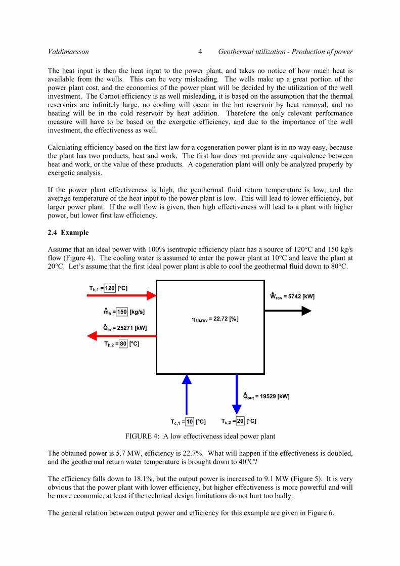
Valdimarsson 4 Geothermal utilization - Production of power The heat input is then the heat input to the power plant, and takes no notice of how much heat is available from the wells. This can be very misleading. The wells make up a great portion of the power plant cost, and the economics of the power plant will be decided by the utilization of the well investment. The Carnot efficiency is as well misleading, it is based on the assumption that the thermal reservoirs are infinitely large, no cooling will occur in the hot reservoir by heat removal, and no heating will be in the cold reservoir by heat addition. Therefore the only relevant performance measure will have to be based on the exergetic efficiency, and due to the importance of the well investment, the effectiveness as well. Calculating efficiency based on the first law for a cogeneration power plant is in no way easy, because the plant has two products, heat and work. The first law does not provide any equivalence between heat and work, or the value of these products. A cogeneration plant will only be analyzed properly by exergetic analysis. If the power plant effectiveness is high, the geothermal fluid return temperature is low, and the average temperature of the heat input to the power plant is low. This will lead to lower efficiency, but larger power plant. If the well flow is given, then high effectiveness will lead to a plant with higher power, but lower first law efficiency. 2.4 Example Assume that an ideal power with 100% isentropic efficiency plant has a source of 120°C and 150 kg/s flow (Figure 4). The cooling water is assumed to enter the power plant at 10°C and leave the plant at 20°C. Let’s assume that the first ideal power plant is able to cool the geothermal fluid down to 80°C.

FIGURE 4: A low effectiveness ideal power plant The obtained power is 5.7 MW, efficiency is 22.7%. What will happen if the effectiveness is doubled, and the geothermal return water temperature is brought down to 40°C? The efficiency falls down to 18.1%, but the output power is increased to 9.1 MW (Figure 5). It is very obvious that the power plant with lower efficiency, but higher effectiveness is more powerful and will be more economic, at least if the technical design limitations do not hurt too badly. The general relation between output power and efficiency for this example are given in Figure 6.

Tc,1 = 10 [°C] Tc,2 = 20 [°C]

Th,1 = 120 [°C]

Th,2 = 80 [°C]

mh = 150 [kg/s]

Qin = 25271 [kW]

Qout = 19529 [kW]

Wrev = 5742 [kW]

η th,rev = 22,72 [%]


FIGURE 5: A high effectiveness ideal power plant

FIGURE 6: Net power and efficiency as a function of re-injection temperature 2.5 Effectiveness The power plant effectiveness is the ratio between the available energy to the energy input to the power plant. The available energy is found by assuming that the geothermal fluid can be cooled down to the environmental conditions. Effectiveness will be the deciding factor for the possible power plant size, rather than the quality of the power plant. 2.6 Second law efficiency and effectiveness Exergy is the portion of the energy which can theoretically be converted into work. It is logical to base performance criteria for production of electricity on exergy rather than heat or energy, because then the performance calculation will take into account what can be done, and not incorporate any “perpetuum mobile” in the calculations.

Tc,1 = 10 [°C] Tc,2 = 20 [°C]

Th,1 = 120 [°C]

Th,2 = 40 [°C]

mh = 150 [kg/s]

Qin = 50340 [kW]

Qout = 41235 [kW]

Wrev = 9105 [kW]

η th,rev = 18,09 [%]

40 45 50 55 60 65 70 75 80 8518

19

20

21

22

23

24

5000

5500

6000

6500

7000

7500

8000

8500

9000

9500

Geothermal fluid return temperature [°C]

ηth

;re v

[%]

Wre

v [k

W]

Valdimarsson 6 Geothermal utilization - Production of power The second law approach makes as well easy to treat cogeneration. Then the exergy stream in the sold heat is treated in the same way as the produced electrical power, having the same exergy unitary cost. 3. ANALYSIS Efficiency is the ratio of benefit to cost. In order to be able to define efficiency, the inputs (cost) and outputs have to be defined. In a low temperature heat conversion process, two cases regarding the stream are possible, depending on if the heat contained in that stream can be sold to a heat consuming process. The conversion efficiency is a measure of how much of the available heat is converted into work. It has to be kept in mind that only a part of the heat can be converted into work due to the limitations imposed by the second law of thermodynamics. Exergy, the potential of any system to produce work, is the correct property to consider, when the conversion efficiency is analyzed. Exergy is dependent of the properties of the source as well as the properties of the environment, where the environmental temperature and pressure are the main properties. The temperature of the entering cooling fluid is taken to be the environmental temperature, the lowest temperature which can be obtained, as well as defining the thermal sink temperature for the Carnot engine efficiency. The environmental pressure is logically the ambient atmospheric pressure This process can be seen as a non-conserving heat exchange process between the source stream and the cooling fluid stream. Figure 7 is a block diagram of a power plant converting heat into electricity.

FIGURE 7: Electrical power plant schematic The variables related to the conversion are as follows:

ch = Source fluid heat capacity; mh = Flow rate of source fluid; Th = Source fluid inlet temperature; Ts = Source fluid outlet temperature; cc = Cooling fluid heat capacity; mc = Cooling fluid flow rate; Tc = Cooling fluid outlet temperature; and T0 = Cooling fluid inlet temperature (Environmental temperature).


In the following this system will be analyzed in order to gain a better understanding of the conversion of low temperature heat into electricity. It is assumed that the geothermal source fluid is liquid water with constant heat capacity. The streams in and out of the system have four flow properties: mass, heat capacity, enthalpy and exergy. The mass conservation is obvious, no mixing of the source and cooling streams is assumed. The heat capacity is important for the characteristics of the heat conversion, and will be treated here as a heat capacity flow, the product of fluid heat capacity and flow rate. The product of the enthalpy relative to the environmental temperature and the flow rate defines the heat flow in and out of the system. The exergy will give information on the work producing potential of the system, and is calculated in the same way as the enthalpy. Reference textbooks such as Cengel (2002) give basic information on exergy and its definition, but here the analysis is as well based on Kotas (1985) and Szargut (1988). Thórólfsson (2002), Valdimarsson (2002) and Dorj (2005) apply these methods on specific geothermal applications. The heat ( ) and exergy ( ) flows are given by:

(4)

(5)

(6)

(7)

(8)

(9)

The energy (1. law) and exergy (2. law) balances are:

(10)

or:

(11)

The energy balance is valid for all processes, ideal and real. The exergy balance gives only information on the reversible work, or the largest amount of work that can be obtained from the power plant.

Q X

( )0TTmcQ hhhh −=

( )0TTmcQ shhs −=

( )0TTmcQ cccc −=

( )0 0 00 0

ln lnh hh h h h h h h

T TX c m T T T Q c m TT T

= − − = −

( )

−=

−−=

00

000 lnln

TTTmcQ

TTTTTmcX s

hhss

shhs

( )

−=

−−=

00

000 lnln

TTTmcQ

TTTTTmcX c

cccc

cccc

WQQQ csh =−−

revcsh WXXX =−−

revc

ccs

hhhcsh W

TTTmc

TTTmcQQQ =

+

−−−

000 lnln

Valdimarsson 8 Geothermal utilization - Production of power If the power plant is ideal, then:

(12)

Then the heat capacity flow ratio for a reversible power plant is:

(13)

Assume that electricity is the only output of the power plant. The heat contained in the stream is rejected to the surroundings.

First law efficiency:

(14)

First law maximum efficiency:

(15)

0lnln0

00 =

+

−=

TT

TmcTT

TmcorWW ccc

s

hhhrev

==

0

ln

ln

TTTT

mcmcC

c

s

h

revhh

ccrev

cs

h

QandQ

QW

:Rejected

:Input:Product

( ) ( )0

0, TT

TTCTTQ

QQQQW

h

csh

h

csh

hEI −

−−−=

−−==

η

h

ccc

s

hhhcs

h

csh

h

revEI Q

TTTmc

TTTmcQQ

QXXX

QW

−

++

−=−−

== 000

max,,

lnln1η

( )

( )

( )

( )0

000

0

0 lnln

TTTT

TTTC

TTTT

TTT

h

cc

h

s

hsh

−

−−

−−

−−

=

( ) ( )

( )00

00

ln

lnln

TTTT

TTTTTT

TT

hc

cs

hsh

c

−

−

−−

=


Second law efficiency:

(16)

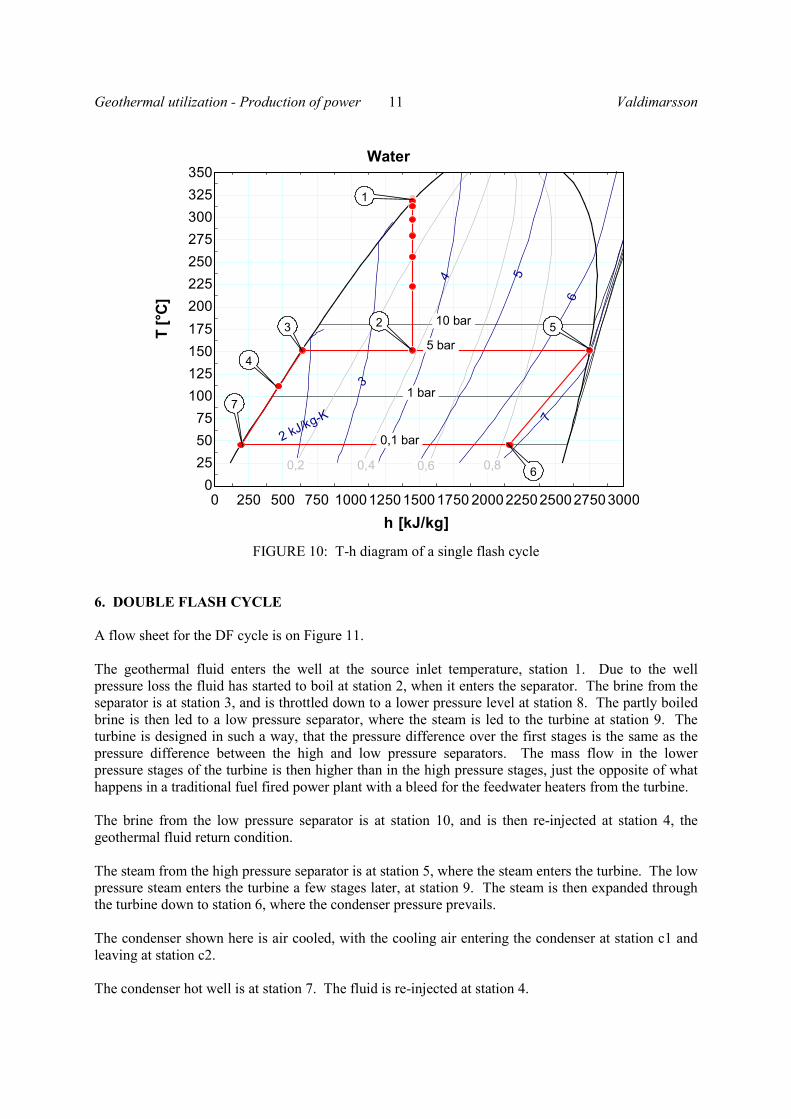
4. POWER PLANT TYPES The geothermal power plants can be divided into two main groups, steam cycles and binary cycles. Typically the steam cycles are used at higher well enthalpies, and binary cycles for lower enthalpies. The steam cycles allow the fluid to boil, and then the steam is separated from the brine and expanded in a turbine. Usually the brine is rejected to the environment (re-injected), or it is flashed again at a lower pressure. Here the Single Flash (SF) and Double Flash (DF) cycles will be presented. A binary cycle uses a secondary working fluid in a closed power generation cycle. A heat exchanger is used to transfer heat from the geothermal fluid to the working fluid, and the cooled brine is then rejected to the environment or re-injected. The Organic Rankine Cycle (ORC) and Kalina cycle will be presented. 5. SINGLE FLASH CYCLE A flow sheet for the SF cycle is shown in Figure 8. The geothermal fluid enters the well at the source inlet temperature, station 1. Due to the well pressure loss the fluid has started to boil at station 2, when it enters the separator. The brine from the separator is at station 3, and is re-injected at station 4, the geothermal fluid return condition. The steam from the separator is at station 5, where the steam enters the turbine. The steam is then expanded through the turbine down to station 6, where the condenser pressure prevails. The condenser shown here is air cooled, with the cooling air entering the condenser at station c1 and leaving at station c2. The condenser hot well is at station 7. The fluid is re-injected at station 4. Typically, such a process is displayed on a thermodynamic T-s diagram, where the temperature in the cycle is plotted against the entropy (Figure 9). A T-h diagram is shown in Figure 10. The condition at station 1 is usually compressed liquid. In vapour dominated fields, such as Lardarello in Italy, the inflow is in the wet region close to the vapour saturation line.

+

−−−

−−=

−−−−

==

000

,

lnlnTTTmc

TTTmcQQQ

QQQXXXQQQ

WW

ccc

s

hhhcsh

csh

csh

csh

revEII

η

( ) ( )

( ) ( )

−−−

−−

−−−=

0000

0

lnlnTT

TTTCTT

TTT

TTCTT

cc

s

hsh

csh


FIGURE 8: Single flash cycle schematic

FIGURE 9: T-s diagram of a single flash cycle

2

5

3

6

7

Production well

Separator

Turbine

Condenser

c1

c2

Condenserpump

Re-injectionpump

1

4

0,0 1,0 2,0 3,0 4,0 5,0 6,0 7,0 8,0 9,0 10,00

255075

100125150175200225250275300325350

s [kJ/kg-K]

T [°

C]

10 bar

5 bar

1 bar

0,1 bar

0,2 0,4 0,6 0,8

Water

1

23 5

6

7

4


FIGURE 10: T-h diagram of a single flash cycle 6. DOUBLE FLASH CYCLE A flow sheet for the DF cycle is on Figure 11. The geothermal fluid enters the well at the source inlet temperature, station 1. Due to the well pressure loss the fluid has started to boil at station 2, when it enters the separator. The brine from the separator is at station 3, and is throttled down to a lower pressure level at station 8. The partly boiled brine is then led to a low pressure separator, where the steam is led to the turbine at station 9. The turbine is designed in such a way, that the pressure difference over the first stages is the same as the pressure difference between the high and low pressure separators. The mass flow in the lower pressure stages of the turbine is then higher than in the high pressure stages, just the opposite of what happens in a traditional fuel fired power plant with a bleed for the feedwater heaters from the turbine. The brine from the low pressure separator is at station 10, and is then re-injected at station 4, the geothermal fluid return condition. The steam from the high pressure separator is at station 5, where the steam enters the turbine. The low pressure steam enters the turbine a few stages later, at station 9. The steam is then expanded through the turbine down to station 6, where the condenser pressure prevails. The condenser shown here is air cooled, with the cooling air entering the condenser at station c1 and leaving at station c2. The condenser hot well is at station 7. The fluid is re-injected at station 4.

0 250 500 750 1000125015001750 200022502500275030000

255075

100125150175200225250275300325350

h [kJ/kg]

T [°

C]

10 bar

5 bar

1 bar

0,1 bar

0,2 0,4 0,6 0,8

7

6

5

4

3

2 kJ/kg-K

Water

1

23 5

6

7

4


FIGURE 11: Double flash cycle schematic The double flash cycle is presented in Figure 12 on a T-s diagram and on a T-h diagram on Figure 13.

FIGURE 12: T-s diagram of a double flash cycle

2

5

3

6

7

Production well

Highpressureseparator

Turbine

Condenser

c1

c2

Condenserpump

Re-injectionpump

1

4

8

9

Lowpressureseparator

Throttlingvalve

10

0,0 1,0 2,0 3,0 4,0 5,0 6,0 7,0 8,0 9,0 10,00

255075

100125150175200225250275300325350

s [kJ/kg-K]

T [°

C]

10 bar

5 bar

1 bar

0,1 bar

0,2 0,4 0,6 0,8

Water

1

235

67

49

8

10


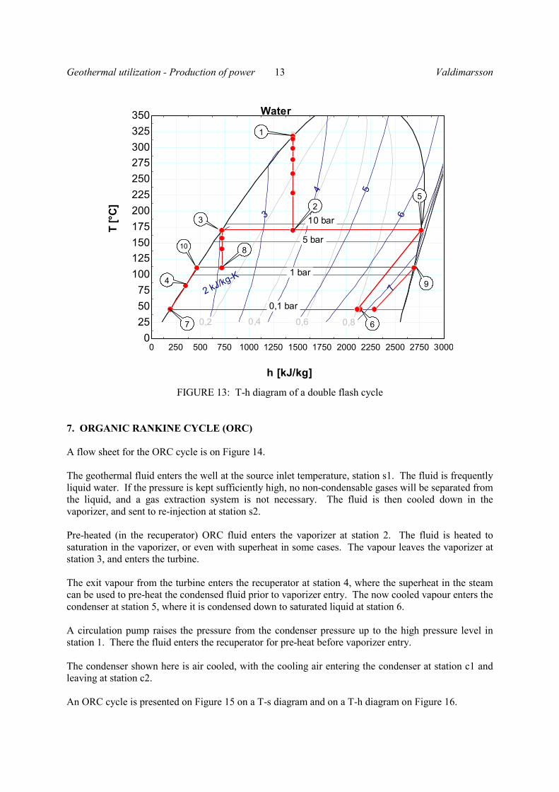
FIGURE 13: T-h diagram of a double flash cycle 7. ORGANIC RANKINE CYCLE (ORC) A flow sheet for the ORC cycle is on Figure 14. The geothermal fluid enters the well at the source inlet temperature, station s1. The fluid is frequently liquid water. If the pressure is kept sufficiently high, no non-condensable gases will be separated from the liquid, and a gas extraction system is not necessary. The fluid is then cooled down in the vaporizer, and sent to re-injection at station s2. Pre-heated (in the recuperator) ORC fluid enters the vaporizer at station 2. The fluid is heated to saturation in the vaporizer, or even with superheat in some cases. The vapour leaves the vaporizer at station 3, and enters the turbine. The exit vapour from the turbine enters the recuperator at station 4, where the superheat in the steam can be used to pre-heat the condensed fluid prior to vaporizer entry. The now cooled vapour enters the condenser at station 5, where it is condensed down to saturated liquid at station 6. A circulation pump raises the pressure from the condenser pressure up to the high pressure level in station 1. There the fluid enters the recuperator for pre-heat before vaporizer entry. The condenser shown here is air cooled, with the cooling air entering the condenser at station c1 and leaving at station c2. An ORC cycle is presented on Figure 15 on a T-s diagram and on a T-h diagram on Figure 16.

0 250 500 750 1000 1250 1500 1750 2000 2250 2500 2750 30000

255075

100125150175200225250275300325350

h [kJ/kg]

T [°

C]

10 bar

5 bar

1 bar

0,1 bar

0,2 0,4 0,6 0,8

7

6

5

4

3

2 kJ/kg-K

Water

1

23

5

67

4 9

810


FIGURE 14: Flow diagram for an ORC cycle with recuperation

FIGURE 15: T-s diagram of an ORC cycle with recuperation

1

6

5

2

3

4

s1

s2

c1

c1

Vaporizer

Turbine

Regenerator

Air-cooledcondenser

Circulationpump

-1,8 -1,5 -1,2 -0,9 -0,6 -0,3 0,00

25

50

75

100

125

150

175

200

s [kJ/kg-K]

T [°

C]

25 bar

15 bar

5 bar

1 bar

0,2 0,4 0,6 0,8

Isopentane

1

2

3

56

4


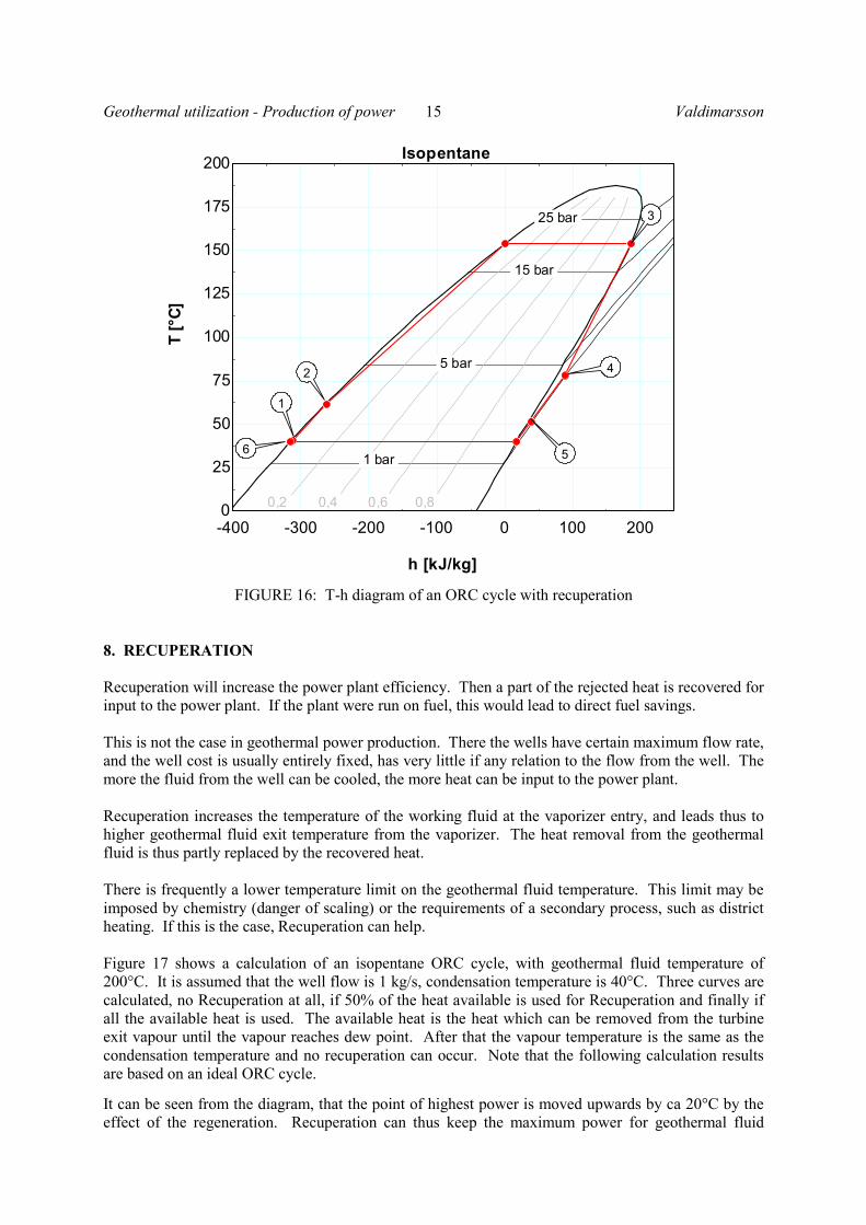
FIGURE 16: T-h diagram of an ORC cycle with recuperation 8. RECUPERATION Recuperation will increase the power plant efficiency. Then a part of the rejected heat is recovered for input to the power plant. If the plant were run on fuel, this would lead to direct fuel savings. This is not the case in geothermal power production. There the wells have certain maximum flow rate, and the well cost is usually entirely fixed, has very little if any relation to the flow from the well. The more the fluid from the well can be cooled, the more heat can be input to the power plant. Recuperation increases the temperature of the working fluid at the vaporizer entry, and leads thus to higher geothermal fluid exit temperature from the vaporizer. The heat removal from the geothermal fluid is thus partly replaced by the recovered heat. There is frequently a lower temperature limit on the geothermal fluid temperature. This limit may be imposed by chemistry (danger of scaling) or the requirements of a secondary process, such as district heating. If this is the case, Recuperation can help. Figure 17 shows a calculation of an isopentane ORC cycle, with geothermal fluid temperature of 200°C. It is assumed that the well flow is 1 kg/s, condensation temperature is 40°C. Three curves are calculated, no Recuperation at all, if 50% of the heat available is used for Recuperation and finally if all the available heat is used. The available heat is the heat which can be removed from the turbine exit vapour until the vapour reaches dew point. After that the vapour temperature is the same as the condensation temperature and no recuperation can occur. Note that the following calculation results are based on an ideal ORC cycle.

It can be seen from the diagram, that the point of highest power is moved upwards by ca 20°C by the effect of the regeneration. Recuperation can thus keep the maximum power for geothermal fluid

-400 -300 -200 -100 0 100 2000

25

50

75

100

125

150

175

200

h [kJ/kg]

T [°

C]

25 bar

15 bar

5 bar

1 bar

0,2 0,4 0,6 0,8

Isopentane

1

2

3

56

4

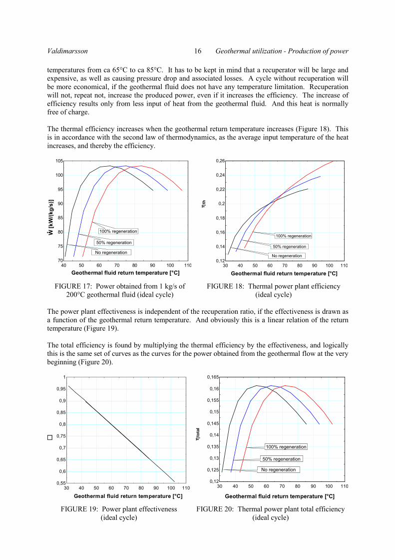
Valdimarsson 16 Geothermal utilization - Production of power temperatures from ca 65°C to ca 85°C. It has to be kept in mind that a recuperator will be large and expensive, as well as causing pressure drop and associated losses. A cycle without recuperation will be more economical, if the geothermal fluid does not have any temperature limitation. Recuperation will not, repeat not, increase the produced power, even if it increases the efficiency. The increase of efficiency results only from less input of heat from the geothermal fluid. And this heat is normally free of charge. The thermal efficiency increases when the geothermal return temperature increases (Figure 18). This is in accordance with the second law of thermodynamics, as the average input temperature of the heat increases, and thereby the efficiency.

FIGURE 17: Power obtained from 1 kg/s of 200°C geothermal fluid (ideal cycle)

FIGURE 18: Thermal power plant efficiency (ideal cycle)

The power plant effectiveness is independent of the recuperation ratio, if the effectiveness is drawn as a function of the geothermal return temperature. And obviously this is a linear relation of the return temperature (Figure 19). The total efficiency is found by multiplying the thermal efficiency by the effectiveness, and logically this is the same set of curves as the curves for the power obtained from the geothermal flow at the very beginning (Figure 20).

FIGURE 19: Power plant effectiveness (ideal cycle)

FIGURE 20: Thermal power plant total efficiency (ideal cycle)

40 50 60 70 80 90 100 11070

75

80

85

90

95

100

105


W [k

W/(k

g/s)

]

No regeneration

50% regeneration

100% regeneration

30 40 50 60 70 80 90 100 1100,12

0,14

0,16

0,18

0,2

0,22

0,24

0,26


ηth

No regeneration

50% regeneration

100% regeneration

30 40 50 60 70 80 90 100 1100,55

0,6

0,65

0,7

0,75

0,8

0,85

0,9

0,95

1


30 40 50 60 70 80 90 100 1100,12

0,125

0,13

0,135

0,14

0,145

0,15

0,155

0,16

0,165


ηto

t al

No regeneration

50% regeneration

100% regeneration


The conclusion is simply that recuperation serves only to move the highest power production towards higher geothermal return temperature. A final note is that a real cycle will show lower efficiency for higher recuperation, so recuperation will always reduce the maximum power available from a given geothermal flow stream. Recuperation will as well increase the plant cost, and has thus to be seen as a measure to preserve power, if a secondary process or geothermal fluid chemistry limits the return fluid temperature. 9. KALINA CYCLE The Kalina cycle is patented by the inventor, Mr. Alexander Kalina. There are quite a few variations of the cycle. The Kalina power generation cycle is a modified Clausius-Rankine cycle. The cycle is using a mixture of ammonia and water as a working fluid. The benefit of this mixture is mainly that both vaporization and condensation of the mixture happens at a variable temperature. There is no simple boiling or condensation temperature, rather a boiling temperature range as well as condensation range. This is due to the fact, that the phase change process is a combined process, both the phase change of the substance and absorption/separation of ammonia from water. 9.1 The fluid A phase diagram for ammonia – water mixture at 30 bar pressure is shown on Figure 21. The lower curve is the so-called bubble curve, when the first vapour bubble is created. This bubble has higher ammonia content than the boiling liquid. As the bubble ammonia content is higher than that of the liquid, the ammonia content in the liquid phase will be reduced. The upper curve is the so-called dew curve, when the last liquid drop evaporates. This drop has considerably lower ammonia content than the vapour. The boiling process for 50% mixture is indicated on the diagram. The temperature range for the boiling of the mixture at 30 bar is shown on Figure 22. The temperature range from bubble to dew is largest at approximately 67% ammonia concentration, and is then close to 95°C. The mixture has thus a finite heat capacity, which is beneficial if the heat source is a liquid with constant or close to constant heat capacity. The enthalpy of vaporization is as well dependent on the ammonia concentration (Figure 23). Ammonia-water mixture is technically well known and widely used as a working fluid. Ammonia-water mixtures have been used in absorption refrigeration systems for decades. And ammonia is no newcomer to the technical field, it has been used in chemical and refrigeration processes for very long time. Ammonia is toxic, but the safeguards are well established. Temperature - enthalpy diagrams for the mixture, at 25%, 75% and 95% ammonia concentration are shown on Figures 24, 25, and 26.

FIGURE 21: Ammonia-water phase diagram at 30 bar pressure

0 0,2 0,4 0,6 0,8 150

75

100

125

150

175

200

225

250

Ammonia concentration

Tem

pera

ture

[°C

]

Bubble curve

Dew curve

First bubble

Last droplet

Valdimarsson 18 Geothermal utilization - Production of power The change in the curve form for boiling at constant pressure is to be noted. For low ammonia concentration, the largest temperature increase is at the beginning of the boiling, for high concentration at the end of the boiling. Intermediate concentration has S-formed boiling curve, and is therefore best suitable for power generation.

FIGURE 22: Ammonia-water boiling range at 30 bar pressure

FIGURE 23: Ammonia-water enthalpy of vaporization at 30 bar pressure

FIGURE 24: T-h diagram for 25% ammonia-water mixture

0 0,2 0,4 0,6 0,8 10

10

20

30

40

50

60

70

80

90

100


Boi

ling

tem

pera

ture

rang

e [°

C]

0 0,2 0,4 0,6 0,8 11000

1200

1400

1600

1800

2000


Enth

alpy

of v

apor

izat

ion

[kJ/

kg]

Valdimarsson 20 Geothermal utilization - Production of power 9.2 The cycle A flow sheet for the Kalina saturated cycle is shown on Figure 27. The cycle is “saturated” because there is no superheat in the cycle. The fluid is not boiled entirely in the vaporizer, and the vapour-liquid mixture is then separated afterwards. This is done in order to maximise the vapour temperature at the vaporizer outlet.

FIGURE 27: Flow diagram of a saturated Kalina cycle The geothermal fluid enters the well at the source inlet temperature, station s1. The fluid is frequently liquid water. If the pressure is kept sufficiently high, no non-condensable gases will be separated from the liquid, and a gas extraction system is not necessary. The fluid is then cooled down in the vaporizer, and sent to re-injection at station s2. Pre-heated (in the recuperators) liquid ammonia-water mixture enters the vaporizer at station 3. The fluid is boiled partly in the vaporizer. The liquid-vapour mixture leaves the vaporizer at station 4, and enters the separator. The separated liquid leaves the separator and enters the high temperature recuperator at station 7. After the high temperature recuperator the liquid is throttled down to the condenser pressure in station 8, and mixed with the turbine exit vapour from station 6. The ammonia-rich vapour enters the turbine at station 5, and is expanded to the condenser pressure at station 6. The exit vapour mixed with the throttled liquid (now at the average ammonia concentration) from the high temperature recuperator enters the low temperature recuperator at station 9. The cooled fluid from the low temperature recuperator enters the condenser at station 10. The fluid gas now started to condense, and the ammonia concentration is not the same in the liquid or vapour

s1

s2

1

23

4

5

76

8

9

10

11

c1

c2

Vaporizer

Separator

Turbine

Hightemperatureregenerator

Lowtemperatureregenerator

Condenser

Circulationpump


phase. An absorption process is going on, where the ammonia rich vapour is absorbed into the leaner liquid, in addition to condensation due to lowering of the mixture temperature. The kinetics of the absorption process determines the rate of absorption, whereas heat transfer and heat capacity controls the condensation process. Finally all the mixture is in saturated liquid phase in the hot well of the condenser at station 11. The circulation pump raises the fluid pressure up to the higher system pressure level, and the liquid is then preheated in the recuperators in stations 1 through 3. The condenser shown here is water cooled, with the cooling water entering the condenser at station c1 and leaving at station c2. 9.3 External heat exchange A mixture of ammonia and water will not boil cleanly, but as well change the chemical composition. The vapour will be more ammonia – rich, whereas the liquid will be leaner for the partially boiled mixture. This can be seen from the phase diagram of ammonia –water mixture presented earlier. Similar variation of the chemical composition will be encountered in the condenser for the partially condensed mixture. This results in a variable temperature during the heat exchange process both in the vaporizer and the condenser. A heat exchanger diagram for a vaporizer is shown on Figure 26. There typical curves have been drawn both for isopentane and 80% ammonia – water mixture. The temperature difference between the primary and the secondary fluid in the Kalina vaporizer is small compared for the isopentane vaporizer, even for similar or same pinch temperature difference. Entropy is generated whenever heat is transferred over a finite temperature difference, thus is the entropy generation in the Kalina vaporizer less, and thereby the destruction of exergy less. On the other hand the Kalina vaporizer will need larger heat exchange area due to the smaller temperature difference. And the diagram shows well that the logarithmic temperature difference approach for the sizing cannot be used, as the fluid heat capacity is far from being constant. A similar situation is in the condenser. There ammonia rich vapour is absorbed and condensed, with the associated changes in chemical composition of both liquid and vapour. A heat exchanger diagram of both isopentane and ammonia – water mixture in a water cooled condenser is shown on Figure 27.

FIGURE 26: Heat exchanger diagram for a vaporizer in a binary power plant, x=100 is at geothermal fluid entry,

and x=0 at the outlet

FIGURE 27: Heat exchanger diagram for a condenser in a binary power plant,

x=100 is at cooling water entry, and x=0 at the outlet

0 20 40 60 80 10020

40

60

80

100

120

x

T w,

T iso

, T k

al

Geothermal source fluid 80% A – W mixture

Isopentane

0 20 40 60 80 10010

20

30

40

50

60

70

80

x

T w,

T iso

, T k

al

Condenser cooling water

80% A – W mixture

Isopentane

Valdimarsson 22 Geothermal utilization - Production of power Both fluids will have the pinch point internally in the condenser, and the ammonia – water mixture will even have the pinch at an unknown point. The isopentane will obviously have the pinch at the fluid dew point, but it cannot be known beforehand at which vapor ratio the pinch for the ammonia – water mixture will be. 9.4 Kalex / New Kalina A novel cycle has been invented by Mr. Kalina, using ammonia – water mixture as well. Information on this cycle is sparse, and no commercial application is presently known. It seems that Mr. Kalina is employing more pressure stages in the new cycle, resulting in that the mixture concentration in the cycle can be better optimized. That means as well that there are more concentration variations in the cycle. Time will show if the increased complexity of this cycle proves to be worth the claimed increase in efficiency. 10. COMBINED CYCLES The cycles treated previously are frequently combined. A binary cycle is then used as a bottoming cycle to a flash cycle, increasing the total plant efficiency at the cost of complexity. The flash cycle has the benefit of low investment, and the binary bottoming cycle serves then to increase the efficiency – for substantially increased investment cost. Samples of two such combinations are shown in Figures 28 and 29. 11. CYCLE COMPARISON The flash steam cycles require high enthalpy of the geothermal fluid to be feasible. The fluid is separated, which can lead to chemical problems with the brine, when the mineral concentration increases due to the flashing. All non-condensable gas released from the fluid in the flashing process will have to be removed from the condenser (if present) and disposed of in an environmentally sound way. This has limited the use of flash cycles to the high temperature geothermal fields in sparsely populated areas. The binary cycles have the benefit of having heat exchange only with the geothermal fluid. The geothermal fluid can then be kept under sufficiently high pressure during the heat exchange process to avoid boiling and release of non-condensable gases. The fluid can then be re-injected back into the reservoir, containing all minerals and dissolved gases. By appropriate selection of working fluid, the geothermal fluid can be economically cooled further down then what is possible with the flash cycles. This will increase the power plant effectiveness at the cost of efficiency, as previously said. But at the end an optimum value for the plant return temperature of the geothermal fluid emerge, and this temperature will give the highest power plant output for a given flow stream from the wells. The binary cycles have the disadvantage of having a secondary working fluid, often expensive, toxic and flammable. This leads to expensive safety measures required for the power plant. When the geothermal fluid temperature is medium to low, the ORC cycle becomes more economical than the flash cycles. If the fluid temperature is below say 180°C it is likely that an ORC cycle will be more economical than a flash cycle. This is as well valid for higher temperatures if the gas content in the fluid is high.


The ORC cycle gives normally high power plant effectiveness. The cycle can be modified by adjusting the level of recuperation to suit the secondary process requirements (such as bottoming district heating system) or chemical limitations regarding the plant geothermal fluid return temperature. When recuperation is used, the plant efficiency increases and the plant effectiveness is reduced, as discussed before.

FIGURE 28: A single flash back pressure cycle combined with an ORC cycle

FIGURE 29: A single flash condensing cycle combined with an ORC cycle

6

1

8

7

2

3

4

5

s1

s2

w4

w6w5

w2 w3

w1

c1

c2

6

1

8

7

2

3

4

5

s1

s2

w4

w6

w2 w3

w1

w5

c2

c1

Valdimarsson 24 Geothermal utilization - Production of power Another advantage of the ORC cycle is that it can be easily adapted to fluid with partial steam. The constant vaporizer boiling temperature has then to fit with the condensation temperature of the partial steam in the geothermal fluid. When the geothermal fluid temperatures get lower than say 150-160° the Kalina cycle seems normally to be superior to the ORC cycle. Kalina is better fit for situations where the geothermal fluid is only liquid water, due to the variable temperature of the vaporizer boiling and separation process in the ammonia – water mixture. Other technical differences between these two binary cycles are that the pressure level of the Kalina cycle is higher than for a corresponding ORC cycle. The turbine cost in the ORC cycle is thus higher, due to high volume flow in the turbine at lower pressure. On the other hand, then all equipment in the Kalina cycle will have a higher pressure class than in the ORC cycle. The piping dimensions will be larger in the ORC cycle due to higher volume flow. There does not seem to be any major difference in requirements of the piping/equipment material for these two cycles, with the exception of the turbine. Turbine corrosion has been encountered in the Kalina cycle, leading to the use of titanium as material for the turbine rotor. Fluid safety measures are similar, as the ORC cycle uses commonly flammable working fluids. The precautions needed due to the flammability seem to be at the same order of magnitude as the requirements due to the toxicity of ammonia. The technical complexity of the two cycles is at the same order of magnitude. The complexity is highly dependent on the level of recuperation used in the cycle, and therefore a comparison of the cycle complexity has to be made with caution. Obviously a non-recuperated ORC cycle is a lot less complex than a highly recuperated Kalina cycle with two temperature levels of recuperation. But this is not a fair comparison. At the time of writing this text, the only geothermal Kalina plant is at Husavik, Iceland. A second plant is being built at Unterhaching in Bavaria, Germany. Presently the limited use of the Kalina cycle may be its biggest disadvantage, but this will most probably change during the coming years. ORC cycles are widespread and have been in use for decades. 12. POWER PLANT COMPONENTS This chapter treats the main equations and short discussion of the main power plant components. The most relevant items related to geothermal engineering are as well discussed shortly. 12.1 Well and separator A simplified model of the well and separator is presented on Figure 30. Station 1 is the undisturbed geothermal reservoir. The main thermal parameter for the reservoir with regard to the power plant design is the field enthalpy, or energy content of the fluid. Station 2 is the entry of the steam – water separator, station 3 is the steam outlet from the separator and station 4 is the brine outlet of the separator.

FIGURE 30: Schematic of a separator

3

41

2


The wells have certain productivity, i.e. there is a relation between the wellhead pressure and the flow from the well. The productivity is individual from well to well, and this relation is further complicated by the fact that the well may not be artesian, that is a well pump is required to harvest fluid from the well. Generally this relation can be presented as: (17) where the function takes the presence of a well pump into account, as well the field characteristic. The flow up the well and in the geothermal primary system can usually be treated as isenthalpic, the is that the heat loss in the well and the piping is neglected. No fluid loss is assumed, leading to: (18) (19) The throttling in the well and primary system results most frequently in that the fluid starts to boil, which results in that the temperature is a direct function of the separator pressure (Station 2). If the well is non-artesian and a well pump is used, the pressure may be kept sufficiently high to avoid boiling, in which case a separator is not needed at all and the source fluid is liquid in the sub-cooled region at all times. If boiling occurs and a separator is employed, the relation between temperature and pressure is:

(20) defined by the thermodynamic properties of steam and water. The steam fraction is then defined by the energy balance over the separator. The heat flow in the incoming mixture of steam and water (from the well) equals the sum of the energy flows in the steam and the brine from the separator. The mass flow of steam from the separator will thus be:

(21)

The separator is working in the (thermodynamic) wet area, containing a mixture of seam and water in equilibrium. All temperatures in the separator will thus be equal, assuming that there are no significant pressure losses or pressure differences within the separator.

(22) The enthalpy of the steam outgoing stream from the separator is thus the enthalpy of saturated steam at the separator pressure.

(23) Mass balance holds over the separator, the sum of steam mass flow and brine mass flow equals the mass flow of the mixture from the wells towards the separator.

( )21 pfm =

12 mm =

12 hh =

( )22 pTT sat=

43

4223 hh

hhmm−−

=

( )2423 pTTTT sat===

( )23 phh g=


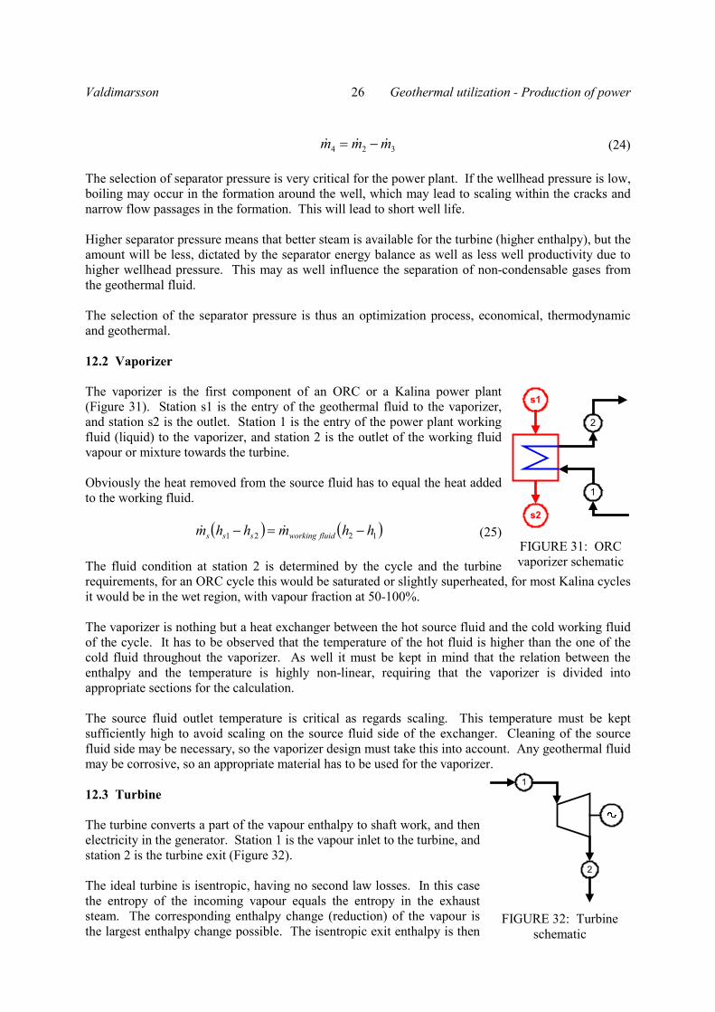
(24) The selection of separator pressure is very critical for the power plant. If the wellhead pressure is low, boiling may occur in the formation around the well, which may lead to scaling within the cracks and narrow flow passages in the formation. This will lead to short well life. Higher separator pressure means that better steam is available for the turbine (higher enthalpy), but the amount will be less, dictated by the separator energy balance as well as less well productivity due to higher wellhead pressure. This may as well influence the separation of non-condensable gases from the geothermal fluid. The selection of the separator pressure is thus an optimization process, economical, thermodynamic and geothermal. 12.2 Vaporizer The vaporizer is the first component of an ORC or a Kalina power plant (Figure 31). Station s1 is the entry of the geothermal fluid to the vaporizer, and station s2 is the outlet. Station 1 is the entry of the power plant working fluid (liquid) to the vaporizer, and station 2 is the outlet of the working fluid vapour or mixture towards the turbine. Obviously the heat removed from the source fluid has to equal the heat added to the working fluid.

(25) The fluid condition at station 2 is determined by the cycle and the turbine requirements, for an ORC cycle this would be saturated or slightly superheated, for most Kalina cycles it would be in the wet region, with vapour fraction at 50-100%. The vaporizer is nothing but a heat exchanger between the hot source fluid and the cold working fluid of the cycle. It has to be observed that the temperature of the hot fluid is higher than the one of the cold fluid throughout the vaporizer. As well it must be kept in mind that the relation between the enthalpy and the temperature is highly non-linear, requiring that the vaporizer is divided into appropriate sections for the calculation. The source fluid outlet temperature is critical as regards scaling. This temperature must be kept sufficiently high to avoid scaling on the source fluid side of the exchanger. Cleaning of the source fluid side may be necessary, so the vaporizer design must take this into account. Any geothermal fluid may be corrosive, so an appropriate material has to be used for the vaporizer. 12.3 Turbine The turbine converts a part of the vapour enthalpy to shaft work, and then electricity in the generator. Station 1 is the vapour inlet to the turbine, and station 2 is the turbine exit (Figure 32). The ideal turbine is isentropic, having no second law losses. In this case the entropy of the incoming vapour equals the entropy in the exhaust steam. The corresponding enthalpy change (reduction) of the vapour is the largest enthalpy change possible. The isentropic exit enthalpy is then

324 mmm −=

( ) ( )1221 hhmhhm fluidworkingsss −=−

FIGURE 31: ORC vaporizer schematic

FIGURE 32: Turbine schematic

s1

s2

1

2

1

2


the enthalpy at the same entropy as in the inlet and at the exit pressure, which is roughly the same as prevails in the condenser. (26) The turbine isentropic efficiency is given by the turbine manufacturer. This efficiency is the ratio between the real enthalpy change through the turbine to the largest possible (isentropic) enthalpy change. The real turbine exit enthalpy can then be calculated:

(27) The work output of the turbine is then the real enthalpy change multiplied by the working fluid mass flow through the turbine.

(28) The expansion through the turbine may result in that the exit vapor is in the wet region, or that a fraction of the mass flow is liquid. This can be very harmful for the turbine, resulting in erosion and blade damage. The Kalina cycle uses a mixture of ammonia and water, so that the droplets created in the turbine are electrically conductive. It is the meaning of the writer that this conductivity is the reason for the corrosion encountered in the turbine in Husavik, Iceland. This corrosion has been avoided by the usage of non-magnetic titanium for the turbine rotor. Many of the working fluids for the ORC cycle are retrograde, which means in this context that the exit vapour is superheated. The heat removal in the condenser will then partly be “de-superheat”, heat transfer out of the vapour at temperature higher than the final condensing temperature. Ammonia-water mixture is not retrograde, but as the condensation will occur at a variable temperature, the heat removal process is very similar to that of the retrograde fluids. 12.4 Recuperator The recuperator is a heat exchanger between the hot exit vapour from the turbine and the condenser. It is a de-superheater in the ORC cycle, transferring heat from the turbine exit vapour to the condensate from the condenser. Station 1 is the turbine exit vapour, station 2 is the recuperator outlet towards the condenser, station 3 is the inlet of the condensate from the condenser, and station 4 is the pre-heated feed to the vaporizer (Figure 33). The heat removed from the turbine exhaust vapour is equal the heat added to condensate:

(29) The mass flow is the same on both sides of the recuperator. The hot fluid from the turbine is on the hot side, will be condensed in the condenser and then pumped right away through the cold side of the recuperator towards the vaporizer.

( )21,2 , pshh s =

( )sis hhhh ,2112 −−= η

( )21 hhmW −=

( ) ( )3421 hhmhhm −=−

FIGURE 33: Recuperator schematic

1

2

4

3

Valdimarsson 28 Geothermal utilization - Production of power It has to be observed that the temperature of the hot fluid is higher than the one of the cold fluid throughout the recuperator. The fluid behaviour is usually close to linear, so it is normally not necessary to divide the recuperator into sections. The effect of recuperation on the cycle has been treated earlier in this text. 12.5 Condenser The condenser may be either water or air cooled. The calculations for the condenser are roughly the same in both cases, as the cooling fluid (air or water) is very close to linear. Station 1 is the working fluid coming from the recuperator (or turbine in the case of a non-recuperated cycle), shown in Figure 34. Station 2 is the condensed fluid, normally saturated liquid with little or no sub-cooling. Station c1 is the entry of the cooling fluid, station c2 the outlet. The condenser is nothing but a heat exchanger between the hot vapour from the recuperator/turbine and the cooling working fluid of the cycle. It has to be observed that the temperature of the hot fluid is higher than the one of the cold fluid throughout the condenser. As well it must be kept in mind that the relation between the enthalpy and the temperature is non-linear, requiring that the vaporizer is divided into appropriate sections for the calculation. This is especially valid for Kalina cycles, in the ORC cycle there is only a property change at the dew point, where de-superheat ends and condensation begins. 13. THERMOECONOMICS Thermoeconomics analyze the power generation economics from the exergetic viewpoint. A thorough treatment of thermoeconomics is found in Bejan et al (1996) and El-Sayed (2003). Thermoeconomics deal with the value of the energy within a plant, where heat and work conversion finds place. The analysis is based on exergy flows, and breaks the plant up into individual components, where each component can be analyzed separately. Each component will have one or more exergy input (feed) streams, and one or more output (product) exergy streams. A feed stream is either input to the plant, or is a product of a previous component. An output stream is either a product from the plant or a feed to the next component in the chain. Exergy loss due to irreversibilities will occur in all components of the power plant. This is the so-called exergy destruction, and the stream is termed exergy destruction stream for the subject component. In some components there will be a rejected exergy stream, which is of no further use in the process. This is the exergy loss, and exergy loss stream for the subject component. Figure 35 is a schematic which shows this relationship better.

FIGURE 34: Condenser schematic

FIGURE 35: Component exergy streams

c1

c2

1

2

Input exergy

DestructionLoss

Product 2

Product 1

Component


Anergy is assumed to have no value, as well as all exergy loss streams and destruction streams. The unitary exergy cost is calculated for each point in the energy conversion process, and cost streams are used to gain an overview over the economics of the power generation process. Each component will have three types of cost flows associated, the input exergy cost flow, the component investment cost flow, and the product exergy cost flow. A cost balance, equating the product cost flows (all having the same unitary exergy cost) to the sum of the input exergy cost flows and the component investment cost flow. The component has to be paid for and maintained. The associated cost is fixed, and is not dependent on the magnitude of the exergy streams entering and leaving the component. The investment cost flow is calculated as:

(30) Where ˙ = Dot above character denotes time derivative (rate) (1/s, 1/h); CI = Capital and investment (index); OM = Operation and maintenance (index); and Z = Fixed cost ($). The unitary exergy cost is important for the study of the component performance. Each kilowatthour of exergy entering and leaving the component carries cost (or has value), which can be compared to the cost of electricity. The exergy stream is then a product of the unitary exergy cost and the exergy flow:

(31)

where ˙ = Dot above character denotes time derivative (rate) (1/s, 1/h); e = Product, output, exit (index); C = Cost, value ($); c = Untiary (specific) cost, value ($/kWh); i = Feed, input (index); m = Mass (kg); q = Heat (index); W = Work (kJ, kWh); w = Work or power (index); X = Exergy (kJ, kWh); and x = Specific exergy (kJ/kg). The Sankey diagram shown in Figure 36 describes cost flow for a sample component graphically. There is no such thing as a free lunch. The cost flow of the products must be equal to the sum of all incoming cost flows, both those connected with exergy as well as the investment cost flow. This balance is written as:

(32)

CI OMZ Z Z= +

( )( )

i i i i i i

e e e e e e

w w

q q q

C c X c m x

C c X c m x

C c W

C c X

= =

= =

=

=

, , , ,e k w k q k i k ke i

C C C C Z+ = + +∑ ∑


FIGURE 36: Component cost (value) streams where ˙ = Dot above character denotes time derivative (rate) (1/s, 1/h); C = Cost, value ($); e = Product, output, exit (index); i = Feed, input (index); k = Number of component; q = Heat (index); w = Work or power (index); and Z = Investment cost ($). It is traditional in thermodynamics to consider heat flow as input and work flow as output. That is the reason for entering the heat cost flow as input and the work (power) cost flow as output. The product cost flow can now be solved from this equation, assuming that all previous components in the chain have already been solved. Equation 32 is now modified to include unitary cost values:

(33)

where ˙ = Dot above character denotes time derivative (rate) (1/s, 1/h); C = Cost, value ($); c = Unitary (specific) cost, value ($/kWh); e = Product, output, exit (index); i = Feed, input (index); k = Number of component; q = Heat (index); W = Work (kJ, kWh); w = Work or power (index); X = Exergy (kJ, kWh); and Z = Investment cost ($).

( ) ( ), , ,e e w k k q k q k i i kk ke i

c X c W c X c X Z+ = + +∑ ∑


Thermoeconomic optimization will not be treated further here, but this discipline has very powerful tools, enabling the designer to keep consistent economic quality in all components in the power production chain.

14. FEASIBILITY AND ECONOMICS Thermoeconomy is a very powerful tool to optimize individual plant components. One of the main benefits is that the thermoeconomic tools enable us to deign with consistent quality and performance for all of the installed components. This is a different question to the question if the plant is a good idea at all. A feasibility study should reveal that. In order to make a useable feasibility study, two main estimates have to be done:

a) Estimation of income; and b) Estimation of power plant cost

The income estimate cannot be done unless having a good process model at hand, taking into account the climatic conditions over the year, properties of the wells and geothermal fluid, as well as a thorough model of the plant internals. Such a model will then be able to yield estimates for the power produced by the generator, the power consumed by parasitic components such as circulation pumps and cooling tower and of course thermodynamic process data for the power plant cycle. The estimation of cost for the plant involves estimating the size of individual components and their price, in addition to installation and secondary cost. It is worth to keep in mind that roads, buildings, fire protection, environmental protection components, control systems, and even lockers and showers for the employees are also a part of the power plant cost. All this is small compared to the cost invested in the geothermal field, purchase or lease of land, concession fees, field research, and finally drilling of wells. In far too many cases this is considered sunk cost, and is not taken into the account when designing the power plant, with the result that the plant is optimal, assuming that all cost outside the plant is sunk and paid by space aliens. The cost estimate considering all the cost will yield a larger power plant, suboptimal if only the plant is considered, but giving a higher income and therefore a contribution to the amortization of the field cost. Renewable energy projects have typically very low variable cost if any at all. The plant has to be built and paid for in the beginning, and will after that produce power without much additional cost. Usually total cost will not be reduced if the plant is run on reduced power. The value of the parasitic power is sometimes complicating the calculations. The price of produced green energy from the power plant may be substantially higher than the market price on the grid due to green subventions. One possible way of simplifying this is to calculate a net present value for every kilowatt of parasitic power and simply add that to the plant investment cost. 14.1 The mathematics The three equations of engineering have to be fulfilled, always, everywhere:

a) Conservation of mass; b) Conservation of momentum; and c) Conservation of energy.

Valdimarsson 32 Geothermal utilization - Production of power The only way to make an estimation of the power produced and thus the income is to make a mathematical model of the power plant. The thermodynamic properties of the geothermal fluid and the plant working fluid have to be incorporated, and the model has to be built on the laws of thermodynamics. They are not subject to negotiation, they are absolute. The plant is then described in a large set of non-linear equations, which have to be solved. A mathematical environment called Engineering Equation Solver (EES) has been used by the author for this purpose. EES has thermodynamic properties of most of the relevant fluids built in, and is already an equation solver, as the name implies. Heavyweight software such as Aspen or Simulis is of course capable of such modelling, but is expensive and requires much training in order to be an effective tool. Matlab is a standard numerical environment today, but lacks thermodynamic properties. It is possible to integrate Matlab with properties programs made by the US National Institute of Standards (NIST), but this integration is not commercially available and requires in-depth knowledge of programming. Matlab is polished, tried and tested and has a huge user base. But Matlab is also a notorious “hard to learn, easy to use” program. 14.2 Degrees of freedom for the plant design A binary power plant has around 25-30 design parameters for the thermal design. Some of these parameters have values, which do not change much from case to case. Others are critical optimization parameters. All these parameters are dependent on the plant surroundings, the field parameters, and the market parameters. It is therefore absolutely critical to determine the plant input parameters correctly. The selection of all other parameter values is dependent on that. The score function for the plant operation is also critical. A common misunderstanding is to take some more or less well founded efficiency value and use that as the only criterion to determine if the plant is good or bad. A power plant is built to produce power as cost effectively as possible. Therefore it is a lot more sensible to base the power plant design on some specific power plant cost in $/kW, ensuring that both the cost model and the power plant model is reflecting the reality as closely as possible. Geothermal power production is simply a chain of components or processes from the inflow into the well all the way over to the power plant transformer station. The objective is to convert as much of the exergy found in the well inflow to sellable power, electricity or heat. And as typical with any chain, it will never be stronger than the weakest link. The power plant cold end and the associated cooling fluid supply is a part of this chain. The 25-30 design parameters that have to be selected define an optimization space with a dimension which is one higher that the number of parameters.. The optimization process has therefore a huge number of degrees of freedom, and there are not many general universally usable solutions available, which can give satisfactory performance. There is no way around a careful design and selection of all these design parameters. 15. GEOTHERMAL FIELD AND WELLS The well is one of the most expensive part of the power production system. The well will have production dependent on the wellhead pressure. The maximum flow will occur with wellhead pressure zero, and zero flow will yield the well closure pressure, which is again the maximum wellhead pressure. The well characteristic curve will be a deciding factor in the selection of the


separator pressure in the flash plants for higher enthalpy fields. Lower separator pressure, higher well flow, higher steam ratio from the separator, but lower quality steam. The lower the wellhead pressure, the lower in the well the boiling of the fluid will start, and finally boiling will occur in the formation, usually with horrible results. Scaling may occur in the formation, destroying the well. The field enthalpy is a major criterion for the power plant design, and will more or less determine which power plant type can be used. The fluid chemistry is another decisive factor. Scaling behaviour of the fluid usually demands a certain minimum geothermal fluid temperature to be held throughout the entire power plant. Corrosion may require certain materials or the use of additives. Non-condensable gas in the fluid may require gas extraction system with the associated parasitic loss. Therefore the power plant designer is bound by the fluid enthalpy and chemistry for his selection of the design parameters. To disregard the comments of the geochemist is a sure way to failure. From the viewpoint of thermoeconomics, the inflow to the well is free of charge, but when the fluid has reached the surface the exergy stream from the well has to carry the field development, drilling and well construction investment cost. 16. EXAMPLE OF COST CALCULATION Assume that the field development and well cost amounts to 5,000,000 € for each well. Two production wells are drilled and one re-injection well. The well production is 150 kg/s, and the well is low enthalpy, producing only liquid water. The environment is taken at 10°C, 1 bar pressure. Yearly capital cost and operation and maintenance are taken as 10% of investment. Utilization time is assumed 8,000 hours per year. Under these assumptions the well exergy flow can be calculated as well as the unitary exergy cost (Figure 37). These results show, that a substantial part of the final cost of electricity is already defined by the well. If we could buy an ideal lossless power plant at zero price, this would be the final cost of electricity.

REFERENCES

Bejan, A., Tsatsaronis, G., and Moran, M., 1996: Thermal design and optimization, J. Wiley, New York, NY, United States, 560 pp. Cengel, Y.A., and Boles, M.A., 2002: Thermodynamics: An engineering approach (4th edition). McGraw-Hill, 1056 pp. Dorj, P., 2005: Thermoeconomic analysis of a new geothermal utilization CHP plant in Tsetserleg, Mongolia. University of Iceland, MSc thesis, UNU-GTP, Iceland, report 2, 74 pp. Web: http://www. os.is/gogn/unu-gtp-report/UNU-GTP-2005-02.pdf

FIGURE 37: Unitary well exergy cost

110 120 130 140 150 160 170 180 190 2000,006

0,008

0,01

0,012

0,014

0,016

0,018

0,02

0,022

Geothermal fluid temperature [°C]

Spec

ific

cost

[€/k

Wh]

Valdimarsson 34 Geothermal utilization - Production of power El-Sayed, Y. M., 2003: Thermoeconomics of energy conversions. Pergamon Press, 276 pp. Kotas, T. J., 1985: The exergy method of thermal plant analysis. Butterworths, Academic Press, London, 296 pp. Szargut, J., Morris, D.R., Steward, F.R., 1988: Exergy analysis of thermal, chemical, and metallurgical processes. Springer-Verlag, Berlin, 400 pp. Thórólfsson, G., 2002: Bestun á nýtingu lághita jarðvarma til raforkuframleiðslu (Optimization of low temperature heat utilization for production of electricity). University of Iceland, Dept. of Mechancial Engineering, MSc thesis, 71 pp. Valdimarsson, P., 2002: Cogeneration of district heating water and electricity from a low temperature geothermal source. Proceedings of the 8th International Symposium on District Heating and Cooling, NEFP and the International Energy Agency, Trondheim, Norway. The following textbooks cover the material in this paper in more depth: DiPippo, R., 2008: Geothermal power plants: Principles, applications, case studies and environmental impact (2nd edition). Butterworth-Heinemann (Elsevier), Oxford, United Kingdom, 493 pp. Popovski, K., Andritsos, N., Fytikas, M., Sanner, B., Ungemach, P., and Valdimarsson, P., 2010: Geothermal energy. MAGA Macedonian Geothermal Association, Skopje, Republic of Macedonia.

geothermal utilization production power

Documents

power station

power plant internals

conversion of heat

independent production

maximum power figure

certain maximum power

integral of produced

geothermal source