gerhard link dissertation
TRANSCRIPT
A Finite Element Scheme for
Fluid–Solid–Acoustics Interactions
and its Application to
Human Phonation
Der Technischen Fakultat der
Universitat Erlangen-Nurnberg
zur Erlangung des Grades
DOKTOR - INGENIEUR
vorgelegt von
Gerhard Link
Erlangen, 2008

Als Dissertation genehmigt von
der Technischen Fakultat der
Universitat Erlangen-Nurnberg
Tag der Einreichung: 30. Juni 2008
Tag der Promotion: 17. Oktober 2008
Dekan: Prof. Dr.-Ing. habil. Johannes Huber
Berichterstatter: Prof. Dr. techn. Dr.-Ing. habil. Manfred Kaltenbacher
Prof. Dr.-Ing. habil. Kai Willner

Vorwort
Die vorliegende Arbeit entstand wahrend meiner Tatigkeit als wissenschaftlicher Mitar-beiter am Lehrstuhl fur Sensorik der Universitat Erlangen-Nurnberg. Die Arbeit wurdevon der Deutschen Forschungsgemeinschaft (DFG) im Rahmen der Forschergruppe 894und des Sonderforschungsbereichs 603 (TP C7) gefordert. Des Weiteren unterstutze dieBayerische Forschungsgemeinschaft (BFS) die Arbeit im Rahmen des Projektes Fluid-Struktur-Larm.
Mein herzlichster Dank gilt Herrn Prof. Dr. techn. Dr.-Ing. habil. Manfred Kaltenbacherfur die kontinuierliche Unterstutzung und den Ruckhalt wahrend der Durchfuhrung derArbeit sowie fur die Moglichkeit dieses spannende und breitgefacherte Thema bearbeitenzu konnen.
Bei Herrn Prof. Dr.-Ing. habil. Kai Willner bedanke ich mich ganz herzlich fur dieUbernahme des Zweitgutachtens und seine wertvollen fachlichen Anregungen.
Herrn Prof. Dr.-Ing. Reinhard Lerch danke ich fur seine Unterstutzung und das sehr an-genehme Arbeitsklima, das an seinem Lehrstuhl herrscht. Außerdem gilt mein Dank allenKollegen des Lehrstuhls fur Sensorik.
Herrn Prof. Dr. Dr. Ulrich Eysholdt und Herrn Prof. Dr.-Ing. Michael Dollinger danke ichfur die fruchtbare Kooperation bezuglich der menschlichen Phonation.
Des Weiteren danke ich Prof. Dr.-Ing. Michael Breuer, Dr.-Ing. Frank Schafer undDr.-Ing. Stefan Becker vom Lehrstuhl fur Stromungsmechanik fur die konstruktivenDiskussionen.
Mein Dank gilt auch Britta Hofmann fur die aufmerksame Durchsicht und Korrektur desManuskripts.
Besonders mochte ich mich bei meiner Familie fur den Ruckhalt bedanken auf den ichmich seit je her verlassen kann und bei meiner Freundin Eva Gehles fur Ihre liebevolleUnterstutzung.
iii


Contents
Notations and abbreviations vii
Abstract xiii
Kurzfassung xiv
1 Introduction 11.1 Multifield phenomenon . . . . . . . . . . . . . . . . . . . . . . . . . . . . . 11.2 Motivation for the medical application: human phonation . . . . . . . . . . 21.3 Models of human phonation . . . . . . . . . . . . . . . . . . . . . . . . . . 4
1.3.1 Self-sustained oscillation models . . . . . . . . . . . . . . . . . . . . 41.3.2 Aeroacoustic models . . . . . . . . . . . . . . . . . . . . . . . . . . 61.3.3 Motivation for improved computer models . . . . . . . . . . . . . . 71.3.4 Interim summary . . . . . . . . . . . . . . . . . . . . . . . . . . . . 8
1.4 Overview . . . . . . . . . . . . . . . . . . . . . . . . . . . . . . . . . . . . . 8
2 Physical fundamentals of fluid and solid mechanics 92.1 Nomenclature and reference systems . . . . . . . . . . . . . . . . . . . . . 92.2 Fluid mechanics . . . . . . . . . . . . . . . . . . . . . . . . . . . . . . . . . 16
2.2.1 Kinematics . . . . . . . . . . . . . . . . . . . . . . . . . . . . . . . 162.2.2 Kinetics . . . . . . . . . . . . . . . . . . . . . . . . . . . . . . . . . 162.2.3 Balance principles . . . . . . . . . . . . . . . . . . . . . . . . . . . . 182.2.4 The constitutive equation . . . . . . . . . . . . . . . . . . . . . . . 202.2.5 Governing partial differential equations . . . . . . . . . . . . . . . . 202.2.6 Initial and boundary conditions of fluid mechanics . . . . . . . . . . 232.2.7 Dimensionless numbers to characterize a flow . . . . . . . . . . . . 252.2.8 Turbulent flows . . . . . . . . . . . . . . . . . . . . . . . . . . . . . 26
2.3 Solid mechanics . . . . . . . . . . . . . . . . . . . . . . . . . . . . . . . . . 292.3.1 Kinematics . . . . . . . . . . . . . . . . . . . . . . . . . . . . . . . 302.3.2 Kinetics . . . . . . . . . . . . . . . . . . . . . . . . . . . . . . . . . 302.3.3 Balance principles . . . . . . . . . . . . . . . . . . . . . . . . . . . . 312.3.4 The constitutive equation . . . . . . . . . . . . . . . . . . . . . . . 312.3.5 Governing partial differential equations . . . . . . . . . . . . . . . . 342.3.6 Initial and boundary conditions of solid mechanics . . . . . . . . . . 34
2.4 Field interactions . . . . . . . . . . . . . . . . . . . . . . . . . . . . . . . . 342.4.1 Fluid-solid interaction . . . . . . . . . . . . . . . . . . . . . . . . . 352.4.2 Fluid-acoustics interaction – Aeroacoustics . . . . . . . . . . . . . . 372.4.3 Solid-acoustics interaction . . . . . . . . . . . . . . . . . . . . . . . 39
2.5 Interim summary . . . . . . . . . . . . . . . . . . . . . . . . . . . . . . . . 39
v

Contents
3 Numerical fundamentals 403.1 Computational fluid mechanics . . . . . . . . . . . . . . . . . . . . . . . . 41
3.1.1 Spatial discretization . . . . . . . . . . . . . . . . . . . . . . . . . . 423.1.2 Time discretization and linearization . . . . . . . . . . . . . . . . . 563.1.3 Validation examples . . . . . . . . . . . . . . . . . . . . . . . . . . 613.1.4 Interim summary on CFD . . . . . . . . . . . . . . . . . . . . . . . 73
3.2 Computational acoustics . . . . . . . . . . . . . . . . . . . . . . . . . . . . 733.3 Computational solid mechanics . . . . . . . . . . . . . . . . . . . . . . . . 73
3.3.1 Spatial discretization . . . . . . . . . . . . . . . . . . . . . . . . . . 733.3.2 Time discretization and linearization . . . . . . . . . . . . . . . . . 753.3.3 Geometric nonlinear validation example . . . . . . . . . . . . . . . 75
3.4 Fluid-solid-acoustics interaction . . . . . . . . . . . . . . . . . . . . . . . . 763.4.1 Coupling Strategies . . . . . . . . . . . . . . . . . . . . . . . . . . . 763.4.2 Fluid-solid interaction . . . . . . . . . . . . . . . . . . . . . . . . . 783.4.3 Fluid-acoustics coupling with Lighthill’s acoustic analogy . . . . . . 983.4.4 Solid-acoustics coupling . . . . . . . . . . . . . . . . . . . . . . . . 1033.4.5 Fluid-solid-acoustics algorithm . . . . . . . . . . . . . . . . . . . . . 105
4 Human phonation 1094.1 Medical principles . . . . . . . . . . . . . . . . . . . . . . . . . . . . . . . . 1094.2 Phonation model . . . . . . . . . . . . . . . . . . . . . . . . . . . . . . . . 1134.3 Vocal fold model . . . . . . . . . . . . . . . . . . . . . . . . . . . . . . . . 1144.4 Fluid mechanical validation of the 2d model with a 3d model . . . . . . . . 1154.5 Fluid-solid-acoustics coupled results . . . . . . . . . . . . . . . . . . . . . . 116
4.5.1 Development of the Coanda effect . . . . . . . . . . . . . . . . . . . 1164.5.2 Acoustic impact of the Coanda effect . . . . . . . . . . . . . . . . . 118
5 Summary and outlook 1235.1 Summary . . . . . . . . . . . . . . . . . . . . . . . . . . . . . . . . . . . . 1235.2 Outlook . . . . . . . . . . . . . . . . . . . . . . . . . . . . . . . . . . . . . 125
Bibliography 127
vi

Notations and abbreviations
In this thesis, scalars are represented by normal letters (b), Cartesian vectors are marked
with an arrow (~b), second order tensors are denoted by bold letters (b) and fourth ordertensors by bold letters in square brackets ([b]). Matrices are capital boldface Roman letters(B) and to denote the non-Cartesian vectors, small bold Roman letters (b) are used.
Abbreviations
FEM Finite element methodFDM Finite difference methodFVM Finite volume methodLBA Lattice Boltzmann automataCFD Computational fluid dynamicsLES Large eddy simulationPDE Partial differential equationIBVP Initial boundary value problemODE Ordinary Differential equationsALE Arbitrary Lagrangian EulerianLAS Linear algebraic equationBE Backward EulerCN Crank-NicholsonBDF2 2nd order backward differenceSUPG Streamline-upwind/Petrov-GalerkinPSPG Pressure-Stabilized/Petrov-GalerkinGLS Galerkin least squaresUSFEM Unusual stabilized finite element methodCBS Characteristic Based SplitLSFEM Least squares finite element methodFIC Finite increment calculusVMM Variational multiscale methodvf Vocal foldssub Subglottalsupra Supraglottal
Mathematical conventions∫Ω
dΩ Volume integral∫Γ
dΓ Surface integral∇ Gradient∇· Divergence
vii

Notations and abbreviations
∆ Laplacian∂/∂x Spatial partial derivative(·)i,x Partial derivative of component i to x
∂/∂t, ˙(·) Temporal partial derivative
(·) Temporal partial derivative of second orderD/Dt Substantial or total temporal derivative∂/∂~n Directional derivative with respect to ~n1 Identity matrix(·)T Transposed(·)−1 Invertedtr(·) TraceΠ() ProjectionΓfct Gamma function(·)|~x With respect to ~x
(·)| ~X With respect to ~X(·)|~χ With respect to ~χ
Differential operators
B Solid mechanics stiffness operatorL Fluid operatorLM Fluid momentum operatorLC Fluid continuity operatorLstab
M Stabilization operator for fluid momentumLstab
C Stabilization operator for fluid continuityA Navier-Stokes differential operatorMa Added mass operator
L Adjoint differential operators
Spaces
R3 Euclidean spaceL2 Space of square integrable functionsH1 Space of square integrable functions with square integrable derivativesV Functions space of velocityW Functions spaces of momentum test functionQ Functions spaces of pressure and continuity test function
Domains and Boundaries
Ω Simulation domainΓ Boundary of simulation domain~n Surface normalΩ Eulerian domainΩ0 Lagrangian domain
viii

Notations and abbreviations
Ωt ALE domainΩf Fluid domainΩs Solid domainΩa Acoustic domainΩEuler Fluid domain where no grid adaption is performedΩALE Fluid domain where grid adaption is performedΓfs Fluid-solid interfaceΓa Acoustic boundary
Symbols
t Time~x Spatial coordinate of the Eulerian frame~X Spatial coordinate of the Lagrangian frame~χ Spatial coordinate of the ALE framex, y, z Components of the spatial vectorL Spatial length~v Velocity~t Traction~fV Volume forceε Rate of deformation tensorσ Cauchy stress tensorτ Viscous stress tensorP Thermodynamic pressurep Kinematic pressure (p = P/ρ)ρ DensityT TemperatureR Universal gas constante Intrinsic energycv Isochor specific heat capacitycP Isobar specific heat capacityT TemperatureEtot Mass specific total energyq Conductive heat fluxk Thermal conductivityµ Dynamic viscosityν Kinematic viscosity (ν = µ/ρ)c Speed of soundKB Bulk modulus~I Sound intensityRe Reynolds numberMa Mach numberKn Knudson numberSt Strouhal numberEu Euler numberFr Froude number
ix

Notations and abbreviations
lk Kolmogorov length scaleτ turb Turbulence stress tensorτ sgs Turbulent subgrid scale stress tensora Turbulent anisotropy tensorIIa, IIa Second and third principle scalar invariant of akt Turbulent kinetic energyνt Turbulent viscosityεt Rate of turbulent dissipationCs Smagorinsky constant
~ffluid Fluid force~u Displacement~d Displacement at the fluid-solid interface (~d = ~u) on Γfs
F Deformation gradientE Green Lagrangian strain tensorε Cauchy strain tensorσ Cauchy stress tensorP 2nd Piola-Kirchhoff stress tensor[C] Elasticity matrixλs, µs Lame parametersE Elasticity modulusνs Poisson number[A], [B] Fractional matricesA Gruenwald coefficientsT Lighthill’s tensor~r Grid displacement
~w, q FEM test functionsτ Stabilization parameterK Finite Elementh Element sizeL Spatial lengthNi Interpolation functionΦ Complex potential function4t Time step sizeT Periodf Frequencyg Greens functionβ, γ Time integration parametersεfsa Fluid-solid convergence toleranceεg Grid adaption convergence tolerance
Indices
f Fluids Solid
x

Notations and abbreviations
a Acousticsg Gridc Convection0 Mean part of the acoustic decomposition
(·) Temporal mean value due to turbulence decomposition
(·)′ Fluctuating value due to turbulence decomposition
(·) Resolved scales of LES and VMM
(·)? Unresolved scales of LES and VMM
Matrices and Vectors
M Mass matrixK Stiffness matrixN Stiffness matrix originate from the velocity termG Gradient matrixD Damping matrixF Right hand side vectorv Vector of unknown velocitiesu Vector of unknown displacementsd Vector of interface displacements
d Vector of un-relaxed interface displacementsu Vector of predicted displacementsPa Vector of unknown sound pressurer Vector of unknown grid displacementvg Vector of unknown grid velocityag Vector of unknown grid acceleration
xi

Notations and abbreviations
Medical notations [41]
Glottis Air gap between the vocal folds - (Stimmritze)
Vocal fold One of Ferrein’s cords; the sharp edge of a fold of mucousmembrane overlaying the vocal ligament and stretching alongeither wall of the larynx from the angle between the laminaof the thyroid cartilage to the vocal process of the arytenoidcartilage; the vocal folds are the agents concerned in voiceproduction - (Stimmlippe)
Vocal chord Ligament of the vocal folds - (Stimmband)
Vocal muscle Shortens and relaxes the vocal folds - (Stimmmuskel)
Pharynx The throat; above the esophagus and the trachea;below the mouth and nasal tract - (Rachen)
Larynx The organ of voice production - (Kehlkopf)
Laryngectomy Surgical excision of the larynx - (Kehlkopfentnahme)
Esophagus Food pipe/digestive tract - (Speiserohre)
Trachea Air pipe - (Luftrohre)
Dysphonia Any disorder of phonation affecting voice qualityor ability to produce voice - (Dysphonie)
Epiglottis A leaf-shaped plate of elastic cartilage,covered with mucous membrane, at the root of the tongue,which serves as a diverter valve of the larynx - (Epiglottis)
Thyroid cartilage Cartilage of the larynx in form of a shield;protecting the inner larynx - (Schildknorpel)
Cricoid cartilage Ring shaped cartilage of the larynx - (Ringknorpel)
Arytenoid cartilage Cartilage of the larynx to adjust the vocal folds - (Stellknorpel)
Hyoid cartilage U-shaped bone at the base of the tongue that supportsthe tongue muscles - (Zungenbein)
Epithelium The purely cellular avascular layer covering all the free surfaces,cutaneous, mucous and serous, including the glands and otherstructures derived therefrom - (Epithel)
Anterior/ventral Denoting the front surface of the body - (zur Vorderseite)
Posterior/dorsal Denoting the back surface of the body - (zur Ruckseite)
Inferior/caudal Denoting the bottom of the body - (nach unten)
xii

Abstract
The focus of this thesis is on the development of a numerical scheme to capture the fluid-solid-acoustics coupling. As example application the human phonation process is chosen.Human phonation is a paradigm for multifield interactions and at the same time stillnot fully explored. Many investigations considering the fluid-solid interaction on the onehand and the fluid-acoustics interaction on the other hand have been undertaken. So far,no phonation model is based on the completely coupled system taking into account thefluid-solid-acoustics interaction. The several methods to establish the fluid-solid-acousticscoupling are selected because of their ability to represent the physical fields and theirinteractions most accurately. The finite element method is adopted to discretize the threephysical fields discussed: fluid and solid mechanics and acoustics. The mechanical and theacoustic fields are approximated with a standard Galerkin scheme and a residual-basedstabilization method is chosen for the fluid field. The fluid-solid and the solid-acousticsinteractions are based on continuum mechanics. The fluid-acoustics coupling is based onLighthill’s acoustic analogy. The developed steps of the scheme are verified through severalbenchmark problems. Novel steps of the computational scheme are the flow solver, thefluid-solid interaction, the fluid-acoustics and the fluid-solid-acoustics coupling. Finally, afluid-solid-acoustics benchmark is successfully simulated and presented. For the first timethe two sound generation mechanisms of fluid-solid interaction - the flow-induced and thevibrational-induced sound - are captured together. In the considered phonation model itis discovered that the hereby developing Coanda effect causes a broadband sound signal.The Coanda effect is the affinity of a fluid jet to attach to an adjacent surface, the pharynxwall in case of phonation. A broadband acoustic signal exists as well during hoarsenessand in the case of a substitute voice after a laryngectomy, leading to the hypothesis thatin these cases the Coanda effect is more severe in comparison to the healthy state. Thedeveloped scheme enabled to detect and justify this interconnection between the Coandaeffect and dysphonias. In case of human phonation this scheme opens up new possibilitiesto understand the phonation process more profoundly and to improve existing therapies.
Consequently, this study supplies an accurate fluid-solid-acoustics coupled scheme, whichrepresents each physical field as well as their interactions comprehensively and withoutany noteworthy simplifications. The simulation of human phonation is a first applicationsuccess.
xiii

Kurzfassung
Das Ziel dieser Arbeit ist die Entwicklung eines numerischen Verfahrens, das Fluid-Struktur-Akustik-Wechselwirkungen vollstandig abbildet. Als Anwendungsbeispiel wirddie menschliche Stimmbildung gewahlt, weil dies ein Musterbeispiel fur Mehrfeld-Wechselwirkungen ist und gleichzeitig noch Forschungsbedarf besteht. Viele Untersuchun-gen betrachteten entweder die Fluid-Struktur-Wechselwirkung oder die Fluid-Akustik-Kopplung. Bislang wurde die Fluid-Struktur-Akustik-Wechselwirkung noch in keinemPhonationsmodell berucksichtigt. Die einzelnen Methoden des Fluid-Struktur-Akustik-Verfahrens werden dahingehend ausgewahlt, dass sowohl die physikalischen Felder als auchderen Wechselwirkungen so genau wie moglich erfasst werden. Alle drei betrachteten physi-kalischen Felder - die Stromungsmechanik, die Strukturmechanik und die Akustik - werdenmit der Finite-Elemente-Methode diskretisiert. Das mechanische und das akustische Feldwerden mit der Standard-Galerkin-Methode approximiert und das stromungsmechanischeFeld mit einer residuenbasierten stabilisierten Methode. Mittels kontinuumsmechanischerBeziehungen wird die Fluid-Struktur- und die Struktur-Akustik-Wechselwirkung realisiert.Die Fluid-Akustik-Kopplung basiert auf der akustischen Analogie von Lighthill. Die ent-wickelten Abschnitte des Verfahrens werden mit zahlreichen Referenzbeispielen validiert.Neue Schritte des numerischen Verfahrens sind der Stromungsloser, die Fluid-Struktur-Interaktion, die Fluid-Akustik- und die Fluid-Struktur-Akustik-Kopplung. Schließlich wirdein erstes Fluid-Struktur-Akustik-Referenzbeispiel im Rahmen dieser Arbeit erfolgreich si-muliert und vorgestellt. Erstmals konnen die beiden Schallentstehungsmechanismen vonFluid-Struktur-Wechselwirkungen - der stromungsinduzierte und der schwingungsinduzier-te Schall - gemeinsam abgebildet werden. Im entwickelten Phonationsmodell wird fest-gestellt, dass der hierbei auftretende Coanda-Effekt zu einem breitbandigen Schallsignalfuhrt. Der Coanda-Effekt beschreibt das Bestreben eines Fluid-Strahls sich an eine be-nachbarte Flache, im Falle der Phonation die Rachenwand, anzunahern. Ein breitbandigesakustisches Signal existiert ebenfalls bei Ersatzstimmen nach einer Kehlkopfentnahme undbei Heiserkeit. Dies fuhrt zu der Hypothese, dass in diesen Fallen der Coanda-Effekt starkerausgepragt ist als im gesunden Zustand. Erst das entwickelte Verfahren ermoglichte die Er-kennung und Begrundung dieser Querbeziehung zwischen dem Coanda-Effekt und Dyspho-nien. Fur den Forschungsbereich der menschlichen Stimmbildung eroffnet dieses Verfahrensomit neue Moglichkeiten fur ein fundierteres Verstandnis der Stimmbildung sowie zurVerbesserung bestehender Behandlungsmethoden.
Im Ergebnis liefert diese Arbeit ein Fluid-Struktur-Akustik-Verfahren, das die einzelnenphysikalischen Felder sowie deren Wechselwirkungen umfassend und ohne nennenswerteVereinfachungen abbildet. Die Simulation der menschlichen Stimmbildung ist ein ersterAnwendungserfolg.
xiv

1 Introduction
Sound is an omnipresent physical phenomenon in daily life. Many senses of well-beingare connected with sounds, e.g. listening to a singer or to a musical instrument. Incase of human voice, it is the basis of communication and therefore a part of social life.Other examples within nature are the sound of the surf, the singing of a bird or the rustleof leaves in the wind. This list is arbitrarily expandable. On the other hand sound inthe form of noise is mostly undesirable and represents a pollution. Therefore, some soundsshould be preserved and others reduced. Despite its omnipresence, not all sound generationmechanisms are fully understood so far, often due to the existence of a physical multifieldproblem. The focus of this thesis is to develop a fluid-solid-acoustics coupled scheme, whichallows a better understanding of these three fields and their interactions. In a second step,the scheme is applied to simulate the human phonation process.
1.1 Multifield phenomenon
In many technical machineries, e.g. airplanes, trains, trucks and cars, the appearance ofnoise is a multifield phenomenon. All listed examples have relevance for urban areas. Thesound radiation of an airplane during start and departure represents an important factorfor the people living nearby. An airplane can generate noise by the turbo-jet engines,the flaps, the high buoyant equipment and the landing gears. Furthermore, the wheel-railcontact and flow around the pantograph are crucial noise producing mechanisms of trains.In the case of road vehicles, the wheel-roadway contact, the streamnoise and the noiseinduced by the engine are important emitters.
Within all listed examples fluid-solid interactions are present. The composition of theoverall radiated noise changes, depending on the velocity of the respective vehicle. It istherefore necessary to understand all noise generation mechanisms exactly in order to de-velop primary noise reduction, which in general makes more sense from an economicalpoint of view than to install secondary noise insulation. Fluid-solid-acoustics computa-tional schemes can make a significant contribution to this area.
There are many additional biological and medical problems in which multiple interactingfields are present. The human phonation process is an example for a fluid-solid-acousticsinteraction. The blood flow through veins and the blood flow induced by heart contractionare examples of fluid-solid interaction.
In a multifield phenomenon the interaction of the physical fields plays a crucial role.The focus of this thesis lies in the continuum mechanical fields: fluid and solid mechanicsand acoustics. Their relationship is sketched in Fig. 1.1. Fluid forces act thereby on aneighboring solid, which is deformed and thereby influences the velocity of the adheringfluid particles. Due to the solid deformation, the fluid domain changes and has to beadapted. The fluid-acoustics interaction is described by Lighthill’s acoustic analogy andthe solid-acoustics coupling by claiming coincident surface acceleration. Fig. 1.1 shows the
1

1 Introduction
Figure 1.1: Modeling of fluid-solid-acoustics interaction
approaches chosen in the mathematical modeling of the fields and their discretization. Thefluid field is modeled therein with the incompressible unsteady Navier-Stokes equations.The solid field is described by the geometric nonlinear Navier equations. The acousticsound propagation considered herein is assumed to be linear and therefore captured by thewave equation. The finite element method (FEM) is applied for all three physical fields asdiscretization method. The mechanical and acoustic fields are discretized with a standardGalerkin scheme and the fluid field with a residual-based stabilization approach.
The aim to treat multifield problems numerically is still a growing area of research andonly few publications exist providing an overview. Kaltenbacher’s book [91] represents themost comprehensive contribution. Therein the mechanical, the electro-magnetic and theacoustic fields are tackled as well as the following interactions: solid-acoustics, electro-magnetics, electro-magnetics-solid, electro-magnetics-solid-acoustics and fluid-acoustics.
The fluid-solid interaction is treated within the dissertation of Wall [146] and by Tez-duyar [134], Forster [57], Hubner [80], Dettmer and Peric [40]. Commercial codes, whichare able to resolve the fluid-solid interaction can be purchased, e.g. STAR-CCM+ [7], CFX[4]/ANSYS[3], ADINA [2] and FLUENT [6]/ABAQUS [1].
1.2 Motivation for the medical application: humanphonation
If the phonation process is disturbed due to a disease, as e.g. laryngeal cancer, communica-tion is strongly affected. It is therefore necessary to enhance therapies in order to minimizeaffliction caused by diseases. There are different approaches to improve existent therapies.Field studies of different physical quantities, like sound pressure, vocal fold displacements,
2
1.2 Motivation for the medical application: human phonation
Author Year Dimension fluid-solid fluid-acoustics
Ishizaka et al. [87] 1972 multi-mass + –
Alipour et al. [8] 2000 2d plane – –
de Vries et al. [36] 2002 2d plane + –
Zhao et al. [155] 2002 2d axi – Direct & Analogy
Sidlof [143] 2007 2d plane/multi-mass + –
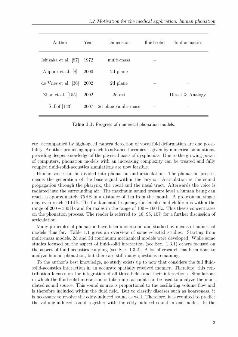
Table 1.1: Progress of numerical phonation models.
etc. accompanied by high-speed camera detection of vocal fold deformation are one possi-bility. Another promising approach to advance therapies is given by numerical simulations,providing deeper knowledge of the physical basis of dysphonias. Due to the growing powerof computers, phonation models with an increasing complexity can be treated and fullycoupled fluid-solid-acoustics simulations are now feasible.
Human voice can be divided into phonation and articulation. The phonation processmeans the generation of the base signal within the larynx. Articulation is the soundpropagation through the pharynx, the vocal and the nasal tract. Afterwards the voice isradiated into the surrounding air. The maximum sound pressure level a human being canreach is approximately 75 dB in a distance of 1 m from the mouth. A professional singermay even reach 110 dB. The fundamental frequency for females and children is within therange of 200− 300 Hz and for males in the range of 100− 160 Hz. This thesis concentrateson the phonation process. The reader is referred to [16, 95, 107] for a further discussion ofarticulation.
Many principles of phonation have been understood and studied by means of numericalmodels thus far. Table 1.1 gives an overview of some selected studies. Starting frommulti-mass models, 2d and 3d continuum mechanical models were developed. While somestudies focused on the aspect of fluid-solid interaction (see Sec. 1.3.1) others focused onthe aspect of fluid-acoustics coupling (see Sec. 1.3.2). A lot of research has been done toanalyze human phonation, but there are still many questions remaining.
To the author’s best knowledge, no study exists up to now that considers the full fluid-solid-acoustics interaction in an accurate spatially resolved manner. Therefore, this con-tribution focuses on the integration of all three fields and their interactions. Simulationsin which the fluid-solid interaction is taken into account can be used to analyze the mod-ulated sound source. This sound source is proportional to the oscillating volume flow andis therefore included within the fluid field. But to classify diseases such as hoarseness, itis necessary to resolve the eddy-induced sound as well. Therefore, it is required to predictthe volume-induced sound together with the eddy-induced sound in one model. In the
3

1 Introduction
present dissertation an enhanced approach for the fully coupled simulation is developed.The numerical model is implemented within the multifield finite element code CFS++ [93].
1.3 Models of human phonation
Textbooks on the subject of the principles of voice production are the two books of Titze[136, 137]. The current approaches of phonation analysis can be subdivided into two keyaspects, the self-sustained vocal fold oscillation and the aeroacoustics of human phonation.The self-sustained oscillation process is characterized by fluid-solid interaction. Studieson the volume-induced source of human phonation can be performed with such models.However, the volume-induced source is not the only acoustic source that exists withinhuman phonation. Hence, further investigations were performed to clarify the aeroacousticsources and their contribution to the overall sound of human phonation. A literature reviewon the state-of-the-art of numerical models to simulate self-sustained oscillation and theaeroacoustics of human phonation is given in the following.
1.3.1 Self-sustained oscillation models
Self-sustained oscillation models comprise a mechanical model representing both vocalfolds and a fluid mechanical model representing the air stream. The aeroacoustic aspect,which concerns the flow-induced sound, is neglected within this model. Furthermore,the approaches of self-sustained oscillation can be divided into multi-mass models andcontinuum mechanical models.
Multi-mass models
One of the most popular simulation models was developed by Ishizaka and Flanagan [87].They used a two-mass damper spring system to model the vocal folds coupled with theBernoulli equation representing the fluid field. It was the first simulation model thatsucceeded in reproducing self-sustained oscillation.
A general drawback of a multi-mass model to simulate human phonation is that sev-eral mass, damping, and stiffness parameters have to be determined. In the study ofde Vries et al. [37] this was done by a 3d simulation of the solid mechanics employingFEM.
Recently, a promising estimation scheme for the mass, the damping and the stiffnessparameters have been proposed by Dollinger et al. [42] and Wurzbacher et al. [150] basedon high-speed camera recordings of the vocal folds and an inverse optimization.
In the year 2002, results of a multi-mass model in combination with the Bernoulli equa-tion were published by Titze [138]. Therein the effect of cricothyropid and thyroarytenoidmuscles on the principle voice variables like the fundamental frequency, were investigated.
A first step towards the more advanced and computational costly continuum mechanicalmodels described in the next section is the semi-continuum model proposed by LaMar et al.[97]. They employed a modified quasi one-dimensional Euler system to model the airflow.It is semi-continuous, because the flow quantities of the air stream are spatial resolved,while the vocal folds are approximated by two discrete masses. This exhibits a higheraccuracy than the Bernoulli equation and successfully reproduced the double peaks of the
4

1.3 Models of human phonation
driving sub-glottal pressure at the opening and closing phase. It is simpler compared tomodels based on the Navier-Stokes equations, but has the shortcoming that the velocitydistribution cannot be predicted very accurately, as velocity variations in lateral-directionare neglected. However, an accurate resolved velocity distribution is the key to accurateaeroacoustic investigations [100].
A more recent study based on the approach of Ishizaka and Flanagan was carried out byChan et al. [26]. Their analytically based fluid-solid coupled model employs a multi-masssystem and the Bernoulli equation. They studied the effect of mechanical, geometric andacoustic properties on the phonation threshold pressure (PTP). The model predicts thatthe PTP increases with viscous shear but decreases with vocal tract inertia. They alsoperformed a validation by utilizing an experimental model.
Besides the mechanical parameters, the flow condition has to be modeled as well. There-fore the flow separation point is of particular importance in order to estimate the trans-glottal pressure loss. It can be used to model the resulting pressure drop along the glottis,which has a significant influence on the resulting vocal fold vibration. Decker et al. [38]compared three different methods to predict the flow separation point with the resultsgiven by a 2d Navier-Stokes solver. According to their studies the methods can yield poorflow separation point estimations, especially for a small glottis width.
Continuum mechanical models
In comparison with the multi-mass models described before, the continuum mechanicalmodels have the advantage of mathematically modeling the vibrations of the vocal folds inthe whole domain by partial differential equations. This mathematical modeling approachimplies a higher accuracy but is accompanied by higher computational costs.
Alipour et al. [8] published a finite element model of vocal fold vibration and Berry et al.[14] studied with it the effect of vocal fold scarring on phonation, such as the fundamentalfrequency. In their 2d model the mechanical field was discretized with finite elementsand the fluid forces were modeled, based on the Bernoulli equation. A Rayleigh dampingmodel was applied for the mechanical field to take viscosity into account. The vocalfolds were assumed to be geometrically linear, vocal fold symmetry was applied and ahemilarynx model was used. They concluded that increasing viscoelasticity increases themain frequency as well as the PTP and decreases the acoustic intensity.
As the main computing time is spent by solving the fluid mechanical field, it is of specialinterest whether simplified models like the Bernoulli equation can be used. A comparisonbetween a Bernoulli and a 2d Navier-Stokes solver was discussed by de Vries et al. [36]with a hemilarynx model. De Vries et al. [36] summarized, that the PTP based on aNavier-Stokes approach was more realistic than based on the Bernoulli equation. De Vriesdiscovered that with the Navier-Stokes equation the fundamental frequency increases withincreasing sub-glottal pressure.
Thomson et al. [135] used a hemilarynx continuum mechanical model. The main focusof their research was to clarify the reason for self-sustained vocal fold oscillation. Theydetected a cyclic variation of the glottis profile from a convergent to a divergent shape asthe key factor for self-sustained vocal fold oscillation. This leads to a temporary asymmetryin the average wall pressure.
Tao et al. [131] combined a collision model with fluid-solid interaction within a contin-uum framework. A strongly coupled fluid-solid algorithm was applied therein to tackle the
5

1 Introduction
interactions. Tao et al. also used a hemilarynx model.Hofmans et al. [78] discussed the legitimacy of hemilarynx models because it represents
a wide spread simplification of human phonation. Based on an experimental setup of anin-vitro larynx model, the symmetry assumption was investigated, considering the fluidmechanical field. The mechanical field as well as the fluid-solid interaction were neglectedfor that reason. The experimental model under investigation was a channel with a rigidorifice through which air was guided. Hofmans et al. [78] recommended the usage ofhemilarynx models, because the Coanda effect and turbulence takes too long to develop.In phonation situations with closing vocal folds, this argument may hold due to the factthat the flow has only one cycle to develop completely after a glottis opening. Nevertheless,there also exist phonation situations in which the vocal folds do not get in touch with eachother (i.e. glottis closure insufficience) [119]. The too short span of time is not an argumentagainst the occurrence of the Coanda effect for these contactless situations. From the fluidmechanical experimental setup of Hofmans et al. [78] it is not clear which impact thefluid-solid interaction has on the development of the Coanda effect. In phonation thisinteraction always exists. Therefore, the development of the Coanda effect needs to beinvestigated further.
Full 3d coupled simulations to analyze human phonation are very challenging for currentcomputing resources. Rosa et al. [120] presented a 3d fluid-solid coupled method whichwas based on FEM. Therein, the contact of the vocal folds was also taken into account. Themesh, consisting of 2600 tetrahedron finite elements for the fluid field and 3000 tetrahedronfinite elements for the mechanical field, was very coarse.
Gunter [69, 70] described a model which is capable of simulating the nonlinear collisionof the vocal folds with a continuum mechanical approach. She studied stress distributionas well, as this is a possible risk factor for pathological developments. The model wasbased on a 3d linear elastic finite element representation of a single vocal fold with arigid midplane surface. The fluid field was eliminated and quasi-static pressure boundaryconditions were applied.
Alipour et al. [9] presented a different approach, based on the finite volume methodto model the air stream. They examined a 2d hemilarynx model. The oscillation wasprovided by a sinusoidal varying inflow profile. The interaction between fluid and solidwas neglected and, therefore, the velocity boundary conditions are independent of thevocal fold motion. Their main concern was the flow separation point, which may also bedependent on fluid-solid interaction.
1.3.2 Aeroacoustic models
Besides the investigations considering vocal fold self oscillation, a growing interest in theaeroacoustic aspects of phonation can be observed. Zhao et al. [154, 155] and Zhang et al.[152] discussed the basics of acoustic sources generated by fluid flows. They describedthe aerodynamic generation of sound in a rigid pipe under forced vibration. They ne-glected fluid-solid interaction for simplicity and focused on fluid-acoustics coupling basedon Lighthill’s acoustic analogy, which was solved with an integral method - the so-calledFfowcs Williams-Hawkins (FWH) method [147]. They performed 2d axisymmetric fluidsimulations with a finite difference scheme. Due to the restriction of axisymmetry theCoanda effect could not be accounted for. The results based on the FWH method werein good compliance with the results based on direct numerical simulations, which solve
6

1.3 Models of human phonation
the compressible Navier-Stokes equations. A weak influence of the orifice geometry onthe sound amplitude was detected. Due to the fact that the orifice geometry has a highinfluence on the self-sustained oscillation, the geometry dependency on the fluid-inducedsound generation has to be considered within a fluid-solid interaction algorithm.
Zhang et al. [153] also did experimental investigations. Air was guided through rigidglottis-like orifices and the broadband noise of a jet was quantified through measuredsound pressure spectra. They studied the effects of the orifice geometry on broadbandsound generation. Altogether, they studied three different orifice geometries: a straight, adivergent and a convergent orifice. It was detected that for the straight and the convergentorifice the quadrupole is the dominant sound source. A tonal sound at low flow rates and abroadband sound at high flow rates were identified for the divergent orifice. In addition, theorifice geometry had significant influence on the sound. However, it is not clear whether theobserved mechanisms persist in the case of an unsteady flow under fluid-solid interaction,as it is the case in phonation.
Complementary to the above studies, Krane [96] researched the aeroacoustic phonationprocess. He considered unvoiced speech production with a theoretical approach. The focusof his paper was on describing the fluid-induced sound in phonation. The acoustic sourceswere computed based on a prescribed jet profile, in which the vorticity distribution wasmodeled by a formal expression. The discussed acoustic source distributions is based onan axisymmetric model of the vocal tract. He suggested describing the jet as a train ofvortex rings. Krane [96] computed the acoustic sources for a single vortex ring and builtup the overall acoustic sound of the pulsating jet by a convolution of vortex rings.
1.3.3 Motivation for improved computer models
Two conceptually different approaches are applied for the mechanical field of the vocalfold: the multi-mass and the continuum mechanical approach. The main advantage of amulti-mass model is its numerical simplicity. These models are still in use nowadays forthis reason. A critical point hereby is the correct choice of the parameters for masses,dampers and springs contained in the model. Furthermore, the approximation of the flowseparation point is a challenging task for this approach.
In modeling the air flow during phonation, there exist two main conceptually differentapproaches. These are given by the Navier-Stokes equations and the Bernoulli equation.Decker and Thomson [38] summarize that, for the simulation of self-sustained oscillation,reduced models based on energy equations, like the Bernoulli equation, are appropriate.However, aeroacoustic investigations based on flow results of the Bernoulli equation arevery restricted. The spatial velocity distribution is thereby given very roughly in formof cross-section velocities, allowing resolution of only the stream-wise velocity gradient.Therefore, simulations based on the Bernoulli equation are not adequate for aeroacousticinvestigations. For this reason, the author proposes to apply a Navier-Stokes solver torepresent the fluid mechanical field of phonation.
Another wide spread simplification of human phonation models represents the appli-cation of vocal fold symmetry. Hereby, hemilarynx models are used, which predict asymmetric behavior of the two vocal folds and thus also a symmetric shape of the air jet.Hemilarynx models have the advantage of reduced computational time because the dis-cretized domain is only half the size of the complete one. However, hemilarynx models donot contain the complete physics of human phonation. The key effect of asymmetry is the
7

1 Introduction
so-called Coanda effect. One example which shows this effect is the study of Shinwari et al.[130]. They presented results of a fluid mechanical experiment model of the larynx. Themodel represented a rigid larynx without fluid-solid interaction. They studied intra glottalpressure and jet flow for a divergent glottis and detected asymmetrical flow conditions.The air jet tended to touch a wall - this process is called Coanda effect. They suggestedtaking the Coanda effect into account for aeroacoustic investigation. The Coanda effectwas also detected to influence the sound production [46].
Another simplification is the assumption of 2d behavior. Especially for the flow, thisseems to be a strong simplification. On the other hand 3d simulations are restricted dueto computational costs. This is also the reason for this thesis to include 2d investigations.But in order to verify the 2d fluid results, a 3d fluid mechanical simulation was performedin addition.
1.3.4 Interim summary
As shown in this chapter, many investigations considering the fluid-solid interaction onthe one hand and the fluid-acoustics interaction on the other hand have been undertaken.So far, no contribution is based on the completely coupled system taking into account thefluid-solid-acoustics interaction. Especially for the investigation of the Coanda effect onphonation, a fully coupled fluid-solid-acoustics model is necessary. Therefore, the fluid-solid-acoustics interaction represents the main challenge for improved simulation modelsof human phonation.
1.4 Overview
The dissertation is organized as follows. In chapter 2, the principle of the physical fields andtheir interaction is summarized. In chapter 3, the numerical methods and, in chapter 4,fluid-solid-acoustics simulations of human phonation are presented. The thesis closes witha summary and an outlook in chapter 5.
8

2 Physical fundamentals of fluid andsolid mechanics
In this chapter the underlying physical principles of fluid and solid mechanics are sub-sumed. The theoretical framework is thereby given by continuum mechanics. The wavepropagation in fluids is derived based on fluid mechanical relations and afterwards treatedas a separate physical field: the acoustic field. Initial boundary value problems (IBVPs) arederived for all three considered physical fields - the fluid mechanical, the acoustic and thesolid mechanical field. The discretization of these IBVPs is the topic of the next chapter.
The composition of continuum mechanical relations yields an IBVP reproducing the phe-nomena of the respective physical field, see Fig. 2.1. Each IBVP consists of a set of partial
Figure 2.1: Continuum mechanical relations to derive a closed mathematical model.
differential equations (PDEs) equipped with sufficient initial and boundary conditions, sothat a mathematically well-posed problem is obtained.
2.1 Nomenclature and reference systems
In continuum mechanics the bodies are considered to be composed of a continuously dis-tributed material. In general, however, every body is known to be composed of atoms andmolecules which in turn consist of protons, neutrons and electrons, consisting of quarks andstrings. Hence, from a microscopical point of view each body is not continuous. Despitethat complex microscopic conglomerate, most bodies can be assumed to be continuous forthe purpose of analyzing most technical and biological problems because the characteristicmacro- and microscopic length scale differs with several orders. At the macroscopic scale,field quantities like density or temperature are used to associate the internal state. Ameasure of the scale ratio is given with the Knudsen number Kn:
Kn :=λ
L.
The Knudsen number is the ratio of the mean free path of molecules λ to the characteristicgeometrical measure L. The material can be supposed to be continuously distributed forsmall Knudsen numbers Kn 1. Almost every technical and biological application allowsthe application of the continuum approach. Even the smallest turbulent eddy possesses
9

2 Physical fundamentals of fluid and solid mechanics
a characteristic length scale of approximately three orders of magnitude larger than thecharacteristic molecular scale [44, 115]. To analyze durability, dynamics or sound genera-tion, the continuum mechanical theory is appropriate. The question concerning differentscales is quite fundamental. E.g. whether a certain body is considered as a solid or a fluiddepends on the characteristic time scale. In a geological time scale continents can drift andmountains can flow. In a human time scale both are solid. Bodies involved in biologicalor technical processes generally possess fluid as well as solid properties. It is a questionof time scale which effect dominates and if one of them can be neglected or not. Withinthe solid mechanical chapter a promising fractional constitutive equation which combinesfluid and solid properties is described. Different scales also exist within fluid mechan-ics. Sound propagation and fluid flows e.g. possess scale disparity. Turbulent flows caneven possess large scale disparity. In numerical methods the scale disparity is utilized e.g.to develop turbulence models in fluid mechanics. Large-eddy simulations (LES) assumemultiple scales within the solution and treat different scales with different mathematicalmodels. The recently upcoming variational multiscale approaches basically do the same,using different formulations for different scales. Scale difference is an omnipresent propertyin physics.
The continuum mechanical relations can be split into two groups, see Fig. 2.1: the ma-terial dependent and the material independent group. Kinematics, kinetics and balanceprinciples belong to the material independent group. All material independent relationsare identical for fluids and solids. Material dependency is introduced by the constitutiveequation. The derivation of the field PDEs demands the composition of kinematic, kinetic,balances and constitutive relations. Kinematics covers the geometric aspect of a deforma-tion. Its task is to provide measures for a certain deformation state as e.g. the deformationgradient tensor or measures for the strain. The choice of a reference system is therefore akinematic topic. The task of kinetics is to classify forces - both outer and inner forces aswell as the relation between them. Hereby measures of load states are provided, like stressvectors and tensors. The balance principles capture prevailing principles like the con-servation of mass, momentum and energy. The constitutive equation finally introducesthe material dependency by providing a relation between kinematic and kinetic quantities.The difference between fluid and solid mechanics is therefore captured in the constitutiveequation. In the case of solid mechanics, the principle unknown variable is displacement.In fluid mechanics, the principle unknown variable is velocity because of the fundamentalproperty of a fluid being a substance without a fixed shape. The molecules within a fluidcan move freely past one another. Thus, fluids take on the shape of their container. Ina fluid a certain shape change does not yield an inner stress as it is the case in a solid.A fluid experiences inner stress under the action of a velocity gradient. The constitutiveequation of a fluid therefore relates the stress to the rate of deformation gradient, whilefor a solid a relation between the stress and the deformation gradient is provided.
To introduce the continuum mechanical approach the frequently used nomenclature isdefined first. Afterwards three reference systems: the Lagrangian, the Eulerian and theArbitrary-Lagrange-Eulerian (ALE) systems are introduced and build the basis for mea-sures of the body motion. Related to these reference systems the Reynolds’ transporttheorem and the geometry conservation within the ALE systems are discussed. The gov-erning partial differential equations (PDEs) of the fluid, the acoustic and the solid field arederived with these basic relations. Thereby, the same subdivisions in material dependentand independent relations as shown in Fig. 2.1 are used.
10

2.1 Nomenclature and reference systems
Figure 2.2: A body B composed of particles <
(a) (b)
Figure 2.3: Domain and boundary definition: (a) field domains and interface boundary;(b) types of boundary conditions.
Nomenclature: At this stage the material reference system defined in the next chapteris applied. In order to derive the governing partial differential equations of the respectivefields the following terminology is introduced.
• Particles:Particles < already represent a macroscopic element. On the one hand a particle hasto be small enough to describe the deformation accurately and on the other handlarge enough to allow the application of the continuum approach. E.g. Fig. 2.2displays a fluid particle.
• Body:A body B consists of a set of particles <, see Fig. 2.2, and captures a certain regionin the Euclidean space R3.
• Configuration:A configuration of a body B is a unique map Φ : B → R3 of all its particles < in theEuclidean space R3.
The motion of a body B can now be prescribed as a time sequence of configurationsΦt : B → R3. The location of a particle ~X at time t is thereby ~x = Φt( ~X) = Φ( ~X, t). ~Xdenotes the initial particle location at t = 0.
In Fig. 2.3 domain and boundary terminologies are introduced to simplify further deriva-tion. The domains are denoted as Ωf , Ωs or Ωa whereas the subscript indicates the respec-tive field. The field interfaces are denoted by Γ equipped with subscripts of small letters
11

2 Physical fundamentals of fluid and solid mechanics
denoting the adjoint fields, e.g. Γfs denotes the fluid-solid interface. One letter is usedfor field boundaries without a neighboring field, e.g. Γa for the free acoustic boundary.So far, the nomenclature has only introduced information regarding the field interfaces.Speaking in terms of boundary condition types, the fluid-solid interaction, for example, isfor the fluid domain a Dirichlet boundary and for the solid domain a Neumann boundary.Therefore, fluid-solid interaction is also described as a Dirichlet-to-Neumann problem. Anadditional terminology is defined for discussions concerning the boundary condition type,see right hand side of Fig. 2.3. In this thesis only Dirichlet and Neumann boundary con-ditions are applied which are denoted by the capital letters D and N after a small letterdenoting the respective field. The following relations thereby hold for the solid boundary:
Γs = ΓsD ∪ ΓsN ∧ ΓsD ∩ ΓsN = ∅ .
In order to describe the body motion mathematically, an observer and a reference systemhas to be introduced.
Euler, Lagrange and ALE reference systems: Truesdell distinguishes altogether fourapproaches to describe the movement of a body, well known and most frequently appliedare [73]: the Lagrangian and the Eulerian approach. The difference between them is givenby the location of the observer, watching a certain body motion. The observer can also beunderstood as a reference system, which is in such a case the basis for motion measures.In the context of numerical simulations and especially in case of the herein applied FEM,the mesh can be understood as the reference system or as the observer. To highlight thisconnection between the reference system and the FEM mesh, the expressions Lagrangian,Eulerian and ALE-mesh are used.
The Lagrangian approach is a material based one, which means that the observer isfixed to moving particles. Solid mechanical problems are commonly formulated with theLagrangian approach. One advantage of the Lagrangian approach is that complex bound-ary conditions can be applied easily [13]. In the case of FEM a Lagrangian mesh getsdeformed together with the material particles and boundary nodes thereby remain at theboundary.
The Eulerian approach in contrast is field oriented. The observer is thereby fixed in spaceand watches the particles passing. The Eulerian approach discusses the temporal changeof a field function regarding a fixed point in space [10]. Most fluid mechanical problemsare formulated by the Eulerian approach [13]. One main advantage of the Eulerian meshis that the elements remain unchanged over time. Therefore large deformations can bedealt with easily. Under large deformations a Lagrangian mesh would become highlydistorted, yielding increasing numerical errors. Especially in fluid mechanical applicationsseveral fluid particles can undergo very high deformations. This would not appropriatelyrepresent the real physical process in a fluid. Fluid mechanical problems are commonlysimulated with an Eulerian reference system for that reason.
A challenge is now faced by a fluid domain with moving boundaries, which naturallyarises in fluid-solid interacting applications at the field-interface Γfs (Fig. 2.3). In order totackle fluid mechanics with moving boundaries and to combine the advantages of the La-grangian and the Eulerian approach, the Arbitrary-Lagrangian-Eulerian (ALE) approachis suggested [13, 43]. The ALE frame is a generalized reference system, the Lagrangianand the Eulerian systems can be derived from it. Besides the ALE approach, further
12

2.1 Nomenclature and reference systems
approaches are successfully applied to fluid flows on moving domains as well. E.g. thespace-time, the fictitious domain, the level set and the immersed boundary [111] methods.The most popular however, is the ALE description. Especially because of its flexibility,the ALE approach is applied in this thesis, to treat fluid flows on moving domains.
The basic idea of the ALE formulation is that the observer and the reference system canmove arbitrarily. In the context of fluid-solid interactions the movement of the referencesystem is not completely arbitrary. In that case the ALE reference system follows the fluiddomain deformation at the interacting boundary and arbitrary inside, so that the fluidelements are deformed as little as possible.
Fig. 2.4 shows the relation between the introduced reference systems. Generally, thesesystems move relative to each other, which is indicated by the mappings Φ, Ψ and Φ.~x, ~X and ~χ represent the spatial variables of the respective reference systems. The domains
Figure 2.4: Reference systems
are denoted accordingly: the Lagrangian domain Ω0, the Eulerian domain Ω and the ALEdomain Ωt. Each physical quantity, e.g. the scalar f , can be described in each referencesystem yielding different mathematical formulations. The mathematical formulation of fcan be transformed from the Lagrangian to the Eulerian system with the mapping Φ
f ∗∗( ~X, t) = f(Φ( ~X, t), t) = f(~x, t) or
f ∗∗ = f Φ .
Hereby ()∗∗ denotes that the mathematical formulation of f is based on the Lagrangianapproach. By applying the respective mapping the different mathematical formulationshave to yield a coincident result at a certain point in space
f(~x, t) = f ∗(~χ, t) = f ∗∗( ~X, t) .
The asterisk ()∗ and ()∗∗ denote that the mathematical formulation is in general different
in each system whereby ~x = Φ(~χ, t) and ~x = Φ( ~X, t)
f ∗ = f Φ = f (Φ Ψ−1) and f ∗∗ = f Φ .
The indices ()∗ and ()∗∗ are omitted from now on to simplify the equations, but it should bekept in mind that the functional form of a certain quantity is different in different referencesystems.
13

2 Physical fundamentals of fluid and solid mechanics
To formulate the balance principles the total time derivative is needed in order to takeinertia effects into account.Lagrange: The total time (substantial) derivative of the velocity ~v is given by the timederivative based on the material reference system
D~v
Dt=
∂~v
∂t
∣∣∣∣~X
. (2.1)
Euler: Based on the Eulerian system with the particle velocity ∂~x/∂t| ~X = ~v| ~X = ~v, thetotal time derivative is given by the chain rule
D~v
Dt
∣∣∣∣~X︸ ︷︷ ︸
Substantial acceleration
=∂~v
∂t
∣∣∣∣~x︸ ︷︷ ︸
Local acceleration
+ ~v∂~v
∂~x︸︷︷︸Convective acceleration
(2.2)
and is composed of a local change and a convective contribution of inertia.ALE: The total time derivative based on the ALE system can be derived accordingly andreads as
D~v
Dt
∣∣∣∣~X
=∂~v
∂t
∣∣∣∣~χ
+ (~v − ~vg)∂~v
∂~χ=
∂~v
∂t
∣∣∣∣~χ
+ ~vc∂~v
∂~χ. (2.3)
Hereby ~vg denotes the grid velocity and ~vc the convective velocity, whereby
~vc = ~v − ~vg . (2.4)
Reynolds’ transport theorem: The finite element method demands an integral formula-tion. To derive the integral form of the balance equations the rate of change of integrals ofscalar and vector functions has to be described, which is known as the Reynolds’ transporttheorem. The volume integral can change for two reasons: either the scalar or vector func-tions change or the volume changes. The following discussion is directed to scalar valuedfunctions. Vector valued functions are treated analogically. In the material configurationthe domain Ω0 does not change, but in the Eulerian and in the ALE configuration thevolume may change.Lagrange: In the material domain the time derivative can be moved inside the integral:
D
Dt
∫Ω0
f(~x, t) dΩ0 =
∫Ω0
∂f(~x, t)
∂t
∣∣∣∣~X
dΩ0 . (2.5)
Euler: In the spatial domain the change of the volume integral in time is composed of thechange of the scalar f and the fluxes across the surface:
D
Dt
∫Ω
f(~x, t) dΩ =
∫Ω
∂f(~x, t)
∂t
∣∣∣∣~x
dΩ +
∮Γ
f~v · ~n dΓ
=
∫Ω
(∂f(~x, t)
∂t
∣∣∣∣~x
+∇ · (f~v)
)dΩ . (2.6)
In the above formula the integral theorem of Gauss is applied to rewrite the surface integral.The same formulation can be obtained by transforming the integral to the material domain
14

2.1 Nomenclature and reference systems
and by moving the time derivative inside [10]. For an incompressible flow the Reynolds’transport theorem reduces to:
D
Dt
∫Ω
f(~x, t) dΩ =
∫Ω
(∂f(~x, t)
∂t
∣∣∣∣~x
+ ~v · ∇f(~x, t)
)dΩ . (2.7)
ALE: The Reynolds’ transport theorem of the ALE frame can be derived analogically andis finally given by:
D
Dt
∫Ωt
f(~x, t) dΩt =
∫Ωt
∂f(~x, t)
∂t
∣∣∣∣~χ
dΩt +
∮Γt
f~vc · ~n dΓt
=
∫Ωt
(∂f(~x, t)
∂t
∣∣∣∣~χ
+∇ · (f(~x, t)~vc)
)dΩt (2.8)
=
∫Ωt
(∂f(~x, t)
∂t
∣∣∣∣~χ
+ ~vc · ∇f(~x, t) + (∇ · ~vc)f(~x, t)
)dΩt .
Geometry conservation law: Numerical instabilities were observed in finite volume sim-ulations of fluids on moving grids. Demirdzic and M. Peric [39] showed that the gridvelocity ~vg has to be computed in such a way that the so-called space conservation law issatisfied to avoid instabilities. The terminology of space conservation and geometry conser-vation is identical. The reason for the instabilities is the accumulation of artificial sourceswhich destroy the mass conservation. The artificial source arises due to erroneous surfaceintegration [39]. Only a smaller time step size 4t decreases those sources.
The geometry conservation for a FEM discretization in an ALE mesh can be derived byconsidering the change of the ALE domain [55, 111]
D
Dt
∣∣∣∣~χ
∫Ωt
dΩt =
∫Ω0
∂Jt
∂t
∣∣∣∣~χ
dΩ0 =
∫Γt
~vg · ~n dΓt (2.9)
with the Jacobian determinant Jt
Jt = det
(∂~x
∂~χ
). (2.10)
The local form of (2.9) yields the geometry conservation law as
1
Jt
∂Jt
∂t
∣∣∣∣~χ
−∇ · ~vg = 0 . (2.11)
A FEM discretization for the convective formulation of fluid mechanics satisfies (2.11) assoon as an equivalent time discretization is applied to compute the grid velocity ~vg andthe fluid field ~v [56]. The grid velocity ~vg has to be approximated with the same order intime as the fluid mechanical quantities.
The following chapters proceed with detailed formulations for each field and their inter-actions.
15

2 Physical fundamentals of fluid and solid mechanics
2.2 Fluid mechanics
In this thesis the finite element code of the Department of Sensor Technology, CFS++ [93],is equipped with a fluid solver. The developed fluid solver can treat incompressible viscousflow of homogeneous isotropic fluids as described by the incompressible Navier-Stokesequations. In order to work out the relation to acoustics, the equations of compressibleflow are described as well in order to derive the wave equation. The wave equation is anappropriate mathematical formulation for linear acoustics. A complete description of fluidmechanics is beyond the scope of this thesis. Broad introduction to fluid mechanics ise.g. provided by Durst [44], Schlichting [128], Fletcher [53] and Herwig [75]. The reader isreferred to Pope [115], Davidson [35], Breuer [21], Rotta [122] and Hinze [77] for detailedinformation about turbulent flows.
2.2.1 Kinematics
The velocity field ~v(~x, t) of a body motion is of importance for fluids. A common way tovisualize the velocity field is given by path- and streamlines (see Fig. 2.5).Pathlines are the geometric locations of all space points of a single fluid particle duringa certain span of time.In contrast, a Streamline is connected to a single time step. Streamlines are lines withcoincident tangents as they exist in the current velocity field. In a stationary flow both
Figure 2.5: Path- and streamline to visualize a flow field.
lines are coincident. The fluid field is derived in an ALE description because of the fluid-solid interactions discussed in this thesis. An important kinematic fluid quantity is givenby the symmetric part of the velocity gradient, the rate of deformation tensor ε(~v):
ε =1
2
(∇~v + (∇~v)T
). (2.12)
The constitutive equation of fluid mechanics is defined with the rate of deformation tensor(see Sec. 2.2.4).
2.2.2 Kinetics
Kinetics provides measures for the inner stress state which emerges in a loaded body.A certain configuration of outer forces ~f is denoted as a load case. The outer forceswhich act on the body are thereby subdivided in volume and surface forces. Gravitationor electromagnetism are examples for volume forces. Surface forces are e.g. forces at the
16

2.2 Fluid mechanics
interface in a two phase flow. Under the action of outer forces an inner stress state emerges,see Fig. 2.6. To measure the inner stress state of a body, the Cauchy stress vector, alsoknown as traction ~t, is introduced [79] by
~t =d~f
dA. (2.13)
d~f is thereby the infinitesimal force acting on an infinitesimal area dA. Depending on
Figure 2.6: Outer forces ~f yield inner stresses ~t
the load case, a certain stress vector ~t develops at the assumed cutting plane. Hereby,the stress vector depends on the location inside the body and on the orientation of thecutting plane. The inner stress state is explicitly given at a certain point inside the bodywith three stress vectors of orthogonal cutting planes. Out of these three stress vectorsthe stress vector to each possible cutting plane can be computed [15]. The Cauchy stresstensor σ represents this relation
~t = σ · ~n , (2.14)
with ~n as the outer surface normal of an assumed cutting plane. The components of theCauchy stress tensor are
σ =
σx τxy τxz
τyx σy τyz
τzx τzy σz
. (2.15)
Hereby σi are the normal stresses and τij the shear stresses. The Cauchy stress tensor issymmetric σ = σT which can be proved by the conservation of rotational momentum [91].The pressure is related to the first invariant of the stress tensor:
− P =1
3tr(σ) =
σx + σy + σz
3 .(2.16)
The so defined pressure P is equivalent to the thermodynamic pressure as long as zerobulk viscosity is assumed [128]. This assumption holds for all performed simulations ofthis thesis. The decomposition of the Cauchy stress tensor σ into hydrostatic pressureP and viscous stress tensor τ is advisable for fluids, to provide access to describe theconstitutive relation (see (2.36))
σ = −P1+ τ (2.17)
with the identity matrix 1, e.g. in 2d
1 =
(1 00 1
).
17

2 Physical fundamentals of fluid and solid mechanics
2.2.3 Balance principles
The balance principles are applied to a single fluid particle <, as for instance displayed inFig. 2.2. The equations are then transformed to the Eulerian or to the ALE system.
Conservation of mass
The total mass M of a closed system is constant and the variation in time must there-fore vanish dM/dt = 0. If the system is decomposed into many small fluid elements <(M =
∑< m<), mass conservation enforces
dM
dt=
d
dt
∑<
m< =∑<
d
dtm< = 0 . (2.18)
If the time variation of every single fluid particle mass m< vanishes
d
dtm< = 0 , (2.19)
(2.18) ensures that the global mass conservation is fulfilled. Mass is a function of thedensity ρ and the volume V<:
d
dt(m<) =
d
dt(ρ · V<) = 0 . (2.20)
The Euler expansion formula relates the volume change of a fluid element in time to avelocity change in space [44]
dV<dt
= V<∇ · ~v , (2.21)
so that with (2.20) the continuity equation of compressible flows can be derived as
∂ρ
∂t+∇ · (ρ~v) = 0 . (2.22)
The continuity equation for incompressible flows simplifies to
∇ · ~v = 0 . (2.23)
Conservation of momentum
Newton’s second law enforces the conservation of linear momentum. This means that themomentum change of a body is in equilibrium to the sum of all surface ~t and volume ~fV
loads which are acting on the body
D
Dt
∫Ω<
ρ~v dΩ< =
∫Γ<
~t dΓ< +
∫Ω<
~fV dΩ< . (2.24)
Gravitation and magnetism are examples for volume loads. Neglecting all volume loadsand considering the momentum of a single fluid element,
D
Dt
∫Ω<
ρ~v dΩ< =
∫Γ<
~t dΓ< (2.25)
18

2.2 Fluid mechanics
yields the continuous formulation of Newton’s second law, known as Cauchy’s equationsof motion valid inside the whole fluid domain as a field equation. With the Cauchy stresstensor σ the Cauchy field equations are
ρD~v
Dt= ∇ · σ . (2.26)
After applying the transformation of the time derivative to the ALE system (2.3) andutilizing the stress decomposition (2.17) the conservation of linear momentum is given by
ρ
(∂~v
∂t+ ~vc · ∇~v
)= −∇P +∇ · τ . (2.27)
Conservation of energy
Considering a closed system without heat exchange due to radiation the equation of stateis given by
ρ = ρ(P, T ) . (2.28)
With the absolute temperature T for an ideal gas, the equation of state is
ρ =P
RT. (2.29)
R is the universal gas constant. Another necessary quantity for energy conservation is theintrinsic energy per unit mass e which is in general dependent on the temperature and thepressure
e = e(T, P ) . (2.30)
The mass specific internal energy of an ideal gas is given by
e = cvT (2.31)
with cv as the isochoric specific heat capacity of the gas. The mass specific total energy isthe sum of the internal and the kinetic energy
Etot = e +1
2||~v||2 . (2.32)
Energy is assumed to be transferred by convection and/or conduction exclusively. Theconductive heat flux is given by Fourier’s law as
q = −k∇T , (2.33)
k is therein the thermal conductivity. Only the energy dissipation due to internal stressesis considered as a heat source term. The focused application (human phonation) allows theneglection of chemical reactions. In the case of chemical reactions, additional heat sourceswould exist. Finally the balance of thermal energy takes the form [44, 75, 128]
ρ
(∂ρEtot
∂t+ ~vc · ∇Etot
)− k∆T −∇ · (σ · ~v) = 0 . (2.34)
The balance of thermal energy of an ideal gas yields
cP
∂ρT
∂t+~vc · ∇T︸ ︷︷ ︸Convection
−k∆T︸ ︷︷ ︸Conduction
−∇ · (σ · ~v)︸ ︷︷ ︸Dissipation
= 0 (2.35)
with cP as the isobar specific heat capacity. In (2.35) the dissipation acts as a heat source.
19

2 Physical fundamentals of fluid and solid mechanics
2.2.4 The constitutive equation
According to Stokes the viscous stresses τ are related to the rate of deformation tensorτ = f(ε). For an isotropic Newtonian fluid this relation is given by
τ = 2µε + λ tr(ε)1 , (2.36)
with the dynamic viscosity µ. Assuming zero bulk viscosity by applying the Stokes hy-pothesis (λ = −2/3µ) the viscous stress computes as
τ = µ
(∇~v + (∇~v)T − 2
3∇ · ~v
). (2.37)
The constitutive equation reduces to Stokes’ law for an incompressible flow with ∇ ·~v = 0
τ = µ(∇~v + (∇~v)T
). (2.38)
2.2.5 Governing partial differential equations
In fluid mechanics two conceptually different flow types are considered: compressible andincompressible flows. Depending on the compressibility of the flow a different set of PDEsis obtained. The compressibility is hereby not a material property but a property of theflow situation. Most technical and biological flows are incompressible. With the Machnumber Ma
Ma =||~v||c
(2.39)
a measure for compressibility exists. Based on the Mach number the fluid flow is charac-terized as shown in Tab. 2.1. An incompressible flow can be assumed for Mach numbers
Ma < 0.3 incompressible flow
Ma ≈ 0.3 significant compressible effects
Ma < 1 subsonic
Ma ≈ 1 sonic (trans sonic)
Ma > 1 supersonic
Ma 1 hypersonic
Table 2.1: Characterization of flows by the Mach number Ma
smaller than 0.3. For air with a sound velocity of approximately c = 340 m/s, flows witha characteristic velocity of about 100 m/s (≈ 360 km/h) can be assumed incompressible.
20

2.2 Fluid mechanics
Nowadays, for instance, the flow field around cars is incompressible. Within human phona-tion the fluid velocity is below 100 m/s and the flow during phonation can therefore beassumed incompressible. In other words, incompressible flow and sonic wave propagationexist in phonation. The physical interpretation of the initial and boundary conditions arediscussed in the next chapter.
Compressible flow
Six unknown variables need to be described in a 3d compressible flow. These are thethree velocity components, pressure, density and temperature. The mass, momentum andenergy conservation as well as the equation of state determine the mathematically well-posed problem. The governing system of partial differential equations for an ideal gas is:
ρ
(∂~v
∂t+ ~vc · ∇~v
)+∇P − µ∆~v − 1
3µ∇∇ · ~v = 0 , (2.40a)
∂ρ
∂t+∇ · (ρ~v) = 0 , (2.40b)
cP
(∂ρT
∂t+ ~v · ∇T
)− k∆T −∇ · (σ · ~v) = 0 , (2.40c)
P = ρRT . (2.40d)
Incompressible flow
Density variations can be neglected for incompressible flows and the governing set of partialdifferential equations is given by combining (2.27) with (2.38) and with the continuityequation (2.23)
∂~v
∂t+ ~vc · ∇~v +∇p− ν∆~v = 0 , (2.41a)
∇ · ~v = 0 , (2.41b)
with p the kinematic pressure (p = P/ρ) and ν the kinematic viscosity (ν = µ/ρ). An in-compressible flow field in 3d is described completely by four variables, three velocities andpressure. These four quantities are fully described by the four equations (2.41), three equa-tions of momentum conservation (2.41a) and one equation of mass conservation (2.41b).Compared to compressible flows fewer equations need to be solved, but nevertheless thenumerical difficulties increase. Unsteady incompressible viscous flows are represented bya nonlinear system of hyperbolic-parabolic PDEs. This set of PDEs are mathematicallychallenging because of several reasons:
• the existence of the nonlinear convection which may even dominate,
• the continuity equation (2.41b) yielding a saddle point problem and
• the hyperbolic property of convection.
Furthermore, an infinite speed of sound is assumed so that a local change in pressure isimmediately carried to the entire domain.
21

2 Physical fundamentals of fluid and solid mechanics
Acoustic wave propagation
Basically (2.40) capture wave propagation phenomenon in fluids. But because of scaledifferences between the mass transportation and the wave propagation, simplifications canbe made. The viscous forces (ν∆~v), the convective acceleration (~vc · ∇~v) and the densitygradient (~v ·∇ρ) can be neglected for linear wave propagation, so that the momentum andmass conservation reduces to
ρ∂~v
∂t+∇P = 0 , (2.42a)
∂ρ
∂t+ ρ∇ · ~v = 0 . (2.42b)
The acoustic wave propagation is described by the pressure, density, and velocity fluctua-tions. Therefore these quantities are decomposed as
P = P0 + Pa , ρ = ρ0 + ρa and ~v = ~v0 + ~va (2.43)
into the mean (P0, ρ0, ~v0) and the fluctuating part (Pa, ρa, ~va). Pa is the sound pressure and~va the sound velocity. The time and space derivatives of the mean values can be neglectedfurther on [91]. Inserting the pressure-density relation ρa = (1/c2)Pa in (2.42b) and as-suming that the density fluctuations are much smaller than the mean density (ρ0 ρa),the momentum and mass conservation equations are given by
ρ0∂~va
∂t+∇Pa = 0 , (2.44a)
1
c2
∂Pa
∂t+ ρ0∇ · ~va = 0 . (2.44b)
Hereby c, the speed of sound in a fluid, is used which computes out of the bulk modulusKB and the density ρ (c =
√KB/ρ). Taking the time derivative of (2.44b) and reversing
the space and the time derivative of the second term in (2.44b) allows insertion of (2.44a),and the fundamental equation in acoustics is obtained: the homogeneous wave equation
1
c2
∂2Pa
∂t2−∆Pa = 0 . (2.45)
Linear acoustics is fully described with one hyperbolic partial differential equation. Itis characteristic for acoustics that energy transfer takes place without mass transporta-tion. The energy propagates in acoustics due to periodically oscillating fluid particles [99].Acoustics itself is a broad scientific field. A comprehensive overview is e.g. given by Lerch,Pierce and others [99, 110, 114, 121].
The time and length scales of fluid flows and acoustic sound propagation differs a lot.The effective pressure of a 100 dB sound signal is with 2 Pa small in comparison to thebarometric pressure of 1.0 × 10⁵ Pa. For a longitudinal wave in air an effective velocity(veff = peff/(ρ0c)) of 5.0 × 10⁻³ m/s can be classified as small. Assuming a sinusoidalsound signal the fluid particle displacement would be approximately be 1× 10⁻⁶ m, whichis small as well. Summarized, it can be stated that the acoustic amplitudes of pressure,velocity, and displacement (·)a are usually much smaller than the amplitudes existing influid flows. The characteristic geometric length scales differ, too. E.g. the acoustic wave
22

2.2 Fluid mechanics
length of a 100 Hz signal in air is approximately 3.4 m, whereas the length scale of fluidquantities are even smaller than 1.0 µm. In other words energy transport in fluid flows ison a much higher level than in sound propagation and the characteristic length scale ofsound propagation in general is much higher than one of incompressible flows.
The equation (2.45) describes the wave propagation without considering sources. If forexample point sources have to be considered, a non zero term at the right hand side hasto be introduced and the inhomogeneous wave equation has to be solved
1
c2
∂2Pa
∂t2−∆Pa = f . (2.46)
Assume a model problem with a single source at one particular point inside the acousticdomain Ωa, which generates a sound field equivalent to the sound field around a uniformpulsating sphere centered at the source point [60]. Such an acoustic load is denoted as amono-pol sound source. Basically three fundamental emitters exist in acoustics: mono-, di-and quadrupole sources. Di- and quadrupole sound sources can be gained by appropriatespatially and temporarily distributed point sources. The fluid-acoustics coupling discussedin the following provides such point sources given within the whole or a part of the acousticdomain Ωa so that all fundamental emitters are captured. These fundamental emitters havedifferent sound generation mechanisms and a different radiation efficiency measured in thefollowing by the sound intensity |~I| (~I = Pa~va):
• Mono-pol sources:are sounds generated by an oscillating volume flow, e.g. as within a siren
|~Imono−pol| ∼ ρ |~v|3 (Ma) . (2.47)
• Dipole sourcesare sounds produced by an oscillating pressure at a solid interface
|~Idipole| ∼ ρ |~v|3 (Ma)3 . (2.48)
• Quadrupole sourcesare sounds generated by a turbulent shear stress
|~Iquadrupole| ∼ ρ |~v|3 (Ma)5 . (2.49)
The mono-pol source is the most efficient one with respect to sound radiation for low Machnumbers followed by the dipole source. The quadrupole source has the lowest efficiency.
2.2.6 Initial and boundary conditions of fluid mechanics
Initial and boundary conditions play an important role in regard to numerical accuracy.Gresho [68] refers most computational problems to incorrect boundary conditions. Numeri-cal simulations of unbounded problems demand the truncation of the domain. Appropriateboundary conditions must be defined for the artificial boundaries. Moreover fluid boundaryconditions are necessary to take the existence of neighboring solids into account. Concern-ing fluid mechanics, incompressible flows and acoustic wave propagations are of interestand therefore the associated boundary conditions are defined as follows.
23

2 Physical fundamentals of fluid and solid mechanics
Incompressible flow
The initial condition of fluid velocity is
~v = ~v0 in Ωf for t = 0 . (2.50)
The initial velocity field ~v0 must fulfill the continuity equation (2.41b), i.e. to be divergencefree. Otherwise the problem is not well-posed and no solution exists. The pressure needsno initial conditions, as only the pressure gradient is involved in the momentum equations(2.41a).
The following practical important boundary conditions for incompressible flows are con-sidered:
• Inflow
• Fixed walls
• Symmetry
• Outflow boundary condition
• Pressure boundary
Inflow: A common specification of inflow conditions of flow-through domains is the ap-plication of inhomogeneous Dirichlet conditions [68]:
~v = ~g on (0, T )× Γf,in . (2.51)
Fixed walls: At an interface to an un-deformable solid it is assumed that the fluid particlesadhere to the solid and no-slip/no-penetration boundary conditions are applied [68]. Onsuch boundaries homogeneous Dirichlet conditions are used for the velocity, while thepressure is free
~v = 0 on (0, T )× Γf,fix . (2.52)
Symmetry: At symmetry boundaries no normal velocity and no viscous stress occurs[68]. With the tangential velocity component vtang this condition is given by
~v · ~n = 0 on (0, T )× Γf,sym , (2.53)
∂vtang
∂~n= 0 on (0, T )× Γf,sym . (2.54)
The vanishing viscous stresses are natural boundary conditions in the herein applied for-mulation.
Open boundary conditions: Open boundaries represent a particular challenge. Researchis still in progress, see e.g. [54, 68, 76, 124]. Within this thesis the do-nothing conditionis applied as it is proved to be a good choice with numerical examples [43, 68]. Underthe chosen representation of the viscous term an open condition is obtained by a no stressassumption
~h = σ · ~n = −P1 · ~n + τ · ~n = 0 on (0, T )× Γf,out . (2.55)
24

2.2 Fluid mechanics
In 2d with a local Cartesian reference system in normal and tangential direction(xnorm, xtang) the open conditions are described by
− p + ν∂vnorm
∂xnorm
= 0 on (0, T )× Γf,out , (2.56)
ν
(∂vtang
∂xnorm
+∂vnorm
∂xtang
)= 0 on (0, T )× Γf,out . (2.57)
Pressure boundary: The pressure is determined in the incompressible Navier-Stokesequations up to an additive constant. Therefore the pressure has to be known at leastat a single point as a Dirichlet condition. The pressure can moreover be specified using(2.55) and assuming τ · ~n = 0 prescribing an integral value of the pressure
~h = P1 · ~n on (0, T )× Γf,p . (2.58)
So it is possible to create a pressure drop condition between the in- and the outlet to gaina pressure driven flow. Such a pressure drop condition is mandatory for the phonationmodel.
Acoustic wave propagation
In the context of acoustics the topic of open boundary conditions is currently under activeresearch and denoted as non-reflecting boundary conditions. A simple homogeneousDirichlet or Neumann condition yields a total reflection. Therefore non-reflecting boundaryconditions are developed. At the moment three main approaches exist [91]: the infiniteelements, the absorbing boundary conditions and the Perfectly Matched Layers. Theabsorbing boundary conditions provide good results as soon as the wave propagation isperpendicular to the boundary. In all applications discussed in this study such a boundaryΓa can be chosen and the absorbing boundary conditions are applied there. The basicidea of absorbing boundary conditions is that only outgoing waves can pass the boundary.Details are given by Kaltenbacher [91]. The absorbing conditions yield a surface integralproviding an exclusive contribution to the damping matrix.
2.2.7 Dimensionless numbers to characterize a flow
Referring the fluid field variables to characteristic flow quantities yields a dimensionlessform of (2.41). Similarity considerations can be made among different flows with char-acteristic numbers. Two flows around geometric similar models are physically similar ifall characteristic numbers coincide [128]. Especially for measurement setups these simi-larity considerations are important as it allows measuring of down sized geometries. Thispossibility is often used in the development of e.g. ships and airplanes. In general it isnot possible to fulfill all characteristic numbers so that only those describing the domi-nant flow characteristic are fulfilled and the model is only partially similar. Besides fordown-sizing measurements the characteristic numbers are also used to classify a flow situ-ation. The Reynolds number is the best known. It is named after the physicist OsbourneReynolds (1842-1912) and it provides the ratio between stationary inertia forces and vis-cous forces. In Tab. 2.2 all dimensionless numbers of incompressible flows are listed. TheEuler number relates pressure and inertial forces and the Froude number relates inertial
25

2 Physical fundamentals of fluid and solid mechanics
Name Formulation Force ratio
Reynolds number Re = vclcν
stationary inertiaviscous
Euler number Eu = ∆P12ρv2
c
pressureinertia
Froude number Fr = vc√gclc
inertiagravity
Strouhal number St = fclcvc
transient inertiastationary inertia
Table 2.2: Characteristic numbers of fluid mechanics
and gravitational forces. The Froude number is an important characteristic number in caseof free surface flow. In unsteady problems, periodic oscillating flow structures may occur,e.g. the Karman vortex street in the wake of a cylinder. The dimensionless frequency ofsuch an oscillation is denoted as the Strouhal number.
2.2.8 Turbulent flows
The utilized residual-based stabilized finite element discretization of the fluid mechanicalfield has a relation to turbulence modeling. In order to demonstrate this connection thebasics of turbulent flows as well as the physical background of turbulence modeling aresubsumed in this chapter. The reader is referred to literature for a comprehensive overviewto this topic, see e.g. [21, 35, 77, 115, 122].
According to Rotta [122] turbulent flows
1. are irregular flows, seemingly random or chaotic. Turbulent flows have complex timeand space fluctuations. A single measurement is never reproducible.
2. are spread along a broad scale range (spatially and temporally)
3. are three dimensional.
4. are unsteady.
Turbulence is driven by nonlinear convection, which enables interaction of eddies with dif-ferent scales [132]. The occurrence of turbulence is often related to the Reynolds number.The flow distribution is well-regulated and laminar for low Reynolds numbers, becausethe flow field is composed of flow layers which do not mix with each other. Under anincreasing Reynolds number the flow becomes unstable, turbulent eddies occur and dis-appear. At this stage laminar and turbulent regions exist and the flow is in transitionto turbulence. Further increasing the Reynolds number yields a fully developed turbulentflow. The compressible and the incompressible Navier-Stokes equations, (2.40) and (2.41),mathematically capture the physical phenomenon of turbulent flows. So the question may
26

2.2 Fluid mechanics
arise why it is necessary to model turbulence at all. The principal reason for turbulencemodeling is the huge scale disparities that exist in turbulent flows. The ratio of the largestturbulent scale L to the smallest (the Kolmogorov length scale) lk spread with increasingReynolds numbers
L
lk∼ Re
34 .
A numerical treatment demands the spatial resolution of the small scales yielding a finemesh resolution 1/h ∼ Re
94 . The computational effort would therefore increase dispropor-
tionately for increasing Reynolds numbers. It is not only the spatial scales that differ, thetime scales differ as well. A numerical simulation would therefore demand a small timestep besides a fine mesh. This leads to a simulation problem which is not feasible withcurrent computing powers. Only for geometric simple setups at low Reynolds numbers isit possible to resolve all scales. Turbulent simulations which capture all turbulent scalesare called Direct Numerical Simulations (DNS). DNS are based on the incompressible orthe compressible Navier-Stokes equations without any turbulence model. As DNS arenot feasible for technical and biological flow problems, research in turbulence modeling iscurrently in active progress.
Reynolds’ averaged Navier-Stokes equations (RANS)
The first step to treat turbulence is to introduce a scale decomposition of flow quantitiesinto a temporal mean value (~v) and a fluctuating value (~v′) known as Reynolds’ decompo-sition
~v = ~v + ~v′ , p = p + p′ . (2.59)
Introducing Reynolds’ decomposition (2.59) into the incompressible Navier-Stokes equa-tions (2.41) and applying temporal averaging leads to the Reynolds averaged Navier-Stokes(RANS) equations
∂~v
∂t+ ~vc · ∇~v +∇p− ν∆~v −∇ · ~v′ ⊗ ~v′︸ ︷︷ ︸
τ turb
= 0 , (2.60a)
∇ · ~v = 0 . (2.60b)
The restriction to incompressible flows is performed for simplicity reasons. The sameprocedure can be applied to the compressible set of partial differential equations (2.40).Compared to the incompressible Navier-Stokes equations an additional term appears withinthe RANS equations: ∇ · ~v′ ⊗ ~v′. The type of the additional term is similar to the viscousstress emerging from the divergence of the Cauchy stress tensor. Therefore, the tensorfrom which the divergence comes up in (2.60a) is called Reynolds stress tensor ~v′ ⊗ ~v′.The structure of the Reynolds stress tensor characterizes the turbulence. The anisotropyof the Reynolds stress tensor can be visualized with the help of the invariants of theanisotropy tensor a
a =~v′ ⊗ ~v′
2kt
− 1
31
with kt the turbulent kinetic energy kt = 12~v′ · ~v′. To visualize the anisotropy of the
turbulence the second IIa and third IIIa principle scalar invariants of a are plotted inthe so-called anisotropy invariant map [90], see Fig. 2.7. The Reynolds stress tensor is
27

2 Physical fundamentals of fluid and solid mechanics
Figure 2.7: Anisotropy invariant map of second and third invariant
as symmetric as the Cauchy stress tensor. Nevertheless, six new unknowns enter the setof partial differential equations yielding the turbulence closure problem. The aim of theturbulence modeling is to develop a closed system of equations with empirical or semi-empirical equations. Two types of models are developed: the eddy viscosity models andthe second moment closure models. Eddy viscosity models introduce a turbulent viscosityνt similar to the molecular viscosity ν. A constitutive equation is introduced similarly tothe viscous stress tensor τ in (2.37)
τ turb = νt
(∇~v + (∇~v)T
). (2.61)
The isotropic part of the Reynolds stress tensor is herein neglected because it is addedto the pressure and does therefore not need to be modeled. The turbulent viscosity νt
computes according to the Prandtl-Kolmogorov hypothesis
νt = cµk2
t
εt
with the rate of dissipation εt = ν∇~v′ : ∇~v′. The k − ε model assumes a locally isotropicturbulence [132] (origin in Fig. 2.7) which represents a strong restriction. Generally theanisotropy of the Reynolds stress changes within the flow, therefore the k−ε model cannotcapture all relevant turbulent effects. Nevertheless, the k − ε model is currently the mostpopular turbulence model in the industry. It is a two-equation model as for the turbu-lent kinetic energy k and the rate of dissipation ε an equation is introduced and solvedsimultaneously together with the velocity and the pressure.
All six components of the Reynolds stress tensor are determined for second momentclosure models by the respective transport equations and only third order correlationsare modeled by an empirical equation. Due to the high resolution of the Reynolds stresstensor a high computational effort is implied to solve second moment closure models. Asthe whole Reynolds stress tensor is captured, its anisotropy is captured as well. However,the higher computational demand of second moment closure models is not yet justified by
28

2.3 Solid mechanics
a higher accuracy in practical flow problems. Therefore, the application of second momentclosure models is currently almost completely limited to academic problems.
Large-eddy simulation (LES)
LES represents the golden route between RANS and DNS [21]. In RANS all turbulentscales are modeled and in a DNS all turbulent scales are resolved. The basic idea of LESis to introduce a spatial decomposition of resolved scales (·) and un-resolved scales (·)?,which are mathematically modeled
~v = ~v + ~v? , p = p + p? . (2.62)
The resolvable scales are computed directly and only the small scales are modeled. De-pending on the spatial resolution, the LES model interpolates between RANS and DNS.The isotropy and homogeneity assumption is much more convenient for the small scalesthan for the large scales which possess a higher degree of anisotropy [21]. Therefore, thesmall scale turbulence can be modeled more easily. Introducing decomposition (2.62) into(2.41) yields the basic equations of LES:
∂~v
∂t+ ~vc · ∇~v +∇p− ν∆~v −∇ · τ sgs = 0 , (2.63a)
∇ · ~v = 0 , (2.63b)
with the subgrid-scale stress tensor τ sgs. Again, the isotropic part is implicitly added tothe pressure and only the anisotropic subgrid-scale stress tensor needs to be modeled. Tomodel the subgrid-scale stress several one- and two-equation models were developed, fordetails see [21]. A famous one-equation model is defined by Smagorinsky and also appliedin this thesis. According to Smagorinsky an approximation equivalent to the Boussinesqapproximation can be chosen for the subgrid scale stresses
τ sgs = νt
(∇~v + (∇~v)T
). (2.64)
Similar to eddy viscosity models the turbulent viscosity νt needs to be modeled algebraically(for details see [21])
νt = C2s h
2∣∣∣(∇~v + (∇~v)T
)∣∣∣ . (2.65)
with the Smagorinsky constant Cs and a measure of the mesh size h. Inserting (2.64) and(2.65) into (2.63a) yields the governing system of partial differential equations of LES
∂~v
∂t+ ~vc · ∇~v +∇p− (ν + νt)∆~v = 0 , (2.66a)
∇ · ~v = 0 . (2.66b)
2.3 Solid mechanics
The fundamental property of solids is given by shape elasticity. The continuum mechan-ical principles to describe solid mechanics IBVPs are mainly the same as those used to
29

2 Physical fundamentals of fluid and solid mechanics
describe fluid mechanics. Only a rough overview is given for solid mechanics to displaythe interconnection, for details see [10, 15, 106, 148, 149]. Other kinematic measures areneeded because of the elastic behavior of solids. The principle unknown in solid mechanicsis given by the displacement field ~u(x, t).
2.3.1 Kinematics
The deformation gradient F describes the transformation of a line element ∂ ~X from theLagrangian system to a line ∂~x in the Eulerian system:
F =∂~x
∂ ~X= ∇ ~X~x = ∇ ~XΦ( ~X, t) . (2.67)
The determinant of the deformation gradient tensor J = det(F ) has to be larger than zerofor a kinematic valid deformation
J > 0 . (2.68)
In solid mechanics the Green-Lagrangian strain tensor E represents an appropriate measurefor the strains:
E =1
2(F T F − 1) . (2.69)
In a Cartesian coordinate system the Green-Lagrangian strain tensor E can be related tothe displacement gradients ∇~u as
E(~u) =1
2
(∇~u + (∇~u)T
)+
1
2
((∇~u)T∇~u
). (2.70)
In case of small displacements (∇~u 1) geometric linearization can be applied yielding areduced formulation of the strains: the Cauchy strain tensor ε
ε(~u) =1
2
(∇~u + (∇~u)T
). (2.71)
2.3.2 Kinetics
The Cauchy stress tensor is based on the Euler system. Therefore the Cauchy stress tensorrepresents a real stress tensor because current forces are related to current areas. In solidmechanics the Lagrangian system is of advantage due to an easy application of boundaryconditions. Therefore the Cauchy stress tensor has to be transformed to the Lagrangiansystem, which yields the 2nd Piola-Kirchhoff stress tensor P
P = (det F )F−1 · σ · F−T . (2.72)
In case of geometric linearity the Cauchy stress tensor and the 2nd Piola-Kirchhoff stresstensor are coincident and no transformation is needed. The balance of angular momentumshows that the Cauchy stress tensor is symmetric. The 2nd Piola-Kirchhoff stress tensorretains this symmetry.
30

2.3 Solid mechanics
2.3.3 Balance principles
The conservation of momentum, also known as Newton’s second law of motion, is appliedfor solid mechanics. Coincident formulations occur for the Lagrange and the Euler systemin case of linear elasticity. The momentum conservation is given as
ρD2~u
Dt2= ∇ · σ . (2.73)
In the geometric non-linear case the 2nd Piola-Kirchhoff stress tensor P has to be appliedin order to build momentum conservation in the Lagrangian system
ρD2~u
Dt2= ∇ · (F · P ) . (2.74)
2.3.4 The constitutive equation
The constitutive equation adequate for soft tissue is an active research topic. Questionsregarding viscoelasticity, plasticity and creep are here of interest. Three different materialmodels are applied in this thesis: The Hooke material model is the most simple version,appropriate only for small deformations and small displacements. The St.Venant-Kirchhoffmaterial model is applied for large displacements and small deformations. The highestflexibility to describe the mechanical behavior of human tissue is provided by using afractional material model. In order to obtain material parameters of a fractional model,accurate measurements of the considered tissue are needed. Measurements on humantissue are difficult due to the fact that material parameters change post mortem. In vivomeasurements are heavily restricted and rarely performed. Such measurements are thetopic of an ongoing research at the Department of Sensor Technology within the DFG
research group FOR 894.
Hooke body
Hooke’s law is the material model mostly used in solid mechanics and admissible for smalldeformations and small strains. It is given by the constitutive equation
σ = [C] : ε (2.75)
whereas the elasticity matrix [C] is a fourth order tensor. The constitutive relation is foran isotropic material given by
σ = λs tr(ε)1+ 2µsε . (2.76)
λs and µs are material constants and are called Lame parameters. The Lame parametersdepend on the elasticity modulus E and the Poisson number νs:
λs =Eνs
(1 + νs)(1− 2νs), µs =
E
2(1 + νs). (2.77)
31

2 Physical fundamentals of fluid and solid mechanics
St. Venant-Kirchhoff body
The St.Venant-Kirchhoff material law represents the analogy of Hooke’s law for largedeformations. The stress-strain relation of a St.Venant-Kirchhoff material is
P = [C] : E . (2.78)
The constitutive equation is given for an isotropic materials by
P = λs tr(E)1+ 2µsE . (2.79)
The St.Venant-Kirchhoff material is appropriate for large deformations and small strains.In order to include material damping the Rayleigh damping model can be combined with
the Hooke and the St.Venant-Kirchhoff solid. The Rayleigh damping model is composedof a mass and a stiffness proportional part [91].
Fractional body
Human tissue is neither an ideal solid nor an ideal fluid. In this case it is thereforestraightforward to apply a mixture of both formulations. The fractional body of Schmidt[129] represents such a mixture with the concept of fractional derivatives of order q
σ = [A]dq
dtqε. (2.80)
An ideal fluid is obtained for q = 1 and for q = 0 an ideal solid. If the order q is chosen inbetween 0 and 1 the fractional body interpolates between the behavior of a fluid and thebehavior of a solid. The fractional body, as displayed in Fig. 2.8, is an appropriate model todescribe viscoelastic material behavior of human tissue. In order to describe the fractional
Figure 2.8: Rheological bodies: Hooke, Newton and fractional body
material model, the concept of fractional derivatives is described. Fractional derivativesare the generalization of the differentiation from integer order to the differentiation of anyorder [129]
dqf(t)
dtq= lim
N→∞
(t
N
)−q N−1∑j=0
Aj+1f(t− jt
N) . (2.81)
In (2.81), Aj+1 denotes the Gruenwald coefficients
Aj+1 :=Γfct(j − q)
Γfct(−q)Γfct(j + 1). (2.82)
32
2.3 Solid mechanics
The Gruenwald coefficients can be computed recursively in advance of the simulation,assuming that the number of computed time steps is already known. The rules for therecursive computation are deduced from the properties of the Gamma function as
Aj+1 =j − 1− q
jAj. (2.83)
In consideration of the application of the fractional derivatives in the fractional viscoelastic-ity, q is restricted to positive values. In (2.84) it is shown that the series of the Gruenwaldcoefficients Aj+1 for j → ∞ are strictly decreasing from the point where j > q, becausethe recursive multiplication factor is then smaller than 1
|Aj+1| =∣∣∣∣j − 1− q
q
∣∣∣∣︸ ︷︷ ︸<1
|Aj| < |Aj|. (2.84)
An important characteristic of this series is its limit. As deduced in (2.85) the limit ofmonotonically decreasing Gruenwald coefficients is zero
limj→∞
|Aj+1| = limj→∞
Γfct(j − q)
Γfct(−q)Γfct(j + 1)=
1
Γfct(−q)limj→∞
Γfct(j − q)
Γfct(j + 1)
(2.85)
<1
Γfct(−q)limj→∞
Γfct(j)
Γfct(j + 1)= 0 .
The fact that values in the past are given a lower weighting correlates with the physicalphenomenon known as fading memory. This motivates an approximation by cutting theseries after Nl coefficients,
dqf(t)
dtq≈ lim
N→∞
(t
N
)−q Nl∑j=0
Aj+1f(t− jt
N) (2.86)
with Nl < N − 1. The concept of fractional derivatives can be understood as a gener-alization of the rheological models, because the integer derivative order is replaced by afractional order. Instead of springs and dashpots a fractional element is considered withinthe constitutive equation
σ = [A]dq
dtqε. (2.87)
This fractional element is introduced by Koeller and is called spring-pot. In (2.87), qdenotes the fractional derivative order and [A] the proportionality factor. Therefore, thebehavior of the spring-pot is, despite the proportionality factor, for q = 1 equivalent to adamper and for q = 0 equivalent to a spring. A common choice for the fractional derivativegrade is a value between 0 and 1. Then the spring-pot interpolates between the behaviorof a spring and a dashpot. It can be shown that no negative dissipative energy occurs forvalues between 0 and 2. In other words, the balance of energy including the thermodynamicis fulfilled for values q ∈ [0, 2] [129].
33

2 Physical fundamentals of fluid and solid mechanics
2.3.5 Governing partial differential equations
If the previous discussed principles are combined, the partial differential equation of solidmechanics is gained. In case of linear elasticity and an isotropic material the Navierequations
∂2~u
∂t2− µs∆~u− (λs + µs)∇(∇ · ~u) = 0 (2.88)
are obtained. In the case of geometric non-linear elasticity, the formulation in a updatedLagrangian formulation is applied.
2.3.6 Initial and boundary conditions of solid mechanics
A mathematical closed form of (2.88) is given with appropriate initial and boundary condi-tions. The initial condition in solid mechanics do not need to fulfill incompressibility. Gen-erally the numerical mesh possess the geometry of the undeformed structure and thereforethe initial velocity is set to zero. In case of prestressed simulations, initial displacementsand initial inner stresses can be assumed. At the boundary Dirichlet and Neumann con-ditions can be applied in solid mechanics. In this thesis homogeneous Dirichlet boundaryconditions are used, where all displacements are clamped
~u = 0 on (0, T )× ΓsD . (2.89)
Furthermore are homogeneous Neumann boundary conditions utilized by
σ · ~n = 0 on (0, T )× ΓsN . (2.90)
The fluid-solid interaction, discussed in chapter 2.4.1, represents an inhomogeneous Neu-mann condition at the interface.
2.4 Field interactions
The field interactions are obtained through boundary conditions and can be separatedgenerally into volume and surface coupled phenomena. Fluid-solid and solid-acoustics in-teractions as they are used in this study represent surface couplings. A particular interfacebetween the solid and the fluid can be stated. Both domains do not have a common subdomain. At that interface field variables are exchanged. In contrast, fluid-acoustics cou-pling is a volume coupled phenomenon. In the flow domain, the fluid generates sound bye.g. turbulent eddies. The acoustic domain is given by the fluid domain and a surroundingdomain on which the fluid flow but not the wave propagation can be neglected.
Under some conditions it is justified to reduce the interaction to a one way coupling.Considering the problems discussed in this thesis, it is possible to do this for the fluid-acoustics interaction and the solid-acoustics interaction. As those problems are not ininteraction with each other, they are denoted as couplings. Therefore, only the fluid-solidcoupling represents an interaction in this thesis.
A further separation between field interactions can be made depending on how theinteraction is treated. Possible solutions are: monolithic, strongly or weakly coupled ap-proaches. Details concerning the numerical treatment of the interaction are given in chapter3.4. In this thesis a strongly coupled interaction is implemented for fluid-solid interaction.Here, the domain definition according to Fig. 2.3 is applied.
34

2.4 Field interactions
2.4.1 Fluid-solid interaction
The fluid-solid interaction takes place at the domain interface Γfs and is a surface coupledinteraction. Technical examples are the flow around big bridges, filigree membrane roofs orskyscrapers. Many biological processes are based on the fluid-solid interaction as well. Forinstance the blood flow in arteries, in the heart or the later on discussed phonation. At thefluid-solid interface kinematic and dynamic continuity have to hold. The complete coupledproblem has to fulfill the condition that the representation of the fluid-solid interfacelocation has to be coincident in both fields:
~xf = ~xs,0 + ~u on (0, T )× Γfs . (2.91)
As the fluid-solid interface is impermeable and the fluid adheres to the solid, no-slip/no-penetration is assumed. The fluid-solid interaction boundary condition concerning thefluid IBVP is of an inhomogeneous Dirichlet type
~v =∂~d
∂ton (0, T )× Γfs (2.92)
with ~d = ~u on Γfs. Here a given interface displacement ~d is assumed. The discretizationof the interface time derivative has to be chosen according to the time discretization ofthe fluid mechanical field. The fluid-solid boundary condition for the solid IBVP is giventhrough an inhomogeneous Neumann condition of the form
σs · ~n = σf · ~n . (2.93)
The fluid action on the solid (2.93) is equivalent to a force ~ffluid (see (2.13) and (2.14)).The fluid forces can be split into a pressure and a shear component according to (2.17)and (2.38):
~ffluid = ρ
∫Γfs
−p1 · ~n dΓ
︸ ︷︷ ︸Pressure
+
∫Γfs
µ(∇~v + (∇~v)T
)· ~n dΓ
︸ ︷︷ ︸Shear
. (2.94)
The fluid-solid interaction is also denoted as Dirichlet-to-Neumann problem because of theboundary condition types.
Artificially added mass effect
Appearing instabilities were observed in sequentially coupled fluid-solid schemes leadingto convergence problems in strongly coupled schemes. The source of the instability is theso-called artificially added mass effect. The artificially added mass effect can be studiedbest on a toy fluid-solid problem introduced by Causin [25]. This simplified problem isable to represent the added mass effect. The solid mechanical field is described by a 1dstring model representing a tube with small thickness h. It is assumed that the solid onlyperforms small radial deformations ur(z, t). The domain is assumed to be 2d axisymmetricas displayed in Fig. 2.9. The solid deformation is therefore governed by the 1d stringmodel:
ρsh∂2ur
∂t2+
Eh
R2(1− νs)ur − κTGh
∂2ur
∂z2= f in (0, T )× Ωs (2.95a)
ur = 0 on (0, T )× Γs . (2.95b)
35

2 Physical fundamentals of fluid and solid mechanics
Figure 2.9: Geometry of a fluid-solid interacting model problem [25]
with κT as the Timoshenko shear correction factor. Further on, zero initial conditionsare assumed. Due to the fact that only small solid deformations are considered, the fluiddomain is assumed to be fixed. A linear incompressible inviscid fluid flow is therein definedby
ρf∂~v
∂t+∇P = 0 in (0, T )× Ωf , (2.96a)
∇ · ~v = 0 in (0, T )× Ωf , (2.96b)
~v · ~n =∂ur
∂ton (0, T )× Γfs . (2.96c)
The IBVP is completed with Dirichlet pressure boundary conditions at Γf and symmetryboundary conditions at Γsym. By applying the divergence on (2.96a) and interchangingtime and space derivative, the boundary value problem (2.96) is equivalent to a pressurePoisson equation:
−∆P = 0 in Ωf , (2.97a)
∂P
∂~n= −ρf
∂2ur
∂t2on Γfs . (2.97b)
With an appropriate added mass operator MA the solution of (2.97a) at the fluid-solidinterface Γfs is given by [25]
PΓfs= Pext − ρfMA
∂2ur
∂t2. (2.98)
If the pressure is known, the fluid forces are also known and the solid field computes as
(ρsh + ρfMA)∂2ur
∂t2+
Eh
R2(1− νs)ur − κTGh
∂2ur
∂z2= Pext . (2.99)
The nomenclature added mass operator now becomes clear because the fluid-solid couplingappears in the solid equation as an additional mass. Forster provides the derivation ofthe added mass effect in regard to FEM for a general fluid-solid interacting problem [57].Basically the same operator occurs within the simple model problem. Finally, importantobservations concerning the artificially added mass instabilities are stated [25, 57]:
36

2.4 Field interactions
Figure 2.10: Methods in computational aeroacoustics (according to [144])
• The instabilities occur earlier for decreasing time step sizes.
• The instabilities get worse for a higher density ratio ρf/ρs.
• The instabilities get worse for increasing fluid viscosity.
• The instabilities decrease for increasing solid stiffness.
• The temporal discretization influences the onset of instabilities. The most inaccuratecombination of time discretization schemes provide best stability.
2.4.2 Fluid-acoustics interaction – Aeroacoustics
The fluid-acoustics interaction, also known as aeroacoustics, streamnoise or flow inducednoise, is a volume coupled phenomenon. A very efficient aeroacoustic sound source existin the vicinity of sharp edges, e.g. at the trailing edge of an aircraft wing. In this case,the uncorrelated turbulent eddies that flow along the upper and lower sides of the edgehave to relax with each other, generating locally very strong equalizing flows [144]. Theseflows result in highly non-stationary pressure spikes. The impact from acoustics on thefluid flow is negligible in most cases because of the energy disparity that exists in fluidflows and acoustics [71]. Starting with the contributions of M. J. Lighthill [100, 101] toaeroacoustics in free surface flows, the research area related to the analysis of flow inducedsound evolved. The development of numerical methods for aeroacoustics is still in progress,see e.g. [47, 48]. Solutions for special cases exist but no general solution is in sight. Anoverview of existing schemes to treat aeroacoustics is given in Fig. 2.10. The methodsapplied in this thesis are filled with grey color. Direct solutions for acoustics and flow withthe compressible Navier-Stokes equations is computationally not feasible for low Machnumbers [47, 92, 144]. Even if it could be handled, the disparity in amplitudes, length andfrequency scales, contradicts the monolithic numerical approach because the numerical gridcannot be chosen optimally for all occurring scales [91, 92]. Hybrid methods are developedfor this purpose. Lighthill’s acoustic analogy [100] provides the theoretical background
37
2 Physical fundamentals of fluid and solid mechanics
of these hybrid methods. Hybrid methods are generally composed of a fluid mechanicalsolution step and an acoustic solution step. In general, a flow simulation is performed on afluid domain including all relevant sound generating flow structures. Based on the resultsof the flow simulation, acoustic sources are computed. These sources are used to analyzethe acoustic sound propagation. The sound propagation is basically performed analyticallyor numerically.
Analytical approaches apply integral methods like Kirchhoff’s surface integral [144] orFfowcs Williams-Hawkings method [147] and assume free sound radiation. As soon asflexible or fixed solid bodies are enclosed within the fluid domain, additional terms in theform of surface integrals have to be taken into account [33, 51]. Complex shaped bodiesare thereby hardly treatable.
A comprehensive introduction to numerical methods in aeroacoustics is given by Wag-ner et al. [144] and Lele [98]. Variational methods discretize the acoustic sources to providean inhomogeneous wave equation. The wave equation is then solved in the entire acousticfield. Variational methods do not need further terms to treat arbitrary complex shapedenclosed solid bodies and the resolution of the acoustic near field is possible as well. Thenumerical effort of variational methods is higher but compared to the simulation time theflow solution takes, the time needed for the spatial solution of acoustic sound propagationis very short. The variational method is applied here for the acoustic wave propagationbecause of the advantages and the good performance in previous dissertations [47]. Inthis thesis the combination of an incompressible Navier-Stokes solver with an inhomoge-neous wave equation is used. Both fields are thereby treated numerically with variationalformulation which is solved with FEM. The Lighthill equation represents the access toaeroacoustics. By applying basic functional analysis to the compressible mass- and mo-mentum conservation, (2.40a) and (2.40b), the Lighthill equation in pressure form can bederived, for details see [65, 100]:
1
c2
∂2Pa
∂t2−∆Pa = ∇ · (∇ · T ) , (2.100)
with T as the Lighthill turbulence stress tensor
T = ρ~v ⊗ ~v︸ ︷︷ ︸Reynolds stress
+[(P − P0)− c2(ρ− ρ0)
]1︸ ︷︷ ︸
Heat conduction
− τ︸︷︷︸Viscous stress
. (2.101)
P0 is the atmospheric pressure and ρ0 atmospheric density. So far the Lighthill equa-tion (2.100) is an inhomogeneous wave equation containing the aeroacoustic sound source∇ · (∇ · T ), theoretically exact. By considering the contribution of the three terms, sim-plifications to the Lighthill tensor can be made. The contribution of the Reynolds stressdominates. The Reynolds numbers give the ratio between Reynolds and viscous stresses.The contribution of the viscous stresses are therefore negligible for high Reynolds numbers[65, 74]. In regions of ambient temperature the contribution due to heat conduction is ofthe same order as the viscous term and can therefore be neglected as well [49, 65]. Theacoustic sources in a known flow field are finally given by
T ≈ ρ~v ⊗ ~v. (2.102)
In Lighthill’s acoustic analogy the acoustic decomposition is introduced only for the pres-sure and the density and not for the velocity. As the mean velocity field may provide
38

2.5 Interim summary
contributions to the acoustic sources the computed acoustic pressure may have a non zeromean component. Moreover, this acoustic pressure drift may vary in space and time andhas to be subtracted from the solution.
2.4.3 Solid-acoustics interaction
The solid-acoustics interaction is a surface coupled phenomenon. In many technical andbiological applications a vibrating solid is immersed in an acoustic fluid [91], as e.g. electrodynamic loudspeaker, engine noises or in a drum. The vibrating solid yields wave propaga-tion within the fluid and the acoustic pressure acts as a surface pressure load onto the solid.Again, the energy scales of solid and acoustic vibration differ in many applications, so thatthe action of acoustics on solid mechanics is often neglected. Nevertheless, applicationslike ultrasound arrays exist, in which the interaction has to be resolved. In the presentthesis, the solid-acoustics interaction is assumed to be a one way coupling from solid toacoustics. The acoustic fluid is assumed to be inviscid, therefore the fluid can generallyslip at the solid-acoustics interface Γsa. But the fluid cannot penetrate through the solid,so that the normal deformation and normal velocity has to coincide
~va · ~n =∂~u
∂t· ~n on (0, T )× Γsa . (2.103)
In this thesis the primary unknown variable in linear acoustics is the sound pressure Pa.Therefore, the boundary condition (2.103) has to be formulated relating the pressure. Thelinearized Euler equation provides a relation between the sound velocity and sound pressure
∂~va
∂t· ~n = − 1
ρ0
∂Pa
∂~n. (2.104)
Therefore, the solid-acoustics boundary condition for acoustics is
∂Pa
∂~n= −ρ0
∂2~u
∂t2· ~n on (0, T )× Γsa . (2.105)
As soon as the solid vibration is known, the acoustic boundary conditions can be computed.
2.5 Interim summary
In the previous chapter the physical fundamentals of fluid and solid mechanics as well asacoustics are summarized. Mathematical solvable IBVP are developed for incompressibleflows and linear acoustics as well as geometric linear and geometric non-linear solids. Thephysical view onto fluid-solid interaction as well as the one-way couplings fluid-acousticsand solid acoustics are discussed. In the next chapter the description of the discretizationmethods is presented.
39

3 Numerical fundamentals of thefluid-solid-acoustics interactingcomputational scheme
The main aim of numerics is to transfer a mathematical formulation into a Linear AlgebraicSystem (LAS) of equations in order to make it possible to simulate e.g. physical phenom-ena with a computer. Similar methods can be applied to chemical, social or economicalphenomena. This chapter summarizes the numerical methods of the developed fluid-solid-acoustics interacting computational scheme. The underlying concept hereby is the conceptof semi-discretization which means that spatial and temporal discretization is chosen indi-vidually and consecutively. The sequence of the discretization is interchangeable. Firstlythe spatial derivatives are discretized with the finite element method (FEM). The FEMprovides a system of Ordinary Differential Equations (ODE) which is discrete in space andcontinuous in time. Secondly the time discretization is accomplished by a finite differencemethod (FDM) yielding a LAS of equations by linearization. The time discretization ofthe acoustic and the solid mechanical field is performed with the Newmark method. Theone-step-theta, the two-step and the 2nd order backward difference (BDF2) method areimplemented to discretize time for the fluid field. The resulting LAS can be solved director iteratively. The basics of the solution process are excluded in this thesis. Here, all LASsare solved with a direct solver of the PARDISO library developed by O. Schenk et al. [127].To establish the discrete model for each physical field the procedure is as follows:
1. Space discretization: The spatial discretization with FEM is based on an integralform of the IBVP: the weak formulation. The weak form of the IBVP is obtainedby multiplying the IBVP with an appropriate test function and integrating it overthe considered domain. Often integral theorems, like the integral theorem of Gausscan be applied to the resulting equation to reduce the order of spatial derivatives.The Gauss integral theorem may introduce an additional surface integral leading toimplied boundary conditions. If they are neglected, these conditions are denoted ashomogeneous Neumann boundary conditions. The space discretization is given by theintroduction of discrete functions into the weak form. The global system is obtainedby assembling element matrices and element right hand sides. A detailed descriptionof the finite element method is beyond the scope of this thesis. The mathematicaltheory of the FEM is a topic of e.g. [19, 20, 61, 94]. The application of the FEM tofluid mechanics is discussed e.g. in [43, 62, 68, 140, 158]. More information aboutthe application of the FEM to solid mechanics is given in [12, 13, 82, 149, 156, 157].FEM in connection to acoustics is for instance explained in [91, 114].
40

3.1 Computational fluid mechanics
2. Time discretization: The temporal finite difference formulation is based on a trun-cated Taylor series expansion. First the time interval [0, T ] is subdivided into Msubintervals with a constant time step size 4t so that:
[0, T ] = ∪Mn=1[t
n−1, tn] with 4t = tn − tn−1 =T
M. (3.1)
In order to present the basics of the discussed time integration schemes, the schemesare first applied to the following simple initial value problem:
u = f (u(t), t) ∀ t > 0 (3.2)
u(0) = u0 with u(t) ∈ R .
The FDM applied to the time derivative yields
un+1 − un
4t≈ f (u(t), t) . (3.3)
It is possible to discretize the time with FEM as well. Such schemes are namedspace-time finite elements. Walhorn [145] and Hubner [80] developed a fluid-solidinteraction scheme based on space-time elements. The advantage of space-time el-ements is the consistent mathematical analysis of the problem. The disadvantageof such methods is the considerably larger system of equations leading to increasedcomputational effort, especially for higher order schemes [146].
Existing non-linearities are linearized with a fixpoint or a Newton-Raphson scheme.
The spatial and temporal discretization schemes are discussed for each field. Numericalschemes, developed during this dissertation are validated afterwards. Already existingschemes are reviewed briefly for the sake of completeness without validation examples, forwhich the reader is referred to literature.
3.1 Computational fluid mechanics
The applied space discretization scheme of the fluid field is the residual-based stabilizedFEM. Unlike in solid mechanics, FEM simulations do not have such an outstanding positionfor flow problems. The Galerkin FEM possesses best approximation capability in solidmechanical applications rather than in fluid mechanical [146]. Many flow problems aretreated with the finite volume method (FVM). The FVM has the advantage of being massand momentum conserving on the discretized volume. But fulfilling discrete conservation isnot equivalent to small numerical errors. The velocity and pressure distributions have firstpriority, so that is why the numerical error of these field variables is the most importantproperty of a numerical discretization scheme.
This chapter is structured as follows. First, the standard Galerkin FEM discretizationis applied to the incompressible Navier-Stokes equations. The standard Galerkin FEMapproach possesses instabilities which are summarized. After a review of stable spacediscretization schemes of incompressible flows, the variational multiscale approach is dis-cussed. The variational multiscale approach provides a physical explanation of the addi-tional terms appearing in the applied residual-based stabilized FEM. The residual-based
41

3 Numerical fundamentals
stabilized FEM eliminates the instabilities without reducing the accuracy or destroyingconsistency [146].
Afterwards, a review of time discretization strategies for incompressible Navier-Stokesflows is given and three methods are discussed in detail: the one-step-theta, the two-stepand the 2nd order backward difference (BDF2) method.
3.1.1 Spatial discretization
The FEM is based on a variational formulation deducible from the strong form, the incom-pressible Navier Stokes equations (2.41). The physical motivation and the mathematicalderivation of the strong, well-posed system of equations describing incompressible flows arediscussed in the previous chapter (see Sec. 2.2). Once again the incompressible Navier-Stokes equations are stated here as starting point of the discretization.
∂~v
∂t+ ~vc · ∇~v +∇p− ν∆~v = 0 (3.4a)
∇ · ~v = 0 (3.4b)
~v = ~g on ΓfD × (0, T ) (3.4c)
σ · ~n = ~h on ΓfN × (0, T ) (3.4d)
~v = ~v0 in Ωf for t = 0 (with ∇ · ~v0 = 0) (3.4e)
(3.4) is one possible formulation to describe flow problems, further equivalent formulationsexist [68]. The formulation (3.4) is chosen to obtain an open boundary condition as anatural condition. The formulation of the viscous term is thereby determining. Alterna-tively to the applied convective form (ν∆~v) in (3.4a), the stress-divergence form of theviscous part (2ν∇· ε(~v)) is often used [67, 68, 146]. The advantage of the stress-divergenceform is that the application of the integral theorem of Gauss to the viscous part leads tonatural boundary conditions representing real physical forces. The physical interpretationof natural boundary conditions of the convective form implies difficulties. But by applyingthe integral theorem of Gauss, a way to specify open boundary conditions is gained withthe convective form. There are still unanswered questions concerning open boundary con-ditions. Especially its mathematical interpretation is not fully clarified yet. Gresho [68]even comments the development of open boundary conditions as an art which is currentlyevolving to a science.
So far the velocities and the pressure are assumed to be continuously and appropriatelysmooth so that the derivatives are justified. The weak form demands other requirements,for which appropriate function spaces need to be defined. L2(Ωf) is the space of squareintegrable functions in Ωf . The L2 inner product is abbreviated as
(p, q) =
∫Ωf
pq dΩ .
H1(Ωf) is the space of square integrable functions, whose 1st order derivatives are alsosquare integrable in Ωf . H1
0 (Ωf) is a subspace of H1(Ωf) with
H10 (Ωf) = u ∈ H1(Ωf)|u = 0 on ΓfD
42

3.1 Computational fluid mechanics
The function spaces for the field variables are defined as (d denotes the space dimension)
V = ~v ∈ (H1)d(Ωf)|~v = ~g on ΓfDQ = p ∈ L2(Ωf)
and for test functions ~w of the momentum equation
W = ~w ∈ (H1)d(Ωf)|~w = 0 on ΓfD .
A detailed explanation of function spaces is given by Kaltenbacher [91]. The weak form isobtained by applying the method of weighted residuals to the strong form, which meansthat the weighted integral of the residual of the PDE has to vanish on the whole domainyielding the weak form: find (~v, p) ∈ (V ×Q) so that
(~v, ~w) + (~vc · ∇~v, ~w)− (p,∇ · ~w) + ν(∇~v,∇~w)− (∇ · ~v, q) = (~h, ~w)ΓfN
∀ (~w, q) ∈ (W ×Q) (3.5)
Thereby, (3.5) is the result of the subtraction of momentum (3.4a) and mass continuity(3.4b). In order to simplify the equations the following differential operator A is introduced
A(~vc; ~v, p, ~w, q) =(~v, ~w
)+ (~vc · ∇~v, ~w)
+ν (∇~v,∇~w)− (p,∇ · ~w)− (∇ · ~v, q)
which reduces (3.5) to
A(~vc; ~v, p, ~w, q) = (~h, ~w)ΓfN∀ (~w, q) ∈ (W ×Q) . (3.6)
The integral theorem of Gauss is applied to the viscous and the pressure term yielding anatural boundary condition containing ∂~v/∂~n = 0, which is known to be an appropriateopen boundary condition [68]. If the pressure at the boundary is assumed to be zero,which is generally possible, open boundary conditions are obtained naturally by omittingthe surface integral at the right hand side of (3.6). The surface integral of the pressure hasto be adopted for non-zero pressure values at open boundaries. As these open boundaryconditions are obtained naturally they are also called the do-nothing boundary conditions.This formulation also builds a basis for prescribing pressure drop conditions. A pressuredrop can be established by treating the in- and the outlet as open boundaries and byprescribing different pressure values. The open boundary can therefore be understood asan in-outflow condition.
The Galerkin FEM discretization basically substitutes the infinite function spaces(V, W, Q) by finite dimensional subspaces (Vh, Wh, Qh). The discrete weak form of (3.4) istherefore given by: find (~vh, ph) ∈ (Vh ×Qh) so that
A(~vh,c; ~vh, ph, ~wh, qh) = (~hh, ~wh)ΓfN∀ (~wh, qh) ∈ (Wh ×Qh) . (3.7)
The standard Galerkin finite element approach applied to the incompressible Navier-Stokesequations possesses two sources of instabilities. The first one is a result of the convectiveterm and the second one relates to the fact that incompressible Navier-Stokes equations area saddle-point problem. Under increasing Reynolds numbers the impact of the convectiveterm increases and stabilization is needed. The variational formulation of incompressibleflows leads to a saddle point problem because of the pressure term. The pressure actsthereby as a Lagrange multiplier of the incompressibility constraint (mass conservation).Both sources of instabilities are now reviewed.
43

3 Numerical fundamentals
Velocity oscillation (wiggles) due to convection: The instability due to convection isalso inherent in a homogeneous one-dimensional stationary advection diffusion equation
vcdΦ
dx− κ
d2Φ
dx2= 0 in Ω = [0, 1] , (3.8)
with the convective velocity vc and the diffusion coefficient κ. At the boundaries (x = 0and x = 1) Dirichlet conditions are assumed
Φ(x = 0) = 1 ∧ Φ(x = 1) = 0 . (3.9)
The analytic solution of (3.8) is accessible for a constant convection velocity and a constantdiffusion coefficient, which yields
Φ(x) = 1− 1− eaxκ
1− eaκ
. (3.10)
The standard Galerkin FEM applied to (3.8) yields the numerical solution
Φh(xi = ih) =
(1+Pee
1−Pee
)i
− 1(1+Pee
1−Pee
)N
− 1with Pee =
vch
2κ. (3.11)
Pee is thereby the element Peclet number. In (3.11) a uniform discretization of the domainwith N elements is assumed. Each element has the same size h = 1/N . The numericalsolution yields good results for a diffusion dominant flow (Pe < 1), as shown in Fig. 3.1a.However, for a convection dominant flow (Pe > 1) the numerical solution oscillates, see
(a) (b)
Figure 3.1: Analytical and numerical solution of (3.8) for (a) diffusive dominant state(Pee = 0.5) and (b) convection dominant state (Pee = 5.0).
Fig. 3.1b. In the context of flow problems such velocity oscillations are denoted as wig-gles. Such wiggles can be circumvented, if the element Peclet numbers are lower than 1(Pee < 1), which may lead to a huge number of elements and therefore to huge computa-tional efforts.
44

3.1 Computational fluid mechanics
Pressure oscillation: The second numerical difficulty of incompressible flows manifestswith unphysical pressure oscillations, also denoted as checkerboard modes. The Stokesequations, which are a valid model of creeping incompressible flows (Re → 0) retain thesepressure oscillations. The Stokes equations in the strong form are given by
− ν∆~v +∇p = 0 , (3.12)
∇ · ~v = 0 , (3.13)
and the discrete weak form by: find (~vh, ph) ∈ (Wh ×Qh) so that
ν(∇~vh,∇~wh)− (ph,∇ · ~wh)− (qh,∇ · ~vh) = 0 ∀ (~wh, qh) ∈ (Wh ×Qh) . (3.14)
At the boundary, only homogeneous Dirichlet and Neumann conditions are assumed forreasons of simplicity. The system (3.14) is a saddle-point problem for which the mathemat-ical theory of mixed finite elements has been developed. Besides coercivity and consistencysaddle-point problems have to fulfill the inf-sup condition, also known as Ladyzhenskaya-Babuska-Brezzi (LBB) or Babuska-Brezzi (BB) condition to prove uniqueness and existenceof a solution [23]. The LBB condition demands the existence of a constant cLBB so that
inf0 6=qh∈Qh
sup0 6=~wh∈Wh
(∇ · ~wh, qh)
||~wh||1 ||qh||0≥ cLBB . (3.15)
This condition imposes restrictions to the discrete functional spaces of velocity and pres-sure. Especially equal order interpolations for velocity and pressure are thereby excluded.Gresho [68] lists some LBB-stable elements. Generally the function space of the velocityhas to be chosen to be larger than the function space of the pressure. E.g. the Taylor-Hoodelement (Q2-Q1) represents a LBB satisfying element. Thereby, the velocity is discretizedwith biquadratic (Q2) and the pressure with bilinear elements (Q1).
The matrix formulation of the Galerkin discretized Stokes equations reads as[K GGT 0
] [~vh
ph
]=
[00
], (3.16)
with the gradient matrix G, the divergence matrix GT and the Laplace matrix K. Thepressure oscillation is founded on artificial pressure modes whereby the pressure does notvanish (ph 6= 0) but the pressure contribution (Gph = 0). In other words the artificialpressure oscillations are based on zero eigenvectors of the gradient matrix G. The functionspace Wh to test the pressure term is too small to exclude all eigenvalues. Two strategiesare developed to avoid the pressure oscillations. The first one is to satisfy the LBB con-dition (SBB) and the second one to circumvent the LBB condition (CBB) e.g. by addingadditional terms to the weak formulation. In this thesis the second strategy (CBB) ischosen as the convection needs to be stabilized in any case. The residual-based stabiliza-tion provides a framework to avoid both instabilities. It is consistent for 2nd or higherorder elements. Therefore, the simulations of the considered biological application, humanphonation, are performed with biquadratic (Q2) elements for velocity and pressure.
Stabilization methods:
In context of FDM or FVM stabilization techniques are applied, as e.g. upwinding [50]. Anenormous amount of publications exist regarding the stabilized FEMs. A comprehensive
45

3 Numerical fundamentals
overview was given by Wall [146]. Many different stabilization methods lead to similarsystems of ODEs. Upwinding, finite increment calculus, least-squares, bubble- and waveletfunctions, characteristic based split, variational multiscale and residual-based stabilizedmethods are discussed.
Upwinding: The idea of upwinding basically stems from the FDM where the differentia-tion stencil is moved upstream and thereby numerical diffusion is introduced. The velocityoscillations due to convection can be stabilized as a result. Upwinding basically meansto endow the upstream flow with a higher priority than the downstream flow. In contextof FEM, upwinding can be achieved by an un-symmetric test function wi as shown inFig. 3.2. FEM are called Petrov-Galerkin schemes if the test functions are chosen from a
(a) (b)
Figure 3.2: Test function wi. (a) standard Galerkin FEM; (b) with upwinding.
different function space than the field variables. However, together with the stabilizing be-havior artificial diffusion enters the system, especially perpendicular diffusive effects, alsocalled cross-stream diffusion. The streamline upwinding overcomes the cross-stream diffu-sion error by performing the upwinding in streamline direction. The Streamline-UpwindPetrov-Galerkin (SUPG) was introduced by Hughes et al. [24]. The basic idea of SUPGis shown on an advection diffusion equation
~vc · ∇Φh + κ∆Φ = 0 . (3.17)
SUPG FEM applied to (3.17) with a discrete test function wh (Fig. 3.2b) the discrete weakform of the advection diffusion equation reads
(~vc · ∇Φh, wh) + κ(∇Φh,∇wh) = 0 . (3.18)
The boundary conditions are set to zero for simplicity. A streamline-upwind test functionwh (Fig. 3.2b) can be composed out of the standard test function wh (Fig. 3.2a) and anupwinding part
wh = wh + τ~vc · ∇wh . (3.19)
τ is thereby a parameter to adjust the degree of upwinding. Inserting (3.19) in (3.18)yields
(~vc · ∇Φh, wh) + κ(∇Φh,∇wh) + (~vc · ∇Φh − κ∆Φh, τ~vc · ∇wh)︸ ︷︷ ︸Stabilization terms
= 0 . (3.20)
Compared to the standard Galerkin scheme, the SUPG introduces additional stabilizationterms.
46

3.1 Computational fluid mechanics
Finite increment calculus (FIC): Another convection stabilization technique was devel-oped by Onate [112, 113] and is denoted as finite increment calculus (FIC). The idea ofFIC is to assume a finite element size instead of an infinitesimal size and to apply Taylorseries expansion to build a stabilized form of the PDE. The basic steps are again shownon a simple advection diffusion model problem
~vc · ∇Φ− κ∆Φ = 0 . (3.21)
The Taylor expansion up to first order of the residual in space yields
~vc · ∇Φ− κ∆Φ +~δ
2· ∇ (~vc · ∇Φ− κ∆Φ) = 0 , (3.22)
with ~δ as the finite spatial distance vector pointing in the direction of the expansion.Applying the method of weighted residuals to (3.22) the corresponding weak form readsas
(~vc · ∇Φh − κ∆Φh, wh +~δ
2· ∇wh) = 0 , (3.23)
leading to same additional terms as SUPG
(~vc · ∇Φh, wh) + κ(∇Φh,∇wh) + (~vc · ∇Φh − κ∆Φh,~δ
2· ∇wh)︸ ︷︷ ︸
Stabilization terms
= 0 . (3.24)
The somehow heuristic added terms within the SUPG method appear in the light ofFIC in a more mathematical founded manner. Further on, FIC provides a formulation forthe stabilization parameter directly out of its formation.
Least Squares FEM (LSFEM): The LSFEM is a CBB method and principle leads toa symmetric positive definite system matrix for which a broad range of algebraic solversexist. In order to treat problems with the LSFEM the PDEs have to be transformed to asystem of first order PDEs. To apply the LSFEM to flow problems the velocity-pressure-vorticity formulation has to be adopted [88, 103]. Thereby, 7 unknowns per node need tobe evaluated in 3d. The basic idea of the LSFEM is presented in the following. Startingfrom an abstract system of partial differential equations
L~v = ~f . (3.25)
In (3.25) L is a linear first order differential operator, ~v the vector of unknowns and ~f theright hand side vector. The least squares functional I(~v) for that system is defined as
I(~v) = ||L~v − ~f ||20 . (3.26)
A solution ~v ∈ V to that functional is obtained by applying variational analysis whichmeans postulating
limt→0
d
dtI(~v + t~w) = 0 ∀ ~w ∈ V . (3.27)
Applying the derivative to the functional leads to
d
dt||L(~v + t~w)− ~f ||20 = 2(L(~v)− ~f,L(~w)) = 0 ∀ ~w ∈ V , (3.28)
47

3 Numerical fundamentals
which can be rewritten as
(L~v,L~w) =(
~f,L~w)
∀ ~w ∈ V . (3.29)
The LSFEM leads to higher computational costs because more equations need to be solvedand it may possess strong over-stabilization. It provides accurate results for Stokes prob-lems [102, 103] but as soon as a significant convection exists, stabilization may dominate.
Bubble and wavelet functions: Both occurring instabilities of the incompressible Navier-Stokes equations can be treated with bubble and wavelet functions. Bubbles are finiteelement functions defined on element interiors [11, 83]. At the element boundary thebubble function vanishes. Finite elements enriched with such bubble functions yield similarstabilization procedures as SUPG [123] and Galerkin Least Squares (GLS) [11]. Brezzi etal. [22] discussed the relation between stabilized FEM and bubbles stabilization. Theyshowed that with static condensation of the bubble functions, equivalent terms to thoseexisting in the stabilized FEM appear. The basic idea of bubble function methods is todecompose the solution into a resolved and an unresolved scale. The resolved scales arediscretized by the standard finite element functions and the unresolved scales by bubblefunctions vanishing at the element boundaries. More recently wavelet functions are alsoapplied to decompose the solution. Wavelet functions also possess a local support likethe bubble functions do. Dahmen et al. [34] provides an overview on wavelet methods.Bubbles and wavelet functions provide a physical based stabilization with the unresolvedscales, which nevertheless vanishes at the element boundaries in a manner similar to thevariational multiscale method discussed later on.
Characteristic Based Split (CBS) method: The CBS method was introduced byO.C. Zienkiewicz and is described in detail in [158]. The basic idea is to stabilize con-vection by using a finite difference discretization along the characteristics and a pressurestabilization by applying classical splitting techniques. The characteristic therein is thepathline of a fluid particle. The convective term is omitted by stating the equations in aLagrangian system. In order to avoid Lagrangian mesh motion the value of the previoustime step is approximated by a truncated Taylor series. The truncation order therebydetermines the achievable time discretization order.
The pressure instabilities are circumvented by performing an operator splitting alsoknown as pressure-correction method introduced by Chorin for the finite difference method[29, 30]. The basic idea is to employ Helmholtz decomposition, which states that each vec-tor field can be decomposed in a solenoidal vector field and a gradient of a scalar field.Based on Helmholtz decomposition, an intermediate velocity can be computed explicitlywhile ignoring the pressure. The pressure distribution is obtained afterwards by solv-ing a pressure Poisson equation. The velocity field is finally gained by a correction step.Zienkiewicz and Codina compared CBS and GLS with each other and summarized thatboth methods introduce similar additional stabilization terms. A difficulty of CBS schemesis the appropriate choice of boundary conditions concerning the explicit intermediate ve-locity computation [68].
Variational Multiscale Method (VMM): The VMM was introduced by Hughes [81] inorder to treat problems of computational mechanics possessing large scale spreading, that
48

3.1 Computational fluid mechanics
e.g. exist in a convection dominant flow. Similar to LES in VMM a separation betweenresolved and unresolved scales is introduced. The impact of the unresolved scales on theresolved scales are mathematically modeled. The VMM is discussed here on an abstractDirichlet problem. The reader is referred to [67, 84, 89] for the application of the VMM tothe incompressible Navier-Stokes equations. The variational multiscale approach provides aphysical based derivation of a stabilized FEM scheme for the incompressible Navier-Stokesequations. Thereby, VMM leads to similar terms, which are introduced in stabilized FEMand successfully applied to flow problems. Although turbulence modeling is not a focus ofthis thesis, the VMM provides an interconnection between the applied stabilized methodand turbulence modeling. The VMM is a promising theory and its development is stillin progress. Investigations are necessary to clarify its applicability to practical turbulentflows further [67, 89]. Gravemeier developed two- and three-scale VMM and performedpromising turbulent flow simulations [67]. Compared to the classical LES the VMM hasseveral conceptual advantages [84]:
• The resolved scale fulfills the consistency condition, which classical LES schemesdo not. In the VMM, consistency is given because modeling is restricted to theunresolved scale.
• Variational projection avoids the closure problem inherent in LES due to filtering.LES introduces an eddy viscosity model, e.g. the Smagorinsky eddy viscosity model(2.65), to gain a closed system. In VMM, modeling is not motivated by a closureproblem.
• Inhomogeneous wall bounded flows are eliminated. In VMM the impact of the unre-solved on the resolved scales possesses the correct asymptotic structure in the vicinityof walls. The anisotropy according to Fig. 2.7 is thereby resolved.
The main disadvantage of VMM is its localization of the unresolved scales in the interiorof the elements. In other words, no interaction of the unresolved scales across the elementinterfaces are considered in numerical simulations until now.
The abstract Dirichlet problem [84], based on which VMM is introduced, is defined onthe domain Ω with the boundary Γ: find u for a given f so that
Lu = f in Ω , (3.30)
u = 0 on Γ . (3.31)
The abstract differential operator L is assumed to be of second-order and non-symmetric.At the boundary only Dirichlet conditions are assumed. The variational formulation isapplied to (3.30) while assuming u ∈ V and w ∈ W . The variational form of (3.30)-(3.31)reads as: find u ∈ V so that ∀ w ∈ W
a(u, w) = (f, w) (3.32)
with the bilinear form a(·, ·) satisfying
a(u, w) = (Lu, w) . (3.33)
The basic idea of VMM is to perform an additive decomposition of the solution into aresolved (·) and an unresolved (·)? scale
u = u + u? , w = w + w? . (3.34)
49

3 Numerical fundamentals
The function spaces V and W are therefore decomposed as well
V = V ⊕ V ? , W = W ⊕W ? . (3.35)
The unresolved scales are solved analytically, depending on the resolved scales to eliminatethem from the formulation of the resolved scales. Assuming the following conditions of theseveral scales
u = g on Γ ∀ u ∈ V , (3.36a)
u? = 0 on Γ ∀u? ∈ V ? , (3.36b)
w = 0 on Γ ∀ w ∈ W , (3.36c)
w? = 0 on Γ ∀ w? ∈ W ? , (3.36d)
only the resolved scale has to match the Dirichlet values. V and W may be substitutedby finite dimensional spaces, whereas V ? and W ? are necessarily infinite dimensional.Introducing the decomposition (3.34) into the variational form (3.32) gives
a(u + u?, w + w?) = (f, w + w?) . (3.37)
As u and u? are linear independent, (3.37) splits into two sub-problems
a(u, w) + a(u?, w) = (f, w) , (3.38a)
a(u, w?) + a(u?, w?) = (f, w?) . (3.38b)
An alternative way to derive (3.38) is to introduce the scale separation for the unknown
u according to (3.34) and test (3.30) with w and w?. With the adjoint operator L andpartial integration applied to the second term of (3.38a) and to both terms at the left handside of (3.38b) transforms the two sub-problems to
a(u, w) + (u?, Lw) = (f, w) , (3.39a)
(Lu, w?) + (Lu?, w?) = (f, w?) . (3.39b)
The unresolved scale u? is now solved analytically as a function of the resolved scale u.E.g. with Greens function technique a solution of the small scales can be obtained out of(3.39b). The Euler-Lagrange equation associated to (3.39b) is
Π (Lu?) = −Π (Lu− f) in Ω , (3.40a)
u? = 0 on Γ (3.40b)
with the projection Π onto the dual space of V ?. Applying Greens function techniqueprovides the solution
u? = −∫Ω
g?(Lu− f) dΩ . (3.41)
With the integral operator M? the solution can be rewritten as
u? = M?(Lu− f) . (3.42)
50

3.1 Computational fluid mechanics
Inserting (3.42) into (3.39a) provides an equation for the resolved scale u
a(u, w) + (M?(Lu− f), Lw) = (f, w) . (3.43)
So far nothing is modeled, (3.43) represents an exact solution of the resolved scales u. In thecontext of finite element discretization, the integral operator M? needs to be approximated,which introduces a localization of the unresolved scales. Hughes [81] suggested a localpendant to (3.40) to be able to solve Green function problems within each element leadingto element-wise integral operators M?
e
M?e ≈ M? . (3.44)
The localization provides a solvable problem. The drawback of localization is therebyintroduced which lead to the vanishing unresolved scales at the element boundaries(u? = 0 on Γe). Assuming that the element-wise integral operators can be expressed withelement-wise algebraic operators τe
τe = M?e , (3.45)
a weak formulation of the resolved scales is obtained as
a(u, w) + (τe(Lu− f), Lw)K = (f, w) . (3.46)
(·, ·)K denotes that the integral is taken over the element K. In (3.46) an additional termappeared in comparison to the Galerkin approach. This term is composed of the residualof the resolved scales (Lu−f) and of the adjoint operator (Lw). Residual-based stabilizedFEM introduces similar terms for which VMM provides a physical interpretation. TheVMM also provides a definition of the stabilization parameter
τe =1
meas(K)
∫K
g?e dΩ , (3.47)
with g?e as the element Greens function. Hughes showed the equivalence of element Greens
function technique with residual-free bubbles and USFEM [84]. Codina developed a sta-bilized FE scheme for incompressible flows [32] based on VMM.
This principle idea of VMM is similar to LES. The difference between VMM and LESis the way in which they perform the space decomposition. In LES the large scales areobtained by a spatial filtering while in VMM the large scales are defined by a projectioninto a subspace. The main drawback of the VMM is its localization of the unresolved scaleon element interiors. Further investigation is still needed to overcome this disadvantage inorder to perform practical turbulent flow simulations with VMM.
Residual-based stabilization: In order to circumvent the LBB condition and to obtain astable fluid mechanical solution, residual-based stabilization can be applied for flows withmoderate Reynolds number [24, 67]. An overview of the development is given by Donea[43], Wall [146] or Brezzi [22]. The residual-based stabilized FEM represents a groupof stabilized methods including Streamline Upwind Petrov Galerkin/Pressure StabilizedPetrov Galerkin (SUPG/PSPG) [133], Galerkin Least Squares (GLS) [59] and Unusual
51

3 Numerical fundamentals
Stabilized FEM (USFEM) [58]. In 1995, Hughes [81] initiated a new sight on the residual-based stabilized FEM by introducing the variational multiscale method (VMM). The VMMprovides the physical background of the additional terms appearing in the stabilized FEM[67, 84]. The stabilization is based on the residual of the weak form of the incompressibleNavier-Stokes equations (3.7)
A(~vh,c; ~vh, ph, ~wh, qh) = (~hh, ~wh)ΓfN. (3.48)
The idea of residual-based stabilization is to add terms including the residual of the mo-mentum equation LM and the residual of the continuity equation LC
LM = ~v + ~vc · ∇~v − ν∆~v +∇p (3.49a)
LC = ∇ · ~v (3.49b)
which are tested with stabilization operators LstabM,C. The stabilized variational formulation
is therefore given by
A(~vh,c; ~vh, ph, ~wh, qh) +∑K
τm
(LM,Lstab
M
)K
+∑K
τc
(LC,Lstab
C
)K
= (~hh, ~wh)ΓfN. (3.50)
Depending on the stabilization operators LstabM,C different methods are obtained. In Tab. 3.1
the operators of SUPG/PSPG, GLS and USFEM are listed for the momentum equation.The stabilization operator of the continuity equation denoted with grad-div stabilization
SUPG/PSPG [24] ~vc · ∇~w +∇q
GLS [146] ~vc · ∇~w − ν∆~w +∇q
USFEM [146] ~vc · ∇~w + ν∆~w +∇q
Table 3.1: Momentum stabilization operators LstabM for different schemes.
was introduced by Wall [146] and reads
LstabC = ∇ · ~w . (3.51)
In this thesis SUPG/PSPG together with grad-div stabilization is mainly applied to gaina stable incompressible flow simulation.
Stabilization parameter: The crucial point of all stabilized FEM is the appropriate choiceof the stabilization parameter τ . In (3.50) two stabilization parameters are included namedτm and τc, in order to be able to stabilize momentum and continuity equation individually.Many different formulations for τ can be found in literature. Wall [146] provides a review
52

3.1 Computational fluid mechanics
of different parameter estimations. The appropriate choice of a parameter formulationdepends on the flow problem at hand. In this thesis stabilization parameters according toWall [146] are applied which evaluate for second order quadrilateral elements (Q2) as
τm =hK
2||~v||2ζ and τc =
||~v||2hK
2ζ (3.52)
with ||~v||2 the L2-norm of ~v, hK the element size and
ζ =
ReK , 0 ≤ ReK < 1
1, ReK ≥ 1. (3.53)
The element Reynolds number ReK is used and defined as
ReK =||~v||2hK
24ν. (3.54)
The index K denotes the elements of the grid. The inner products of the stabilizationterms only have to be solved in the element interior, which is in (3.50) denoted by (·, ·)K .In the following section the index K is omitted for simplicity.
Bochev et al. report a limiting time step size of stabilized FEM [17, 18]. To ensureconsistency of unsteady flows, the mass term has to be taken into account in the momentumresidual. These mass terms may destabilize the system. The time step size of the stabilizedFEM solver therefore possesses a lower bound of stability for a certain mesh [57].
Weak form: The weak form of the SUPG/PSPG/grad-div stabilized incompressibleNavier-Stokes equations for an ALE mesh finally reads
(~v, ~w) + (~vc · ∇~v, ~w) + ν(∇~v,∇~w)
+τm(~vc · ∇~v,~vc · ∇~w)− τmν(∆~v,~vc · ∇~w) + τc(∇ · ~v,∇ · ~w) + τm(~v, ~vc · ∇~w)
−(p,∇ · ~w) + τm(∇p,~vc · ∇~w) (3.55)
−(∇ · ~v, q) + τm(~vc · ∇~v,∇q)− τmν(∆~v,∇q) + τm(~v,∇q)
+τm(∇p,∇q)
= (~h, ~w)ΓfN.
A Galerkin finite element discretization of (3.55) yields the semi-discrete matrix formula-tion
M(v)v + N(v)v + G(v)p = F . (3.56)
53

3 Numerical fundamentals
Hereinafter, v and p are used for the vectors of all unknown nodal pressure and velocitiesin a spatial discretized context. With
M(v)v = (~v, ~w) + τm(~v, ~vc · ∇~w) + τm(~v,∇q) , (3.57)
N(v)v = (~vc · ∇~v, ~w) + ν(∇~v,∇~w) + τm(~vc · ∇~v,~vc · ∇~w)
− τmν(∆~v,~vc · ∇~w) + τc(∇ · ~v,∇ · ~w) + τm(~v, (~vc) · ∇~w) (3.58)
− (∇ · ~v, q) + τm(~vc · ∇~v,∇q)− τmν(∆~v,∇q) + τm(~v,∇q) ,
G(v)p = −(p,∇ · ~w) + τm(∇p,~vc · ∇~w) + τm(∇p,∇q) (3.59)
and F = (~h, ~w)ΓfN. (3.60)
Element matrix: The system matrices are assembled element-wise as usual in the FEM.The contribution to the element matrix are given for two terms of (3.55). In (3.55), acombination of vector and scalar valued unknowns and test functions exist. Therefore, thefunctions ~v, p, ~w and q are discretized with the element shape function Ni according to
~vh =
nelem∑i=1
~Ni ~vi and ph =
nelem∑i=1
Nipi (3.61)
with ~vi as the velocity vector at node i and pi the pressure at node i. Furthermore, ~Ni
and Ni are the vector and scalar valued shape function of node i and nelem is the numberof nodes per element. The vector multiplication in (3.61) of ~Ni and ~vi is component wise,that is why the component wise vector multiplication operator, , is introduced. Forvector valued shape functions ~Ni the components are built out of the scalar valued shapefunctions Ni, for 2d
~Ni =
(Ni
Ni
).
(3.62)
The discrete test functions ~wh and qh are built accordingly. In 2d the element matrix andvector of unknown are composed out of the following structure
A B
D C
vx
vy
p
.
(3.63)
The vectors vx, vy and p are thereby composed of nelem coefficients. The total elementmatrix is in d-dimensional space of order (d + 1)nelem× (d + 1)nelem. The sub-matrices for
54

3.1 Computational fluid mechanics
steady flows compute as
Aij = (~vc,j · ∇ ~Nj, ~Ni) + ν(∇ ~Nj,∇ ~Ni)
+ τum(~vc,j · ∇ ~Nj, ~vc,i · ∇ ~Ni) (3.64)
− τumν(∆ ~Nj, ~vc,i · ∇ ~Ni) + τc(∇ · ~Nj,∇ · ~Ni) ,
Bij = −(Nj,∇ · ~Ni) + τum(∇Nj, ~vc,i · ∇ ~Ni) , (3.65)
Dij = −(∇ · ~Nj, Ni)− τpm(~vc,j · ∇ ~Nj,∇Ni) + τp
mν(∆ ~Nj,∇Ni) , (3.66)
Cij = τpm(∇Nj,∇Ni) . (3.67)
Details are displayed exemplarily for the fourth term of matrix A and the second term ofB in 2d. The fourth term of A computes as
(∆ ~Nj, ~vc,i · ∇ ~Ni
)=
((Nj,xx + Nj,yy
Nj,xx + Nj,yy
),
(vcxNi,x + vcyNi,y
vcxNi,x + vcyNi,y
)),
(3.68)
with vcx and vcy as the x and y component of the convection velocity. The matrix A hastherefore the following contribution to its nelem × nelem sub diagonal matrices∫
K
Nj,xxvcxNi,x + Nj,xxvcyNi,y + Nj,yyvcxNi,x + Nj,yyvcyNi,y dK . (3.69)
The second term of B computes as
(∇Nj, ~vc,i · ∇ ~Ni
)=
((Nj,x
Nj,y
),
(vcxNi,x + vcyNi,y
vcxNi,x + vcyNi,y
)).
(3.70)
The contribution to the upper sub-matrix of B (1 ≤ i ≤ nelem and 2nelem + 1 ≤ j ≤ 3nelem)is therefore ∫
K
Nj,xvcxNi,x + Nj,xvcyNi,y dK (3.71)
and the contribution to the lower sub-matrix of B(nelem + 1 ≤ i ≤ 2nelem and 2nelem + 1 ≤ j ≤ 3nelem) is∫
K
Nj,yvcxNi,x + Nj,yvcyNi,y dK . (3.72)
The element integrals are numerical resolved by a 5th order Gauss integration. The inte-grand is therefore mapped to a reference element. Hereby, second order derivatives needto be mapped as described in [102].
55

3 Numerical fundamentals
3.1.2 Time discretization and linearization
Numerical simulations of unsteady flow problems demand a time discretization. Two dif-ferent philosophies have been developed to solve (3.56). One philosophy splits the probleminto two separated sub-problems for pressure and velocity. The sub-problems are smallerand schemes can be applied by taking the different numerical difficulties into account. Theoverall computing effort for one iteration is smaller too. However, the physical interpre-tation and the appropriate choice of boundary conditions in the sub-steps have not yetbeen clarified. Thereby an artificial boundary layer can develop [146]. Especially in thecontext of fluid-solid interactions, the accuracy near the walls is of particular importance.Therefore, the simultaneous solution approach is preferred. The simultaneous approach tosolve the complete system (3.56) in one step yields a bigger LAS, but has a more effectiveconvergence rate.
Altogether, three different time integration schemes are implemented and verified. Theseare the one-step theta, the two-step and the 2nd order backward difference method (BDF2).All three schemes are successfully applied to unsteady flow problems. These three timeintegration methods are described in the next chapter. In order to investigate the error ofthe respective schemes, the Fourier foot print [60, 118] is given. This gives the dispersionand dissipation errors inherent in the schemes based on a test problem. The BDF2 schemehas thereby the best balance of efficiency, stability and accuracy.
The space discretized formulation (3.56) represents a system of ordinary differentialequations (ODE). Unsteady fluid mechanics lead to highly stiff ODE [140] which represent achallenge for the time integration scheme. The time discretization could also be performedwith the FEM leading to space-time elements. The error analysis of the complete flowproblem is more uniform with space-time elements and also easier. The main drawbackof space-time elements is the increasing system of ODE, leading to higher computationalefforts.
One-step theta method
The one step-theta method [91] is a very popular time discretization method. Applied tothe test problem (3.2) it yields
un+1 − un
4t= Θf
(un+1, tn+1
)+ (1−Θ)f (un, tn) , (3.73)
with 0 ≤ Θ ≤ 1. Applied to the Navier-Stokes equations with a spatial discretizationaccording to (3.56), the one-step-theta method gives
[M + Θ4tN]vn+1 + Θ4tGpn+1 = [M− (1−Θ)4tN]vn − (1−Θ)4tGpn . (3.74)
Ifvn+1 = vn +4tvn+Θ and vn+Θ = (1−Θ)vn + Θvn+1
(3.74) is equivalent to
[M + Θ4tN]vn+1 + Θ4tGpn+1 = M ((1−Θ)4tvn + vn) . (3.75)
With Θ = 1 the Backward Euler (BE) scheme is obtained. This possesses first-orderaccuracy. The main benefit of the BE method is its strong A-stability. With Θ = 0.5 theCrank-Nicolson (CN) scheme is obtained. The CN method is second-order accurate buttends to have instabilities for increasing time step sizes.
56

3.1 Computational fluid mechanics
Three- and Two-step method
The three- and two-step method is strongly A-stable and second order accurate [62, 139–141]. Compared to the BE scheme it is less dissipative. The three- and two-step schemetherefore combines the advantages of the BE and CN method. The three-step methodsplits the time step into three minor time steps applying there single step methods withadapted parameters and own sub-time step sizes.
Glowinski [62] proposed to replace the second step of the classical three-step method byan extrapolation step. Thus, the two-step scheme applied to (3.2) with time step 4t canbe written as three consecutive sub-steps of Θ-schemes, where Θ = 1− 1/
√2:
Step Iun+Θ − un
Θ4t= f(un+Θ, tn+Θ) (3.76a)
Step II un+1−Θ =1−Θ
Θun+Θ +
2Θ− 1
Θun (extrapolation) (3.76b)
Step IIIun+1 − un+1−Θ
Θ4t= f(un+1, tn+1) (3.76c)
The two-step method applied to the discrete incompressible Navier-Stokes equations (3.56)is given by
Step I [M + Θ4tN]vn+Θ + Θ4tGpn+Θ = Mvn (3.77a)
Step II vn+1−Θ =1−Θ
Θvn+Θ +
2Θ− 1
Θvn (3.77b)
Step III [M + Θ4tN]vn+1 + Θ4tGpn+1 = Mvn+1−Θ . (3.77c)
The two-step method solves two LAS in each global time step and possesses thereforeapproximately the doubled numerical complexity. Turek [140] advises using the tripletime step size for the two-step method for a realistic comparison with respect to accuracybut also numerical complexity. The comparison of dissipative errors discussed later arealso given for a double time step size because of the doubled complexity. Within flowsimulations Turek [139, 140] offered promising results.
2nd order backward difference method (BDF2)
The BDF2 [57] applied to the test problem (3.2) yields
un+1 − un
4t=
1
3
un − un−1
4t+
2
3f(un+1, tn+1
). (3.78)
Applied to the unsteady flow problem (3.56) BDF2 yields[M +
2
34tN
]vn+1 +
2
34tGpn+1 = M
(4
3vn − 1
3vn−1
). (3.79)
The BDF2 combines a second order accuracy with low numerical dissipation and a lownumerical complexity. The storage demand is a little higher because one additional solutionvector (vn−1) has to be stored. BDF2 is A-stable and even L-stable [72].
57

3 Numerical fundamentals
Fourier foot print of the time discretization schemes
The Fourier footprint allows comparison of the errors of different time discretizationschemes [60, 118]. To calculate the dispersion and dissipation errors the scalar convec-tion equation is considered:
∂u
∂t+ a
∂u
∂x= 0 . (3.80)
The analytic solution to this equation can be obtained by introducing a Fourier wave
u = F (t)ejx. (3.81)
The substitution of (3.81) into (3.80) leads to the following equation for F
dF (t)
F (t)= −jadt. (3.82)
The solution of (3.82) is given byF (t) = e−jat . (3.83)
Inserting (3.83) into (3.81) provides the exact solution of (3.80)
uanalytic = ej(x−at) . (3.84)
In the following, the dissipative error based on the Fourier footprint of BE, CN, two-stepand BDF2 methods is discussed.
Dissipation error of BE: To examine the error of the temporal scheme, the analyticalsolution (3.84) of (3.80) is inserted into the temporal discretized equation, which is for BE
un+1 − un
4t= −a
∂un+1
∂x. (3.85)
Thereby, the superscript n indicates the time level. The spatial derivative in (3.85) isevaluated analytically
∂u
∂x= jej(x−at) . (3.86)
The insertion of (3.84) and (3.86) into (3.85) gives
ej(x−a(t+4t)) − ej(x−at)
4t= −jaej(x−a(t+4t))
e−ja4t − 1
4t= −jae−ja4t
F (4t)− 1
4t= −jaF (4t) with F (4t) = e−ja4t
F (4t) =1
1 + ja4t. (3.87)
In order to illustrate the errors, (3.87) is transformed to polar coordinate formulation
F (4t) =1√
1 + a24t2ej arctan(a4t) . (3.88)
58

3.1 Computational fluid mechanics
To check stability of a discretization scheme it is sufficient to prove that |F (4t)| ≤ 1. Toinvestigate dispersion and dissipation properties, the comparison with the exact evolutionof F (4t) in time is appropriate. This is given by
(F (4t))analytic = e−ja4t . (3.89)
Building the relation between (3.88) and (3.89) shows that the BE scheme introduces bothtypes of errors, a dissipation error (|rBE|) and a dispersion error (δBE)
F (4t)
(F (4t))analytic
= |rBE|e−jδBE. (3.90)
The dissipation error of the BE scheme is given by
|rBE| =1√
1 + a24t2.
(3.91)
Dissipation error of CN: The evaluation of the footprint for the CN scheme has thefollowing time discrete starting point
un+1 − un
4t= −1
2a
(∂un
∂x+
∂un+1
∂x
). (3.92)
A unique feature of CN is that the dissipation error does not exist
|rCN| = 1 . (3.93)
The absence of damping, however, makes this scheme vulnerable to instability. Thus,oscillations may occur for too large time step sizes 4t.
Dissipation error of the Two-step scheme: The Fourier approach has to be applied toall sub-steps of the two-step method. The result of the previous step is inserted into thenext step, finally leading to the following polar expression of F (4t)
|rtwo−step| =
√a24t2two−step(4Θ2 − 4Θ + 1) + 1
(1 + a24t2two−step)2
.
(3.94)
The triple time step size has to be chosen for the two-step method to perform a realisticcomparison (4ttwo−step = 34t).
Dissipation error of BDF2: The Fourier approach is applied analogically to the BDF2method yielding a dissipative error of
|rBDF2| =
√√√√√1 + 4a24t2 + 4 + 2√
2√
1 + 4a24t2 + 2
4a24t2 + 9.
(3.95)
59

3 Numerical fundamentals
Interim summary: Fig. (3.3) shows the relative dissipation error
rrel =|ranalytic| − |rnumeric|
|ranalytic|(3.96)
inherent in the BE, the two-step and the BDF2 method for different time step sizes4t anda convection velocity of a = 1. As already explained, the CN scheme is dissipation free. Thetwo-step method with a time step size of 4ttwo−step = 24t possesses the least dissipativeerror compared to BDF2, BE and the two-step method with 4ttwo−step = 34t. In contextof fluid-solid interaction, a macro time step size cannot be applied straight away. To gainthe complete benefit of the two-step method in fluid-solid interaction, the coupling has tobe taken into account at the intermediate sub-steps which has not yet been clarified. TheBDF2 scheme is therefore a good compromise between accuracy and numerical complexity.In the context of fluid-solid interaction the time discretization for the fluid field possesses
Figure 3.3: Dissipation error of the BE, the two-step and the BDF2 method
a particular role. The time step size and the time integration scheme must be chosencarefully because of the interconnection with the artificially added mass effect (see Sec.2.4.1). This effect imposes a lower bound for the time step size [57]. The analysis of theartificially added mass effect shows that a fluid-solid convergence will be stabilized for alower accuracy of fluid time discretization [57]. But lower-order fluid time discretizationleads to higher numerical errors. So a compromise between stability and accuracy has tobe found for the problem at hand. The accuracy of the fluid quantities is important forflow-induced noise as well because velocity gradients build the acoustic source terms. Theauthor therefore suggests the BDF2 scheme for applications with fluid-solid interactionand the two-step scheme for flow simulations.
60

3.1 Computational fluid mechanics
Linearization
The time discretization leads to an algebraic system, in which the nonlinearities are pre-served. Before the algebraic system can be solved, linearization of (3.56) needs to beapplied to gain a linear algebraic system (LAS). The nonlinearity in (3.56) stems from theconvective term (~u · ∇~u). The stabilization parameters τ depend further on on the veloc-ity, however this nonlinearity is neglected. The stabilization parameter is in the presentedscheme constant for a time step because it depends on the velocities of the last time step.Kaltenbacher [91] summarized the mathematical foundation of the linearization. Codina[31] and Wall [146] performed the linearization in context of stabilized FEM. Denoting ithe fluid iteration counter the linearization of the convective term is given by
~vi+1 · ∇~vi+1 ≈ ~vi · ∇~vi+1 + λ1
[~vi+1 · ∇~vi − ~vi · ∇~vi
]. (3.97)
For λ1 = 0 the fixpoint and for λ1 = 1 the Newton-Raphson scheme is obtained. The simu-lations of this thesis are based on the fixpoint iteration, because it possesses a more stableconvergence rate. The Newton-Raphson scheme indeed possesses a higher convergence or-der, but it is quite sensitive to the initial guess. The performed flow simulations with thefixpoint scheme converged within 3− 7 iterations. Thereby, no performance improvementis recognized with the Newton scheme. That is why the fixpoint scheme is utilized.
3.1.3 Validation examples
In order to confirm the correct implementation of the novel flow solver, simulations ofseveral different test setups are performed. Both steady and unsteady flow problems areconsidered. Unsteady flows are thereby treated with the BDF2 scheme (see Sec. 3.1.2).The validation of BE, CN and the two-step can be found in [60]. Firstly, the steadyflow through a channel is treated and the results are compared with the analytic solution.Hereby, two different sets of boundary conditions are tested: a velocity driven set and apressure driven set. Thereafter, two different flows around a circular obstacle are discussed.One at Re = 40 resulting in a steady flow and the other at Re = 100 for which anunsteady flow develops, known as the Karman vortex street. Finally, simulation results ofan unsteady flow (Re = 100) around a square are compared to results of the FVM solverFASTEST-3D and a lattice-Boltzmann solver.
Steady channel flow
The domain of the flow-through channel is shown in Fig. 3.4 together with the mesh,consisting of 16× 8 second order quadrilateral elements. The fluid flows from left to right.At the top and at the bottom the walls are fixed. In a fully developed plane flow, they-velocity vanishes and the incompressible Navier-Stokes equations reduce to
dp
dx=
µ
ρ
d2vx
dy2. (3.98)
(3.98) can be solved analytically with appropriate boundary conditions. In the numericalsimulation the vanishing y-velocity is incorporated by homogeneous Dirichlet conditionsat the whole boundary. The density and the dynamic viscosity of the fluid are set to
ρ = 1.0 kg/m3 and µ = 0.002 Pa s. (3.99)
61

3 Numerical fundamentals
(a) (b)
Figure 3.4: Flow-through channel (a) computational domain of the channel (units in m);(b) finite element mesh.
Velocity driven: To obtain a velocity driven flow a parabolic inflow profile is assumed atthe inlet boundary Γin
vx(y) =1
2− 1
2
(y − 0.5
0.5
)2
m/s . (3.100)
At the top and at the bottom boundary Γwall, the x-velocity is set to zero. To ensure theoutflow at Γout a free x-velocity is set. The pressure is set to zero only at one node, thelower right corner node (2 m/0 m). Under these boundary conditions the analytic solutionfor the pressure is given by
p(x) =P (x)
ρ= 8 ν vx max
L− x
H2Pa . (3.101)
The numerical results of pressure and x-velocity are shown by contour plots in Fig. 3.5.The analytical and numerical pressure results are consistent, as shown along the horizontalline (y = 0.5 m) in Fig. 3.6a.
(a) (b)
Figure 3.5: Numerical results of the channel flow (a) pressure P (b) velocity vx.
Pressure driven: The second set of boundary conditions is supposed to prescribe a pres-sure drop so that the parabolic x-velocity distribution develops. The wall conditions are the
62

3.1 Computational fluid mechanics
(a) (b)
Figure 3.6: Numerical and analytic results of the channel flow (a) pressure in x-direction alongy = 0.5 m (b) velocity vx in y-direction along x = 1 m.
same as in the velocity driven case. At the in- and outlet the following pressure conditionsare applied
~h = P1 · ~n with P = 0.016 Pa on Γin and ~h = 0 on Γout , (3.102)
while the x-velocity is free there. The comparison of the numerically computed x-velocityalong the vertical line at x = 1 with the analytic solution is shown in Fig 3.6b. The spatialdistribution of pressure and velocity is similar to the results depicted in Fig. 3.5. Thepressure drop condition is of particular importance for phonation simulations as musclecontraction imposes a pressure drop along the glottis.
A good compliance with the analytical solution is confirmed with both types of boundaryconditions.
Flow around a circular obstacle
A more complex and maybe the most famous benchmark in fluid mechanics is given by theflow around a cylinder. The list of literature about measurements and simulations of thissetup is quite long; an overview can be found e.g. in [128]. The change from the steadyto an unsteady flow around Re = 50 is noteworthy. The Karman vortex street develops inthe wake of the cylinder for Reynolds numbers above Re = 50 . The air flow around anisland may have similar flow structures, recognizable as soon as clouds exist, see Fig. 3.7.Two situations are discussed in detail: a steady (Re = 40) and an unsteady (Re = 100)flow. The geometry of the test case is chosen in accordance with [146] and is shown inFig. 3.8 together with the finite element mesh. The mesh consist of 7876 Q2 elements.
Steady (Re = 40): The steady flow at Re = 40 around a cylinder is characterized by twosymmetric recirculation eddies in the wake of the cylinder (see Fig. 3.9). The length ofthese eddies and the location of the flow separation point are famous benchmark results.The density and the dynamic viscosity of the fluid are set to
ρ = 1000 kg/m and µ = 4× 10⁻⁴ Pa s . (3.103)
63

3 Numerical fundamentals
Figure 3.7: A Karman vortex street around the island Guadalupe (picture from NASAwww.nasa.com).
(a) (b)
Figure 3.8: Flow around a cylinder. (a) Geometry of the fluid domain (units in m) (b) FEMmesh.
64

3.1 Computational fluid mechanics
With a constant inflow velocity
vx = 0.01 m/s on Γin (3.104)
a Reynolds number of Re = 40 is obtained. A steady flow field develops [128] with thealready mentioned two recirculation eddies (see Fig. 3.9) for Re = 40. Despite the steadybehavior the numerical computation is performed with the unsteady algorithm, with atime step size of 4t = 0.064 s, in order to verify that steady setups are resolved therewith.To compare the location of the flow separation point with published results, the angle αr
is introduced as well as the length of the recirculation zone Lr (see Fig. 3.9). The obtained
Figure 3.9: Streamlines on pressure for Re = 40 and the specification of the detaching angleαr and the recirculation length Lr.
detaching angle αr = 53 and re-attaching length ratio Lr/R = 4.29 are both within thepublished range, see e.g. [146].
Further on, the pressure along the cylinder (0 ≤ αr ≤ 180), see Fig. 3.10, is in com-pliance with the results of Choi [28]. To validate the pressure distribution, the pressurecoefficient Cp is introduced
Cp =P − P0 + 1
2ρ||~v||2
12ρ||~v||2
. (3.105)
Unsteady (Re = 100): With a fluid density and dynamic viscosity of
ρ = 1000 kg/m , µ = 1.6× 10⁻⁴ Pa s (3.106)
and a constant inflow velocity of
vx = 0.01 m/s on Γin (3.107)
a Reynolds number of Re = 100 is obtained and the Karman vortex street develops inthe wake of the cylinder. Now an unsteady flow field has to be captured for which theStrouhal number is an important measure. The time step size is thereby set to4t = 0.032 s.Restarting from a steady result, the Karman vortex street develops and after 64 s a constantrecurring eddy detaching exists. The unsteadiness of the flow is shown for (64 s ≤ t ≤ 67 s)
65

3 Numerical fundamentals
Figure 3.10: Pressure along the cylinder wall for Re = 40.
Figure 3.11: Normalized velocity and pressure at the point (2.7× 10⁻³ m/0 m) for Re = 100.
66

3.1 Computational fluid mechanics
in Fig. 3.11 by the velocities and pressure values at the point (2.7 × 10⁻³ m/0 m) in thewake of the cylinder. The obtained Strouhal number St = 0.172 is within the range ofpublished results [146]. The periodic eddy detaching can be studied with the streamlinesof three consecutive time steps capturing a half cycle, see Fig. 3.12. At t1 the upper eddyhas just appeared and the lower eddy has just detached. From t1 to t2 the lower eddygets transported downstream and the upper eddy grows. In the time span from t2 to t3
the lower eddy moves further downstream and disappears. The upper eddy grows further.At the time step t3 the upper eddy detaches and a new lower eddy appears. This cycle isrepeated. The spatial distribution of velocity and pressure is displayed in Fig. 3.13 for thetime step t1. Fig. 3.14 shows the velocity and pressure distribution along the horizontalcenterline (y = 0 m) and along the vertical line x = 0.001, m for the time step t2.
67

3 Numerical fundamentals
(a) t1 = 64.512 s
(b) t2 = t1 + T4 = 64.768 s
(c) t3 = t1 + T2 = 65.024 s
Figure 3.12: Streamlines of a Karman vortex street in the wake of a cylinder at Re = 100 forthree consecutive time steps (a)-(c).
68

3.1 Computational fluid mechanics
(a) (b)
Figure 3.13: Numerical results at t1 for Re = 100 (a) pressure (b) velocity magnitude.
(a) (b)
Figure 3.14: Normalized velocity and pressure for Re = 100 (a) along the horizontal centerline(y = 0 m); (b) along the vertical line (x = 0.001 m) for the time step t2 = 64.768 s .
69

3 Numerical fundamentals
Unsteady flow around a square
The flow around a square basically leads to similar results as the flow around a cylinder.The difference, however, is that the location of the flow separation point is now known tobe a corner. Spatial distributed velocity values are available for the considered test case[21]. The geometrical setup is chosen according to [21] and is shown in Fig. 3.15a. Breuer
(a) (b)
Figure 3.15: Flow around a square (a) geometry of the fluid domain (units in m); (b) FEMmesh around the square.
performed a comparison of FVM and LBA simulation results [21]. The density and thedynamic viscosity of the fluid is thereby
ρ = 1kg/m3 and µ = 0.01 Pa s. (3.108)
A parabolic profile with a maximal velocity of vx(y = 0 m) = 1 m/s is prescribed at theinflow
vx(y) = 1−(y
4
)2
m/s on Γin (3.109)
leading to a Reynolds number of Re = 100. The time step size is set to 4t = 0.03 s. Themesh is composed of 39900 (500× 80) equidistant quadratic quadrilaterals (see Fig. 3.15bfor the zoom in the square), which correspond to the roughest FVM mesh in [21]. Theunsteady flow is again visualized with streamlines of three time steps, see Fig. 3.16. Thefirst picture (t1) represents the time step, at which at the upper downstream edge a smallrecirculation eddy just develops. This eddy grows (see t + T/4) and finally detaches fromthe edge at t + T/2. At the same time the upper eddy detaches, a new recirculation eddydevelops at the lower downstream edge. The cycle is repeated. In order to quantify thespatial distribution of the computed results the velocity along three lines inside the flowfield are compared with results of FVM and LBA. The time step at which the y-velocitychanges its sign from minus to plus at the point (10.5 m/0 m) is chosen to compare thevelocity along two vertical lines (x = 0 m and x = 4 m), as shown in Fig. 3.17. In Fig. 3.18the velocity along the horizontal centerline is displayed for the same time step. The resultsof the new flow solver match the results of the FVM and the LBA solver.
70

3.1 Computational fluid mechanics
Figure 3.16: Streamlines of a Karman vortex street in the wake of a square at Re = 100showing one half cycle of the eddy detaching in three time steps.
71

3 Numerical fundamentals
(a) (b)
Figure 3.17: Velocity along two vertical lines in the flow field, through the center of the square(x = 0 m) and inside the wake (x = 4 m): (a) stream-wise velocity vx; (b) cross-stream velocityvy.
(a) (b)
Figure 3.18: Velocity along the horizontal centerline (y = 0 m): (a) stream-wise velocity vx;(b) cross-stream velocity vy.
72

3.2 Computational acoustics
3.1.4 Interim summary on CFD
A residual-based stabilized FEM scheme is implemented and tested on several validationexamples, all providing satisfactory compliance with analytical and other numerical meth-ods. Forster [57] and Nobile [111] showed with numerical experiments and mathematicalinvestigations that the applied FEM scheme possesses a second order convergence rate.
3.2 Computational acoustics
The inhomogeneous acoustic wave equation (2.46) can be discretized with standardGalerkin finite elements [91]. Only the main steps are described for reasons of complete-ness. The considered weak form of the inhomogeneous wave equation is given by
1
c2(Pa, q) + (∇Pa,∇q) +
1
c(Pa, q)Γa︸ ︷︷ ︸
Absorbing boundary
= (f, q) . (3.110)
Hereby, the integral theorem of Gauss is applied to the second term of the left handside, and the upcoming natural boundary conditions are assumed to be homogeneous.The absorbing boundary condition is already included in (3.110) to treat open domainproblems [91]. Applying the FEM to (3.110) yields the space discretized inhomogeneouswave equation in matrix form
MPa + DPa + KPa = F . (3.111)
The semi-discrete equation (3.111) is solved with a Newmark scheme in effective stiffnessform (see Sec. 2.5.2 in [91]) similar to the time marching scheme for the mechanical field.All presented simulation results are based on acoustic time integration parameters β = 0.25and γ = 0.5. Several validation examples of the acoustical field are given in [91] and thereferences therein.
3.3 Computational solid mechanics
The finite element discretization for linear and nonlinear mechanics is a complex subject.Therefore, only a rough overview of the applied methods can be provided herein. Thereader is referred to literature for a detailed overview. Hereby, [12, 13, 79, 91, 149, 156]capture linear and non-linear cases. A comprehensive introduction to linear mechanics isgiven in [82].
This chapter starts with the spatial discretization for geometric linear case followed bythe non-linear case. Finally, the applied time integration scheme is described.
3.3.1 Spatial discretization
The starting point of the spatial discretization with finite elements is a variational or weakformulation. In solid mechanics the principle of virtual work can be utilized to developsuch a variational formulation. This is an alternative approach in mechanics to the methodof weighted residual. The weak forms of both approaches are equivalent. The principle
73

3 Numerical fundamentals
of virtual work states that the equilibrium of the body requires that for any compatiblevirtual displacements (δ~u) imposed on the body in its state of equilibrium, the total internalvirtual work is equal to the total external virtual work [12]∫
Ω
δε : τ dΩ =
∫Ω
δ~u~f dΩ +
∫Γ
δ~u~t dΓ . (3.112)
δε is therein the virtual strain due to the virtual displacements δ~u. The solid materialused within this thesis is assumed to be homogeneous, isotropic and hyper-elastic. It isof advantage in solid mechanics to introduce the Voigt notation which, together with theprinciple of virtual work, yields the following variational formulation of linear mechanicswith a Hooke material [91]
ρ(~u, ~w) + ([C]B~u, (B ~w)T ) = (~f, ~w) . (3.113)
[C] is here the material stiffness tensor of the Hooke material and B is a differentialoperator, which leads in 2d to
B =
∂∂x
00 ∂
∂y∂∂y
∂∂x
.
(3.114)
In linear mechanics it does not matter whether the principle of virtual work is stated inthe current or in the reference configuration. Both are equivalent. The space discretizedsolid mechanics problem is given by
Mu + Ku = F . (3.115)
A fractional body described by the material law (2.87) yields a similar equation
Mu + K?u = F? . (3.116)
The fractional derivatives, however, lead to a modified stiffness matrix K? and a modifiedright hand side vector F? where old solution values have to be taken into account, see[104, 117] and references therein.
The choice of the reference system has an influence on the variational formulation forthe geometric non-linear case. With St. Venant-Kirchhoff material the principle of virtualwork is formulated first in the reference system (Ω0) in order to avoid integration over thenew unknown volume Ω. The Green-Lagrangian strains are separated into a linear andand a non-linear part
E(~u) =1
2
(∇~u + (∇~u)T + (∇~u)T∇~u
)= ε(~u) + η(~u) , (3.117)
with the linear strains ε(~u) = 12
(∇~u + (∇~u)T
)and the non-linear strains
η(~u) = 12
((∇~u)T∇~u
). The incremental decomposed form is applied according to
Bathe [12] and non-linear mechanics is solved, based on the reference system or thecurrent system where the principle of virtual work is given by∫
Ω0
δE : P dΩ0 =
∫Ω0
δ~u ~f dΩ0 +
∫Γ0
δ~u~t dΓ0 (3.118)
74

3.3 Computational solid mechanics
and the variational form by
ρ0(~u, δ~u)Ω0 + (P , δE)Ω0 = ρ0(~f, δ~u)Ω0 . (3.119)
The following semi-discrete formulation is obtained with standard Galerkin FEM [12, 91,158]
Mu + (K + Knon−lin)u = F . (3.120)
3.3.2 Time discretization and linearization
The time discretization is identical for the geometric linear and non-linear case. The semi-discrete equations (3.115), (3.116) and (3.120) are integrated in time with a Newmarkscheme in effective stiffness form yielding the following solution procedure:
Predictor : u = un +4tun + (1− 2β)4t2
2un ,
˜u = un +4t(1− γ)un , (3.121)
Solution :
[K +
γ
β4t2M
]un+1 = fn+1 +
1
β4t2Mu , (3.122)
Corrector : un+1 =un+1 − u
β4t2,
un+1 = ˜u + γ4tun+1 . (3.123)
Herein, β and γ are the integration parameters, u are the predicted displacements and ˜uthe predicted velocities. All presented simulations are based on β = 0.25 and γ = 0.5. Thegeometric non-linear system is finally linearized with a Newton Raphson scheme [91].
3.3.3 Geometric nonlinear validation example
Linear solid mechanics simulations have been performed for a while now at the Departmentof Sensor Technology [91] and the validation of the fractional body was published in [104,117]. In order to verify the non-linear algorithm a 2d plane-strain benchmark is performed.The geometry of the setup is given in Fig. 3.19 together with the mesh in undeformed and
(a) (b)
Figure 3.19: Non-linear benchmark example: the cantilever beam (a) geometry and load (unitsin m); (b) deformed and undeformed FEM mesh.
75

3 Numerical fundamentals
deformed state. The obtained y-displacement of the upper right corner is compared tonumerical solutions of the commercial FEM codes ABAQUS [1], ANSYS [3], ADINA [2] andFEAP [5] and in the linear case with the analytic solution as well. The elasticity modulusand the Poisson number is set to
E = 2.1× 10¹¹ Pa and ν = 0 .
At the left side the beam is clamped and at the upper right corner a force of
F = 1.0× 10⁶ N
is applied. The finite element mesh consists of 32 × 1 second order quadrilaterals. Allnumerical results are listed in Tab. 3.2. The results of the linear and the non-linear scheme
analytic ADINA [2] ABAQUS [1] ANSYS [3] FEAP [5] CFS++ [93]
linear 0.6242 0.6244 0.6245 0.6245 0.6244 0.6245
non-linear - 0.6037 0.5947 0.6011 0.6037 0.6037
Table 3.2: y-displacement of the tip of the beam in (m).
are in compliance with the results of commercial FE solvers and the analytic solution.
3.4 Fluid-solid-acoustics interaction
While the previous chapters tackled the numerical schemes of the physical fields, the nu-merical representation of their interactions are discussed now. First, the principle couplingstrategies in multiphysics are depicted. Afterwards the fluid-solid, the fluid-acoustics andthe solid-acoustics coupling as implemented in this thesis are described and validated. Thechapter closes with the description of a fluid-solid-acoustics interacting algorithm and afirst numerical fluid-solid-acoustics benchmark problem.
3.4.1 Coupling Strategies
In general, three different coupling strategies exist to treat multifield problems numerically.These are:
• the simultaneous, monolithic or direct,
• the partitioned and
• the field elimination approach.
76

3.4 Fluid-solid-acoustics interaction
Figure 3.20: Monolithic and partitioned coupling scheme
Fig. 3.20 displays the first two approaches along the time scale. The simultaneous conceptis based on the coupling at the PDE level. All participated fields are computed as oneunit. This monolithic approach resolves all possible field interactions in cross-diagonalterms. Only one system matrix is built, which is solved in one step. Depending on theproblem at hand, badly conditioned matrices may occur which are hardly solvable.
With a partitioned approach, the PDEs are handled separately and each field is solvedindividually. The interaction between the respective fields is introduced by a synchroniza-tion of the involved fields. Whether the synchronization is realized iteratively or staggered,the partitioned scheme is called strong or weak coupled. The staggered coupling schemerepresents an iterative coupling with one field iteration per time step.
In field elimination all variables of a distinct field are neglected. The influence ofthe neglected field is represented by additional terms in the remaining fields. The fieldelimination approach is restricted to weakly coupled problems, so that no interaction canbe resolved. In solid mechanical simulations a neglected neighboring fluid is often takeninto account by a velocity proportional damping, which basically represents the fluid shearforces.
The main advantages of the partitioned concept compared to the simultaneous one canbe summarized in the following way [146]:
• The optimal discretization method can be chosen independently for each field (e.g.FEM can be coupled with FVM).
• The optimal mesh can be chosen independently for each physical field. E.g. thecoupling can be realized with the concept of non-matching grids [52].
• The software as well as the development process can be treated modularly.
• The condition numbers of the single system matrices are more suitable to be solvednumerically.
Because of these advantages the partitioned concept is furthermore applied to single fieldproblems, possessing large differing field properties, as e.g. the computation of a nail,which is driven into a sheet metal. Here the geometrical stiffness differs widely betweenthe nail and the sheet at the tip of the nail. Such differences lead to a poorly conditionedsystem matrix.
Due to the above mentioned advantages the partitioned coupling concept is chosen torealize the fluid-solid-acoustics coupling.
Depending on the physics, a surface or a volume coupling may occur. Within fluid-solid-acoustics interaction both types are present. The fluid-solid and the solid-acoustics are sur-face coupled phenomena and the fluid-acoustics coupling is a volume coupled phenomenon.
77

3 Numerical fundamentals
In surface coupled problems the meshes of the involved fields are treated separately andtheir intersection defines the field interface, see Fig. 3.21a. The conditions describing thefield interaction are defined along the interface surface Γ. In volume coupled phenomenon
(a) (b)
Figure 3.21: Field coupling types: (a) surface coupling; (b) volume coupling.
the intersection generally is given through a part of the involved domains. One field isoften completely enclosed by the other field, see Fig. 3.21b. Then the interface is given bythe whole enclosed domain. The interacting conditions are hereby defined on the interfacevolume, which is the complete domain of field 2 in the example of Fig. 3.21b.
3.4.2 Fluid-solid interaction
As already mentioned the fluid-solid interaction is a surface coupled problem and realizedin a partitioned approach. In order to prescribe the coupling conditions, all elements needto be defined along the fluid-solid interface. In 2d the interface is defined by a line asshown in Fig. 3.22. The fluid forces according to (2.94)
Figure 3.22: The fluid-solid interface elements
~ffluid = ρ
∫Γfs
−p1 · ~n dΓ +
∫Γfs
µ(∇~v + (∇~v)T
)· ~n dΓ (3.124)
78

3.4 Fluid-solid-acoustics interaction
yield a state of deformation in the solid. The resulting solid field deformation leads to adomain update for the fluid field. In order to interpolate the deformation inside the fluiddomain a grid adaption is performed.
Grid adaption with computational grid mechanics
The movement of the fluid domain is governed by the interface displacements ~d. As soonas the interface displacements are larger than the fluid element size along the fluid-solidinterface, it is necessary to interpolate the interface displacements inside the whole fluiddomain in order to avoid overlapping elements. Hereby, the fluid elements should bedeformed as little as possible to keep the numerical errors small. The grid adaption isexemplarily shown with the example of a flexible flag (see Fig. 3.23 and Fig. 3.24a/b).The deformed and the undeformed solid flag is displayed in Fig. 3.23. The correspondingundeformed fluid mesh in Fig. 3.24a and the deformed fluid mesh is shown in Fig. 3.24b.
Figure 3.23: Deformed and undeformed solid flag
Different strategies exist to perform the grid adaption, e.g, :
• linear interpolation [63, 126],
• elliptic interpolation [151] and
• the pseudo structure approach. [134, 146]
Both interpolation approaches can be implemented very efficiently but especially linearinterpolation is restricted to simple deformations. Elliptic interpolation schemes alreadyallow a more complex deformation state. A very powerful grid adaption scheme is given bythe pseudo structure scheme as it allows very complex deformations. Despite the highercomputational effort of the pseudo structure approach, it is used in this thesis as gridadaption method. Hereby, the fluid domain is assumed to be a pseudo solid which isloaded with inhomogeneous Dirichlet boundary conditions at the interface, namely theinterface displacements ~d. The pseudo domain deformation finally provides the neededgrid adaption. If grid adaption fails, re-meshing may be necessary. However, the requiredprojection of field variables from the old to the new mesh introduces projection errors andis therefore circumvented as long as possible [134]. The pseudo solid approach is based onstatic solid mechanics where a pseudo deformation field ~r has to fulfill
∇ · σg = 0 on Ωf with ~r = ~d on Γfs . (3.125)
79

3 Numerical fundamentals
(a)
(b)
Figure 3.24: Grid adaption: (a) undeformed fluid mesh; (b) deformed fluid mesh
80

3.4 Fluid-solid-acoustics interaction
The pseudo stresses σg can be computed via the pseudo strains εg = 12(∇r + (∇r)T ) and
the constitutive equation of a Hooke body of the pseudo-solid σg = λgtr(εg) + 2µgεg.
The domain of the grid mechanical field is generally the same as the fluid domain. Assoon as the fluid domain deformation is bounded locally, it is possible to split the fluiddomain Ωf into a moving ΩALE and fixed part ΩEuler with
Ωf = ΩEuler ∪ ΩALE .
In Fig. 3.25 such a local domain decomposition is sketched. Thereby, the grid adaption
Figure 3.25: ALE- and Euler domain of fluid
can be restricted to the ALE domain.
The pseudo solid field is discretized with the standard Galerkin FEM, yielding the LAS
Kr = F . (3.126)
Here, the force vector F consists only of contributions from inhomogeneous Dirichlet bound-ary conditions at the fluid-solid interface Γfs and r is the vector of unknown grid displace-ments. A time discretization is hereby not needed. However, as the mesh velocities arerequired due to the ALE description of the fluid field, the grid velocities ~vg have to becomputed, based on the mesh displacements rn of time step n. For first-order accuratetime discretization in the fluid field, the following first-order time discretization of the gridvelocities is performed to fulfill the space conservation law [56]
vg =rn+1 − rn
4t. (3.127)
The following estimation of the grid acceleration ag and grid velocities vg is applied forsecond-order accurate time discretization of the fluid field
ag =rn+1 − 2rn + rn−1
4t2, vg =
rn+1 − rn
4t− 4t
2ag . (3.128)
Variable elasticity: In order to avoid badly shaped elements during grid adaption, theelasticity modulus varies from element to element. An exponential elasticity decreaseprovides good results for many applications. The elasticity modulus Edist of the pseudo
81

3 Numerical fundamentals
solid is thereby reversely proportional to the shortest distance |x− xΓfs| between a certain
fluid element and the fluid-solid interface Γfs
Edist = E0
(xmax
|~x− ~xΓfs|
)q
, (3.129)
with xmax as the distance between the fluid-solid interface and the fluid boundary andE0 as the initial elasticity modulus, constant for all elements. The best grid adaptionis obtained with an exponent q = 1.5. Except for human phonation, the exponentialdecreasing stiffness approach provides an appropriate grid adaption in this thesis. Thegeometric setup of the vocal folds represents a particular difficulty for the grid adaption,as an exponential elasticity distribution leads to overlapping elements inside the glottis, seeFig. 3.26. The supra-glottal elements develop internal stress which reacts like a tailback
(a) (b)
Figure 3.26: Grid adaption in the vicinity of the vocal folds: (a) undeformed and deformedsolid boundary of the vocal folds; (b) deformed fluid domain nearby the glottis with overlappingelements
to the glottis elements. The elements near the glottis therefore exhibit large deformations.To overcome the tailback a nonlinear grid adaption algorithm is suggested as shown inFig. 3.27. First, the element elasticity Eelem is set reverse proportional to the distancebetween each element and the fluid-solid interface Γfs according to (3.129). In a secondstep a strain dependent contribution to the stiffness is computed, based on the pseudostrains εg. The strain is computed and the elasticity is modified again in such a way thatelements with a higher strain energy become even stiffer [27].
Estrain ∝
√ε2g,11 + ε2
g,22
2.
82
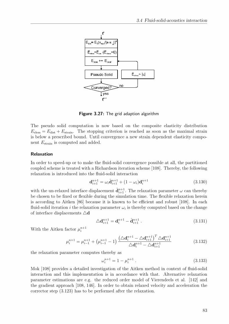
3.4 Fluid-solid-acoustics interaction
Figure 3.27: The grid adaption algorithm
The pseudo solid computation is now based on the composite elasticity distributionEelem = Edist + Estrain. The stopping criterion is reached as soon as the maximal strainis below a prescribed bound. Until convergence a new strain dependent elasticity compo-nent Estrain is computed and added.
Relaxation
In order to speed-up or to make the fluid-solid convergence possible at all, the partitionedcoupled scheme is treated with a Richardson iteration scheme [108]. Thereby, the followingrelaxation is introduced into the fluid-solid interaction
dn+1i+1 = ωid
n+1i+1 + (1− ωi)d
n+1i (3.130)
with the un-relaxed interface displacement dn+1i+1 . The relaxation parameter ω can thereby
be chosen to be fixed or flexible during the simulation time. The flexible relaxation hereinis according to Aitken [86] because it is known to be efficient and robust [108]. In eachfluid-solid iteration i the relaxation parameter ωi is thereby computed based on the changeof interface displacements 4d
4dn+1i+1 = dn+1
i − dn+1i+1 . (3.131)
With the Aitken factor µn+1i
µn+1i = µn+1
i−1 +(µn+1
i−1 − 1) (4dn+1
i −4dn+1i+1
)T 4dn+1i+1
4dn+1i −4dn+1
i+1
(3.132)
the relaxation parameter computes thereby as
ωn+1i = 1− µn+1
i . (3.133)
Mok [108] provides a detailed investigation of the Aitken method in context of fluid-solidinteraction and this implementation is in accordance with that. Alternative relaxationparameter estimations are e.g. the reduced order model of Vierendeels et al. [142] andthe gradient approach [108, 146]. In order to obtain relaxed velocity and acceleration thecorrector step (3.123) has to be performed after the relaxation.
83

3 Numerical fundamentals
Fluid-solid coupled algorithm
The implemented fluid-solid scheme is sketched in Fig. 3.28. To measure the convergence,
Figure 3.28: Flow-chart of the fluid-solid interaction
the relative change of the interface displacements is tested by a stopping criterion. With~d as the solid displacements ~u at the interface
~d = ~u on Γfs (3.134)
the stopping criterion is given by
||di+1 − di||2||di+1||2
< εfsi , (3.135)
whereby εfsi is the defined tolerance.The algorithmic setup of the suggested multifield solver is based on an iterative staggered
scheme as displayed in Fig. 3.28 [108]. To couple the fluid and the solid field the stepsas listed in Algorithm 1 are performed. First of all the predictor step of the mechanicalfield is computed in each time step. The grid mechanics is supplied with these predicteddisplacements and new grid displacements and grid velocities are computed. The fluidfield is solved afterwards on the current grid with the current grid velocity and the currentinterface velocity. Out of the fluid field the fluid loads are computed and applied to themechanical field, which leads to new interface velocities and interface displacements.
Validation example
Altogether six validation examples are discussed to verify the correct implementation ofthe fluid-solid interaction. All fluid simulations are performed with the BDF2 scheme.
84

3.4 Fluid-solid-acoustics interaction
Algorithm 1 Fluid-Solid Schemen = 0, i = 0Read existing restart values for the fluid, the solid and the auxiliary grid field:
fluid: vn and vn−1
solid: un, un and un
grid: rn and rn−1
while n < nmax doPerform the solid predictor step according to (3.121).The predicted solid field variables are taken as initial guess. ⇒ un+1
0 and un+10
while εfsi < εfsi do
Perform grid adaption based on the interface displacements dn+1i
Determine Eelem according to (3.129)while εg
j > εg or j < jmax do
Solve (3.126) ⇒ rn+1i+1
vn+1g i+1 according to (3.128)
Compute maximal element strain εgj
Compute and add strain dependent stiffness Eelem according to (3.4.2)j=j+1
end while ⇒ rn+1i+1 and vn+1
g i+1
Solve the fluid field according to (3.79) on the current domainrn+1
i+1 with the corresponding grid velocity vn+1g i+1
The current interface velocity dn+1i is thereby
inhomogeneous Dirichlet conditions at Γfs. ⇒ vn+1i+1 and pn+1
i+1 .Compute the fluid forces at Γfs according to (3.124) ⇒ fn+1
i+1
Solve the solid field according to (3.122) ⇒ un-relaxed displacements un+1i+1
Compute Aitken relaxation parameter according to (3.133) ⇒ ωi
Relax the solid displacements: un+1i+1 = ωiu
n+1i+1 + (1− ωi)u
n+1i
Perform solid corrector (3.123) ⇒ un+1i+1 and un+1
i+1
εfsi =
||dn+1i+1 −dn+1
i ||2||dn+1
i+1 ||2i = i + 1
end whilen = n + 1
end whileWrite a restart file containing the current fluid, solid and grid information:
fluid: vn and vn−1
solid: un, un and un
grid: rn and rn−1
85

3 Numerical fundamentals
Moving mesh: In order to verify that the applied grid adaption satisfies the geome-try conservation law (2.11) a simple channel flow with a prescribed mesh motion is con-sidered [56]. The geometry of the channel is displayed in Fig. 3.29. The nodes at the
Figure 3.29: Moving channel – grid adaption test case (units in m)
horizontal line (1 m, 1 m)− (2 m, 1 m) inside the domain moves sinusoidally in y-directionry = 0.2 sin(πt) m. In Fig. 3.30a the undeformed and in Fig. 3.30b/c the two extremalmesh deformations are displayed. The frequency is set to f = 0.5 Hz and the time stepsize to 4t = 0.05 s. The maximum mesh velocity in y-direction is thereby higher than themaximum fluid velocity in x-direction:
vx max = 0.5 m/s vgy max = 0.2π ≈ 0.63 m/s . (3.136)
The flow is assumed to be a fully developed channel flow and is therefore analytically
(a) (b) (c)
Figure 3.30: Mesh of the grid adaption test case: (a) undeformed; (b) upper deformationlimit; (c) lower deformation limit.
solvable. A stationary parabolic x-velocity distribution develops. As the y-coordinate ofthe nodes at the moving line changes in time the x-velocity changes as well. The numericalresults and the analytic solution are in compliance, which is shown in Fig. 3.31.
Solid plunger: For the first verification example of the fluid-solid coupling a channelflow [80] is considered as displayed in Fig. 3.32. The fluid domain is discretized with(10 × 1) second order quadrilateral elements. A plunger is positioned on the left side of
86

3.4 Fluid-solid-acoustics interaction
Figure 3.31: Results of the moving channel; x-velocity at (1.5 m/0.5 m)
Figure 3.32: A moving plunger inside a channel to verify the fluid-solid coupling (units in m).
87

3 Numerical fundamentals
that channel. At both horizontal walls slip conditions are applied to obtain a 1d flow, forwhich the momentum conservation reduces to
ρ∂vx
∂t+
∂P
∂x= 0 . (3.137)
The plunger moves during the considered time span (0 s till 2 s) 1 m from left to right witha time step size of 4t = 0.002 s. The x-displacement is prescribed by
ux = 0.5
(t− sin(0.5πt)
0.5π
)m/s . (3.138)
In Fig. 3.33a the prescribed displacement, velocity and acceleration of the plunger is dis-played. The fluid density is set to ρ = 1.0 kg/m3. (3.137) can be solved analytically forthe described plunger movement
P = ρ(10− ux)ux . (3.139)
The action from the solid to the fluid field is verified with this example, as the plunger dis-placement is prescribed, no action of the fluid on the solid field is considered. In Fig. 3.33bthe computed pressure distribution at the fluid-solid interface is compared to the analyticalsolution (3.139). The numerical results thereby coincide with the analytical solutions.
(a) (b)
Figure 3.33: Fluid-solid test case: moving plunger. (a) Prescribed plunger displacement,velocity and acceleration; (b) numerical and analytical pressure at the fluid-solid interface.
Plate: A flexible plate under fluid load [63] as sketched in Fig. 3.34 is the second fluid-solid interaction example. The plate deformation of three different thick plates
dpl = 3, 4, 10mm (3.140)
are compared with each other based on linear elasticity, all with a time step size of4t = 0.01 s. The measure of the deformation is thereby given by the tip displacement
88

3.4 Fluid-solid-acoustics interaction
in stream-wise direction (ux in Fig. 3.34). The mechanical material parameters: elasticitymodulus, Poisson number and density are set to
E = 3.5× 10⁹ Pa , ν = 0 and ρs = 1200 kg/m3 (3.141)
and the fluid mechanical material parameters: dynamic viscosity and density are set to
µ = 0.2 Pa s and ρf = 1 kg/m3 . (3.142)
The fluid domain is meshed with 28160 and the solid with 40 second order quadrilaterals.The fluid-solid interaction simulation is started upon a stationary flow field as displayed in
Figure 3.34: Geometry of 2d plate (units in m)
Fig. 3.35. The tip deflection of the plate is for all three thicknesses displayed in Fig. 3.36.
1
P in hPa
0Figure 3.35: Flow field before fluid-solid interaction - flow around a plate
The results of this simulation are in compliance with those published by Gluck [63].
Lid driven cavity with a flexible bottom: A further fluid-solid interaction verificationexample represents the lid driven cavity with a flexible bottom [108]. Both side walls arethereby fixed and no-slip/no-penetration conditions are applied there except for the upper10 %, where open boundary conditions are applied. At the top boundary an oscillatingx-velocity is enforced
vx = 1.0− cos(0.4πt + π) m/s (3.143)
and the time step size is set to 4t = 0.1 s The geometry is displayed in Fig. 3.37 togetherwith the finite element mesh consisting of 32 × 32 Q2 element. The thin solid bottom
89

3 Numerical fundamentals
Figure 3.36: Plate tip deflection in stream-wise direction for three plate thickness,dpl = 3, 4, 10mm
(a) (b)
Figure 3.37: Lid driven cavity with a flexible bottom (a) Geometric setup (units in m);(b) FEM mesh
90

3.4 Fluid-solid-acoustics interaction
is computed including the geometric non-linearities. The mechanical material parametersare hereby set to
E = 250 Pa , ν = 0 and ρs = 500 kg/m3 (3.144)
and the fluid mechanical material parameters, the dynamic viscosity and density, are setto
µ = 0.01 Pa s and ρf = 1 kg/m3 . (3.145)
The velocity and pressure distribution of the flow in the cavity are displayed on a de-formed fluid mesh in Fig. 3.38a. The movement of the watch-point (0.5/0) is displayed in
5× 10⁻²
P in Pa
−5× 10⁻²(a) (b)
Figure 3.38: Numerical results of the lid driven cavity: (a) streamlines and pressure contourson the deformed fluid domain at t = 27 s (b) y-displacement of the point (0.5 m/0 m).
Fig. 3.38b, both are in compliance with published results [146].
Flag in the downstream of a square cylinder: A further fluid-solid interaction validationexample is given by the flow around a flexible flag in the downstream of a fixed squarecylinder [146]. In the wake of the square a Karman vortex street develops exciting the flagto harmonic oscillations. The time step size is set to 4t = 0.01 s. The geometry of thesetup is displayed in Fig. 3.39. The square cylinder is fixed and the flag in the wake of thecylinder is flexible. The inflow velocity is set to vx = 51.3 m/s. The mechanical materialparameters are set to
E = 2.56× 10⁶ Pa , ν = 0.35 and ρs = 0.1 kg/m3 (3.146)
and the fluid mechanical material parameters, dynamic viscosity and density, are set to
µ = 1.82× 10⁻⁴ Pa s and ρf = 1.18× 10⁻³ kg/m3 . (3.147)
The fluid domain is decomposed into a fixed ΩEuler and a moving part ΩALE around the flagas displayed in Fig. 3.40 together with the fluid and solid mesh. The smooth mesh adaptionof an extremal deformation is shown together with the undeformed fluid mesh in Fig. 3.41.
91

3 Numerical fundamentals
Figure 3.39: Geometrical setup of the flag in the downstream of a square (units in m).
(a) (b)
Figure 3.40: Flag downstream a square: (a) Fluid domain decomposition into a fixed and amoving part. (b) Mesh in the vicinity of the flag.
92

3.4 Fluid-solid-acoustics interaction
(a)
(b)
Figure 3.41: Grid adaption for the flag in the downstream of a square: (a) undeformed; (b)deformed fluid mesh.
93

3 Numerical fundamentals
Figure 3.42: Vertical displacement of the trailing edge of the flag under geometric linear andnon-linear solid mechanics assumption.
The fluid-solid interaction simulation starts with zero fluid velocity. After approximately2 s the flag starts to oscillate with an amplitude of approximately 1 m, see Fig. 3.42. Theflow field is visualized by streamlines on the deformed fluid domain in Fig. 3.43 for thethree marked time steps of Fig. 3.42. Similar to the fluid mechanical example of Sec. 3.1.3eddies appear and detach continously at the square. But now the eddies already appearat the upstream edge. The alternating downstream transported eddies excite the flag toan harmonic oscillation.
A typical convergence progress is shown for this example, for the fluid in Fig. 3.44a andfor the solid field in Fig. 3.44b as well as for the fluid-solid interaction in Fig. 3.44c andthe relaxation parameter ωi in Fig. 3.44d. The fluid field converged on average within 10fluid iterations and the solid within 3 solid iterations. The error measure of the fluid fieldis hereby given by the incremental error
||vi+1 − vi||2 =DOF∑j=1
√(vj
i+1 − vji )
2 (3.148)
with the fluid iteration i. The convergence of the solid field is measured with the strainenergy norm √
4uTk Kk4uk (3.149)
with the solid iteration counter k.
94

3.4 Fluid-solid-acoustics interaction
(a) t1 = 5.66 s
(b) t2 = 5.74 s = t1 + T/4
(c) t3 = 5.81 s = t1 + T/2
Figure 3.43: Fluid-solid interaction results. Streamlines and deformed flag (a)-(c).
95

3 Numerical fundamentals
(a) (b)
(c) (d)
Figure 3.44: Convergence history of the fluid-solid-acoustics benchmark: (a) fluid convergence;(b) solid convergence; (c) fluid-solid convergence; (d) relaxation parameter ωi.
96

3.4 Fluid-solid-acoustics interaction
DFG-Flag: Recently, a DFG-benchmark was established for fluid-solid interactions.Both, measurements [66] and simulations [151] are examined too. Again, a flag is placedin the wake of a cylinder. The cylinder shape is now however circular. At the trailing endof the flag a weight is mounted. The composition of cylinder, sheet and weight is placedin a channel filled with a mixture of Polyglycol and water. The geometry of the setupis displayed in Fig. 3.45. The thickness of the flag is with 40 µm very thin so that the
Figure 3.45: Geometry of the DFG benchmark for fluid-solid interaction (units in mm).
artificially added mass effect, as described in Sec. 2.4.1, is supposed to play a significantrole. The deflection of the flag is measured to be approximately 20 mm in y-direction.The influence of the geometric nonlinearity is supposed to have significant influence onthe deformation. The clamping boundary conditions of the solid field are restricted to theorigin of the cylinder, which is therefore able to rotate. The free rotation degree of freedomis a further complexity for the solid convergence. This fluid-solid interaction benchmarkrepresents therefore a huge challenge for numerical simulation and thus provides an appro-priate problem to verify a new fluid-solid interacting computational scheme. Despite thetraditional way, hints on how to set up the fluid-solid interaction benchmark problem ina simulation are given. It is of advantage to simplify the setup for the onset of this fluid-solid interaction benchmark, e.g. by increasing the solid density, increasing the time stepsize, computing a lower velocity or introducing solid damping to avoid overshooting duringthe start of oscillation. Overshooting often leads to overlapping elements and therefore toan erroneous program stop. All simplifications have to be smoothly switched off after astable oscillation is reached to achieve a higher accuracy. The solid is composed of threematerials: aluminum and two different kind of steels. The mechanical material parametersare
Cylinder : Aluminium E = 1.5× 10¹¹ Pa ν = 0.3 ρs = 4300 kg/m3
Sheet : Steel E = 2.0× 10¹¹ Pa ν = 0.3 ρs = 7855 kg/m3
Weight : Steel E = 2.0× 10¹¹ Pa ν = 0.3 ρs = 7800 kg/m3
and the fluid mechanical material parameters, dynamic viscosity and density, are
Polyglycol− water mixture : µ = 1.64× 10⁻⁴ Pa s ρf = 1050 kg/m3 .
97

3 Numerical fundamentals
The time step size is set to 4t = 5 × 10⁻³ s for the fluid-solid interaction simulation. Assketched in Fig. 3.45 a velocity driven flow is considered with the following inflow profile
vx = 1.45
(1−
(|y|120
)30)
m/s . (3.150)
At the top and the bottom boundary, wall conditions are applied and the outlet is realizedwith open boundary conditions. The stopping criterion of the incremental change of thefluid field is 1× 10⁻³ and the nonlinear solid is assumed to be converged if the error strainenergy is less than 1 × 10⁻⁶. The stopping criterion of the absolute change of interfacedisplacement of the fluid-solid interaction is set to 1 × 10⁻⁵. The fluid-solid interactionsimulation is restarted on a fluid simulation with a small y-velocity of 0.05 m/s at the flagin order to speed up the onset of oscillations. During the fluid-solid coupled run the flagvelocity is according to the fluid-solid interaction condition. The velocity magnitudes andthe deformed fluid domain are shown for one cycle in Fig. 3.46 The Karman vortex streetin the wake of the cylinder governs the flag deformation. The simulated and measuredx-y-displacement of the trailing edge correlates in an acceptable range, see Fig. 3.47a/b. Itcan be seen that the time resolution is quite rough in the simulation Fig. 3.47a. Fluid-solidconvergence problems are observed for smaller time step sizes which are traced back to theartificially added mass effect. The upper and lower bounds of the relaxation parameter isa crucial point for that problem. For the presented simulation, it is forced to be withinthe range 0.01 ≤ ωi ≤ 0.3. The differences between the simulation and the measurementsare supposed to be based on the errors of the time discretization.
Providing now six fluid-solid interaction validation examples, it can be stated that averified fluid-solid interaction scheme is ready to perform phonation simulations. Eventhin solids can be coupled successfully with a fluid flow.
3.4.3 Fluid-acoustics coupling with Lighthill’s acoustic analogy
Mathematically the fluid-acoustics interaction can, e.g., be represented by the Lighthillequation (2.100), see Sec. 2.4.2. In order to describe the finite element discretization ofthe fluid-acoustics coupling, the Lighthill equation is stated once more in index notation
1
c2
∂2Pa
∂t2− ∂2Pa
∂x2i
=∂2Tij
∂xi∂xj
, (3.151)
with appropriate initial and boundary conditions, see [91]. The computational domain Ωis composed of a part on which the fluid mechanics quantities are of relevance Ωf and apure acoustic propagation part Ωa (Ω = Ωf ∪ Ωa). At this stage, it is assumed that theflow variables are known inside the fluid domain Ωf , e.g. due to a previously performedCFD simulation, and therefore the Lighthill tensor is known as well. To develop thevariational form, the Lighthill equation (3.151) is multiplied by a test function q ∈ H1(Ω)and integrated in the whole domain Ω(
1
c2
∂2Pa
∂t2− ∂2Pa
∂x2i
− ∂2Tij
∂xi∂xj
, q
)Ωf∪Ωa
= 0 . (3.152)
98

3.4 Fluid-solid-acoustics interaction
(a) (b) (c)
(d) (e) (f)
(g) (h) (i)
(j) (k) (l)
(m) (n) (o)
Figure 3.46: Velocity magnitude (0− 2.5 m/s) for one cycle (a-o).
99

3 Numerical fundamentals
(a) (b)
Figure 3.47: DFG fluid-solid benchmark; x−y displacement of the trailing edge (71 mm/0 mm)(a) simulation (b) measurement [66].
The integral theorem of Gauss, applied to the spatial derivative of the acoustic pressureyields (
∂2Pa
∂x2i
, q
)Ωf∪Ωa
=
(∂Pa
∂~n, q
)Γfs∪Γa
−(
∂Pa
∂xi
,∂q
∂xi
)Ωf∪Ωa
(3.153)
and applied to the Lighthill tensor, it yields(∂2Tij
∂xi∂xj
, q
)Ωf
=
(∂Tij
∂xj
ni, q
)Γfs
−(
∂Tij
∂xj
,∂q
∂xi
)Ωf
. (3.154)
Based on the continuity equation the term including ∂Tij/∂xj can be substituted by(∂Tij
∂xj
ni, q
)Γfs
= −(
∂Pa
∂~n, q
)Γfs
−(
∂ρvi
∂tni, q
)Γfs
. (3.155)
The last term of (3.155) vanishes with a fixed solid inside the fluid domain and for a flexiblebody the surface integral of the last term has to be resolved and provides the contribution ofthe vibration induced sound. Introducing both partial integrations (3.154) and (3.155) andcombining the surface integrals of the acoustic pressure yields the variational formulationof flow induced noise(
1
c2
∂2Pa
∂t2, q
)Ωf∪Ωa
+
(∂Pa
∂xi
,∂q
∂xi
)Ωf∪Ωa
+
(1
c
∂Pa
∂t, q
)Γa︸ ︷︷ ︸
Absorbing boundary
=
−(
∂Tij
∂xj
,∂q
∂xi
)Ωf︸ ︷︷ ︸
Flow induced sound
−(
ρ∂vi
∂tni, q
)Γfs︸ ︷︷ ︸
Vibrational induced sound
. (3.156)
In (3.156) the relation c (∂Pa/∂~n) = −∂Pa/∂t is utilized [91]. In (3.156) both flow inducedand solid induced sound sources are inherent. It is not necessary to include further terms
100

3.4 Fluid-solid-acoustics interaction
with spatially resolving methods of the source terms as is the case with integral methods.The Galerkin FEM discretization finally yields the following ODE
MPa + DPa + KPa = F , (3.157)
which is discretized in time with the Newmark scheme. As the impact of the acousticquantity on the flow is neglected, a sequential coupling scheme can be applied to resolvefluid-acoustics coupling, see Fig. 3.48.
Figure 3.48: Fluid-acoustics coupled scheme
Validation examples
Kaltenbacher and Escobar [47, 91] provided the validation of flow induced sound simula-tions with CFS++ and external flow solvers. As the developed fluid-solid-acoustics simula-tion scheme is now based on a new flow solver included in CFS++ and the computation ofthe Lighthill sources are thereby introduced as an output result, two validation examplesare discussed in order to verify the correct implementation. These are the co-rotatingvortex pair, which is analytically solvable, and the sound induced by a Karman vortexstreet.
Co-rotating vortex pair
First, the numerical propagation of an acoustic wave by a rotating quadrupole is considered.This is a commonly used test case for the validation of aeroacoustic codes (see e.g. [47, 60,109] and references therein). Within the benchmark, the inhomogeneous wave equation isequipped with acoustic sources, that are obtained from the analytical flow field. The flowfield is induced by the co-rotating vortex pair. This benchmark is reasonable because itprovides a measure for the acoustic field independently from the fluid solver.
The initial configuration of the vortices in the present case is depicted in Fig. 3.49. Theinduced flow field is assumed to be inviscid and incompressible. The two point vorticesare separated by a distance of 2r0 and have a circulation Γv. The vortex cores rotatearound each other with a period of T = 8π2r2
0/Γv. The angular speed of the swirling flowis given by ω = Γv/4πr2
0. The circumferential Mach number is Mar = Γv/4πr0c0. Theflow field of the vortex pair can be determined analytically [47, 109] except at the origin,where a singularity exists. In order to enable a numerical treatment of the problem avortex core model is applied for the flow velocity [47]. The angular velocity of the vortexis set to Γv = 1.00531 m2/s and the radius to r0 = 1 m. The speed of sound is set to
101

3 Numerical fundamentals
Figure 3.49: Schematic drawing of Co-rotating vortices.
c = 1 m/s yielding a rotating Mach number of Mar = 0.08. The considered domain hasan extension of 1000 m × 1000 m in x- and y-direction. The numerical grid is sketchedin Fig. 3.50b. In order to resolve the vortex source accurately, an orthogonal fine gridis clustered around the origin, with 300 × 300 Q2 elements. The adjoining unstructuredmesh is composed of 108000 second order triangular elements which are embedded in astructured mesh of 250000 Q2 elements. The fluid velocities are only prescribed analyticallyin the innermost rectangle (6 m × 6 m) and the Lighthill sources are taken into account
(a) (b) (c)
Figure 3.50: Fluid-acoustics test case: co-rotating vortex pair. Contour plots of the acousticpressure distribution at t = 400 s and mesh: (a) analytical result; (b) FEM mesh; (b) numericalresult
according to (3.156). At the surrounded domain the sound propagation is computed withthe homogeneous wave equation (3.156). A qualitative comparison of the analytical andthe numerical solution is shown by contour plots of the acoustic pressure in Fig. 3.50a/c.Fig. 3.51 shows a quantitative comparison of the pressure distribution along the x-axis ofthe analytical solution with the numerical solution. Overall, the acoustic field is confirmedby the analytical solution. Differences near the origin exist due to the vortex core model.
Sound propagation around a Karman vortex street
The second fluid-acoustics validation example is in principle the same with regard to itssetup as the fluid validation example of Sec. 3.1.3. The flow field is computed with the
102

3.4 Fluid-solid-acoustics interaction
Figure 3.51: Decay of the acoustic pressure values along the x-axis.
developed flow solver as described in Sec. 3.1.3. But now the problem is extended to a fluid-acoustics coupling, for which the acoustic sources and the acoustic pressure distributionare computed. The problem is extended with a surrounding acoustics domain as shownin Fig. 3.52. The resulting acoustic pressure distribution in the near and the far field are
Figure 3.52: Acoustic domain around the cylinder (units in m)
depicted in Fig. 3.53 for a Mach number of Ma = 0.1. The computed dipolar pressurepropagation is in compliance with published results [47, 85].
3.4.4 Solid-acoustics coupling
As explained in the previous section, the sound contribution of an immersed vibratingsolid is captured by (3.156). On solid-acoustics interface where no flow field is adjoiningthe solid-acoustics coupling is captured in the weak form by the boundary integral over
103

3 Numerical fundamentals
Figure 3.53: Acoustic far and near field caused by the Karman vortex street shown in Fig. 3.13and Fig. 3.12 (t = 12 s).
Γfs [91](1
c2
∂2Pa
∂t2, q
)Ωa
+
(∂Pa
∂xi
,∂q
∂xi
)Ωa
+
(1
c
∂Pa
∂t, q
)Γa︸ ︷︷ ︸
Absorbing boundary
= −(
ρ∂2ui
∂t2ni, q
)Γfs︸ ︷︷ ︸
Vibrational induced sound
. (3.158)
(∂2ui/∂t2)ni denotes thereby the mechanical acceleration in normal direction. Herein, theaction of the acoustic pressure on the solid deformation is neglected, so that the solid-acoustics coupling is resolved by a sequential coupling as displayed in Fig. 3.54. The
Figure 3.54: Flow-chart of the solid-acoustics interaction
solid-acoustics coupling is a well verified feature of CFS++, see e.g. [91].
104

3.4 Fluid-solid-acoustics interaction
3.4.5 Fluid-solid-acoustics algorithm
Combining the fluid-solid interaction with the fluid-acoustics coupling finally yields thefluid-solid-acoustics scheme. The iterative coupling scheme to resolve fluid-solid interaction(see Fig. 3.28) can be enhanced with the sequential coupling scheme of the fluid-acousticcoupling ( see Fig. 3.48) as shown in Fig. 3.55 The implementation of the coupling scheme is
Figure 3.55: Fluid-solid-acoustics interaction scheme
depicted in Algorithm 2. The fluid-solid coupling scheme is abbreviated in Algorithm 2 asit is given in detail in Algorithm 1 (see Sec. 3.4.2). The fluid-solid-acoustics coupled schemecomputes the acoustic sound propagation according to Lighthill’s analogy (3.156) after theconverged fluid-solid iteration. To the author’s best knowledge this fully coupled fluid-solid-acoustics interaction scheme is novel. Therefore a first fluid-solid-acoustics coupledbenchmark example is suggested based on the flag in the downstream of a square (see Sec.3.4.2). The flag problem is therefore expanded with an acoustics domain as displayed inFig. 3.56. The geometry of the fluid and the solid domain is as described in Sec. 3.4.2. Theacoustic sound velocity is hereby set to c = 1 m/s. The solid deformation and flow field is asdescribed previously. The velocity magnitude is shown for t = 14.89 s in Fig. 3.57a and thenormalized acoustic pressure is displayed in Fig. 3.57b. In order to investigate the soundgeneration the resolution of the acoustic near field possesses a particular importance. Withtime sequences of the acoustic near field it can be visualized which solid deformation orwhich flow structure is responsible for a certain sound. Fig. 3.57 shows that the near fieldsound correlates with the velocity gradients, therefore the vortex street is the dominantsound generation mechanism of this example. The far field is shown in Fig. 3.58. Thephase relation among the areas with high velocity gradients are important for the far field.
105
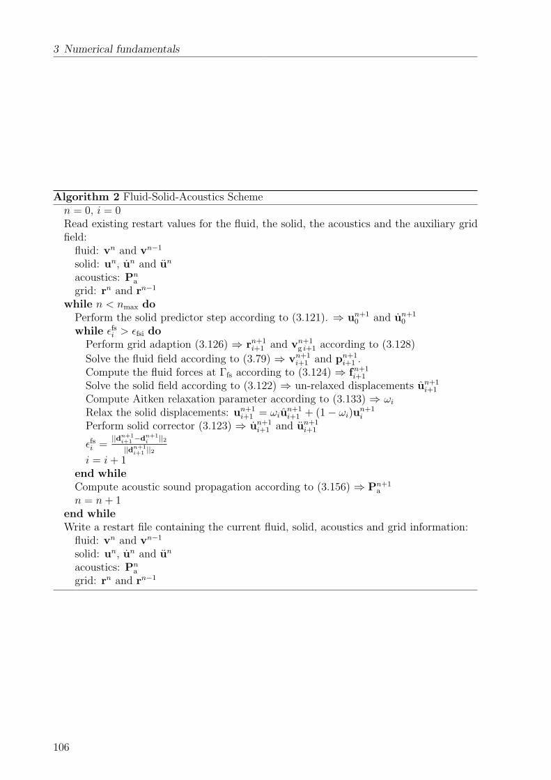
3 Numerical fundamentals
Algorithm 2 Fluid-Solid-Acoustics Schemen = 0, i = 0Read existing restart values for the fluid, the solid, the acoustics and the auxiliary gridfield:
fluid: vn and vn−1
solid: un, un and un
acoustics: Pna
grid: rn and rn−1
while n < nmax doPerform the solid predictor step according to (3.121). ⇒ un+1
0 and un+10
while εfsi > εfsi do
Perform grid adaption (3.126) ⇒ rn+1i+1 and vn+1
g i+1 according to (3.128)
Solve the fluid field according to (3.79) ⇒ vn+1i+1 and pn+1
i+1 .Compute the fluid forces at Γfs according to (3.124) ⇒ fn+1
i+1
Solve the solid field according to (3.122) ⇒ un-relaxed displacements un+1i+1
Compute Aitken relaxation parameter according to (3.133) ⇒ ωi
Relax the solid displacements: un+1i+1 = ωiu
n+1i+1 + (1− ωi)u
n+1i
Perform solid corrector (3.123) ⇒ un+1i+1 and un+1
i+1
εfsi =
||dn+1i+1 −dn+1
i ||2||dn+1
i+1 ||2i = i + 1
end whileCompute acoustic sound propagation according to (3.156) ⇒ Pn+1
a
n = n + 1end whileWrite a restart file containing the current fluid, solid, acoustics and grid information:
fluid: vn and vn−1
solid: un, un and un
acoustics: Pna
grid: rn and rn−1
106

3.4 Fluid-solid-acoustics interaction
Figure 3.56: Fluid, solid and acoustics domain around the flag (units in m)
(a) (b)
Figure 3.57: Results of the fluid-solid-acoustics simulation of the flow around a flag att = 14.89 s: (a) velocity magnitude (0− 90 m/s); (b) normalized acoustic pressure.
Therefore, it is not possible to value the acoustic relevance of a certain sound effect onlyby considering the velocity gradients.
107

3 Numerical fundamentals
Figure 3.58: Acoustic pressure in the far field of the flow around a vibrating flag.
108

4 Fluid-solid-acoustics coupledsimulations of human phonation
4.1 Medical principles
Besides respiration the human respiratory system has a second important functionality:phonation. The possibility to generate sounds is an important factor in social life astherewith information can be exchanged. The larynx plays an important role in thisprocess. The larynx is located inside the throat and connects either the trachea (airway)with the pharynx or the esophagus (food pipe or digestive tract), see Fig. 4.1. The larynxcan be understood as a valve that has two positions, one for breathing, where the tracheais connected to the pharynx and one for swallowing, where the esophagus is connected tothe pharynx. During exhalation the larynx can generate sounds by setting the vocal foldsinto the phonation position. Fig. 4.2 shows the inferior view of the transversal cut throughthe vocal folds schematically in (a) the relaxed , (b) the breathing and (c) the phonationposition from left to right.
Fig. 4.1 shows the basic organs needed for the phonation process with their medicalterminology. The glottis denotes the air gap between the vocal folds and represents animportant anatomical reference for phonation. The following classification is applied todenote regions with respect to the glottis.
sub-glottal below/upstream the glottissupra-glottal above/downstream the glottis
The trachea and the lung are therefore sub-glottal structures, the pharynx and the vocaltract are supra-glottal structures.
The skeleton of the larynx is composed of five cartilages (listed inferior): the epiglottis,the thyroid cartilage, the two arytenoid cartilages and the cricoid cartilage as shown inFig. 4.3a. These cartilages are combined by ligaments as shown in Fig. 4.3b.
The epiglottis has the shape of a leaf and can be moved dorsally to close the larynxentrance. In this configuration, food can pass to the esophagus. After each swallow theepiglottis moves rostrally to the initial position and the larynx entrance is again open forrespiration or phonation.
The thyroid cartilage is composed of two plates which connect ventrally like the bow ofa ship. Those two plates protect the inner larynx elements. A dorsal tilt of the thyroidcartilage relaxes the vocal folds. The thyroid cartilage connected to the cricoid cartilageis inferior, see Fig. 4.3. This connection builds a joint for a tilt motion.
The cricoid cartilage has the shape of a signet ring and builds the supporting element ofthe larynx. The cricoid cartilage is connected with both arytenoid cartilage. The arytenoidcartilage has the shape of a pyramid. The superior connection of the larynx is between thehyoid and the superior thyroid cartilage, see Fig. 4.3b. The cricoid cartilage is connectedinferior as a support of the whole larynx via ligaments to the trachea.
109

4 Human phonation
Figure 4.1: Respiration system of the human body (adapted from [136])
Figure 4.2: Relaxed (a), breathing (b) and phonation (c) position of the vocal folds togetherwith the thyroid and the two arytenoid cartilages.
110

4.1 Medical principles
(a) (b)
Figure 4.3: Skeleton of the larynx (adapted from [125]): (a) the five cartilages; (a) theconnecting ligaments
The two vocal chords, as part of the vocal folds, connect the thyroid cartilage with thetwo arytenoid cartilages, as shown in a transversal cut in Fig. 4.4 and in more detail inFig. 4.5. The tilt motion of the thyroid cartilage and the movements of the two arytenoidcartilages are of major importance in phonation, because they influence the vocal foldstension.
Relative motion of the cartilages is obtained by muscle contraction. The larynx musclesare separated in vocal stiffening muscles and muscles to establish the phonation posi-tion. The location of three vocal fold stiffening muscles are displayed in red color inFig. 4.4 together with their induced arytenoid motion (blue arrow) for a muscle contrac-tion (red arrow). The most important muscle to stiffen the vocal folds is the vocal muscledisplayed in Fig. 4.5.
Fig. 4.6 shows the frontal cut through the larynx. While in Fig. 4.6a the anatomicalcomponents are specified, Fig. 4.6b denotes the sound sources that exist in phonation.Basically three sources exist: the eddy-induced sound which emerges from turbulent flowstructures, the volume-induced sound due to the modulated flow and the sound inducedby vibrating surfaces. The modulated flow provides the main contribution. The air streaminduced by lung compression is guided through the trachea and through the glottis. Theair stream induces the vocal folds to vibrate yielding an oscillating glottis cross sectionalarea. Due to the varying cross sectional area the air stream gets modulated in an acousticrelevant frequency range. This process builds the fundamental frequency of phonation. Inaddition eddy induced and mechanical induced sources exist and it is still an open questionhow these sound sources contributes towards human voice.
111

4 Human phonation
(a) (b) (c)
Figure 4.4: Arytenoid motions caused by stiffening muscles (transversal cut, adapted from[116]) (a) medial motion; (b) lateral rotation; (c) medial rotation
Figure 4.5: Vocal muscle (adapted from [125])
112

4.2 Phonation model
(a) (b)
Figure 4.6: Frontal cut through the larynx (a) anatomical constitution; (a) sound sources
4.2 Phonation model
The geometric assembling of the vocal folds is abutted to the model of Thomson et al. [105,135]. Fig. 4.7 represents an abstraction of the human larynx as sketched in Fig. 4.6. Theview of the larynx is thereby rotated, so that the air streams from the left to the right.The fluid domain is subdivided into two sub-domains: ΩALE and ΩEuler (see Fig. 4.7). In
Figure 4.7: Computational larynx model (distances are given in mm)
the domain ΩALE the fluid-solid interaction takes place, therefore this part of the mesh hasto be adapted within each fluid-solid iteration (ALE mesh). The rest of the fluid domainΩEuler does not need any mesh adaption (Euler mesh). The mechanical field possessesclamping boundary conditions along the line where the vocal folds touch the trachea wall.Fluid-solid interaction conditions are used at the rest of the mechanical boundary. Linearelasticity is assumed for the mechanical field. Absorbing boundary conditions are assumedat the in- and outflow for the acoustics simulation. Inside the whole acoustics domainnodal acoustic loads are applied according to the fluid-acoustics coupling. The time stepsize is set to 4t = 1.0× 10⁻⁴ s.
The 2d finite element mesh consists of second order quadrilateral elements and is shownin Fig. 4.8. The fluid and the acoustic domain are composed of 22872 elements, the
113

4 Human phonation
(a) (b)
Figure 4.8: Mesh around the vocal fold: (a) zoom around the vocal folds; (b) zoom aroundthe glottis
mechanical domain is discretized with 3022 elements and the grid mechanical domainconsist of 14072 elements. The fluid field possess 226074 DOFs, the solid 18380 DOFs,the acoustics 69441 DOFs and the grid adaption 84014 DOFs. The fluid field convergedwithin approximately 5 fluid iterations, and the fluid-solid interaction within 15 iterationsin the mean. The computing time per deformation cycle is approximately 10 hours on fourIntel Xeon 5160 processors of a woodcrest compute-cluster (Overall peak performance:10.4 Tflops/s).
4.3 Vocal fold model
The model of Thomson et al. [135] is improved in order to cover the real physiology moreaccurately. Therefore, the model is divided into three sub-layers [8], the body, the ligamentand the cover as shown in Fig. 4.9. The following abbreviations are used subsequently:vocal fold (vf), sub-glottal (sub), and supra-glottal (supra). The elasticity modulus of
Figure 4.9: Three layer vocal fold model (distances are given in mm)
each layer is selected in such a way that the first vocal fold eigenfrequency is at 100 Hz,see Tab. 4.1. The Poisson number is set to 0.4 for each material.
114

4.4 Fluid mechanical validation of the 2d model with a 3d model
E in kPa
Body 40
Cover 10
Ligament 100
Table 4.1: Vocal fold elasticity modulus
4.4 Fluid mechanical validation of the 2d model with a 3dmodel
The fluid-solid-acoustics coupled simulations of human phonation is in this thesis basedon a 2d plane model. Reasons for this 2d simplification are the high computational effortsof 3d simulations.
In order to evaluate the simplification necessary for the 2d plane case, a comparison with3d flow simulations is performed. Hereby, the finite volume code FASTEST-3D [45, 64] withLES and a 3d larynx model with 8 Mio. control volumes are applied. In the 3d case thewidth of the channel is set to 15 mm. The distribution of the time-averaged stream-wisevelocity vx of the 3d model is displayed together with the 3d streamlines in Fig. 4.10a.The glottis width is thereby set to dGlottis = 1.0 mm. The flow field around the vocal foldis characterized by a jet leaving the glottis. The jet is bent in one direction owing tothe Coanda effect. After a certain distance downstream the glottis, varying in time, thegeneration of vortical structures in the shear layer of the jet can be recognized. This leadsto the transition to turbulence and thus to a broader spectrum of length scales found inthe flow. In the time-averaged flow field the bending of the jet is also visible leading to arecirculation region downstream the vocal folds. As shown in Fig. 4.10a, the recirculationregion possesses an approximately 2d plane distribution. Beside this 2d main stream theflow also possesses minor 3d structures, but the velocity amplitudes in the z-direction areabout ten times smaller than in the x- and y-direction. Near the boundaries z = 0 mmand z = 15 mm the 3d flow structures are thereby more noteworthy than in the midplane.Fig. 4.10b shows that the velocity distribution of the midplane is captured qualitativelywith 2d plane simulations.
The stream-wise velocity and the pressure along the midline are chosen to quantitativelycompare the 2d with the 3d results. Fig. 4.11a/b displays the region near the vocal folds.The velocity profile does not coincide (Fig. 4.11a) as well as the pressure (Fig. 4.11b).Reasons for this difference are the wall effects from the z = 0 mm and the z = 15 mmwall in 3d. These walls, which are present in the 3d setup, produce additional wall shearstresses which the pressure drop has to overcome. The correct pressure distribution has ahigher priority because the ability of the fluid to deform an adjacent solid is of interest.The higher pressure priority is justified because in our case the pressure forces possess a
115
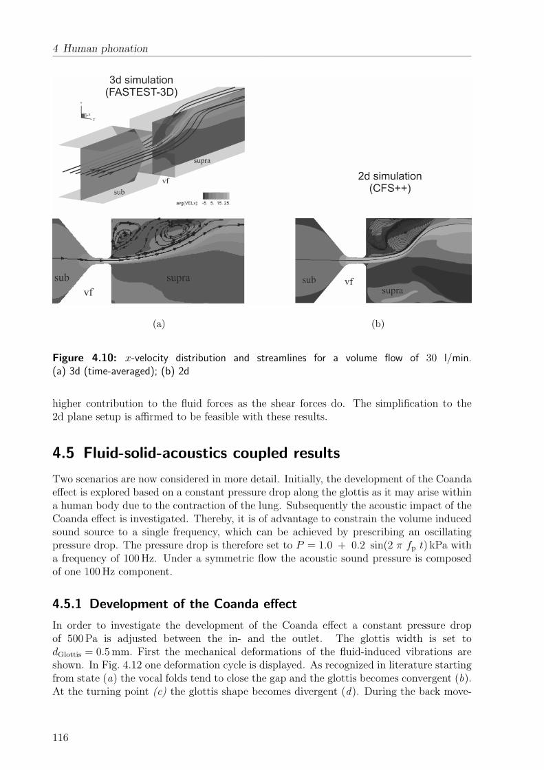
4 Human phonation
(a) (b)
Figure 4.10: x-velocity distribution and streamlines for a volume flow of 30 l/min.(a) 3d (time-averaged); (b) 2d
higher contribution to the fluid forces as the shear forces do. The simplification to the2d plane setup is affirmed to be feasible with these results.
4.5 Fluid-solid-acoustics coupled results
Two scenarios are now considered in more detail. Initially, the development of the Coandaeffect is explored based on a constant pressure drop along the glottis as it may arise withina human body due to the contraction of the lung. Subsequently the acoustic impact of theCoanda effect is investigated. Thereby, it is of advantage to constrain the volume inducedsound source to a single frequency, which can be achieved by prescribing an oscillatingpressure drop. The pressure drop is therefore set to P = 1.0 + 0.2 sin(2 π fp t) kPa witha frequency of 100 Hz. Under a symmetric flow the acoustic sound pressure is composedof one 100 Hz component.
4.5.1 Development of the Coanda effect
In order to investigate the development of the Coanda effect a constant pressure dropof 500 Pa is adjusted between the in- and the outlet. The glottis width is set todGlottis = 0.5 mm. First the mechanical deformations of the fluid-induced vibrations areshown. In Fig. 4.12 one deformation cycle is displayed. As recognized in literature startingfrom state (a) the vocal folds tend to close the gap and the glottis becomes convergent (b).At the turning point (c) the glottis shape becomes divergent (d). During the back move-
116

4.5 Fluid-solid-acoustics coupled results
(a) (b)
Figure 4.11: 2d and 3d simulation results along the midline through the vocal folds (a) stream-wise velocity; (b) pressure
Figure 4.12: Computed deformation cycle of the vocal folds.
117
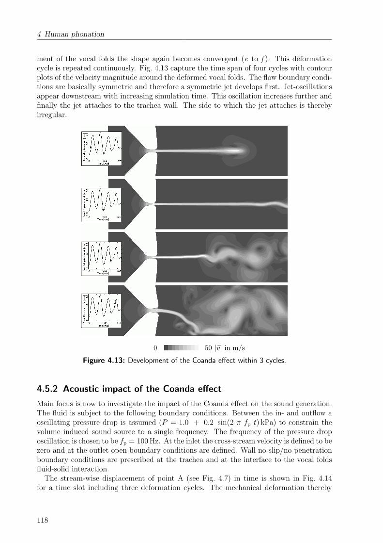
4 Human phonation
ment of the vocal folds the shape again becomes convergent (e to f ). This deformationcycle is repeated continuously. Fig. 4.13 capture the time span of four cycles with contourplots of the velocity magnitude around the deformed vocal folds. The flow boundary condi-tions are basically symmetric and therefore a symmetric jet develops first. Jet-oscillationsappear downstream with increasing simulation time. This oscillation increases further andfinally the jet attaches to the trachea wall. The side to which the jet attaches is therebyirregular.
|~v| in m/s500
Figure 4.13: Development of the Coanda effect within 3 cycles.
4.5.2 Acoustic impact of the Coanda effect
Main focus is now to investigate the impact of the Coanda effect on the sound generation.The fluid is subject to the following boundary conditions. Between the in- and outflow aoscillating pressure drop is assumed (P = 1.0 + 0.2 sin(2 π fp t) kPa) to constrain thevolume induced sound source to a single frequency. The frequency of the pressure droposcillation is chosen to be fp = 100 Hz. At the inlet the cross-stream velocity is defined to bezero and at the outlet open boundary conditions are defined. Wall no-slip/no-penetrationboundary conditions are prescribed at the trachea and at the interface to the vocal foldsfluid-solid interaction.
The stream-wise displacement of point A (see Fig. 4.7) in time is shown in Fig. 4.14for a time slot including three deformation cycles. The mechanical deformation thereby
118

4.5 Fluid-solid-acoustics coupled results
Figure 4.14: Mechanical displacements in stream-wise direction (vertical/x-direction) of pointA (Fig. 4.7) for a time span of 0.03 s
oscillates with 100 Hz. The complete simulation time is set to 0.36 s comprising 36 cyclesand a frequency resolution of 2.8 Hz is obtained, when a Fourier transformation is applied.
A typical velocity magnitude distribution is shown in Fig. 4.15a. The air jet in thedownstream of the glottis is highly unsteady. The wall varies thereby, at which the airjet attaches. The finite element discretization of Lighthill’s acoustic analogy providesnodal acoustic loads [47], representing acoustic point sources. In Fig. 4.15b the spatialdistribution of the nodal acoustic loads due to the velocity field of Fig. 4.15a is displayed.
In order to ensure symmetric flow conditions throughout the whole simulation time, ahemilarynx model is used. The geometry is basically the same as shown in Fig. 4.7. Butthe hemilarynx model considers only one half of the domain. At the midline symmetryconditions are applied. Under symmetric flow conditions a typical velocity distributionand the corresponding nodal acoustic loads are displayed in Fig. 4.15c/d. The main soundgenerating region of the symmetric flow conditions is near the jet front, while with asym-metric conditions the region where the jet attaches the wall has a significant contributionto the sound. Furthermore, the region just downstream the glottis is a noteworthy soundsource (Fig. 4.15b).
The nodal acoustic loads, and therefore also the acoustic field, depend strongly on theair jet dynamics for a developed Coanda effect. This air jet dependency can be exhibitedwith frequency spectra of several field variables. At first, the frequency spectra of theasymmetric case are discussed followed by the symmetric case. In the frequency spectraof the mechanical displacements at point A (Fig. 4.16) and in the fluid velocity at pointB (Fig. 4.17), both in stream-wise direction, the 100 Hz peak is dominant and no othersignificant frequency components are contained. Both the stream-wise displacement andthe stream-wise velocity are mainly dependent on the prescribed pressure oscillation.
The air jet fluctuations introduce additional dependencies. The cross-stream velocity ofpoint D (Fig. 4.7) gives an impression of the air jet fluctuations. In the frequency spectrumof the cross-stream velocity of point D (Fig. 4.18) the 100 Hz does not exist. Therefore,the prescribed pressure oscillation obviously has a minor influence on the cross-streamvelocity at point D. The cross-stream velocity at point D is mainly dependent on the airjet fluctuations, which are highly unsteady (Fig. 4.18). The influence of the jet fluctuationson the acoustic pressure can be seen in Fig. 4.19a. The 100 Hz peak is again dominant,
119

4 Human phonation
(a) (b)
(c) (d)
|~v| in m/s500
Figure 4.15: Velocity and nodal acoustic loads (a) velocity magnitude with Coanda effect; (b)nodal acoustic loads due to (a); (a) velocity magnitude under symmetric flow conditions; (b)nodal acoustic loads due to (c)
Figure 4.16: Mechanical displacements of point A (Fig. 4.7) in stream-wise direction(vertical/x-direction) of the asymmetric case, i. e. with Coanda effect
120
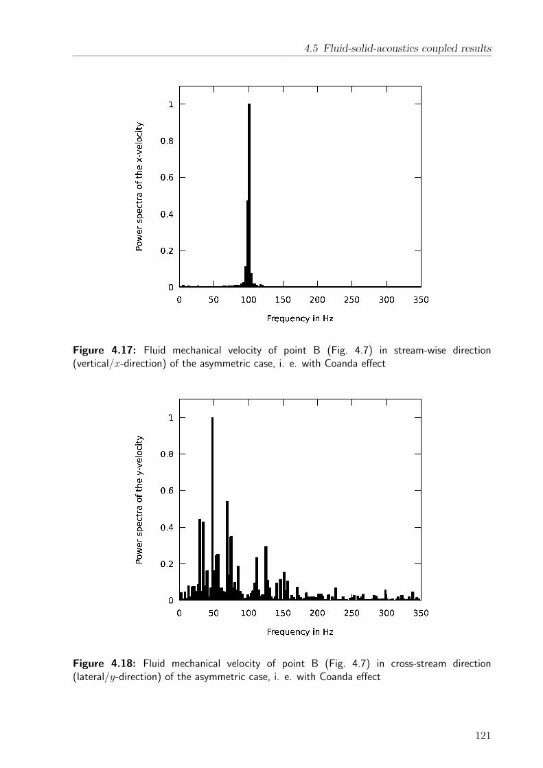
4.5 Fluid-solid-acoustics coupled results
Figure 4.17: Fluid mechanical velocity of point B (Fig. 4.7) in stream-wise direction(vertical/x-direction) of the asymmetric case, i. e. with Coanda effect
Figure 4.18: Fluid mechanical velocity of point B (Fig. 4.7) in cross-stream direction(lateral/y-direction) of the asymmetric case, i. e. with Coanda effect
121

4 Human phonation
(a) (b)
Figure 4.19: Power spectrum of the acoustic pressure of point C (Fig. 4.7) (a) with a developedCoanda effect; (b) under symmetric flow conditions, i. e. without Coanda effect
but strong lower and higher frequency contributions are also recognizable. The spectrumof the acoustic pressure at point C and the spectrum of the cross-stream fluid velocity atpoint D do not correlate, because the cross-stream velocity of point D only gives a roughimpression of the jet fluctuations. However, the acoustic pressure at point C is based onthe complete spatial distributed air jet fluctuations.
Under symmetric flow conditions (hemilarynx model) there is no cross-stream velocity atpoint D and the acoustic pressure spectrum (Fig. 4.19b) contains just the dominant 100 Hzpeak without other significant frequency components, like the stream-wise displacementsat point A and the stream-wise velocity at point B. The frequency spectra of the stream-wise displacement and the stream-wise velocity of the symmetric case are omitted, becausethese quantities have the same frequency spreading as in the asymmetric case (Fig. 4.16and Fig. 4.17).
Broadband acoustic pressure signals (Fig. 4.19) can be produced by a 2d simulation ofharmonically oscillating vocal folds at a frequency of 100 Hz (Fig. 4.16). Remarkable isthereby, that the base signal is strongly enriched especially with lower frequency compo-nents. The Coanda effect is hereby the physical background and a numerical phonationmodel therefore has to be able to capture this effect.
122

5 Summary and outlook
5.1 Summary
The objective of the present dissertation is to develop a computational scheme resolving thefluid-solid-acoustics coupling. As example application the human phonation process is cho-sen. This medical application is a paradigm for a fluid-solid-acoustics coupled phenomenon.At the beginning, the state-of-the-art in simulation of human phonation is reviewed. Manyinvestigations considering either the fluid-solid interaction or the fluid-acoustics interac-tion have been undertaken. So far, no phonation model is based on the completely coupledsystem taking into account the fluid-solid-acoustics interaction. Especially for the inves-tigation of the Coanda effect on phonation, a fully coupled fluid-solid-acoustics model isnecessary.
In order to establish such a computational scheme the physical fundamentals of fluid andsolid mechanics are presented in a uniform framework. The wave propagation in fluids isderived based on fluid mechanical relations and afterwards treated as a separate physicalfield: the acoustic field. The fluid field is mathematically modeled with the incompressibleunsteady Navier-Stokes equations. The solid field is described by the Navier equationstaking geometric nonlinearities into account. The considered acoustic sound propagationis assumed to be linear and, therefore, captured by the standard wave equation. The fluid-solid interaction is resolved in a partitioned fashion in form of a Dirichlet-to-Neumannproblem. Fluid forces thereby act on a solid, which is deformed and influences the velocityof the adhering fluid particles. Due to the solid deformation the fluid domain changesand the fluid mesh needs to be adapted. To perform the grid adaption of the fluid fieldan iterative pseudo solid approach is applied. Therewith, undercut geometries, as e.g.the vocal folds, can be handled. The fluid-acoustics interaction of the scheme is based onLighthill’s acoustic analogy capturing also the sound contribution of an embedded vibratingsolid. Otherwise the solid-acoustics coupling is established by claiming coincident surfaceacceleration.
The developed computational scheme is part of the multifield finite element code CFS++
[93]. The numerical discretization scheme of the fields and their interactions is thereforethe finite element method. At first, the flow solver is implemented and validated. As theGalerkin finite element method involves instabilities for flow problems, a residual-basedstabilized finite element method is applied. The stabilization approach of this schemepossesses an interconnection to turbulence modeling. Altogether, three different time in-tegration schemes are implemented and verified for the fluid field. These are the one-steptheta, the two-step and the 2nd order backward difference method. The two-step methodsolves two linear algebraic systems in each global time step and has therefore approxi-mately the doubled numerical complexity. For comparing the errors of the several schemesa double time step size is chosen for the two-step method. In order to investigate the errorof the respective schemes, the Fourier foot print is given. This gives the dispersion and
123

5 Summary and outlook
dissipation errors inherent in the schemes based on a test problem. The two-step methodwith a time step size of 4ttwo−step = 24t possesses the least dissipative error followed bythe 2nd order backward difference and the backward Euler method. In context of fluid-solid interaction, a double time step size cannot be applied straight away. To gain thecomplete benefit of the two-step method in fluid-solid interaction, the coupling has to betaken into account at the intermediate sub-steps which has not yet been clarified. In thecontext of fluid-solid interaction the time discretization for the fluid field plays a crucialrole. The time step size and the time integration scheme must be chosen carefully becauseof the interconnection with the artificially added mass effect. This effect imposes a lowerbound for the time step size. The analysis of the artificially added mass effect shows thata fluid-solid convergence will be stabilized for a lower accuracy of fluid time discretization.But lower-order fluid time discretization leads to higher numerical errors. So a compromisebetween stability and accuracy has to be found for the problem at hand. The accuracyof the fluid quantities is also important for flow-induced noise because velocity gradientsbuild the acoustic source terms. The 2nd order backward difference scheme has therebya good balance of efficiency, stability and accuracy. The author therefore suggests the2nd order backward difference scheme for applications with fluid-solid interaction and thetwo-step scheme for flow simulations.
The flow simulations of this thesis are linearized with a fixpoint scheme, because itpossesses a more stable convergence rate. The Newton-Raphson scheme indeed has ahigher convergence order, but it is quite sensitive to the initial guess. The performed flowsimulations with the fixpoint scheme converge within three to seven iterations. Thereby,no performance improvement is recognized with the Newton scheme. That is why thefixpoint scheme is utilized.
In order to confirm the correct implementation of the novel flow solver, simulations ofseveral different test setups are performed. Both steady and unsteady flow problems areconsidered. The steady flow through a channel with two different sets of boundary con-ditions are tested: a velocity driven set and a pressure driven set. The pressure dropcondition is of particular importance for phonation simulations as muscle contraction im-poses a pressure drop along the glottis. Thereafter, two different flows around a circularobstacle are discussed. One at Re = 40 resulting in a steady flow and the other at Re = 100for which an unsteady flow develops, known as the Karman vortex street. Finally, simu-lation results of an unsteady flow (Re = 100) around a square are compared to results ofthe finite volume solver FASTEST-3D and a lattice Boltzmann automata. All test examplesprovide excellent compliance. The linear solid mechanics and the linear sound propagationare already included in CFS++. To treat geometric nonlinear solid problems, an updatedLagrangian approach is implemented and validated.
Based on the single field solvers the fluid-solid and the fluid-acoustics coupling are estab-lished within a strongly coupled partitioned scheme. The scheme is validated with severalanalytical and numerical solutions as well as with measurements. Finally the fluid-solid-acoustics coupling scheme is developed. For the first time, it is possible to scrutinize witha high resolution in space, the sound generation of problems driven by fluid-solid interac-tion. The scheme thereby resolves the acoustic near and far field in a spatial manner. Incase of such problems sound can emerge flow or vibrational induced. The novel fluid-solid-acoustics scheme allows accurate numerical simulations of arbitrary complex geometries, toevaluate qualitatively and quantitatively sound sources, in order to reduce e.g. the overallsound radiation of a machinery. A first fluid-solid-acoustics coupled benchmark example
124

5.2 Outlook
based on a flag in the downstream of a square is successfully simulated and explained.
The fluid-solid-acoustics coupled simulations of human phonation is based in this thesison a 2d plane model. Reasons for this 2d simplification are the high computational effortsof 3d simulations. In order to verify the simplification necessary for the 2d plane case, acomparison with 3d flow simulations is performed. The simplification to the 2d plane setupis affirmed to be feasible with these results. The sound sources that exist within phonationare categorized in three different types: the modulated sound, the eddy induced soundand the vibrational induced sound. The modulated source represents a flow induced soundsource like the eddy induced source. It describes the sound emerging from an oscillatingvolume flow, as e.g. in a siren or in human phonation. Such sound sources are very effectivesound emitters. For the first time, these sources are resolved numerically in conjunctionwith the presented computational scheme. The performed phonation simulations capturedthe development of the Coanda effect, i.e. that the air jet tends to touch the tracheawall downstream the glottis after a certain span of time. In the considered setup theCoanda effect develops after three to four oscillation cycles of the vocal folds. Duringthat span of time the glottis does not close completely, so that a case of glottis closureinsufficience exists. Further on, the impact of the Coanda effect on the emerging sound isstudied. The main sound generating region of the symmetric flow conditions is near thejet front, while with asymmetric conditions (with a developed Coanda effect) the regionwhere the jet attaches the wall has a significant contribution to the sound. Furthermore,the region just downstream the glottis is a noteworthy sound source. The nodal acousticloads, and therefore also the acoustic field, depend strongly on the air jet dynamics fora developed Coanda effect. It is detected that the Coanda effect leads to a broadbandsound signal. Remarkable is thereby, that the base signal is strongly enriched especiallywith lower frequency components. The Coanda effect is hereby the physical backgroundand a numerical phonation model therefore has to be able to capture this effect. Based onthese results and on published measurements of hoarse voices the hypothesis arose, thatduring hoarseness the Coanda effect is more severe than in the healthy case. The developedscheme enabled to detect and justify this interconnection between the Coanda effect anddysphonias.
5.2 Outlook
On the basis of this thesis it is now possible to investigate the acoustic impact of thechanges in bio-mechanical material parameters or in geometric conditions induced e.g. bya disease in an spatial accurate manner. Knowing the physical foundations of a disease,the therapies may be optimized. Further on, the substitute voice configuration can beevaluated based on the concluding sound field. However, it is necessary to perform 3dsimulations to treat the substitute voice. This demands a huge increase of computationaleffort. Furthermore, the effect of the trachea stiffness can be included in the phonationmodel.
As the vocal folds normally get in contact with each other, the scheme should be equippedwith the solid mechanical contact. In addition, measurement techniques should be im-proved to determine the mechanical material parameters of the vocal folds in order toverify the applicability of the fractional material model.
In the short term, basic research on simplified geometries can be performed for human
125

5 Summary and outlook
phonation. The long term gain is to simulate the complex geometry that exists in areal body and, in the even longer term, to perform preoperative standardized simulationsin order to plan surgeries - initially based on optimization in an engineering sense andsubsequently in a mathematical sense.
Further technical problems should be considered with the fluid-solid-acoustics schemefor validation reasons and to brighten the knowledge of sound generation in machineries,as e.g. airplanes, trains, trucks and cars. With a better understanding of the generationmechanisms the noise emission may be reduced. The turbo-jet engines, flaps, high buoyantequipment and landing gears could be investigated in the case of an airplane. The wheel-rail contact and flow around the pantograph are application areas of trains and in thecase of road vehicles the wheel-roadway contact and noise induced by the engine could beinvestigated in more detail with the presented fluid-solid-acoustics scheme.
126

Bibliography
[1] ABAQUS, Dassault Systemes Simulia Corp., www.simulia.com.
[2] ADINA, ADINA R&D Inc., www.adina.com.
[3] ANSYS, ANSYS Inc., www.ansys.com.
[4] CFX, ANSYS Inc., www.cfx-germany.com/.
[5] FEAP, A Finite Element Analysis Program, University of California, Berkeley,www.ce.berkeley.edu/∼rlt/feap/.
[6] FLUENT, FLUENT Inc., www.fluent.com.
[7] STAR-CCM+, CD-adapco Group, www.cd-adapco.com/.
[8] F. Alipour, D.A. Berry, and I.R. Titze. A finite-element model of vocal-fold vibration.Journal of the Acoustical Society of America, 108:3003–3012, 2000.
[9] F. Alipour and R.C. Scherer. Flow separation in a computational oscillating vocalfold model. Journal of the Acoustical Society of America, 116:1710–1719, 2004.
[10] J. Altenbach and H. Altenbach. Einfuhrung in die Kontinuumsmechanik (Introduc-tion to continuum mechanics). B. G. Teubner, Stuttgart, 1994.
[11] C. Baiocchi, F. Brezzi, and L.P. Franca. Virtual bubbles and Galerkin-least-squarestype methods. Computer Methods in Applied Mechanics and Engineering, 105:125–141, 1993.
[12] K.-J. Bathe. Finite element procedures. Prentice Hall, 1996.
[13] T. Belytschko, W.K. Liu, and B. Moran. Nonlinear Finite Elements for Continuaand Structures. J. Wiley & Sons Ltd, Chichester, 2000.
[14] D.A. Berry, H. Reininger, F. Alipour, D.M. Bless, and N. Ford. Influence of vocal foldscarring on phonation: Predictions from a finite element model. Annals of Octology,Rhinology and Laryngology, 114:847–852, 2005.
[15] J. Betten. Kontinuumsmechanik (Continuum mechanics). Springer, 2001.
[16] P. Birkholz. 3D-Artikulatorische Sprachsynthese (3d articulatory speech synthesis).PhD thesis, Universitat Rostock, 2005.
[17] P.B. Bochev, M.D. Gunzburger, and R.B. Lehoucq. On stabilized finite elementmethods for the Stokes problem in the small time step limit. Int. J. Numer. Meth.Fluids, 53:573597, 2007.
127

Bibliography
[18] P.B. Bochev, M.D. Gunzburger, and J.N. Shadid. Stability of the SUPG finiteelement method for transient advectiondiffusion problems. Computer Methods inApplied Mechanics and Engineering, 193:23012323, 2004.
[19] D. Braess. Finite Elemente (Finite Elements). Springer, 1991.
[20] S.C. Brenner and L.R. Scott. The mathematical theory of finite element methods.Springer, 2002.
[21] M. Breuer. Direkte Numerische Simulation und Large-Eddy Simulation turbulenterStromungen auf Hochleistungsrechnern (Direct numerical simulation and Large-Eddysimulation of turbulent flows on high performance computers). Habil., UniversityErlangen, 2001.
[22] F. Brezzi, M.O. Bristeau, L.P. Franca, M. Mallet, and G. Roge. A relationshipbetween stabilized finite element methods and the Galerkin method with bubblefunctions. Computer Methods in Applied Mechanics and Engineering, 96:117129,1992.
[23] F. Brezzi and M. Fortin. Mixed and Hybrid Finite Element Methods. Springer, NewYork, 1991.
[24] A.N. Brooks and T.J.R. Hughes. Streamline Upwind/Petrov-Galerkin formula-tions for convection dominated flows with particular emphasis on the incompressibleNavier-Stokes equations. Computer Methods in Applied Mechanics and Engineering,32:199–259, 1982.
[25] P. Causin, J.F. Gerbeau, and F. Nobile. Added-mass effect in the design of parti-tioned algorithms for fluid–structure problems. Computer Methods in Applied Me-chanics and Engineering, 194:4506–4527, 2005.
[26] R.W. Chan and I.R. Titze. Dependence of phonation threshold pressure on vocaltract acoustics and vocal fold tissue mechanics. Journal of the Acoustical Society ofAmerica, 119(4):2351–2362, 2006.
[27] G. Chiandussi, G. Bugeda, and E. Onate. A simple method for automatic updateof finite element meshes. Communications in Numerical Methods in Engineering,16:1–19, 2000.
[28] H.G. Choi, H. Choi, and J.Y. Yoo. A fractional four-step finite element formulation ofthe unsteady incompressible Navier-Stokes equations using SUPG and linear equal-order element methods. Computer Methods in Applied Mechanics and Engineering,143:333–348, 1997.
[29] A.J. Chorin. Numerical solution of the Navier-Stokes equations. Mathematics ofcomputation, 22:745–762, 1968.
[30] A.J. Chorin. On the convergence of discrete approximation to the Navier-Stokesequations. Mathematics of computation, 23:341–353, 1969.
128

Bibliography
[31] R. Codina. A nodal-based implementation of a stabilized finite element method forincompressible flow problems. Int. J. Numer. Meth. Fluids, 33:737–766, 2000.
[32] R. Codina. A stabilized finite element method for generalized stationary incompress-ible flows. Computer Methods in Applied Mechanics and Engineering, 190:2681–2706,2000.
[33] N. Curle. The influence of solid boundaries upon aerodynamic sound. Proceedingsof the Royal Society of London, A231:505–514, 1955.
[34] W. Dahmen, A.J. Kurdila, and P. Oswald. Multiscale wavelet methods for partialdifferential equations. Academic Press Professional, Inc., 1997.
[35] P.A. Davidson. Turbulence - An introduction for scientists and engineers. OxfordUniversity Press, 2005.
[36] M.P. de Vries, H.K. Schutte, A.E.P. Veldman, and G.J. Verkerke. Glottal flowthrough a two-mass model: Comparison of Navier-Stokes solutions with simplifiedmodels. Journal of the Acoustical Society of America, 111(4):1847–1853, 2002.
[37] M.P. de Vries, H.K. Schutte, and G.J. Verkerke. Determination of parameters forlumped parameter models of the vocal fold using a finite element method approach.Journal of the Acoustical Society of America, 106:3620–3628, 1999.
[38] G.Z. Decker and S.L. Thomson. Computational simulations of vocal fold vibration:Bernoulli versus Navier-Stokes. Journal of Voice, 21(3):273–284, 2007.
[39] I. Demirdzic and M. Peric. Space concervation law in finite volume calculations offluid flow. Int. J. Numer. Meth. Fluids, 8:1037–1050, 1988.
[40] W. Dettmer and D. Peric. A computational framework for fluidstructure interac-tion: Finite element formulation and applications. Computer Methods in AppliedMechanics and Engineering, 195:5754–5779, 2006.
[41] J.H. Dirckx, editor. Stedman’s concise medical & allied health dictionary. Williams& Wilkins, 1997.
[42] M. Dollinger, U. Hoppe, F. Hettlich, J. Lohscheller, S. Schuberth, and U. Eysholdt.Vocal fold parameter extraction using the two-mass-model. IEEE J. T. Bio-Med.Eng., 49(8):773–781, 2002.
[43] J. Donea and A. Huerta. Finite element methods for flow problems. Wiley, 2003.
[44] F. Durst. Grundlagen der Stromungsmechanik (Fundamentals in fluid dynamics).Springer, 2006.
[45] F. Durst and M. Schafer. A parallel block-structured multigrid method for theprediction of incompressible flows. Int. J. Numer. Meth. Fluids, 22:549–565, 1996.
[46] B.D. Erath and M.W. Plesniak. The occurence of the Coanda effect in pulsatile flowthrough static models of the human vocal folds. Journal of the Acoustical Society ofAmerica, 120(2):1000–1011, 2006.
129

Bibliography
[47] M. Escobar. Finite-element simulation of flow-induced noise using Lighthill’s acousticanalogy. PhD thesis, University Erlangen-Nuremberg, 2007.
[48] R. Ewert. A Hybrid Computational Aeroacoustics Method to Simulate AirframeNoise. PhD thesis, RWTH Aachen, 2003.
[49] R. Ewert and W. Schroder. Acoustic perturbation equations based on flow decom-position via source filtering. J. Comput. Phys., 188(2):365–398, 2003.
[50] J.H. Ferziger and M. Peric. Computational methods for fluid dynamics. Springer,2002.
[51] J.E. Ffowcs-Williams and D.L. Hawkings. Sound radiation by turbulence and surfacesin arbitrary motions. Philosophical Transactions of the Royal Society of London, 264A:321–342, 1969.
[52] B. Flemisch, M. Kaltenbacher, and B.I. Wohlmuth. Elasto-acoustic and acoustic-acoustic coupling on nonmatching grids. International Journal for Numerical Meth-ods in Engineering, 67(13):1791–1810, 2006.
[53] C.A.J. Fletcher. Computational techniques for fluid dynamics. Springer, 2006.
[54] L. Formaggia, J.F. Gerbeau, F. Nobile, and A. Quateroni. Numerical treatment ofdefective boundary conditions for the Navier-Stokes equations. SIAM Journal onNumerical Analysis, 40(1):376–401, 2002.
[55] Ch. Forster. Robust methods for fluid-structure interaction with stabilised finite ele-ments. PhD thesis, University Stuttgart, 2007.
[56] Ch. Forster, W.A. Wall, and E. Ramm. On the geometric conservation law in tran-sient flow calculations on deforming domains. International Journal for NumericalMethods in Fluids, 50:1369–1379, 2006.
[57] Ch. Forster, W.A. Wall, and E. Ramm. Artificial added mass instabilities in se-quential staggered coupling of nonlinear structures and incompressible viscous flows.Computer Methods in Applied Mechanics and Engineering, 196(7):1278–1293, 2007.
[58] L.P. Franca and C. Farhat. Bubble functions prompt unusual stabilized finite elementmethods. Computer Methods in Applied Mechanics and Engineering, 123:299–308,1995.
[59] L.P. Franca and S.L. Frey. Stabilized finite element methods: II The incompressibleNavier-Stokes equations. Computer Methods in Applied Mechanics and Engineering,99:209–233, 1992.
[60] M. Gebhard. Numerical simulation of fluid-structure-acoustic interactions to analyzehuman voice generation. Master’s thesis, University Erlangen, 2007.
[61] V. Girault and P.-A. Raviart. Finite Element Methods for Navier-Stokes Equations.Springer, 1986.
130
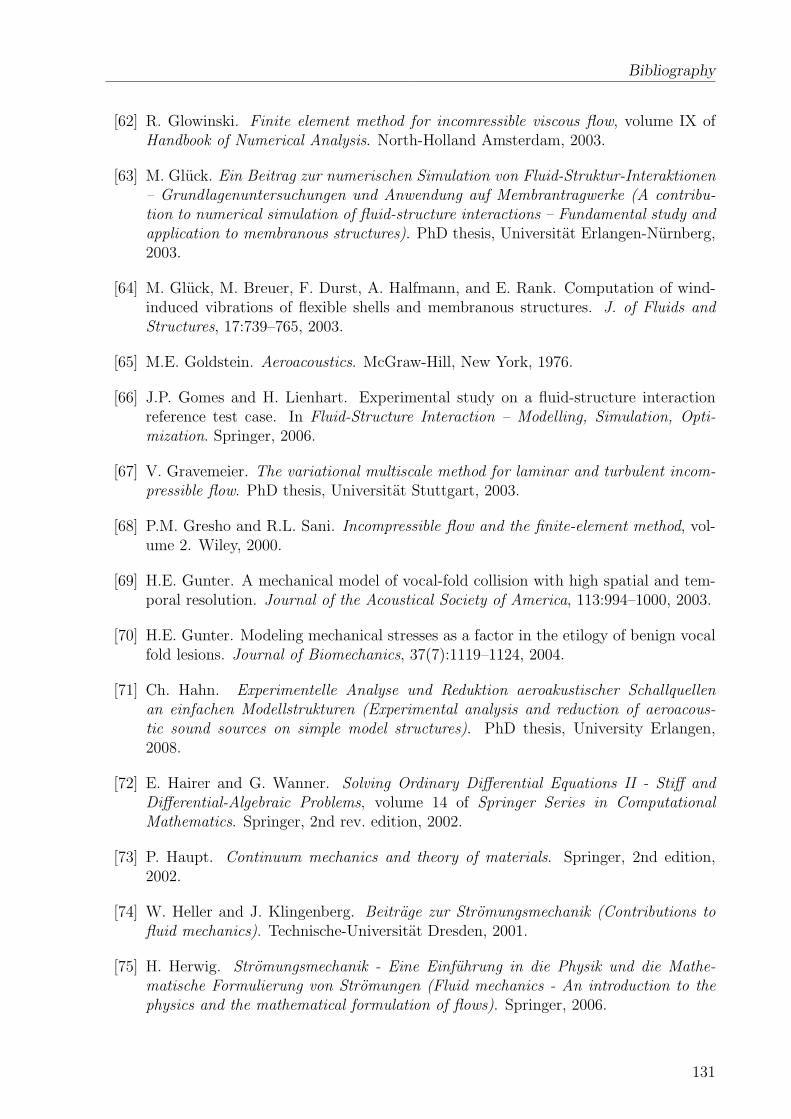
Bibliography
[62] R. Glowinski. Finite element method for incomressible viscous flow, volume IX ofHandbook of Numerical Analysis. North-Holland Amsterdam, 2003.
[63] M. Gluck. Ein Beitrag zur numerischen Simulation von Fluid-Struktur-Interaktionen– Grundlagenuntersuchungen und Anwendung auf Membrantragwerke (A contribu-tion to numerical simulation of fluid-structure interactions – Fundamental study andapplication to membranous structures). PhD thesis, Universitat Erlangen-Nurnberg,2003.
[64] M. Gluck, M. Breuer, F. Durst, A. Halfmann, and E. Rank. Computation of wind-induced vibrations of flexible shells and membranous structures. J. of Fluids andStructures, 17:739–765, 2003.
[65] M.E. Goldstein. Aeroacoustics. McGraw-Hill, New York, 1976.
[66] J.P. Gomes and H. Lienhart. Experimental study on a fluid-structure interactionreference test case. In Fluid-Structure Interaction – Modelling, Simulation, Opti-mization. Springer, 2006.
[67] V. Gravemeier. The variational multiscale method for laminar and turbulent incom-pressible flow. PhD thesis, Universitat Stuttgart, 2003.
[68] P.M. Gresho and R.L. Sani. Incompressible flow and the finite-element method, vol-ume 2. Wiley, 2000.
[69] H.E. Gunter. A mechanical model of vocal-fold collision with high spatial and tem-poral resolution. Journal of the Acoustical Society of America, 113:994–1000, 2003.
[70] H.E. Gunter. Modeling mechanical stresses as a factor in the etilogy of benign vocalfold lesions. Journal of Biomechanics, 37(7):1119–1124, 2004.
[71] Ch. Hahn. Experimentelle Analyse und Reduktion aeroakustischer Schallquellenan einfachen Modellstrukturen (Experimental analysis and reduction of aeroacous-tic sound sources on simple model structures). PhD thesis, University Erlangen,2008.
[72] E. Hairer and G. Wanner. Solving Ordinary Differential Equations II - Stiff andDifferential-Algebraic Problems, volume 14 of Springer Series in ComputationalMathematics. Springer, 2nd rev. edition, 2002.
[73] P. Haupt. Continuum mechanics and theory of materials. Springer, 2nd edition,2002.
[74] W. Heller and J. Klingenberg. Beitrage zur Stromungsmechanik (Contributions tofluid mechanics). Technische-Universitat Dresden, 2001.
[75] H. Herwig. Stromungsmechanik - Eine Einfuhrung in die Physik und die Mathe-matische Formulierung von Stromungen (Fluid mechanics - An introduction to thephysics and the mathematical formulation of flows). Springer, 2006.
131

Bibliography
[76] J.G. Heywood, R. Rannacher, and S. Turek. Artificial boundaries and flux andpressure conditions for the incompressible Navier-Stokes equations. InternationalJournal for Numerical Methods in Fluids, 22:325–352, 1996.
[77] J.O. Hinze. Turbulence. McGraw-Hill, New York, 1975.
[78] G.C.J. Hofmans, G. Groot, M.Ranucci, and G. Graziani. Unsteady flow through in-vitro models of the glottis. Journal of the Acoustical Society of America, 113:1658–1675, 2003.
[79] G.A. Holzapfel. Nonlinear solid mechanics. John Wiley & Sons LTD, Chichester,2000.
[80] B. Hubner. Simultane Analyse von Bauwerk-Wind-Wechselwirkung (Simultaneosanalysis of construction-wind interaction). PhD thesis, Universitat Braunschweig,2003.
[81] T.J.R. Hughes. Multiscale phenomena: Green’s functions, the Dirichlet-to-Neumannformulation, subgrid scale models, bubbles and the origins of stabilized methods.Computer Methods in Applied Mechanics and Engineering, 127:387–401, 1995.
[82] T.J.R. Hughes. The Finite Element Method. Prentice-Hall, New Jersey, 1 edition,2000.
[83] T.J.R. Hughes, G.R. Feijoo, L. Mazzei, and J.-B. Quincy. The variational multiscalemethod - a paradigm for computational mechanics. Computer Methods in AppliedMechanics and Engineering, 166:3–24, 1998.
[84] T.J.R. Hughes, G. Scovazzi, and L.P. Franca. Encyclopedia of Computational Me-chanics: Ch 2 Multiscale and stabilized methods, volume 3. John Wiley & Sons LTD,2004.
[85] O. Inoue and N. Hatakeyama. Sound generation by a two-dimensional circular cylin-der in a uniform flow. J. Fluid Mech, 471:285–314, 2002.
[86] B.M. Irons and R.C. Tuck. A version of the Aitken accelerator for computer iteration.International Journal for Numerical Methods in Engineering, 1:275–277, 1969.
[87] K. Ishizaka and J. Flanagan. Synthesis of voiced sounds from a two-mass model ofthe vocal cords. Bell Syst. Tech. J., 51(6):1233–1268, 1972.
[88] B. Jiang. The least-squares finite element method. Springer, 1998.
[89] V. John. On large-eddy simulation and variational multiscale methods in the nu-merical simulation of turbulent incompressible flows. Applications of Mathematic,51:321–353, 2006.
[90] J. Jovanovic. The statistical dynamics of turbulence. Springer, 2004.
[91] M. Kaltenbacher. Numerical Simulation of Mechatronic Sensors and Actuators.Springer, 2 edition, 2007.
132

Bibliography
[92] M. Kaltenbacher, M. Escobar, S. Becker, and I. Ali. Computational acoustics ofnoise propagation in fluids. Springer, 2008.
[93] M. Kaltenbacher, A. Hauck, S. Triebenbacher, G. Link, and L. Bahr. CFS++: Coupledfield simulation, 2007.
[94] P. Knabner and L. Angermann. Numerik partieller Differentialgleichungen (Numer-ics of partial differential equations). Springer, 2000.
[95] M. Kob. Physical Modeling of the Singing Voice. PhD thesis, RWTH Aachen, 2002.
[96] M.H. Krane. Aeroacoustic production of low-frequency unvoiced speech sounds.Journal of the Acoustical Society of America, 118:410–427, 2005.
[97] M.D. LaMar and J. Xin Y. Qi. Modeling vocal fold motion with a hydrodynamicsemicontinuum model. Journal of the Acoustical Society of America, 114:455–464,2003.
[98] S. Lele. Computational aeroacoustics: A review. AIAA, 1997.
[99] R. Lerch, G. Sessler, and D. Wolf. Technische Akustik - Grundlagen und Anwen-dungen (Technical acoustics - fundamentals and applications). Springer, 2008.
[100] M.J. Lighthill. On sound generated aerodynamically. Part I: General theory. Pro-ceedings of the Royal Society of London, A211:564–587, 1952.
[101] M.J. Lighthill. On sound generated aerodynamically. Part II: Turbulence as a sourceof sound. Proceedings of the Royal Society of London, A222:1–32, 1954.
[102] G. Link. Numerical simulation of fluid-structure interaction. Master’s thesis, Uni-versity Erlangen, 2004.
[103] G. Link, M. Kaltenbacher, and R. Lerch. Numerical simulation to analyze andoptimize the human substitute voice. In C.A. Mota Soares et.al., editor, III EuropeanConference on Computational Mechanics Solids, Structures and Coupled Problems inEngineering, 2006.
[104] G. Link, P. Rademacher, M. Kaltenbacher, and R. Lerch. Viscoelastic modeling ofhuman tissue. In ASIM, 2005.
[105] G. Link, G. Sieber, R. Schwarz, F. Schafer, M. Breuer, S. Becker, andM. Kaltenbacher. Modeling and numerical simulation of human substitute voicegeneration. In G. Greiner, J. Hornegger, H. Niemann, and M. Stamminger, editors,Proceedings of the VMV, 2005.
[106] J.E. Marsden and T.J.R. Hughes. Mathematical foundations of elasticity. Dover,1983.
[107] P. Meyer, R. Wilhelms, and W. Strube. A quasiarticulatory speech synthesizer forgerman language running in real time. Journal of the Acoustical Society of America,86:1070–1082, 1973.
133

Bibliography
[108] D.P. Mok. Partitionierte Losungsansatze in der Strukturdynamik und der Fluid-Struktur-Interaktion (Partitioned analysis schemes in structural dynamics and fluid-structure-interaction). PhD thesis, Universitat Stuttgart, 2001.
[109] E. Muller and F. Obermeie. The spinning vortices as a source of sound. CP-22AGARD, pages 22.1–22.8, 1967.
[110] G. Muller and M. Moser. Taschenbuch der Technischen Akustik (Technical Acous-tics). Springer, 2004.
[111] F. Nobile. Numerical approximation of fluid-structure interaction problems with ap-plication to haemodynamics. PhD thesis, Ecole Politechnique Federale de Lausanne,2001.
[112] E. Onate. Derivation of stabilized equations for numerical solution of advective-diffusive transport and fluid flow problems. Computer Methods in Applied Mechanicsand Engineering, 151(1-2):233–265, 1998.
[113] E. Onate, J. Garcıa, and S.R. Idelsohn. Encyclopedia of Computational Mechanics:Ch 18 Ship hydrodynamics. John Wiley & Sons LTD, 2004.
[114] A.D. Pierce. Acoustics. Acoustical Society of America, 1994.
[115] S.B. Pope. Turbulent flows. Cambridge University Press, 2000.
[116] R. Putz and R. Pabst, editors. Sobotta - Atlas der Anatomie des Menschen (Sobotta- Human anatomy), volume 1. Elsevier Munchen, 22 edition, 2006.
[117] P. Rademacher. Numerical simulation of the biomechanical behaviour of humantissue. Master’s thesis, University Erlangen, 2005.
[118] J. Ramboer, T. Broeckhoven, S. Smirnov, and C. Lacor. Optimization of time inte-gration schemes coupled to spatial discretization for use in CAA applications. Journalof Computational Physics, 213:777–802, 2006.
[119] O. Rasp, J. Lohscheller, M. Dollinger, U. Eysholdt, and U. Hoppe. The pitch raiseparadigm: A new task for real-time endoscopy of non-stationary phonation. FoliaPhoniatr Logo, 58(3):175–185, 2006.
[120] M.O. Rosa, J.C. Pereira, M. Grellet, and A. Alwan. A contribution to simulatinga three-dimensional larynx model using the finite element method. Journal of theAcoustical Society of America, 114(5):2893–2905, 2003.
[121] T.D. Rossing. Handbook of acoustics. Springer, 2007.
[122] J.C. Rotta. Turbulente Stromungen (Turbulent flows). Teubner, 1972.
[123] A. Russo. Streamline-upwind Petrov/Galerkin method (SUPG) vs residual-free bub-bles (RFB). Computer Methods in Applied Mechanics and Engineering, 195:1608–1620, 2006.
134

Bibliography
[124] R.L. Sani and P.M. Gresho. Resume and remarks on the open boundary conditionminisymposium. Int. J. Numer. Meth. Fluids, 18:983–10008, 1994.
[125] A. Sarikas. Funktionelle Anatomie des Menschen (Functional anatomy of the hu-man). Mencke-Blaesing, Erlangen, 7 edition, 2003.
[126] F. Schafer, S. Kniesburges, T. Uffinger, S. Becker, J. Grabinger, G. Link, andM. Kaltenbacher. Numerical simulation of fluid-structure- and fluid-structure-acoustic interaction based on a partitioned coupling scheme. In High PerformanceComputing in Science and Engineering Munich 2007, Transactions of the Third JointHLRB and KONWIHR Result and Reviewing Workshop, Leibniz-RechenzentrumMnchen (LRZ), Garching. Springer, 2007.
[127] O. Schenk and K. Gartner. Solving unsymmetric sparse systems of linear equationswith PARDISO. J. of Future Generation Computer Systems, 20(3):475–487, 2004.
[128] H. Schlichting and K. Gersten. Grenzschicht-Theorie (Boundary layer theory).Springer, 2006.
[129] A. Schmidt. Finite-Elemente-Formulierungen viskoelastischer Werkstoffe mit frak-tionalen Zeitableitungen (Finite element formulation of viscoelastic materials withfractional time derivatives). PhD thesis, University Stuttgart, 2003.
[130] D. Shinwari, R.C. Scherer, K.J. De Witt, and A.A. Afjeh. Flow visualization andpressure distribution in a model of the glottis with a symmetric and oblique divergentanle of 10 degrees. Journal of the Acoustical Society of America, 113(1):487–497,2003.
[131] C. Tao, J.J. Jiang, and Y. Zhang. Simulation of vocal fold impact pressures with aself-oscillating finite-element model. Journal of the Acoustical Society of America,119(6):3987–3994, 2003.
[132] L. Terentiev. The turbulence closure model based on linear anisotropy invariantanalysis. PhD thesis, University Erlangen, 2006.
[133] T.E. Tezduar, S. Mittal, S.E. Ray, and R. Shih. Incompressible flow computa-tions with stabilized bilinear and linear equal-order-interpolation velocity-pressureelements. Computer Methods in Applied Mechanics and Engineering, 95:221–242,1992.
[134] T.E. Tezduyar. Encyclopedia of Computational Mechanics: Ch 17 Finite elementmethods for fluid dynamic with moving boundaries and interfaces. John Wiley &Sons LTD, 2004.
[135] S.L. Thomson, L. Mongeau, and S.H. Frankel. Physical and numerical flow-excitedvocal fold models. In 3rd International Workshop MAVEBA, pages 147–150. FirenzeUniversity Press, 2003. ISBN 88-8453-154-3.
[136] I.R. Titze. Principles of voice production. Prentice Hall, 1994.
135

Bibliography
[137] I.R. Titze. The myoelastic aerodynamic theora of phonation. The National Centerof Voice and Speech, Denver, 2006.
[138] I.R. Titze and H.S. Story. Rules for controlling low-dimensional vocal fold modelswith muscle activation. Journal of the Acoustical Society of America, 112(3):1064–1076, 2002.
[139] S. Turek. A comparative study of time-stepping techniques for the incompressibleNavier-Stokes equations : From fully implicit non-linear schemes to semi-implicitprojection methods. Int. J. Numer. Meth. Fluids, 22:987–1011, 1996.
[140] S. Turek. Efficient Solvers for Incompressible Flow Problems: An Algorithmic andComputational Approach. Springer, 1999.
[141] S. Turek, L. Rivkind, J. Hron, and R. Glowinski. Numerical analysis of a new time–stepping theta–scheme for incompressible flow simulations. Technical Report 282,FB Mathematik, Universitat Dortmund, 2005.
[142] J. Vierendeels, K. Dumontb, and P.R. Verdonckb. A partitioned strongly coupledfluid-structure interaction method to model heart valve dynamics. Journal of Com-putational and Applied Mathematics, 218:602–609, 2008.
[143] P. Sidlof. Fluid-structure interaction in human vocal folds. PhD thesis, CharlesUniversity Prag, 2007.
[144] C. Wagner, T. Huttl, and P. Sagaut. Large-Eddy Simulation for Acoustics. Cam-bridge University Press, New York, 2007.
[145] E. Walhorn. Ein simultanes Berechnungsverfahren fur Fluid-Struktur-Wechselwirkungen mit finiten Raum-Zeit-Elementen (A simultanous computationapproache with finite space-time elements for fluid-solid interaction). PhD thesis,University Braunschweig, 2002.
[146] W.A. Wall. Fluid-Struktur-Interaktion mit stabilisierten Finiten Elementen (Fluid-structure interaction with stabilized finite-elements). PhD thesis, UniversitatStuttgart, 1999.
[147] J.E. Ffowcs Williams and D.L. Hawkings. Sound generation by turbulence andsurfaces in arbitrary motion. Philosophical Transactions of the Royal Society ofLondon, Series A, Mathematical and Physical Sciences, 264 (1151):321–342, 1969.
[148] K. Willner. Kontinuums- und Kontaktmechanik (Continuums and contact mechan-ics). Springer, 2003.
[149] P. Wriggers. Nichtlineare Finite-Elemente-Methoden (Non-linear finite elementmethods). Springer, 2001.
[150] T. Wurzbacher, R. Schwarz, M. Dollinger, U. Hoppe, U. Eysholdt, and J. Lohscheller.Model based classification of non-stationary vocal fold vibrations. Journal of theAcoustical Society of America, 120(2):1012–1027, 2006.
136

Bibliography
[151] S. Yigit, M. Schafer, and M. Heck. Grid movement techniques and their influence onlaminar fluid structure interaction computations. Journal of Fluids and Structures,24(6):14, 2008.
[152] C. Zhang, W. Zhao, S. H. Frankel, and L. Mongeau. Computational aeroacousticsof phonation, Part II: Effects of flow parameter and ventricular folds. Journal of theAcoustical Society of America, 112:2147–2154, 2002.
[153] Z. Zhang, L. Mongeau, S.H. Franke, and S.L. Thomson. Sound generation by steadyflow through glottis-shaped orfices. Journal of the Acoustical Society of America,116(3):1720–1728, 2004.
[154] W. Zhao, S.H. Frankel, and L. Mongeau. Numerical simulation of sound from con-fined pulsating axisymmetric jets. AIAA Journal, 39(10):1868–1874, 2001.
[155] W. Zhao, C. Zhang, S.H. Frankel, and L. Mongeau. Computational aeroacousticsof phonation, Part I: Computational methods and sound generation mechanisms.Journal of the Acoustical Society of America, 112:2134–2146, 2002.
[156] 0.C. Zienkiewicz and R.L. Taylor. The finite element method: Volume I, The basis.Butterworth Heinemann, 2000.
[157] 0.C. Zienkiewicz and R.L. Taylor. The finite element method: Volume II, Solidmechanics. Butterworth Heinemann, 2000.
[158] 0.C. Zienkiewicz and R.L. Taylor. The finite element method: Volume III, Fluiddynamics. Butterworth Heinemann, 2000.
137

List of Figures
1.1 Modeling of fluid-solid-acoustics interaction . . . . . . . . . . . . . . . . . 2
2.1 Continuum mechanical relations to derive a closed mathematical model. . . 9
2.2 A body B composed of particles < . . . . . . . . . . . . . . . . . . . . . . . 11
2.3 Domain and boundary definition . . . . . . . . . . . . . . . . . . . . . . . . 11
2.4 Reference systems . . . . . . . . . . . . . . . . . . . . . . . . . . . . . . . . 13
2.5 Path- and streamline to visualize a flow field. . . . . . . . . . . . . . . . . . 16
2.6 Outer forces ~f yield inner stresses ~t . . . . . . . . . . . . . . . . . . . . . . 17
2.7 Anisotropy invariant map of second and third invariant . . . . . . . . . . . 28
2.8 Rheological bodies: Hooke, Newton and fractional body . . . . . . . . . . . 32
2.9 Geometry of a fluid-solid interacting model problem [25] . . . . . . . . . . 36
2.10 Methods in computational aeroacoustics (according to [144]) . . . . . . . . 37
3.1 Analytical and numerical solution of (3.8) . . . . . . . . . . . . . . . . . . 44
3.2 Test function wi. (a) standard Galerkin FEM; (b) with upwinding. . . . . 46
3.3 Dissipation error of the BE, the two-step and the BDF2 method . . . . . . 60
3.4 Flow-through channel (a) computational domain of the channel (units inm); (b) finite element mesh. . . . . . . . . . . . . . . . . . . . . . . . . . . 62
3.5 Numerical results of the channel flow (a) pressure P (b) velocity vx. . . . . 62
3.6 Numerical and analytic results of the channel flow (a) pressure in x-directionalong y = 0.5 m (b) velocity vx in y-direction along x = 1 m. . . . . . . . . 63
3.7 A Karman vortex street around the island Guadalupe (picture from NASAwww.nasa.com). . . . . . . . . . . . . . . . . . . . . . . . . . . . . . . . . . 64
3.8 Flow around a cylinder. (a) Geometry of the fluid domain (units in m) (b)FEM mesh. . . . . . . . . . . . . . . . . . . . . . . . . . . . . . . . . . . . 64
3.9 Streamlines on pressure for Re = 40 and the specification of the detachingangle αr and the recirculation length Lr. . . . . . . . . . . . . . . . . . . . 65
3.10 Pressure along the cylinder wall for Re = 40. . . . . . . . . . . . . . . . . . 66
3.11 Normalized velocity and pressure at the point (2.7×10⁻³ m/0 m) for Re = 100. 66
3.12 Streamlines of a Karman vortex street in the wake of a cylinder at Re = 100 68
3.13 Numerical results at t1 for Re = 100 (a) pressure (b) velocity magnitude. . 69
3.14 Normalized velocity and pressure for Re = 100 (a) along the horizontalcenterline (y = 0 m); (b) along the vertical line (x = 0.001 m) for the timestep t2 = 64.768 s . . . . . . . . . . . . . . . . . . . . . . . . . . . . . . . . 69
3.15 Flow around a square (a) geometry of the fluid domain (units in m); (b)FEM mesh around the square. . . . . . . . . . . . . . . . . . . . . . . . . . 70
3.16 Streamlines of a Karman vortex street in the wake of a square at Re = 100showing one half cycle of the eddy detaching in three time steps. . . . . . . 71
138

List of Figures
3.17 Velocity along two vertical lines in the flow field, through the center of thesquare (x = 0 m) and inside the wake (x = 4 m): (a) stream-wise velocityvx; (b) cross-stream velocity vy. . . . . . . . . . . . . . . . . . . . . . . . . 72
3.18 Velocity along the horizontal centerline (y = 0 m): (a) stream-wise velocityvx; (b) cross-stream velocity vy. . . . . . . . . . . . . . . . . . . . . . . . . 72
3.19 Non-linear benchmark example: the cantilever beam (a) geometry and load(units in m); (b) deformed and undeformed FEM mesh. . . . . . . . . . . . 75
3.20 Monolithic and partitioned coupling scheme . . . . . . . . . . . . . . . . . 773.21 Field coupling types: (a) surface coupling; (b) volume coupling. . . . . . . 783.22 The fluid-solid interface elements . . . . . . . . . . . . . . . . . . . . . . . 783.23 Deformed and undeformed solid flag . . . . . . . . . . . . . . . . . . . . . . 793.24 Grid adaption . . . . . . . . . . . . . . . . . . . . . . . . . . . . . . . . . . 803.25 ALE- and Euler domain of fluid . . . . . . . . . . . . . . . . . . . . . . . . 813.26 Grid adaption in the vicinity of the vocal folds . . . . . . . . . . . . . . . . 823.27 The grid adaption algorithm . . . . . . . . . . . . . . . . . . . . . . . . . . 833.28 Flow-chart of the fluid-solid interaction . . . . . . . . . . . . . . . . . . . . 843.29 Moving channel – grid adaption test case (units in m) . . . . . . . . . . . . 863.30 Mesh of the grid adaption test case: (a) undeformed; (b) upper deformation
limit; (c) lower deformation limit. . . . . . . . . . . . . . . . . . . . . . . . 863.31 Results of the moving channel; x-velocity at (1.5 m/0.5 m) . . . . . . . . . 873.32 A moving plunger inside a channel to verify the fluid-solid coupling (units
in m). . . . . . . . . . . . . . . . . . . . . . . . . . . . . . . . . . . . . . . 873.33 Fluid-solid test case: moving plunger . . . . . . . . . . . . . . . . . . . . . 883.34 Geometry of 2d plate (units in m) . . . . . . . . . . . . . . . . . . . . . . . 893.35 Flow field before fluid-solid interaction - flow around a plate . . . . . . . . 893.36 Plate tip deflection in stream-wise direction for three plate thickness,
dpl = 3, 4, 10mm . . . . . . . . . . . . . . . . . . . . . . . . . . . . . . . 903.37 Lid driven cavity with a flexible bottom . . . . . . . . . . . . . . . . . . . 903.38 Numerical results of the lid driven cavity . . . . . . . . . . . . . . . . . . . 913.39 Geometrical setup of the flag in the downstream of a square (units in m). . 923.40 Flag downstream a square: Fluid domain decomposition into a fixed and a
moving part and mesh in the vicinity of the flag. . . . . . . . . . . . . . . . 923.41 Grid adaption for the flag in the downstream of a square . . . . . . . . . . 933.42 Vertical displacement of the trailing edge of the flag under geometric linear
and non-linear solid mechanics assumption. . . . . . . . . . . . . . . . . . . 943.43 Fluid-solid interaction results. Streamlines and deformed flag . . . . . . . . 953.44 Convergence history of the fluid-solid-acoustics benchmark. . . . . . . . . . 963.45 Geometry of the DFG benchmark for fluid-solid interaction (units in mm). 973.46 Velocity magnitude (0− 2.5 m/s) for one cycle (a-o). . . . . . . . . . . . . 993.47 DFG fluid-solid benchmark; measured and simulated x− y displacement of
the trailing edge . . . . . . . . . . . . . . . . . . . . . . . . . . . . . . . . . 1003.48 Fluid-acoustics coupled scheme . . . . . . . . . . . . . . . . . . . . . . . . 1013.49 Schematic drawing of Co-rotating vortices. . . . . . . . . . . . . . . . . . . 1023.50 Fluid-acoustics test case: co-rotating vortex pair . . . . . . . . . . . . . . . 1023.51 Decay of the acoustic pressure values along the x-axis. . . . . . . . . . . . . 1033.52 Acoustic domain around the cylinder (units in m) . . . . . . . . . . . . . . 103
139
List of Figures
3.53 Acoustic far and near field caused by the Karman vortex street shown inFig. 3.13 and Fig. 3.12 (t = 12 s). . . . . . . . . . . . . . . . . . . . . . . . 104
3.54 Flow-chart of the solid-acoustics interaction . . . . . . . . . . . . . . . . . 1043.55 Fluid-solid-acoustics interaction scheme . . . . . . . . . . . . . . . . . . . . 1053.56 Fluid, solid and acoustics domain around the flag (units in m) . . . . . . . 1073.57 Results of the fluid-solid-acoustics simulation of the flow around a flag . . . 1073.58 Acoustic pressure in the far field of the flow around a vibrating flag. . . . . 108
4.1 Respiration system of the human body (adapted from [136]) . . . . . . . . 1104.2 Relaxed (a), breathing (b) and phonation (c) position of the vocal folds
together with the thyroid and the two arytenoid cartilages. . . . . . . . . . 1104.3 Skeleton of the larynx . . . . . . . . . . . . . . . . . . . . . . . . . . . . . 1114.4 Arytenoid motions caused by stiffening muscles . . . . . . . . . . . . . . . 1124.5 Vocal muscle (adapted from [125]) . . . . . . . . . . . . . . . . . . . . . . . 1124.6 Frontal cut through the larynx . . . . . . . . . . . . . . . . . . . . . . . . . 1134.7 Computational larynx model (distances are given in mm) . . . . . . . . . . 1134.8 Mesh around the vocal fold . . . . . . . . . . . . . . . . . . . . . . . . . . 1144.9 Three layer vocal fold model (distances are given in mm) . . . . . . . . . . 1144.10 x-velocity distribution and streamlines for a volume flow of 30 l/min.
(a) 3d (time-averaged); (b) 2d . . . . . . . . . . . . . . . . . . . . . . . . . 1164.11 2d and 3d simulation results along the midline through the vocal folds . . . 1174.12 Computed deformation cycle of the vocal folds. . . . . . . . . . . . . . . . 1174.13 Development of the Coanda effect within 3 cycles. . . . . . . . . . . . . . . 1184.14 Mechanical displacements in stream-wise direction (vertical/x-direction) of
point A (Fig. 4.7) for a time span of 0.03 s . . . . . . . . . . . . . . . . . . 1194.15 Velocity and nodal acoustic loads for a developed Coanda effect and under
symmetric conditions . . . . . . . . . . . . . . . . . . . . . . . . . . . . . . 1204.16 Mechanical displacements of point A (Fig. 4.7) in stream-wise direction
(vertical/x-direction) of the asymmetric case, i. e. with Coanda effect . . . 1204.17 Fluid mechanical velocity of point B (Fig. 4.7) in stream-wise direction
(vertical/x-direction) of the asymmetric case, i. e. with Coanda effect . . . 1214.18 Fluid mechanical velocity of point B (Fig. 4.7) in cross-stream direction
(lateral/y-direction) of the asymmetric case, i. e. with Coanda effect . . . 1214.19 Power spectrum of the acoustic pressure of point C (Fig. 4.7) . . . . . . . . 122
140

List of Tables
1.1 Progress of numerical phonation models. . . . . . . . . . . . . . . . . . . . 3
2.1 Characterization of flows by the Mach number Ma . . . . . . . . . . . . . 202.2 Characteristic numbers of fluid mechanics . . . . . . . . . . . . . . . . . . 26
3.1 Momentum stabilization operators LstabM for different schemes. . . . . . . . 52
3.2 y-displacement of the tip of the beam in (m). . . . . . . . . . . . . . . . . 76
4.1 Vocal fold elasticity modulus . . . . . . . . . . . . . . . . . . . . . . . . . . 115
141


Ein Finite-Elemente-Verfahren fur
Fluid-Struktur-Akustik-Interaktionen
und dessen Anwendung auf die
menschliche Phonation
Der Technischen Fakultat der
Universitat Erlangen-Nurnberg
zur Erlangung des Grades
DOKTOR - INGENIEUR
vorgelegt von
Gerhard Link
Erlangen, 2008

Curriculum Vitae
Personal Data
Name: Gerhard Link
Date of birth: November 7, 1974
Place of birth: Weißenburg i. Bay., Germany
Education
1993 Diploma from secondary school,Technical college Weißenburg i. Bay
(10/1993 — 09/1994 Military Service, Goslar and Neuburg a. D.)
10/1994 — 04/1999 Dipl.-Ing. (FH) in Mechanical Engineering,Georg Simon Ohm Universityof Applied Science Nuremberg
04/2002 — 06/2004 M.Sc. in Computational Engineering(graduation with distinction),Friedrich Alexander University Erlangen-Nuremberg
Professional Experience
04/1999 — 06/2004 Computational Engineer,MAN AG, Nuremberg(part time from 04/2002)
since 07/2004 Research fellow,Department of Sensor Technology,University Erlangen-Nuremberg