contentsgesbert/papers/mimo_lte.pdf · umts long term evolution: from ... ‡huawei technologies,...
TRANSCRIPT

1

2
Contents
1 Multiple antenna techniques 1
2 Multiple antenna techniques 32.1 Fundamentals of Multiple antenna Theory . . . . . . . . . . . . . . . . . . . 3
2.1.1 Overview . . . . . . . . . . . . . . . . . . . . . . . . . . . . . . . . 32.1.2 MIMO signal model . . . . . . . . . . . . . . . . . . . . . . . . . . 62.1.3 Single-user MIMO techniques . . . . . . . . . . . . . . . . . . . . . 7
2.1.3.1 Optimal transmission over MIMO systems . . . . . . . . . 72.1.3.2 Beamforming with single antenna transmitter or receiver . 82.1.3.3 Spatial multiplexing without channel knowledge at the trans-
mitter . . . . . . . . . . . . . . . . . . . . . . . . . . . . . 102.1.3.4 Diversity . . . . . . . . . . . . . . . . . . . . . . . . . . . 11
2.1.4 Multi-user techniques . . . . . . . . . . . . . . . . . . . . . . . . . . 122.1.4.1 Comparing single-user and multi-user MIMO . . . . . . . 122.1.4.2 Techniques for single-antenna UEs . . . . . . . . . . . . . 132.1.4.3 Techniques for multiple-antenna UEs . . . . . . . . . . . . 142.1.4.4 Comparing single-user and multi-user capacity . . . . . . . 14
2.2 MIMO schemes in LTE . . . . . . . . . . . . . . . . . . . . . . . . . . . . . 162.2.1 Practical considerations . . . . . . . . . . . . . . . . . . . . . . . . 162.2.2 Single-user schemes . . . . . . . . . . . . . . . . . . . . . . . . . . 19
2.2.2.1 Transmit diversity schemes . . . . . . . . . . . . . . . . . 192.2.2.2 Beamforming schemes . . . . . . . . . . . . . . . . . . . 212.2.2.3 Spatial multiplexing schemes . . . . . . . . . . . . . . . . 222.2.2.4 Feedback computation and signalling . . . . . . . . . . . . 27
2.2.3 Multi-user schemes . . . . . . . . . . . . . . . . . . . . . . . . . . . 282.2.3.1 Precoding strategies and supporting signalling . . . . . . . 292.2.3.2 Calculation of Precoding Vector Indicator (PVI) and CQI . 312.2.3.3 User selection mechanism . . . . . . . . . . . . . . . . . . 352.2.3.4 Receiver spatial equalizers . . . . . . . . . . . . . . . . . 36
2.2.4 Physical-layer MIMO performance . . . . . . . . . . . . . . . . . . 372.2.4.1 Precoding Performance . . . . . . . . . . . . . . . . . . . 372.2.4.2 Multi-user MIMO performance . . . . . . . . . . . . . . . 37
2.2.5 Concluding Remarks . . . . . . . . . . . . . . . . . . . . . . . . . . 43
Bibliography 45

4 CONTENTS
Bibliography 47

UMTS Long Term Evolution: fromTheory to Practice
1
Multiple antenna techniques
David Gesbert†, Cornelius van Rensburg‡, Filippo Tosato∗,and Florian Kaltenberger†
†Eurecom Institute, Sophia Antipolis, France,{David.Gesbert,Florian.Kaltenberger}@eurecom.fr‡Huawei Technologies, Plano, TX., USA {cvanrensburg}@huawei.com∗Toshiba Research Europe Ltd, Bristol, UK, {filippo.tosato}@toshiba-trel.com
UMTS LTE: from Theory to Practice Name of the Author/Editorc© XXXX John Wiley & Sons, Ltd


2
Multiple antenna techniques
David Gesbert†, Cornelius van Rensburg‡, Filippo Tosato∗,and Florian Kaltenberger†
†Eurecom Institute, Sophia Antipolis, France,{David.Gesbert,Florian.Kaltenberger}@eurecom.fr‡Huawei Technologies, Plano, Texas, USA {cvanrensburg}@huawei.com∗Toshiba Research Europe Ltd, Bristol, UK, {filippo.tosato}@toshiba-trel.com
2.1 Fundamentals of Multiple antenna Theory
2.1.1 OverviewThe value of multiple antenna systems as a means to improve communications was recog-nized in the very early ages of wireless transmission. However, most of the scientific progressin understanding their fundamental capabilities has occurred only in the last 20 years, drivenby efforts in signal and information theory, with a key milestone being achieved with theinvention of so-called Multiple-Input Multiple-Output (MIMO) systems in the mid-1990’s.
Although early applications of beamforming concepts can be traced back as far as 60years in military applications, serious attention has been paid to the utilization of multipleantenna techniques in mass-market commercial wireless networks only since around 2000.The first such attempts used only the simplest forms of space-time processing algorithms.Today, the key rôle which MIMO technology plays in the latest wireless communicationstandards for PAN, WAN and MAN networks testifies to its anticipated importance. Aidedby rapid progress in the areas of computation and circuit integration, this trend culminated inthe adoption of MIMO for the first time in a cellular mobile network standard in the Release7 version of HSDPA; soon after, the development of LTE broke new ground in being the firstglobal mobile cellular system to be designed with MIMO as a key component from the start.
UMTS LTE: from Theory to Practice Name of the Author/Editorc© XXXX John Wiley & Sons, Ltd
4 MULTIPLE ANTENNA TECHNIQUES
In this chapter, we first provide the reader with the theoretical background necessary fora good understanding of the rôle and advantages promised by multiple antenna techniquesin wireless communications in general. We focus on the intuition behind the main technicalresults and show how key progress in information theory yields practical lessons in algorithmand system design for cellular communications. As can be expected, there is a still a gapbetween the theoretical predictions and the performance achieved by schemes that must meetthe complexity constraints imposed by commercial considerations.
We distinguish between single-user MIMO and multi-user MIMO theory and techniques(see below for a definition), although a common set of concepts captures the essential MIMObenefits in both cases. Single-user MIMO techniques dominate the algorithms selected forLTE, withmulti-user MIMO not being fully to the maximum extent in the first version ofLTE despite its potential.
Following an introduction of the key elements of MIMO theory, in both the single-userand the multi-user cases, we proceed to describe the actual methods adopted for LTE, payingparticular attention to the factors leading to these choices. However, the main goal of thissection is not to provide exhaustive tutorial information on MIMO systems (for which thereader may refer for example to [9, 3, 10]) but rather to explain the combination of underlyingtheoretical principles and system design constraints which influenced specific choices forLTE.
While traditional wireless communications (Single-Input Single-Output (SISO)) exploittime- or frequency-domain pre-processing and decoding of the transmitted and received datarespectively, the use of additional antenna elements at either the base station (eNodeB) oruser equipment (UE) side (on the downlink and/or uplink) opens an extra spatial dimensionto signal pre-coding and detection. So-called space-time processing methods exploit this di-mension with the aim of improving the link’s performance in terms of one or more possiblemetrics, such as the error rate, communication data rate, coverage area and spectral efficiency(bits/sec/Hz/cell).
Depending on the availability of multiple antennas at the transmitter and/or the receiver,such techniques are classified as Single-Input Multiple-Output (SIMO), Multiple-Input Single-Output (MISO) or MIMO. Thus in the scenario of a multi-antenna enabled base stationcommunicating with a single antenna UE, the uplink and downlink are referred to as SIMOand MISO respectively. When a (high-end) multi-antenna terminal is involved, a full MIMOlink may be obtained, although the term MIMO is sometimes also used in its widest sense,thus including SIMO and MISO as special cases. While a point-to-point multiple-antennalink between a base station and one UE is referred to as Single-User MIMO (SU-MIMO),Multi-User MIMO (MU-MIMO) features several UEs communicating simultaneously with acommon base station using the same frequency- and time-domain resources1. By extension,considering a multi-cell context, neighbouring base stations sharing their antennas in virtualMIMO fashion to communicate with the same set of UEs in different cells will be termedmulti-cell multi-user MIMO (although this latter scenario is not supported in the first ver-sion of LTE, and is therefore addressed only in outline in the context of future versions inSection ??). The overall evolution of MIMO concepts, from the simplest diversity setup to
1Note that in LTE a single eNodeB may in practice control multiple cells; in such a case, we consider each cellas an independent base station for the purpose of explaining the MIMO techniques; the simultaneous transmissionsin the different cells address different UEs and are typically achieved using different fixed directional physicalantennas; they are therefore not classified as multi-user MIMO.

MULTIPLE ANTENNA TECHNIQUES 5
the futuristic multi-cell multi-user MIMO, is illustrated in Figure 2.1.
CO
OP
ER
AT
ION
INTERFERENCE
cell 1
cell 2
COOPERATIVE MULTICELL MU−MIMO SINGLE CELL MU−MIMO
SINGLE CELL MIMOSINGLE CELL SIMO/MISOSINGLE CELL SISO
INTERFERENCE MU−MIMO
Figure 2.1 The evolution of MIMO technology, from traditional single antenna commu-nication, to multi-user MIMO scenarios, to the possible multi-cell MIMO networks of thefuture.
Despite their variety and sometimes perceived complexity, single-user and multi-userMIMO techniques tend to revolve around just a few fundamental principles, which aim atleveraging some key properties of multi-antenna radio propagation channels. As introducedin Section ??, there are basically three advantages associated with such channels (over theirSISO counterparts):
• Diversity gain
• Array gain
• Spatial multiplexing gain
Diversity gain corresponds to the mitigation of the effect of multipath fading, by meansof transmitting or receiving over multiple antennas at which the fading is sufficiently decorre-lated. It is typically expressed in terms of an order, referring either to the number of effectiveindependent diversity branches or to the slope of the bit error rate curve as a function of thesignal-to-noise ratio (SNR) (or possibly in terms of an SNR gain in the system’s link budget).
While diversity gain is fundamentally related to improvement of the statistics of instan-taneous SNR in a fading channel, array gain and multiplexing gain are of a different nature,rather being related to geometry and the theory of vector spaces. Array gain corresponds to

6 MULTIPLE ANTENNA TECHNIQUES
a spatial version of the well known matched-filter gain in time-domain receivers, while mul-tiplexing gain refers to the ability to send multiple data streams in parallel and to separatethem on the basis of their spatial signature. The latter is much akin to the multiplexing ofusers separated by orthogonal spreading codes, timeslots or frequency assignments, with thegreat advantage that, unlike CDMA, TDMA or FDMA, MIMO multiplexing does not comeat the cost of bandwith expansion; it does, however, suffer the expense of added antennas andsignal processing complexity.
We now analyse these aspects further by introducing a common signal model and nota-tion for the main families of MIMO techniques. The model is valid for single-user MIMO,yet it is sufficiently general to capture the all the key principles mentioned above, as wellas being easily extensible to the multi-user MIMO case (see Section 2.2.3). The model isfirst presented in a general way, covering theoretically optimal transmission schemes, andthen particularized to popular MIMO approaches. We consider models for both uplink anddownlink, or when possible a generic formulation which includes both possibilities. LTE-related schemes, specifically for the downlink, are addressed subsequently. We focus on theFrequency-Division Duplex (FDD) case. Discussion of some aspects of MIMO which arespecific to TDD operation can be found in Section ??.
2.1.2 MIMO signal modelLet Y be a matrix of size N × T denoting the set of (possibly precoded) signals beingtransmitted from N distinct antennas over T symbol durations (or, in the case of somefrequency-domain systems, T sub-carriers), where T is a parameter of the MIMO algorithm(defined below). Thus the nth row of Y corresponds the signal emitted from the nth trans-mit antenna. Let H denote the M ×N channel matrix modelling the propagation effectsfrom each of the N transmit antennas to any one of M receive antennas, over an arbitrarysub-carrier whose index is omitted here for simplicity. We assume H to be invariant overT symbol durations. The matrix channel is represented by way of example in Figure 2.2.Then the M × T signal R received over T symbol durations over this sub-carrier can beconveniently written as:
R = HY + N (2.1)
where N is the additive noise matrix of dimension M × T over all M receiving antennas.We will use hi to denote the ith column of H, which will be referred to as the receive spatialsignature of (i.e. corresponding to) the ith transmitting antenna. Likewise, the jth row of Hcan be termed the transmit spatial signature of the jth receiving antenna.
Mapping the symbols to the transmit signal Let X = (x1, x2, .., xP ) be a group of PQAM symbols to be sent to the receiver over the T symbol durations. Thus these symbolsmust be mapped to the transmitted signal Y before launching into the air. The choice of thismapping function X → Y(X) determines which one out of several possible MIMO trans-mission methods results, each yielding a different combination of the diversity, array, andmultiplexing gains. Meanwhile, the so-called spatial rate of the chosen MIMO transmissionmethod is given by the ratio P/T .
Note that, in the most general case, the considered transmit (or receive) antennas may beattached to a single transmitting (or receiving) device (base station or UE), or distributed over

MULTIPLE ANTENNA TECHNIQUES 7
M receiving antennas
jii
j
1
N
1
M
MIMO Transmitter MIMO Receiver
N transmitting antennas
h00101100010110
Figure 2.2 Simplified transmission model for a MIMO system with N -transmit antennas,M -receive antennas, giving rise to a M ×N channel matrix, with MN links.
different devices. The symbols in (x1, x2, .., xP ) may also correspond to the data of one orpossibly multiple users, giving rise to the so-called single-user MIMO or multi-user MIMOmodels.
In the following sections, we explain classical MIMO techniques to illustrate the basicprinciples of this technology. We first assume a base station to single-user communication.The techniques are then generalized to multi-user MIMO situations.
2.1.3 Single-user MIMO techniquesSeveral classes of SU-MIMO transmission methods are discussed below, both optimal andsuboptimal.
2.1.3.1 Optimal transmission over MIMO systems
The optimal way of communicating over the MIMO channel involves a channel-dependentprecoder, which fulfils the rôle of both transmit beamforming and power allocation across thetransmitted streams, and a matching receive beamforming structure. Full channel knowledgeis therefore required at the transmit side for this method to be applicable. Consider a set ofP = NT symbols to be sent over the channel. The symbols are separated into N streams(or layers) of T symbols each. Stream i consists of symbols [xi,1, xi,2, xi, T ]. Note that inan ideal setting, each stream may adopt a distinct code rate and modulation. This is clarifiedbelow. The transmitted signal can now be written as:
Y(X) = VPX (2.2)
where
X =
x1,1 x1,2 . . . x1,T
......
...xN,1 xN,2 . . . xN,T
(2.3)
and where V is the N ×N transmit beamforming matrix, and P is a N ×N diagonal power-allocation matrix with
√p
ias its ith diagonal element, where pi is the power allocated to the
8 MULTIPLE ANTENNA TECHNIQUES
ith stream. Of course, the power levels must be chosen so as not to exceed the available trans-mit power, which can often be conveniently expressed as a constraint on the total normalizedtransmit power constraint Pt
2. Under this model, the information-theoretic capacity of theMIMO channel in bits/s/Hz can be obtained as [10]
CMIMO = log2 det(I + ρHVP2VHHH) (2.4)
where H denotes the hermitian transpose operator for a matrix or vector and ρ is the so-calledtransmit SNR, given by the ratio of the transmit power over the noise power.
The optimal (capacity-maximizing) precoder (VP) is obtained by the concatenation ofsingular vector beamforming and the so-called waterfilling power allocation.
Singular vector beamforming means that V should be a unitary matrix (i.e. VHV is theidentity matrix of size N ) chosen such that H = UΣVH is the Singular-Value Decomposi-tion (SVD3) of the channel matrix H. Thus the ith right singular vector of H, given by theith column of V, is used as a transmit beamforming vector for the ith stream. At the receiverside, the optimal beamformer for the ith stream is the ith left singular vector of H, obtainedas the ith row of UH :
uHi R = λi
√pi[xi,1, xi,2, .., xi,T ] + uH
i N (2.5)
where λi is the ith singular value of H.Waterfilling power allocation is the optimal power allocation and is given by
pi = [µ− 1/(ρλ2i )]+ (2.6)
where [x]+ is equal to x if x is positive and zero otherwise. µ is the so-called “water level”— a positive real variable which is set such that the total power constraint is satisfied.
Thus the optimal Single-User MIMO (SU-MIMO) multiplexing scheme uses SVD-basedtransmit and receive beamforming to decompose the MIMO channel into a number of par-allel non-interfering sub-channels, dubbed “eigen-channels”, each one with an SNR being afunction of the corresponding singular value λi and chosen power level pi.
Contrary to what would perhaps be expected, the philosophy of optimal power allocationacross the eigen-channels is not to equalize the SNRs, but rather to render them more unequal,by “pouring” more power into the better eigen-channels, while allocating little power (or evennone at all) to the weaker ones because they are seen as not contributing enough to the totalcapacity. This waterfilling principle is illustrated in Figure 2.3.
The underlying information-theoretic assumption here is that the information rate on eachstream can be adjusted finely to match the eigen-channel’s SNR. In practice this is done byselecting a suitable Modulation and Coding Scheme (MCS) for each stream.
2.1.3.2 Beamforming with single antenna transmitter or receiver
In the case where either the receiver or the transmitter is equipped with only a single antenna,the MIMO channel exhibits only one active eigen-channel, and hence multiplexing of morethan one data stream is not possible.
2In practice there may be a limit on the maximum transmission power from each antenna.3The reader is referred to [11] for an explanation of generic matrix operations and terminology.

MULTIPLE ANTENNA TECHNIQUES 9
Spatial channel index
1/SN
R
“Water-level” set by total power constraint
Power allocation to spatial channels
1/SNR of spatial channels
No power allocated to this spatial channel due to
SNR being too low
Figure 2.3 The waterfilling principle for optimal power allocation.
In receive beamforming, N = 1 and M > 1 (assuming a single-stream). In this case, onesymbol is transmitted at a time, such that the symbol-to-transmit-signal mapping function ischaracterized by P = T = 1, and Y(X) = X = x, where x is the one QAM symbol to besent. The received signal vector is given by:
R = Hx + N (2.7)
The receiver combines the signals from its M antennas through the use of weights w =[w1, .., wM ]. Thus the received signal after antenna combining can be expressed as:
z = wR = wHs + wN (2.8)
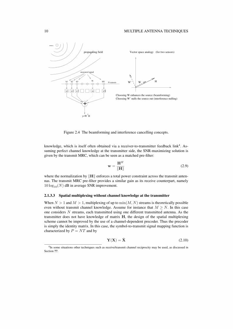
After the receiver has acquired a channel estimate (as discussed in Chapter ??), it can set thebeamforming vector w to its optimal value to maximize the received SNR. This is done byaligning the beamforming vector with the UE’s channel, via the so-called Maximum RatioCombiner (MRC) w = HH , which can be viewed as a spatial version of the well-knownmatched filter. Note that cancellation of an interfering signal can also be achieved, by se-lecting the beamforming vector to be orthogonal to the channel from the interference source.These simple concepts are illustrated vectorially in Figure 2.4.
The maximum ratio combiner provides a factor of M improvement in the received SNRcompared to the M = N = 1 case — i.e. an array gain of 10 log10(M) dB in the link budget.
In transmit beamforming, M = 1 and N > 1. The symbol-to-transmit-signal mappingfunction is characterized by P = T = 1, and Y(X) = wx, where x is the one QAM symbolto be sent. w is the transmit beamforming vector of size N × 1, computed based on channel
10 MULTIPLE ANTENNA TECHNIQUES
w1 w2 w3 wi wN
N sensorsh1 h2 h3
hihN
measured signal
+
y=W HT
source
Vector space analogy
HW’ W
propagating field
Choosing W’ nulls the source out (interference nulling)
Choosing W enhances the source (beamforming)
(for two sensors)
Figure 2.4 The beamforming and interference cancelling concepts.
knowledge, which is itself often obtained via a receiver-to-transmitter feedback link4. As-suming perfect channel knowledge at the transmitter side, the SNR-maximizing solution isgiven by the transmit MRC, which can be seen as a matched pre-filter:
w =HH
‖H‖(2.9)
where the normalization by ‖H‖ enforces a total power constraint across the transmit anten-nas. The transmit MRC pre-filter provides a similar gain as its receive counterpart, namely10 log10(N) dB in average SNR improvement.
2.1.3.3 Spatial multiplexing without channel knowledge at the transmitter
When N > 1 and M > 1, multiplexing of up to min(M,N) streams is theoretically possibleeven without transmit channel knowledge. Assume for instance that M ≥ N . In this caseone considers N streams, each transmitted using one different transmitted antenna. As thetransmitter does not have knowledge of matrix H, the design of the spatial multiplexingscheme cannot be improved by the use of a channel-dependent precoder. Thus the precoderis simply the identity matrix. In this case, the symbol-to-transmit signal mapping function ischaracterized by P = NT and by
Y(X) = X (2.10)
4In some situations other techniques such as receive/transmit channel reciprocity may be used, as discussed inSection ??.
MULTIPLE ANTENNA TECHNIQUES 11
At the receiver, a variety of linear and non-linear detection techniques may be implementedto recover the symbol matrix X. A low-complexity solution is offered by the linear case,whereby the receiver superposes N beamformers w1, w2, . . . , wN .
The detection of stream [xi, xi+N , . . . , x(N−1)T+i] is achieved by applying wi as fol-lows:
wiR = wiHX + wiN (2.11)
The design criterion for the beamformer wi can be interpreted as a compromise betweensingle-stream beamforming and cancelling of interference (created by the other N − 1 streams).Inter-stream interference is fully cancelled by selecting the Zero-Forcing (ZF) receiver givenby
W =
w1
w2
...wN
= (HHH)−1HH (2.12)
However, for optimal performance, wi should strike a balance between alignment withrespect to hi and orthogonality with respect to all other signatures hk, k 6= i. Such a balanceis achieved by, for example, a Minimum Mean-Square Error (MMSE) receiver.
Beyond classical linear detection structures such as the ZF or MMSE receivers, moreadvanced but non-linear detectors can be exploited which provide a better error rate perfor-mance at the chosen SNR operating point, at the cost of extra complexity. Examples of suchdetectors include the Successive Interference Cancelling (SIC) detector and the MaximumLikelihood Detector (MLD). The principle of the SIC detector is to treat individual streams,which are channel-encoded, like layers which are peeled off one by one by a processing se-quence consisting of linear-detection, decoding, re-modulating, re-encoding and subtractionfrom the total received signal R. On the other hand, the MLD attempts to select the mostlikely set of all streams, simultaneously, from R, by an exhaustive search procedure or alower-complexity equivalent such as the sphere-decoding technique [10].
Multiplexing gain The multiplexing gain corresponds to the multiplicative factor by whichthe spectral efficiency is increased by a given scheme. Perhaps the single most importantrequirement for MIMO multiplexing gain to be achieved is for the various transmit and re-ceive antennas to experience a sufficiently different channel response. This translates intothe condition that the spatial signatures of the various transmitters (the hi’s) (or receivers)be sufficiently decorrelated and linearly independent to allow for the channel matrix H tobe invertible (or more generally, well-conditioned). An immediate consequence of this con-dition is the limitation to min(M,N) of the number of independent streams which may bemultiplexed into the MIMO channel, or more generally to rank(H) streams. As an example,single-user MIMO communication between a four-antenna base station and a dual antennamobile UE can, at best, support multiplexing of two data streams, and thus a doubling of theUE’s data rate compared with a single stream.
2.1.3.4 Diversity
Unlike the basic multiplexing scenario in (2.10), where the design of the transmitted signalmatrix Y exhibits no redundancy between its entries, a diversity-oriented design will feature

12 MULTIPLE ANTENNA TECHNIQUES
some level of repetition between the entries of Y. For “full diversity”, each transmitted sym-bol x1 , x2 , . . . , xP must be assigned to each of the transmit antennas at least once in thecourse of the T symbol durations. The resulting symbol-to-transmit-signal mapping func-tion is called a Space-Time Block Code (STBC). Although many designs of STBC exist,additional properties such as the orthogonality of matrix Y allow improved performance andeasy decoding at the receiver. Such properties are realized by the so-called Alamouti space-time code [2], explained later in this chapter. The total diversity order which can be realizedin the N to M MIMO channel is MN when entries of the MIMO channel matrix are sta-tistically uncorrelated. The intuition behind this is that this represents the number of SISOlinks simultaneously in a state of severe fading which the system can sustain while still beingable to convey the information to the receiver. The diversity order is equal to this numberplus one. As in the previous simple multiplexing scheme, an advantage of diversity-orientedtransmission is that the transmitter does not need knowledge of the channel H, and thereforeno feedback of this parameter is necessary.
Diversity versus multiplexing trade-off A fundamental aspect of the benefits of MIMOlies in the fact that any given multiple antenna configuration has a limited number of de-grees of freedom. Thus there exists a compromise between reaching full beamforming gainin the detection of a desired stream of data and the perfect cancelling of undesired, interfer-ing streams. Similarly, there exists a trade-off between the number of streams that may bemultiplexed across the MIMO channel and the amount of diversity that each one of them willenjoy. Such a trade-off can be formulated from an information theoretic point of view [24]. Inthe particular case of spatial multiplexing of N streams over a N to M antenna channel, withM ≥ N , and using a linear detector, it can be shown that each stream will enjoy a diversityorder M −N + 1.
To some extent, increasing the spatial load of MIMO systems (i.e. the number of spatially-multiplexed streams) is akin to increasing the user load in CDMA systems. This correspon-dence extends to the fact that an optimal load level exists for a given target error rate in bothsystems.
2.1.4 Multi-user techniques2.1.4.1 Comparing single-user and multi-user MIMO
The set of MIMO techniques featuring data streams being communicated to (or from) anten-nas located on distinct UEs in the model is referred to as Multi-User MIMO (MU-MIMO).Although this situation is just as well described by our model in Equation (2.1), the MU-MIMO scenario differs in a number of crucial ways from its single-user counterpart. We firstexplain these differences qualitatively, and then present a brief survey of the most importantMU-MIMO transmission techniques.
In MU-MIMO, K UEs are selected for simultaneous communication over the same time-frequency resource, from a set of U active UEs in the cell. Typically K is much smaller thanU . Each UE is assumed to be equipped with J antennas, so the selected UEs together form aset of M = KJ UE-side antennas. Since the number of streams that may be communicatedover an N to M MIMO channel is limited to min(M,N) (if complete interference suppres-sion is intended using linear combining of the antennas), the upper bound on the number of
MULTIPLE ANTENNA TECHNIQUES 13
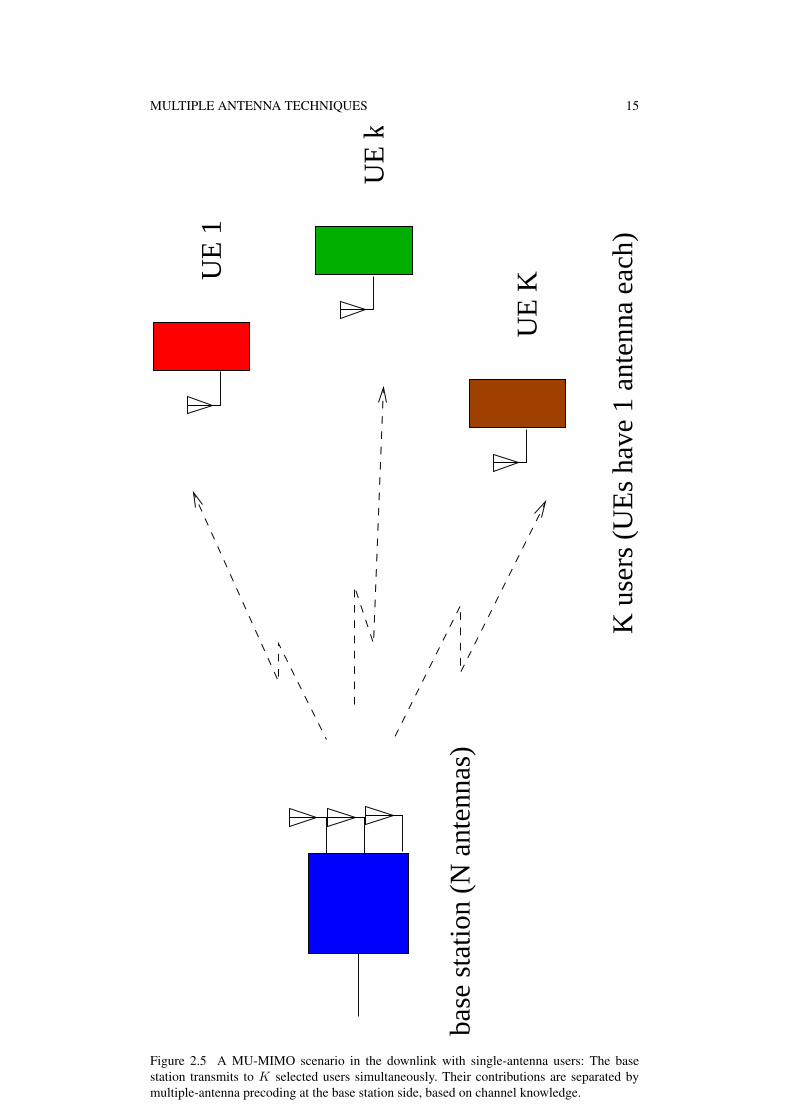
streams in MU-MIMO is typically dictated by the number of base station antennas N . Thenumber of streams which may be allocated to each UE is limited by the number of antennasJ at that UE. For instance, with single-antenna UEs, up to N streams can be multiplexed,with a distinct stream being allocated to each UE. This is in contrast to SU-MIMO, wherethe transmission of N streams necessitates that the UE be equipped with at least N antennas.Therefore a great advantage of MU-MIMO over SU-MIMO is that the MIMO multiplexingbenefits are preserved even in the case of low cost UEs with a small number of antennas. As aresult, it is generally assumed that in MU-MIMO it is the base station which bears the burdenof spatially separating the UEs, be it on the uplink or the downlink. Thus the base stationperforms receive beamforming from several UEs on the uplink and transmit beamformingtowards several UEs on the downlink.
Another fundamental contrast between SU-MIMO and MU-MIMO comes from the dif-ference in the underlying channel model. While in SU-MIMO the decorrelation between thespatial signatures of the antennas requires rich multipath propagation or the use of orthogo-nal polarizations, in MU-MIMO the decorrelation between the signatures of the different UEsoccurs naturally due to fact that the separation between such UEs is typically large relativeto the wavelength.
2.1.4.2 Techniques for single-antenna UEs
In considering the case of MU-MIMO for single-antenna UEs, it is worth noting that the num-ber of antennas available to a UE for transmission is typically less than the number availablefor reception. We therefore examine first the uplink scenario, followed by the downlink.
With a single antenna at each UE, the MU-MIMO uplink scenario is very similar to theone described by Equation (2.10): because the UEs in mobile communication systems such asLTE typically cannot cooperate and do not have knowledge of the uplink channel coefficients,no precoding can be applied and each UE simply transmits an independent message. Thus,if K users are selected for transmission in the same time-frequency resource, each user ktransmitting symbol sk, the received signal at the base station, over a single T = 1 symbolperiod, is written:
R = HX + N (2.13)
where
X =
x1
...xK
(2.14)
In this case, the columns of H correspond to the receive spatial signatures of the differentusers. The base station can recover the transmitted symbol information by applying beam-forming filters, for example using MMSE or ZF solutions (as in Equation (2.12). Note that nomore than N users can be served (i.e. K ≤ N ) if inter-user interference is to be suppressedfully.
MU-MIMO in the uplink is sometimes referred to as “Virtual MIMOŠŠ, as from the pointof view of a given UE there is no knowledge of the simultaneous transmissions of the otherUEs. This transmission mode and its implications for LTE are discussed in Section ??.
On the downlink, which is illustrated in Figure 2.5, the base station must resort to transmitbeamforming in order to separate the data streams intended for the various UEs. Over a single

14 MULTIPLE ANTENNA TECHNIQUES
T = 1 symbol period, the signal received by UEs 1 to K can be written compactly as
R =
r1
...rK
= HVPX + N (2.15)
This time, the rows of H correspond to the transmit spatial signatures of the various UEs. Vis the transmit beamforming matrix and P is the (diagonal) power allocation matrix selectedsuch that it fulfils the total normalized transmit power constraint Pt. To cancel out fully theinter-user interference when K ≤ N , a transmit ZF beamforming solution may be employed(although this is not optimal due to the fact that it may require a high transmit power if thechannel is ill-conditioned). Such a solution would be given by:
V = HH(HHH)−1 (2.16)
Note that regardless of the channel realization, the power allocation must be chosen to satisfyany power constraints at the base station, for example such that trace(VPPHVH) = Pt.
2.1.4.3 Techniques for multiple-antenna UEs
The ideas presented above for single antenna UEs can be generalized to the case of multipleantenna UEs. There could, in theory, be essentially two ways of exploiting the additionalantennas at the UE side. In the first approach, the multiple antennas are simply treated asmultiple virtual UEs, allowing high-capability terminals to receive or transmit more than onestream, while at the same time spatially sharing the channel with other UEs. For instance, afour antenna base station could theoretically communicate in a MU-MIMO fashion with twoUEs equipped with two antennas each, allowing two streams per UE, resulting in a total mul-tiplexing gain of four. Another example would be that of two single-antenna UEs, receivingone stream each, and sharing access with another two-antenna UE, the latter receiving twostreams. Again the overall multiplexing factor remains limited to the number of base stationantennas.
The second approach for making use of additional UE antennas is to treat them as extradegrees of freedom for the purpose of strengthening the link between the UE and the basestation. Multiple antennas at the UE may then be combined in MRC fashion in the case of thedownlink, or in the case of the uplink space-time coding could be used. Antenna selection isanother way of extracting more diversity out of the channel, as discussed in Section ??.
2.1.4.4 Comparing single-user and multi-user capacity
To illustrate the gains of multi-user multiplexing over single-user transmission, we comparethe sum-rate achieved by both types of system from an information theoretic standpoint, forsingle antenna UEs. We compare the Shannon capacity in single-user and multi-user scenar-ios both for an idealized synthetic channel and for a channel obtained from real measurementdata.
The idealized channel model assumes that the entries of the channel matrix H in Equation (2.13)are identically and independently distributed (i.i.d.) Rayleigh fading. For the measured chan-nel case, a channel sounder was used 5 to perform real-time wideband channel measurements
5The Eurecom MIMO OpenAir Sounder (EMOS) [17]
MULTIPLE ANTENNA TECHNIQUES 15
UE
k
UE
K
UE
1
base
sta
tion
(N a
nten
nas)
K u
sers
(U
Es
have
1 a
nten
na e
ach)
Figure 2.5 A MU-MIMO scenario in the downlink with single-antenna users: The basestation transmits to K selected users simultaneously. Their contributions are separated bymultiple-antenna precoding at the base station side, based on channel knowledge.

16 MULTIPLE ANTENNA TECHNIQUES
Table 2.1 Parameters of the measured channel for SU-MIMO /MU-MIMO comparison. More details can be found in [17, 18].
Parameter Value
Centre Frequency 1917.6 MHzBandwidth 4.8 MHzBase Station Transmit Power 30 dBmNumber of Antennas at Base Station 4 (2 cross polarized)Number of UEs 2Number of Antennas at UE 1Number of Sub-carriers 160
synchronously for two UEs moving at vehicular speed in an outdoor semi-urban hilly en-vironment with LOS propagation predominantly present. The most important parameters ofthe platform are summarized in Table 2.1.
We compare the sum rate capacity of a two-UE MIMO system (calculated assuminga zero-forcing precoder as described in Section 2.1.4) with the capacity of an equivalentMISO system serving a single UE at a time (i.e. in TDMA), employing beamforming (seeSection 2.1.3.2). The base has four antennas and the UE has a single antenna. Full ChannelState Information at the Transmitter (CSIT) is assumed in both cases.
Figure 2.6 shows the ergodic (mean) sum rate of both schemes in both channels. Themean is taken over all frames and all sub-carriers and subsequently normalized to bits/sec/Hz.It can be seen that in both the ideal and the measured channels, MU-MIMO yields a highersum rate than SU-MISO in general. In fact, at high SNR, the multiplexing gain of the MU-MIMO system is two while it is limited to one for the SU-MISO case.
However, for low SNR, the SU-MISO TDMA and MU-MIMO schemes perform verysimilarly. This is because a sufficient SNR is required to excite more than one MIMO trans-mission mode. Interestingly, the performance of both SU-MISO TDMA and MU-MIMO isslightly worse in the measured channels than in the idealized i.i.d. channels. This can beattributed to the correlation of the measured channel in time (due to the relatively slow move-ment of the users), in frequency (due to the Line Of Sight (LOS) propagation), and in space(due to the transmit antenna correlation). In the MU-MIMO case the difference between thei.i.d. and the measured channel is much stronger than in the single-user TDMA case, sincethese correlation effects result in a rank-deficient channel matrix.
2.2 MIMO schemes in LTEBuilding on the theoretical background of the previous section, the MIMO schemes adoptedfor LTE are reviewed and explained. These schemes relate to the downlink unless otherwisementioned.
2.2.1 Practical considerationsWe first review briefly a few important practical constraints which affect the real-life per-formance of the theoretical MIMO systems considered above, and which often are decisive

MULTIPLE ANTENNA TECHNIQUES 17
−20 −15 −10 −5 0 5 10 15 20 25 300
2
4
6
8
10
12
14
16
18
SNR [dB]
Su
m r
ate
[bit
s/se
c/H
z]
MU−MIMO ZF iidSU−MISO TDMA iidMU−MIMO ZF measSU−MISO TDMA meas
Figure 2.6 Ergodic sum rate capacity of SU-MISO TDMA and MU-MIMO with 2 UEs, foran i.i.d. Rayleigh fading channel and for a measured channel.
18 MULTIPLE ANTENNA TECHNIQUES
when selecting a particular transmission strategy in a given propagation and system setting.It was argued above that the full MIMO benefits (array gain, diversity gain and multi-
plexing gain) assume ideally decorrelated antennas and full-rank MIMO channel matrices.In this regard, the propagation environment and the antenna design (e.g. the spacing) play asignificant rôle. In the single-user case, the antennas at both the base station and the UE aretypically separated by between half a wavelength and a couple of wavelengths at most. Thisdistance is very short in relation with the distance from base statio to UE. In a LOS situa-tion, this will cause a strong correlation between the spatial signatures, limiting the use ofmultiplexing schemes. However, an exception to this can be created from the use of antennaswhose design itself provides the necessary orthogonality properties even in LOS situations.An example is the use of two antennas (at both transmitter and receiver), which operateon orthogonal polarizations (e.g. horizontal and vertical polarizations, or better, so-called+45◦ and −45◦ polarizations, which give a two-fold multiplexing capability even in LOS).However the use of orthogonal polarizations at the UEs may not always be recommendedas it results in non-omnidirectionnal beam patterns. Such exceptions aside, in single-userMIMO the condition of spatial signature independence can only be satisfied with the helpof rich random multipath propagation. In diversity-oriented schemes, the invertibility of thechannel matrix is not required, yet the entries of the channel matrix should be statisticallydecorrelated. Although a greater LOS to non-LOS energy ratio will tend to correlate the fad-ing coefficients on the various antennas, this effect will be compensated by the reduction infading delivered by the LOS component.
Another source of discrepancy between theoretical MIMO gains and practically-achievedperformance lies in the (in-)ability of the receiver, and whenever needed the transmitter, toestimate the channel coefficients perfectly. At the receiver, channel estimation is typicallyperformed over a finite sample of Reference Symbols (RS), as discussed in Chapter ??. Inthe case of transmit beamforming and MIMO SVD-based precoding, the transmitter then hasto acquire this channel knowledge (or directly the precoder knowledge) from the receiverusually through a limited feedback link, which causes further degradation to the availableChannel State Information at the Transmitter (CSIT).
When it comes to MU-MIMO, the principle advantages over SU-MIMO are clear: robust-ness with respect to the propagation environment, and spatial multiplexing gain preservedeven in the case of UEs with small numbers of antennas. However, such advantages come ata price. In the downlink, MU-MIMO relies on the ability of the base station to compute therequired transmit beamformer, which in turn requires CSIT. The fundamental role of CSITin the MU-MIMO downlink can be emphasized as follows: in the extreme case of no CSITbeing available and identical fading statistics for all the UEs, the MU-MIMO gains totallydisappear and the SU-MIMO strategy becomes optimal [4].
As a consequence, one of the most difficult challenges in making MU-MIMO practicalfor cellular applications, and particularly for an FDD system, is devising mechanisms thatallow for accurate CSI to be delivered by the UE to the base station in a resource-efficientmanner. This requires the use of appropriate codebooks for quantization. These aspects aredeveloped later in this chapter. A recent account of the literature on this subject may also befound in [12].
Another issue which arises for practical implementations of MIMO schemes is the inter-action between the physical layer and the scheduling protocol. As noted in Section 2.1.4.1,in both uplink and downlink cases the number of UEs which can be served in a MU-MIMO
MULTIPLE ANTENNA TECHNIQUES 19
fashion is typically limited to K = N , assuming linear combining structures. Often one mayeven decide to limit K to a value strictly less than N to preserve some degrees of freedomfor per-user diversity. As the number of active users U will typically exceed K, a selectionalgorithm must be implemented to identify which set of users will be scheduled for simul-taneous transmission over a particular time-frequency slot. This algorithm is not specified inLTE and various approaches are possible; as discussed in Chapter ??, a combination of ratemaximization and QoS constraints will typically be considered. It is important to note thatthe choice of UEs that will maximize the sum rate (the sum over the K individual rates fora given subframe) is one that favours UEs exhibiting not only good instantaneous SNR butalso spatial separability among their signatures.
2.2.2 Single-user schemes
In this section, we examine the solutions adopted in LTE for SU-MIMO. We consider firstthe diversity schemes used on the transmit side, then beamforming schemes, and finally welook at the spatial multiplexing mode of transmission.
2.2.2.1 Transmit diversity schemes
The theoretical aspects of transmit diversity were discussed in Section 2.1. Here we discussthe two main transmit diversity techniques defined in LTE. In LTE, transmit diversity is onlydefined for 2 and 4 transmit antennas, and one data stream, referred to in LTE as one code-word since one transport block CRC is used per data stream. To maximize diversity gain theantennas typically need to be uncorrelated, so they need to be well separated relative to thewavelength or have different polarization. Transmit diversity still has its value in a number ofscenarios, including low SNR, low mobility (no time diversity), or for applications with lowdelay tolerance. Diversity schemes are also desirable for channels for which no UL feedbacksignalling is available (e.g. Multimedia Broadcast Multicast Services (MBMS) described inChapter ??, Physical Broadcast Channel (PBCH) in Chapter ?? and Synchronization Signalsin Chapter ??).
In LTE the MIMO scheme is independently assigned for the control channels and thedata channels, and is also assigned independently per UE in the case of the data channels(Physical Downlink Shared CHannel — PDSCH).
In this section we will discuss in more detail the transmit diversity techniques of SpaceFrequency Block Codes (SFBC) and Frequency Switched Transmit Diversity (FSTD), aswell as the combination of these schemes as used in LTE. These transmit diversity schemesmay be used in LTE for the PBCH and Physical Downlink Control Channel (PDCCH), andalso for the PDSCH if it is configured in transmit diversity mode6 for a UE.
Another transmit diversity technique which is commonly associated with OFDM is CyclicDelay Diversity (CDD). CDD is not used in LTE as a diversity scheme in its own right butrather as a precoding scheme for spatial multiplexing on the PDSCH; we therefore introduceit later in Section 2.2.2.3 in the context of spatial multiplexing.
6PDSCH Transmission Mode 2 — see Section ??
20 MULTIPLE ANTENNA TECHNIQUES
Space Frequency Block Codes (SFBC) If a physical channel in LTE is configured forTransmit Diversity operation using two eNodeB antennas, SFBC is used. SFBC is a frequency-domain version of the well-known Space-Time Block Codes (STBC), also known as Alam-outi codes [2]. This family of codes is designed so that the transmitted diversity streams areorthogonal and achieve the optimal SNR with a linear receiver. Such orthogonal codes onlyexist for the case of two transmit antennas.
STBC is used in UMTS, but in LTE the number of available OFDM symbols in a sub-frame is often odd while STBC operates on pairs of adjacent symbols in the time domain. Theapplication of STBC is therefore not straightforward for LTE, while the multiple sub-carriersof OFDM lend themselves well to the application of SFBC.
For SFBC transmission in LTE, the symbols transmitted from the two eNodeB antennaports on each pair of adjacent sub-carriers are defined as follows:[
y(0)(1) y(0)(2)y(1)(1) y(1)(2)
]=
[x1 x2
−x∗2 x∗1
](2.17)
where y(p)(k) denotes the symbols transmitted from antenna port p on the kth subcarrier.Since no orthogonal codes exist for antenna configurations beyond 2× 2, SFBC has to
be modified in order to apply it to the case of 4 transmit antennas. In LTE, this is achieved bycombining SFBC with Frequency-Switched Transmit Diversity (FSTD).
Frequency Switched Transmit Diversity (FSTD) and its combination with SFBC Gen-eral FSTD schemes transmit symbols from each antenna on a different set of subcarriers. Forexample, an FSTD transmission from 4 transmit antennas on four subcarriers might appearas follows:
y(0)(1) y(0)(2) y(0)(3) y(0)(4)y(1)(1) y(1)(2) y(1)(3) y(1)(4)y(2)(1) y(2)(2) y(2)(3) y(2)(4)y(3)(1) y(3)(2) y(3)(3) y(3)(4)
=
x1 0 0 00 x2 0 00 0 x3 00 0 0 x4
(2.18)
where, as previously, y(p)(k) denotes the symbols transmitted from antenna port p on the kth
subcarrier. In practice in LTE, FSTD is only used in combination with SFBC for the caseof 4 transmit antennas, in order to provide a suitable transmit diversity scheme where noorthogonal rate 1 block codes exists. The LTE scheme is in fact a combination of two 2× 2SFBC schemes mapped to independent sub-carriers as follows:
y(0)(1) y(0)(2) y(0)(3) y(0)(4)y(1)(1) y(1)(2) y(1)(3) y(1)(4)y(2)(1) y(2)(2) y(2)(3) y(2)(4)y(3)(1) y(3)(2) y(3)(3) y(3)(4)
=
x1 x2 0 00 0 x3 x4
−x∗2 x∗1 0 00 0 −x∗4 x∗3
(2.19)
Note that mapping of symbols to antenna ports is different in the 4 transmit antenna casecompared to the 2 transmit-antenna SFBC scheme. This is because the RS density on the thirdand fourth antenna ports is half that of the first and second antenna ports (see Section ??), andhence the channel estimation accuracy may be lower on the third and fourth antenna ports.Thus this design of the transmit diversity scheme avoids concentrating the channel estimationlosses in just one of the SFBC codes, resulting in a slight coding gain.

MULTIPLE ANTENNA TECHNIQUES 21
2.2.2.2 Beamforming schemes
The theoretical aspects of beamforming were described in Section 2.1. Here we explain howit is implemented in LTE.
LTE differentiates between two transmission modes which may support beamforming forthe PDSCH:
• Closed-loop rank 1 precoding7. Although this amounts to beamforming, it can alsobe seen as a special case of SU-MIMO spatial multiplexing and is therefore discussedin Section 2.2.2.3. In this mode the UE feeds channel information back to the eNodeBto indicate suitable precoding to apply for the beamforming operation.
• UE-specific RSs8. In this mode the UE does not feed back any precoding-related in-formation. The eNodeB instead tries to deduce this information, for example usingDirection Of Arrival (DOA) estimations from the uplink, in which case it is worthnoting that calibration of the eNodeB RF paths may be necessary, as discussed inSection ??.
In this section we focus on the latter case. This mode is primarily a mechanism to extendcell coverage by concentrating the eNodeB power in the direction in which the UE is located.It typically has the following properties:
• It can conveniently be implemented by an array of closely-spaced antenna elements forcreating directional transmissions. The signals from the different antenna elements arephased to all arrive in phase in the desired direction for the UE.
• The eNodeB is responsible for ensuring that the beam is correctly directed, as the UEdoes not explicitly indicate a preference regarding the direction/selection of the beam.
• Other than being directed to use the UE-specific RS as the phase reference, a UE wouldnot really be aware that it is receiving a directional transmission rather than a cell-wide transmission. To the UE, the phased array of antenna ports “appears” as just oneantenna.
One side-effect of using beamforming based on UE-specific RS is that channel qualityexperienced by the UE will typically be different (hopefully better) than that of any of thecommon RS. However, as the UE-specific RS are only provided in the specific RBs for whichthe beamforming transmission mode is applied, the eNodeB cannot rely on the UE beingable to derive Channel Quality Indicator (CQI) feedback from the UE-specific RS. For thisreason, it is specified in LTE that CQI feedback from a UE configured with UE-specificRS is derived using the common RS transmitted on the first antenna port (“antenna port0”). This suggests a deployment scenario whereby antenna port 0 actually uses one of theelements of the phased array. The eNodeB could then, over time, establish a suitable offsetto apply to the CQI reports received from the UE to adapt them to the actual quality of thebeamformed signal. Such an offset might, for example, be derived from the proportion oftransport blocks positively acknowledged by the UE. An eNodeB antenna configuration ofthis kind also allows the possibility to use beamforming for UEs near the edge of the cell,
7PDSCH transmission mode 6 — see Section ??8PDSCH transmission mode 7 — see Section ??

22 MULTIPLE ANTENNA TECHNIQUES
while other antenna ports may be used for SU-MIMO spatial multiplexing to deliver highdata rates to UEs clser to the eNodeB.
Another factor to consider when deploying beamforming in LTE is that it can only beapplied to the PDSCH and not to the control channels. Typically the range of the PDSCHcan therefore be extended by beamforming, but the overall cell range may still be limited bythe range of the control channels unless other measures are taken. One approach could beto reduce the code rate used for the control channels when beamforming is applied to thePDSCH.
The effect of beamforming on neighbouring cells should also be taken into account. If thebeamforming is intermittent, it can result in a problem often known as the “flash light effect”,where strong intermittent interference may disturb the accuracy of the UEs’ CQI reportingin adjacent cells. This effect was shown to have the potential to cause throughput reductionsin HSDPA [22], but in LTE the possibility for frequency-domain scheduling in OFDMA (asdiscussed in Section ??) provides an additional degree of freedom to avoid such issues.
2.2.2.3 Spatial multiplexing schemes
Introduction We begin by introducing some terminology used to describe spatial multi-plexing in LTE:
• A spatial layer is the term used in LTE for the different streams generated by spa-tial multiplexing as described in Section 2.1. A layer can be described as a mappingof symbols onto the transmit antenna ports. Each layer is identified by a (precoding)vector of size equal to the number of transmit antennas and can be associated with aradiation pattern.
• The rank of the transmission is the number of layers transmitted.
• A codeword is an independently encoded data block, corresponding to a single Trans-port Block delivered from the MAC layer in the transmitter to the physical layer fortransmission, and protected with a CRC.
For ranks greater than 1, two codewords can be transmitted. Note that the number ofcodewords is always less than or equal to the number of layers, which in turn is always lessthan or equal to the number of antenna ports.
In principle, a SU-MIMO spatial multiplexing scheme can either use a single codewordmapped to all the available layers, or multiple codewords each mapped to one or more differ-ent layers.
The main benefit of using only one codeword is a reduction in the amount of controlsignalling required, both for CQI reporting, where only a single value would be needed forall layers, and for HARQ ACK/NACK feedback, where only one ACK/NACK would haveto be signalled per subframe per UE. In such a case, the MLD receiver is optimal in terms ofminimizing the bit error rate.
At the opposite extreme, a separate codeword could be mapped to each of the layers.The advantage of this type of scheme is that significant gains are possible from Succes-sive Interference Cancellation (SIC), albeit at the expense of more signalling being required.An MMSE-SIC receiver can be shown to achieve the Shannon capacity [?]. Note that an
MULTIPLE ANTENNA TECHNIQUES 23
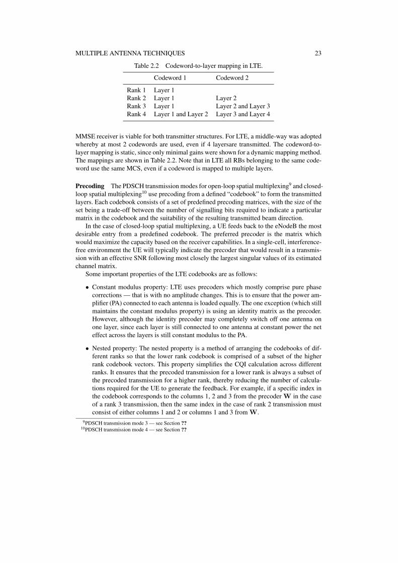
Table 2.2 Codeword-to-layer mapping in LTE.
Codeword 1 Codeword 2
Rank 1 Layer 1Rank 2 Layer 1 Layer 2Rank 3 Layer 1 Layer 2 and Layer 3Rank 4 Layer 1 and Layer 2 Layer 3 and Layer 4
MMSE receiver is viable for both transmitter structures. For LTE, a middle-way was adoptedwhereby at most 2 codewords are used, even if 4 layersare transmitted. The codeword-to-layer mapping is static, since only minimal gains were shown for a dynamic mapping method.The mappings are shown in Table 2.2. Note that in LTE all RBs belonging to the same code-word use the same MCS, even if a codeword is mapped to multiple layers.
Precoding The PDSCH transmission modes for open-loop spatial multiplexing9 and closed-loop spatial multiplexing10 use precoding from a defined “codebook” to form the transmittedlayers. Each codebook consists of a set of predefined precoding matrices, with the size of theset being a trade-off between the number of signalling bits required to indicate a particularmatrix in the codebook and the suitability of the resulting transmitted beam direction.
In the case of closed-loop spatial multiplexing, a UE feeds back to the eNodeB the mostdesirable entry from a predefined codebook. The preferred precoder is the matrix whichwould maximize the capacity based on the receiver capabilities. In a single-cell, interference-free environment the UE will typically indicate the precoder that would result in a transmis-sion with an effective SNR following most closely the largest singular values of its estimatedchannel matrix.
Some important properties of the LTE codebooks are as follows:
• Constant modulus property: LTE uses precoders which mostly comprise pure phasecorrections — that is with no amplitude changes. This is to ensure that the power am-plifier (PA) connected to each antenna is loaded equally. The one exception (which stillmaintains the constant modulus property) is using an identity matrix as the precoder.However, although the identity precoder may completely switch off one antenna onone layer, since each layer is still connected to one antenna at constant power the neteffect across the layers is still constant modulus to the PA.
• Nested property: The nested property is a method of arranging the codebooks of dif-ferent ranks so that the lower rank codebook is comprised of a subset of the higherrank codebook vectors. This property simplifies the CQI calculation across differentranks. It ensures that the precoded transmission for a lower rank is always a subset ofthe precoded transmission for a higher rank, thereby reducing the number of calcula-tions required for the UE to generate the feedback. For example, if a specific index inthe codebook corresponds to the columns 1, 2 and 3 from the precoder W in the caseof a rank 3 transmission, then the same index in the case of rank 2 transmission mustconsist of either columns 1 and 2 or columns 1 and 3 from W.
9PDSCH transmission mode 3 — see Section ??10PDSCH transmission mode 4 — see Section ??

24 MULTIPLE ANTENNA TECHNIQUES
• Minimal “complex” multiplications: The 2-antenna codebook consists entirely of aQPSK alphabet, which eliminates the need for any complex multiplications since allcodebook multiplications use only ±1 and ±j. The 4-antenna codebook does containsome 8PSK entries which require a
√2 magnitude scaling as well; it was considered
that the performance gain of including these precoders justified the added complexity.
The 2-antenna codebook in LTE is comprised of one 2× 2 identity matrix and two DFTmatrices: [
1 00 1
],
[1 11 −1
]and
[1 1j −j
](2.20)
Here the columns of the matrices correspond to the layers.The four transmit antenna codebook in LTE uses a Householder generating function:
WH = I− 2uuH/uHu, (2.21)
which generates unitary matrices from input vectors u, which are defined in [1]. The advan-tage of using precoders generated with this equation is that it simplifies the CQI calculation(which has to be carried out for each individual precoder in order to determine the pre-ferred precoder) by reducing the number of matrix inversions. This structure also reduces theamount of control signalling required, since the optimum rank 1 version of WH is always thefirst column of WH ; therefore the UE only needs to indicate the preferred precoding matrix,and not also the individual vector within it which would be optimal for the case of rank 1transmission.
Note that both DFT and Householder matrices are unitary.
Cyclic Delay Diversity (CDD) In the case of open-loop spatial multiplexing11, the feed-back from the UE indicates only the rank of the channel, and not a preferred precodingmatrix. In this mode, if the rank used for PDSCH transmission is greater than 1 (i.e. morethan one layer is transmitted), LTE uses Cyclic Delay Diversity (CDD) [?]. CDD involvestransmitting the same set of OFDM symbols on the same set of OFDM sub-carriers frommultiple transmit antennas, with a different delay on each antenna. The delay is applied be-fore the cyclic prefix (CP) is added, thereby guaranteeing that the delay is cyclic over theFFT size. This gives CDD its name.
Adding a time delay is identical to applying a phase shift in the frequency domain. As thesame time delay is applied to all sub-carriers, the phase shift will increase linearly across thesub-carriers with increasing sub-carrier frequency. Each sub-carrier will therefore experiencea different beamforming pattern as the non-delayed subcarrier from one antenna interferesconstructively or destructively with the delayed version from another antenna. The diversityeffect of CDD therefore arises from the fact that different sub-carriers will pick out differentspatial paths in the propagation channel, thus increasing the frequency-selectivity of the chan-nel. The channel coding, which is applied to a whole transport block across the sub-carriers,ensures that the whole transport block benefits from the diversity of spatial paths.
Although this approach does not optimally exploit the channel in the way that ideal pre-coding would (by matching the precoding to the eigenvectors of the channel), it does help toensure that any destructive fading is constrained to individual sub-carriers rather than affect-ing a whole transport block. This can be particularly beneficial if the channel information at
11PDSCH transmission mode 3
MULTIPLE ANTENNA TECHNIQUES 25
the transmitter is unreliable, for example due to the feedback being limited or the UE velocitybeing high.
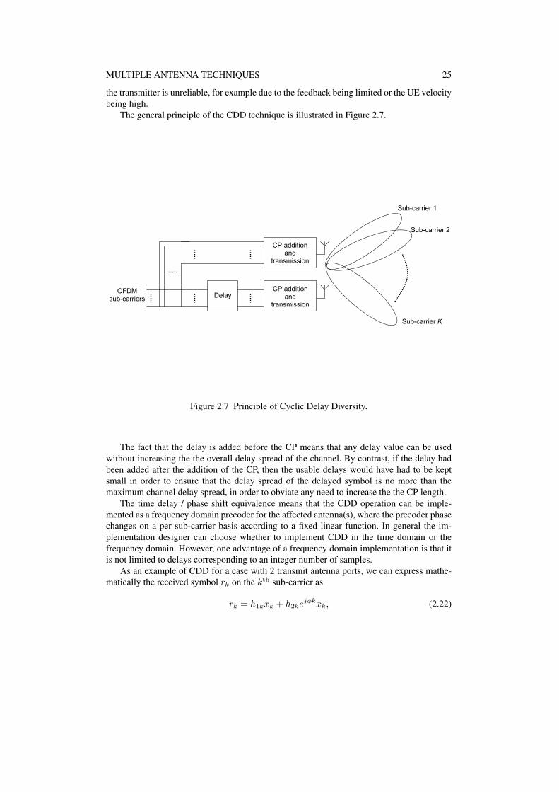
The general principle of the CDD technique is illustrated in Figure 2.7.
Delay OFDM sub-carriers
CP addition and
transmission
CP addition and
transmission
Sub-carrier 1
Sub-carrier 2
Sub-carrier K
Figure 2.7 Principle of Cyclic Delay Diversity.
The fact that the delay is added before the CP means that any delay value can be usedwithout increasing the the overall delay spread of the channel. By contrast, if the delay hadbeen added after the addition of the CP, then the usable delays would have had to be keptsmall in order to ensure that the delay spread of the delayed symbol is no more than themaximum channel delay spread, in order to obviate any need to increase the the CP length.
The time delay / phase shift equivalence means that the CDD operation can be imple-mented as a frequency domain precoder for the affected antenna(s), where the precoder phasechanges on a per sub-carrier basis according to a fixed linear function. In general the im-plementation designer can choose whether to implement CDD in the time domain or thefrequency domain. However, one advantage of a frequency domain implementation is that itis not limited to delays corresponding to an integer number of samples.
As an example of CDD for a case with 2 transmit antenna ports, we can express mathe-matically the received symbol rk on the kth sub-carrier as
rk = h1kxk + h2kejφkxk, (2.22)
26 MULTIPLE ANTENNA TECHNIQUES
where hpk is the channel from the pth transmit antenna, and ejφk is the phase shift on thekth sub-carrier due to the delay operation. We can see clearly that on some sub-carriers thesymbols from the second transmit antenna will add constructively, while on other sub-carriersthey will add destructively. Here, φ = 2πdcdd/N , where N is the FFT size and dcdd is thedelay in samples.
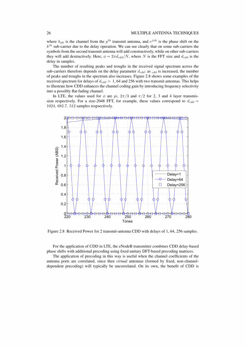
The number of resulting peaks and troughs in the received signal spectrum across thesub-carriers therefore depends on the delay parameter dcdd: as cdd is increased, the numberof peaks and troughs in the spectrum also increases. Figure 2.8 shows some examples of thereceived spectrum for delays of dcdd = 1, 64 and 256 with two transmit antennas. This helpsto illustrate how CDD enhances the channel coding gain by introducing frequency selectivityinto a possibly flat-fading channel.
In LTE, the values used for φ are pi, 2π/3 and π/2 for 2, 3 and 4 layer transmis-sion respectively. For a size-2048 FFT, for example, these values correspond to dcdd =1024, 682.7, 512 samples respsectively.
220 230 240 250 260 270 2800
0.2
0.4
0.6
0.8
1
1.2
1.4
1.6
1.8
2
Tones
Rec
eive
d P
ower
(AB
S)
Delay=1Delay=64Delay=256
Figure 2.8 Received Power for 2 transmit-antenna CDD with delays of 1, 64, 256 samples.
For the application of CDD in LTE, the eNodeB transmitter combines CDD delay-basedphase shifts with additional precoding using fixed unitary DFT-based precoding matrices.
The application of precoding in this way is useful when the channel coefficients of theantenna ports are correlated, since then virtual antennas (formed by fixed, non-channel-dependent precoding) will typically be uncorrelated. On its own, the benefit of CDD is

MULTIPLE ANTENNA TECHNIQUES 27
reduced by antenna correlation. This can be illustrated by an extreme example with fullcorrelation:
• Assume that the two physical channels are identical, and the CDD delay is chosen suchthat at each alternate sub-carrier frequency the net combined channel is the sum of thetwo channels, and at each other alternate frequency the net combined channel is thedifference between the two physical channels:
r2k = (h1 + h2)x2k, (2.23)
r2k+1 = (h1 − h2)x2k+1, (2.24)
h1 = h2. (2.25)
Clearly, at the odd frequencies where the channels subtract, no signal will be received,and effectively the bandwidth is halved.
The use of uncorrelated virtual antennas created by fixed precoding can avoid this problemin correlated channels, while not degrading the performance if the individual antenna portsare uncorrelated.
For ease of explanation, the discussion of CDD so far has been in terms of a rank-1transmission — i.e. with a single layer. However, in practice, CDD is only applied in LTEwhen the rank used for PDSCH transmission is greater than 1. In such a case, each layerbenefits independently from CDD in the same way as for a single layer. For example, for arank 2 transmission, the transmission on the second antenna port is delayed relative to thefirst antenna port for each layer. This means that symbols transmitted on both layers willexperience the delay and hence the increased frequency selectivity.
For multi-layer CDD operation, the mapping of the layers to antenna ports is carriedout using precoding matrices selected from the spatial multiplexing codebooks describedearlier. As the UE does not indicate a preferred precoding matrix in the open loop spatialmultiplexing transmission mode in which CDD is used, the particular spatial multiplexingmatrices selected from the spatial multiplexing codebooks in this case are predetermined.
In the case of two transmit antenna ports, the predetermined spatial multiplexing precod-ing matrix W is always the same (the first entry in the two transmit antenna port codebook,which is the identity matrix). Thus the transmitted signal can be expressed as follows:[
y(0)(k)y(1)(k)
]= WD2U2x =
1√2
[1 00 1
]1√2
[1 00 ejφ1k
] [1 11 −1
] [x(0)(i)x(1)(i)
](2.26)
In the case of four transmit antenna ports, ν different precoding matrices are used fromthe four transmit antenna port codebook where ν is the transmission rank. These ν precodingmatrices are applied in turn across groups of ν sub-carriers in order to provide additionaldecorrelation between the spatial streams.
2.2.2.4 Feedback computation and signalling
In addition to CQI reporting as discussed in Section ??, to support MIMO operation the UEcan be configured to report Precoding Matrix Indicators (PMI) and Rank Indicators (RI). Theprecoding described above is applied relative to the phase of the common reference symbols

28 MULTIPLE ANTENNA TECHNIQUES
for each antenna port. Thus if the UE knows the precoding matrices that could be applicable(as defined in the configured codebook), and it knows the transfer function of the channelsfrom the different antenna ports (by making measurements on the reference symbols), it candetermine which W is most suitable under the current radio conditions and signal this to theeNodeB. The preferred W, whose index constitutes the PMI report, is the precoder whichmaximizes the aggregate number of data bits which could be received across all layers.
The UE can also be configured to report the channel rank via a RI, which is calculatedto maximize the capacity over the entire bandwidth, jointly selecting the preferred precoderper sub-band to maximize its capacity on the assumption of the selected rank. The UE alsoreports CQI values corresponding to the preferred rank and precoders, to enable the eNodeBto perform link adaptation and multi-user scheduling as discussed in Sections ?? and ??. Thenumber of CQI values reported normally corresponds to the number of codewords supportedby the preferred rank. Further, the CQI values themselves will depend on the assumed rank:for example, the precoding matrix for layer 1 will usually be different depending on whetherthe UE is assuming the presence of a second layer or not.
The eNodeB is not bound to use the precoder requested by the UE, but clearly if theeNodeB chooses another precoder then the reported CQI cannot be assumed to be valid.For each PDSCH transmission to a UE, the eNodeB indicates via the PDCCH whether it isapplying the UE’s preferred precoder, and if not, which precoder is used. This enables theUE to derive the correct phase reference relative to the common RS in order to demodulatethe PDSCH data.
The number of RBs to which each PMI corresponds in the frequency domain is config-urable by the eNodeB. A typically value is likely to be 5 RBs (900 kHz).
Although the UE indicates the rank which would maximize the downlink data rate, theeNodeB can also indicate to the UE that a different rank is being used for a PDSCH trans-mission. This gives flexibility to the eNodeB, since the UE does not know the amount of datain the downlink buffer; if the amount of data in the buffer is small, the eNodeB may prefer touse a lower rank with higher reliability.
Thus all three types of feedback — CQI, PMI and RI — are fundamental components ofmaking satisfactory practical use of the available SU-MIMO transmission techniques in theLTE downlink.
2.2.3 Multi-user schemes
MU-MIMO is the most recent aspects of MIMO technology, which has been the subjectof much interest during the development of LTE. However, MU-MIMO typically entails afairly significant change of perspective compared to other more familiar MIMO techniques.As pointed out in Section 2.2.1, the availability of accurate CSIT is the main challenge inmaking MU-MIMO schemes attractive for cellular applications. As a result, the main focusfor MIMO in the first release of LTE is on achieving transmit antenna diversity or single-usermultiplexing gain, neither of which requires such a sophisticated CSI feedback mechanism.
Thus the support for MU-MIMO in the first version of LTE is rather limited. However, itis very likely that more advanced MU-MIMO techniques will be a part of future versions ofLTE, and that more sophisticated and resource-efficient solutions for channel estimation andfeedback will play a crucial role in making these techniques a practical success.
MULTIPLE ANTENNA TECHNIQUES 29
Many variations of MU-MIMO may be considered, and the choice of a particular algo-rithm reflects a compromise between complexity, performance and the amount of feedbacknecessary to convey the CSIT to the eNodeB. In this Section we describe the main aspectsof MU-MIMO techniques which emerged during the development of LTE, with the aim ofhighlighting the available technical solutions and the challenges which remain.
2.2.3.1 Precoding strategies and supporting signalling
MU-MIMO is particularly beneficial for increasing total cell throughput in the downlink:when the eNodeB has N transmit antennas and U ≥ N UEs are present in the cell, it is wellknown that the full multiplexing gain N can be achieved even when each UE has only asingle antenna, by using SDMA (space-division multiple access) schemes based on linearprecoding for transmit beamforming. Moreover, when the number of active UEs in the cell islarge, a significant portion of the MU-MIMO throughput gain can be secured by exploitingmultiuser diversity through relatively simple UE-selection mechanisms. All these benefits,however, depend on the level of CSIT that the eNodeB receives from each UE.
In the case of SU-MIMO, and it has been shown that even a small number of feedback bitsper antenna can be very beneficial in steering the transmitted energy more accurately towardsthe UE’s antenna(s) [21, 19, 20, 16]. More precisely, in SU-MIMO channels the accuracy ofCSIT only causes an SNR offset, but does not affect the slope of the capacity-versus-SNRcurve (i.e. the multiplexing gain). Yet for the MU-MIMO downlink, the level of CSI avail-able at the transmitter does affect the multiplexing gain, because a MU-MIMO system withfinite-rate feedback is essentially interference-limited, where the crucial interference rejec-tion processing is carried out by the transmitter. Hence, providing accurate channel feedbackis considerably more important for MU-MIMO than for SU-MIMO.
On the other hand, in a system with a large number of UEs, if all the UEs are to reportvery accurate channel measurements, the total amount of uplink resources required for CSITfeedback may soon outweigh the increase in system throughput provided by MU-MIMOtechniques. Recent published results show that, given a total feedback budget, considerablyhigher throughput is achieved by receiving very accurate channel feedback from a relativelysmall fraction of the UEs, selected according to some appropriate criterion, rather than coarsefeedback from many UEs [27].
One general solution to the problem of limited CSIT feedback in MU-MIMO schemesis that of utilizing a codebook of Nq = 2B N -dimensional vectors and sending to the basestation a B-bit index from the codebook, selected according to some minimum-distance cri-terion. The codebook indices are then used by the base station to construct the precodingmatrix. Typically, a real-valued CQI is also sent along with the codebook index, which canbe used by the base station for MCS selection as well as user selection [14, 16, 26, 25, 8].
Two main precoding techniques emerged as MU-MIMO candidates for LTE, both relyingon a codebook-based limited feedback concept.
1. Codebook of Unitary Precoding (UP) matrices. The codebook contains a set of L =Nq/N pre-defined and fixed unitary beamforming matrices of size N ×N . For eachbeamforming matrix in the codebook, each UE computes an SINR for each of the Nbeamforming vectors in the matrix, assuming that the other N − 1 vectors are used forinterfering transmissions to other UEs. Overall, the UE computes Nq SINR’s and sig-nals back to the eNodeB the codebook index corresponding to the best SINR and the

30 MULTIPLE ANTENNA TECHNIQUES
value of this SINR. The eNodeB then makes use of this information to select the beam-forming matrix and schedule the UEs for transmission (along with a suitable MCS foreach UE), in order to maximize the cell throughput. In this scheme the eNodeB hasa very limited set of unitary matrices from which to choose for precoding, and themultiplexing gain is at its maximum when enough UEs are in the cell with (approx-imately) orthogonal channel signatures matching the vectors in one of the codebookmatrices. This happens with high probability only for a large density of UEs. On theother hand, limiting the set of precoding matrices enables efficient signalling of the se-lected precoder back to the UEs to enable data demodulation. This operation requiresjust log2(L) bits to indicate the selected precoding matrix, or log2(Nq) bits per UE.
2. Codebook for Channel Vector Quantization (CVQ). In this case the codebook con-tains Nq = 2B unit-norm quantization vectors and is used by each UE to quantizean N -dimensional vector of channel measurements. Before quantization, the channelvector is normalized by its amplitude, such that the quantization index captures infor-mation regarding only the “direction” of the channel vector. The UE then feeds backthis quantization index along with a real number representing an estimate of its SINR,which depends on the amplitude of the channel and the directional quantization error.In this case the UE does not know the set of possible beamforming matrices in ad-vance. The eNodeB utilizes this feedback information collected from the UEs to selectthe UEs for transmission and to construct a suitable beamforming matrix, for exampleaccording to a zero-forcing beamforming criterion. One simple yet effective optionis to combine UE-selection with naïve zero-forcing precoding. In such a scheme theeNodeB has the flexibility to design the precoding matrix making use of the CSIT pro-vided by UEs; however, a signalling mechanism has to be devised to send back to theUEs enough information about the designed precoder to allow successful data demod-ulation. One effective means for such signalling is the use of at least one precoded (orUE-specific) reference symbol for each precoding vector being used.
Note that in the limit of a large UE population, a zero-forcing beamforming solution con-verges to a unitary precoder because, with high probability, there will be N UEs with goodchannel conditions reporting orthogonal channel signatures. On the other hand, one clear is-sue with unitary precoding in this context (approach 1) is that for large codebooks it achievesa multiplexing gain upper-bounded by one (i.e. the same as time-division multiplexing be-tween UEs). This is because, if p = 1/L = N/2B is the probability that a UE selects a givenbeamforming matrix in the codebook, then the probability of l out of U UEs selecting thesame matrix is a binomial random variable with parameters (p, U) and mean value l = Up.Hence the average number of UEs selecting the same beamforming matrix decreases expo-nentially with the codebook size in bits. Eventually, for large B, if U is kept constant, only asingle UE will be allocated per subframe.
As for many other physical layer building blocks, not every detail of a MU-MIMOscheme needs not be specified in a standard. Only the aspects essential for interoperabil-ity are necessary, including: 1) the format and procedure for the feedback information fromthe UEs, which may or may not include details of the method of calculating the quantitiesto feed back; 2) the codebooks for feedback calculation by the UEs and precoder selectionby the eNodeB; 3) the method and procedure for signalling the precoding weights used fortransmission to the relevant UEs. We now explore these three aspects in more detail.
MULTIPLE ANTENNA TECHNIQUES 31
2.2.3.2 Calculation of Precoding Vector Indicator (PVI) and CQI
As MU-MIMO in LTE supports only rank-one transmission, i.e. one codeword, to each ofthe selected UEs, we refer to the precoding feedback as a Precoding Vector Indicator (PVI)for the purposes of this discussion (although in the LTE specifications the term PMI is usedfor both SU-MIMO and MU-MIMO).
We focus on two different assumptions which a UE could theoretically make as to thenature of the interfering precoding vectors when calculating the feedback information. Eachassumption corresponds to one of the MU-MIMO precoding techniques described above. Wealso show that the two sets of assumptions lead to similar results, and indeed the feedbackvalues reported by the UE are equivalent. We will show that, under certain assumptions on thecodebook structure and number of interferers, the two limited feedback concepts introducedabove provide identical information to the transmitter; the main difference between the twoapproaches in fact lies in the way the precoder is selected based on the information collectedby the eNodeB.
Precoder and feedback calculation methods For the purpose of analysis, let us considera codebook for feedback from the UEs, C = {C(0), . . . ,C(L−1)}, consisting of L unitarymatrices of size N ×N , N being the number of transmit antennas, such that the overall code-book size in number of vectors is Nq = LN . The MU-MIMO channel in a given subframewith linear precoding applied at the transmitter is given by
r = HWx + n , (2.27)
where x, with E[xxH ] = I, is the vector of independent data symbols transmitted in par-allel by the N transmit antennas, r = (r0, . . . , rK−1)T is the vector of signals individuallyreceived by the K users and n ∼ CN (0, I) is an i.i.d. complex Gaussian noise vector12.The matrix H = [hT
0 , . . . ,hTK−1]
T contains the channel coefficients from the N antennas tothe K UEs, where the row vector hk is the channel of UE k13. The transmission is power-constrained such that
trace(WHW) ≤ Pt. (2.28)
where Pt denotes the total downlink transmitted power (energy per subframe). We rewritethe precoding matrix, W, in the form
W = Fdiag (p)1/2 , (2.29)
where the matrix F is designed without a power constraint, and the k-th coefficient of vectorp, denoted by pk, is the power level for UE k. Let S denote the set of UEs selected fortransmission. We also assume equal power allocation across these UEs.
Therefore, if the precoding matrix is unitary, according to MU-MIMO precoding tech-nique 1 above, we have
F(S) ∈ {C(0)(S), . . . ,C(L−1)(S)} and pk = Pt/|S| , (2.30)
12Here the noise variance, which includes the thermal noise and possibly other interference sources modelled asGaussian, is normalized to one without loss of generality. In fact, the power constraint P introduced next can beregarded as an SNR (signal-to-noise ratio) value.
13For the moment we assume that each UE uses one receiving antenna.

32 MULTIPLE ANTENNA TECHNIQUES
where the notation C(i)(S) indicates that the precoding matrix can contain only a subset ofvectors of codebook matrix C(i). This is sometimes referred to as “subset selection”.
If F is the zero-forcing solution, according to MU-MIMO precoding technique 2 above,then the precoder can be expressed as
F(S) = H(S)H(H(S)H(S)H
)−1
and pk = Pt/(|S| · ‖fk‖2) , (2.31)
where fk denotes the kth column of F and H(S) = [hT1 , . . . , hT
|S|]T , contains the quantized
channel vectors of the selected UEs.We also introduce the cross-talk matrix [Φ]i,j = |hifj |2, such that the received SINR
(signal-to-interference plus noise ratio) for user k is given by
γk =pk[Φ]k,k
1 +∑
i 6=k pi[Φ]k,i. (2.32)
Let us consider the following two methods of calculating an index from the codebook,which we refer to as PVI, and a real-value quantity signifying an SINR estimate, whichrepresents the CQI.
In MU-MIMO precoding technique 1 above, the following two operations are carried outby each UE:
1. The SINR is computed using (2.32) for each vector in the codebook taken as the UE’sown precoding vector. The interfering precoding vectors are assumed to be the otherN − 1 vectors in the codebook which are orthogonal to the UE’s own.
2. The largest such SINR used to report the CQI value, whilst the index of the corre-sponding useful precoding vector represents the PVI.
In MU-MIMO precoding technique 2 above, the following operations are performed in-stead:
1. The measured channel vector14 is quantized to the nearest vector in the codebook interms of chordal distance (see for example [5]). The quantization index represents thePVI.
2. An expected SINR is estimated under the following assumptions:
(a) There are N − 1 interfering precoding vectors and they are isotropically dis-tributed on the hyperplane orthogonal to the PVI vector (i.e. the UE assumesthat zero-forcing beamforming will be used).
(b) The useful precoding vector is only slightly offset from the PVI vector — i.e. theangle between the two vectors is small.
It is easy to show that the operations for MU-MIMO precoding technique 1 equate toperforming vector quantization on the channel vector with minimum chordal distance. Wealso show below that the PVI/CQI values for the two methods are totally equivalent, underthe assumptions stated above.
14Still assuming that each UE uses one receiving antenna.

MULTIPLE ANTENNA TECHNIQUES 33
Equivalence between channel vector quantisation and PVI calculation Let us rewritethe SINR for a generic UE k, when the selected precoding matrix is C(i) = [c(i)
0 , . . . , c(i)N−1],
and the reference UE’s own precoding vector is c(i)j . We denote this SINR as γk(c(i)
j ) and
define the angle θ(i)k,j ∈ [0, π/2] between vectors hH
k and c(i)j , where hk = hk/‖hk‖, as
cos θ(i)k,j = |〈hH
k , c(i)j 〉| = |c(i)H
j hHk | , (2.33)
where 〈·〉 denotes the inner product. As C(i) is a generator matrix for CN , we can decomposehH
k ashH
k = αjc(i)j +
∑l 6=j
αlc(i)l , (2.34)
where αl =< hHk , c(i)
l > for l = 0, . . . , N − 1. It follows that ‖hk‖2 =∑N−1
l=0 α2l = 1. There-
fore, if the precoding matrix is F = C(i), the power is equally distributed across the N
precoding vectors, and UE k has reported vector c(i)j as PVI, by substituting (2.34) into
(2.32) we obtain
γk(c(i)j ) =
PM ‖hk‖2 cos2 θ
(i)k,j
1 + PM ‖hk‖2 sin2 θ
(i)k,j
. (2.35)
B. Equivalence between channel vector quantisation and PVI calculation
Let us rewrite the SINR for a generic userk, when the selected precoding matrix isC(i) = [c(i)0 , . . . , c
(i)M−1], and the own
precoding vector for the reference user isc(i)j . We denote this SINR asγk(c
(i)j ) and define the angleθ(i)
k,j ∈ [0, π/2] between
vectorshHk andc
(i)j , wherehk = hk/‖hk‖, as
cos θ(i)k,j = | < hH
k , c(i)j > | = |c
(i)Hj hH
k | , (7)
where the angular brackets denote the inner product. AsC(i) is a generator matrix forCM , we can decomposehHk as
hHk = αjc
(i)j +
∑
l 6=j
αlc(i)l , (8)
whereαl =< hHk , c
(i)l > for l = 0, . . . , M − 1. It follows that‖hk‖2 =
∑M−1l=0 α2
l = 1. Therefore, if 1) the precoding matrixis F = C(i), 2) the power is equally distributed across theM precoding vectors, and 3) userk has reported vectorc(i)
j asPVI, by using (8) into (6) we obtain
γk(c(i)j ) =
PM ‖hk‖2 cos2 θ
(i)k,j
1 + PM ‖hk‖2 sin2 θ
(i)k,j
. (9)
f2 f3
hT1
e1
c(i)j =Q(hT
1 )= f1
θ1
Figure 1. Representation of precoding vectors, channel vector and PVIvector for method 1. All vectors are defined inR
3. ‖h1‖ = ‖h1‖ = 1.
f2
f1
f3
hT1
e1
cn =Q(hT1 )
θ1
φ1
Figure 2. Representation of precoding vectors, channel vector and CDIvector for method 2. All vectors are defined inR
3. fk = fk/‖fk‖. ‖h1‖ =
‖h1‖ = 1.
We note that the reported PVI can be interpreted as an approximate representation of the conjugate channel vector,Q(hHk ),
whereQ(·) denotes a vector-quatisation operation. More precisely, the reported PVI corresponds to the vector in the codebookwith minimum chordal distance fromhH
k , i.e.
Q(hHk ) = arg min
c(i)j∈C
sin θ(i)k,j = arg max
c(i)j∈C
γk(c(i)j ) . (10)
In Fig. 1 we denote withθk this minimum quantisation angle for the channel vector of user k. Fig. 1 shows a graphicalrepresentation of the channel vector, the selected PVI and the precoding vectors. Note that the precoding vectors{f1, f2, f3}are the columns of the selected unitary codebook matrix.
Let us consider method 2. In this case the terminal seeks an accurate representation of the channel vectorhHk by one of the
vector in the codebook3.We still use the definition (7) for the angle between vectorshH
k and c(i)j . In this case we see the feedback codebook as
a collection ofNq vectors, therefore we introduce the following change of variables for ease of notation:n = Lj + i, with
3It is clearly equivalent to represent vectorhTk
by an element of the codebookC∗, obtained fromC by taking the conjugate of its vector components. Inthe case of the DFT-based codebook, depending on whetherhH
kor hT
kis quantised we can use the IDFT and DFT matrix, respectively(or viceversa), as
base matrices for the generation of the two codebook, asCDFT = C∗
IDFT. The resulting quantisation vectors are one conjugate of the other.
Figure 2.9 Representation of precodingvectors, channel vector and PVI vector forMU-MIMO precoding technique 1. ‖h1‖ =‖h1‖ = 1.
B. Equivalence between channel vector quantisation and PVI calculation
Let us rewrite the SINR for a generic userk, when the selected precoding matrix isC(i) = [c(i)0 , . . . , c
(i)M−1], and the own
precoding vector for the reference user isc(i)j . We denote this SINR asγk(c
(i)j ) and define the angleθ(i)
k,j ∈ [0, π/2] between
vectorshHk andc
(i)j , wherehk = hk/‖hk‖, as
cos θ(i)k,j = | < hH
k , c(i)j > | = |c
(i)Hj hH
k | , (7)
where the angular brackets denote the inner product. AsC(i) is a generator matrix forCM , we can decomposehHk as
hHk = αjc
(i)j +
∑
l 6=j
αlc(i)l , (8)
whereαl =< hHk , c
(i)l > for l = 0, . . . , M − 1. It follows that‖hk‖2 =
∑M−1l=0 α2
l = 1. Therefore, if 1) the precoding matrixis F = C(i), 2) the power is equally distributed across theM precoding vectors, and 3) userk has reported vectorc(i)
j asPVI, by using (8) into (6) we obtain
γk(c(i)j ) =
PM ‖hk‖2 cos2 θ
(i)k,j
1 + PM ‖hk‖2 sin2 θ
(i)k,j
. (9)
f2 f3
hT1
e1
c(i)j =Q(hT
1 )= f1
θ1
Figure 1. Representation of precoding vectors, channel vector and PVIvector for method 1. All vectors are defined inR
3. ‖h1‖ = ‖h1‖ = 1.
f2
f1
f3
hT1
e1
cn =Q(hT1 )
θ1
φ1
Figure 2. Representation of precoding vectors, channel vector and CDIvector for method 2. All vectors are defined inR
3. fk = fk/‖fk‖. ‖h1‖ =
‖h1‖ = 1.
We note that the reported PVI can be interpreted as an approximate representation of the conjugate channel vector,Q(hHk ),
whereQ(·) denotes a vector-quatisation operation. More precisely, the reported PVI corresponds to the vector in the codebookwith minimum chordal distance fromhH
k , i.e.
Q(hHk ) = arg min
c(i)j∈C
sin θ(i)k,j = arg max
c(i)j∈C
γk(c(i)j ) . (10)
In Fig. 1 we denote withθk this minimum quantisation angle for the channel vector of user k. Fig. 1 shows a graphicalrepresentation of the channel vector, the selected PVI and the precoding vectors. Note that the precoding vectors{f1, f2, f3}are the columns of the selected unitary codebook matrix.
Let us consider method 2. In this case the terminal seeks an accurate representation of the channel vectorhHk by one of the
vector in the codebook3.We still use the definition (7) for the angle between vectorshH
k and c(i)j . In this case we see the feedback codebook as
a collection ofNq vectors, therefore we introduce the following change of variables for ease of notation:n = Lj + i, with
3It is clearly equivalent to represent vectorhTk
by an element of the codebookC∗, obtained fromC by taking the conjugate of its vector components. Inthe case of the DFT-based codebook, depending on whetherhH
kor hT
kis quantised we can use the IDFT and DFT matrix, respectively(or viceversa), as
base matrices for the generation of the two codebook, asCDFT = C∗
IDFT. The resulting quantisation vectors are one conjugate of the other.
Figure 2.10 Representation of precodingvectors, channel vector and CDI vector forMU-MIMO precoding technique 2. fk =fk/‖fk‖. ‖h1‖ = ‖h1‖ = 1.
The reported PVI can be interpreted as an approximate representation of the conjugatechannel vector, Q(hH
k ), where Q(·) denotes a vector-quantization operation. More precisely,the reported PVI corresponds to the vector in the codebook with minimum chordal distancefrom hH
k , i.e.Q(hH
k ) = arg minc(i)j ∈C
sin θ(i)k,j = arg max
c(i)j ∈C
γk(c(i)j ) . (2.36)
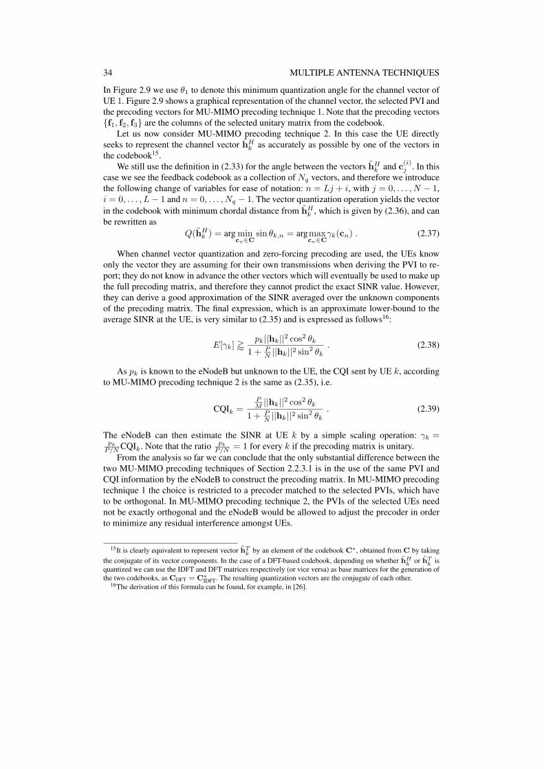
34 MULTIPLE ANTENNA TECHNIQUES
In Figure 2.9 we use θ1 to denote this minimum quantization angle for the channel vector ofUE 1. Figure 2.9 shows a graphical representation of the channel vector, the selected PVI andthe precoding vectors for MU-MIMO precoding technique 1. Note that the precoding vectors{f1, f2, f3} are the columns of the selected unitary matrix from the codebook.
Let us now consider MU-MIMO precoding technique 2. In this case the UE directlyseeks to represent the channel vector hH
k as accurately as possible by one of the vectors inthe codebook15.
We still use the definition in (2.33) for the angle between the vectors hHk and c(i)
j . In thiscase we see the feedback codebook as a collection of Nq vectors, and therefore we introducethe following change of variables for ease of notation: n = Lj + i, with j = 0, . . . , N − 1,i = 0, . . . , L− 1 and n = 0, . . . , Nq − 1. The vector quantization operation yields the vectorin the codebook with minimum chordal distance from hH
k , which is given by (2.36), and canbe rewritten as
Q(hHk ) = arg min
cn∈Csin θk,n = argmax
cn∈Cγk(cn) . (2.37)
When channel vector quantization and zero-forcing precoding are used, the UEs knowonly the vector they are assuming for their own transmissions when deriving the PVI to re-port; they do not know in advance the other vectors which will eventually be used to make upthe full precoding matrix, and therefore they cannot predict the exact SINR value. However,they can derive a good approximation of the SINR averaged over the unknown componentsof the precoding matrix. The final expression, which is an approximate lower-bound to theaverage SINR at the UE, is very similar to (2.35) and is expressed as follows16:
E[γk] 'pk||hk||2 cos2 θk
1 + PN ||hk||2 sin2 θk
. (2.38)
As pk is known to the eNodeB but unknown to the UE, the CQI sent by UE k, accordingto MU-MIMO precoding technique 2 is the same as (2.35), i.e.
CQIk =PM ||hk||2 cos2 θk
1 + PN ||hk||2 sin2 θk
. (2.39)
The eNodeB can then estimate the SINR at UE k by a simple scaling operation: γk =pk
P/N CQIk. Note that the ratio pk
P/N = 1 for every k if the precoding matrix is unitary.From the analysis so far we can conclude that the only substantial difference between the
two MU-MIMO precoding techniques of Section 2.2.3.1 is in the use of the same PVI andCQI information by the eNodeB to construct the precoding matrix. In MU-MIMO precodingtechnique 1 the choice is restricted to a precoder matched to the selected PVIs, which haveto be orthogonal. In MU-MIMO precoding technique 2, the PVIs of the selected UEs neednot be exactly orthogonal and the eNodeB would be allowed to adjust the precoder in orderto minimize any residual interference amongst UEs.
15It is clearly equivalent to represent vector hTk by an element of the codebook C∗, obtained from C by taking
the conjugate of its vector components. In the case of a DFT-based codebook, depending on whether hHk or hT
k isquantized we can use the IDFT and DFT matrices respectively (or vice versa) as base matrices for the generation ofthe two codebooks, as CDFT = C∗
IDFT. The resulting quantization vectors are the conjugate of each other.16The derivation of this formula can be found, for example, in [26].

MULTIPLE ANTENNA TECHNIQUES 35
In practice, only unitary codebooks are provided in the first version of LTE, and PDSCHtransmission in MU-MIMO mode17 is based on selection of precoding matrices from thesame codebooks as are used for SU-MIMO (as summarized in Section 2.2.2.3 above).
In the light of the above discussion on MU-MIMO techniques, it is instructive to observethat the LTE 2-antenna codebook, and also the first 8 entries in the 4-antenna codebook, are infact DFT-based codebooks — in other words derived from a discrete Fourier transformationmatrix. The main reasons for this choice are as follows:
a. Simplicity in the PVI/CQI calculation, which can be done in some cases without com-plex multiplications;
b. The fact that a DFT matrix nicely captures the characteristics of a highly correlatedMISO channel. In fact, it is not difficult to see that, if the first N rows are taken froma DFT matrix of size Nq, each of the Nq column vectors that is obtained contains thephases of (i.e. the baseband representation of) a line-of-sight propagation channel froma uniform linear array with N elements to a point in space located at a given angle withrespect to the antenna array boresight (see for example [24]).
c. It is also easy to verify that the vectors in such a codebook can be grouped into L =Nq/N unitary matrices.
2.2.3.3 User selection mechanism
As is clear from the discussion above, one important aspect of MU-MIMO precoding is theselection of UEs for transmission, as the throughput gain of na ïve linear precoding tech-niques very much depends on exploiting the multi-user diversity available in the system.Although the method for selecting UEs is not specified in LTE or other similar systems, webriefly review two very simple strategies which could be appropriate for implementation inconjunction with the precoding methods we have considered.
One simple way of selecting UEs, according to MU-MIMO precoding technique 1 ofSection 2.2.3.1, is to group UEs that report orthogonal PVIs and select the group providingthe highest total throughput. This can be simply estimated, for example from the capacityformula R =
∑k (1 + log SINRk), where the summation is over the UEs in the group and
the SINR value is given by the CQI.Another more general and very simple greedy strategy, which would be appropriate for
MU-MIMO precoding technique 2, consists of adding one UE at a time, as long as the ad-ditional UE increases the overall throughput, estimated according to a criterion such as theachievable sum-rate. This simple strategy can be described as follows (see, for example [7]).Let R(S) denote the achievable sum-rate when the set of UEs S is selected for transmission.
Algorithm 1 User SelectionInitialize S = ∅, R(S) = 0.while|S| ≤ N do
1. k = argmaxk/∈S
R(S ∪ {k})
2. if R(S ∪ {k}) > R(S) update S = S ∪ {k}, else exit.
17PDSCH transmission mode 5 — see Section ??

36 MULTIPLE ANTENNA TECHNIQUES
2.2.3.4 Receiver spatial equalizers
Since in LTE each UE is assumed to support two receiving antennas, it is important to con-sider the possible receive beamforming structures for MU-MIMO transmission, which mayaffect the PVI and CQI calculation.18
We consider the possibilities for receiver beamforming in terms of a generic UE k withJ antenna elements, and we use Hk = [hT
1 , . . . ,hTJ ]T to denote a J ×N channel for that
UE. We also use Hk = HkF = [hk,0, . . . , hk,N−1] to denote the product matrix betweenthe reference UE’s channel and the precoder, as defined in (2.29).
Using this terminology, we describe three possible spatial equalizers, which all attemptto maximize the received SINR, with different degrees of knowledge at the UE side:
1. MMSE receiver. If the precoding vector for the reference UE k corresponds to the jth
column of F, then the 1× J vector of receiver combining coefficients, wk,j , is givenby19
wk,j = hHk,j
(HkHH
k + IJ
)−1. (2.40)
This receiver requires that the user estimate the N vectors of size J in the productmatrix Hk. This knowledge can be acquired by estimating the channel matrix fromthe common RS and being told by explicit signalling which precoding matrix is used.Alternatively, if precoded RS were to be provided, the product matrix could be directlyestimated from them. It goes without saying that the former method is best suited fora MU-MIMO scheme with a small set of possible precoding matrices, whilst the latterallows for full flexibility in the construction of the precoding matrix.
2. Minimum quantization error (MQE) receiver. In this case, for a given vector of thecodebook, cn, the coefficients of the linear combination at the receiver k are given by
wk,n = αh(eff)k,n H†
k , (2.41)
where H†k = HH
k (HkHHk )−1 is the right pseudo-inverse of Hk, α is a normaliza-
tion factor, such that ‖wk,n‖ = 1, and (the row vector) h(eff)k,n is the projection of cH
n
onto span(HTk ). To express this algebraically, let QT
k = [qTk,1, . . . ,q
Tk,J ] be a generator
matrix for span(HTk ), then
h(eff)k,n = cH
n QHk Qk . (2.42)
For the derivation of this receiver we refer the interested reader to [15]. Note that thestructure of (2.41) is very similar to (2.40), but calculation of (2.41) does not requireknowledge of the precoding matrix. This is because it minimizes the vector quantiza-tion error independently of the transmit beamformer, and by so doing it also maximizesthe CQI value (2.39).
3. SVD of the channel. This na ve receive beamformer depends only on the channelmatrix Hk and is independent of any CSI feedback. Let Hk = UkΛkTH
k be the SVD
18Note that receiver algorithms are not defined in the specifications; instead, the required demodulation perfor-mance is specified.
19Note that the noise variance is normalized to 1 as it is included in the transmit SNR, P .

MULTIPLE ANTENNA TECHNIQUES 37
of the channel, with singular values λk,1 ≥ λk,2 ≥ · · · ≥ λk,J (J ≤ N ), and Uk =[uk,1, . . . ,uk,J ]. Then
wk = uHk,1 . (2.43)
2.2.4 Physical-layer MIMO performanceIn this section we present some link-level and system-level simulation results to illustratethe physical layer performance of various MIMO schemes, starting with single-user MIMOand then followed by multi-user MIMO schemes. Some of these results were influential indeciding on the MIMO schemes for LTE.
2.2.4.1 Precoding Performance
To demonstrate the benefits of precoding, link-level simulation results [13] in Figures 2.11and 2.12 show the percentage throughput gains versus geometry (average SINR) when com-pared to antenna selection. The channel model here is the SCM-D (see Section ??) witha uniform linear array with 4λ (uncorrelated frequency selective fading) antenna spacing.Clearly the precoding gains are greater in the 4× 2 case than in the 4× 4 case, as expected.Similar gains compared to antenna selection are shown in [23]. The legends in Figures referto different codebook designs as follows:
• CMHH : Constant Modulus Householder
• 4-DFT: Codebook based on Four DFT matrices. This is also referred to as the unop-timized or regular DFT codebook, since the different matrices are not optimized tomaximize the minimum chordal distance.
The 4-antenna LTE codebook has similar performance to the CMHH codebook.
2.2.4.2 Multi-user MIMO performance
We here consider the two MU-MIMO precoding techniques discussed in Section 2.2.3.1,namely unitary precoding and zero-forcing precoding with equal power distribution acrossthe selected UEs. We consider the case with N = 4 transmit antennas at the eNodeB andM = 1, 2 receive antennas per UE.
The main parameters used for the link-level simulations are listed in Table 2.3.In Figure 2.13 the throughput is plotted versus average SNR for unitary precoding and
zero-forcing precoding. As the codebook size increases, unitary precoding shows degrada-tion due to the scheduling problem discussed earlier, namely that too few UEs select the sameprecoding matrix, thus making full-rank transmission less likely. As a consequence, the mul-tiplexing gain for large codebooks falls to one, as for TDMA. The gap between the TDMAcurve and the unitary precoding curves for large codebook sizes is due to the fact that forTDMA we assume that the eNodeB always matches the transmit beamformer to the reportedchannel vector. It is possible to devise various techniques to mitigate the scheduling problemof unitary precoding, for example by overruling the UE’s selected matrix according to somecriterion.
For a large number of UEs available for transmission, unitary precoding and zero-forcingwill perform the same, as it becomes increasingly likely that a set of N UEs can be found with

38 MULTIPLE ANTENNA TECHNIQUES
−5 0 5 10 15 200
2
4
6
8
10
12
14
16
18
20
Geometry (dB)
% T
hro
ug
hp
ut
Ga
ins o
ve
r V
irtu
al A
S
4x2 , ULA 4L, SCME−D
4−DFT
CMHH
Figure 2.11 Throughput gain achieved by precoding with two different codebooks, comparedto antenna selection: 4× 2.
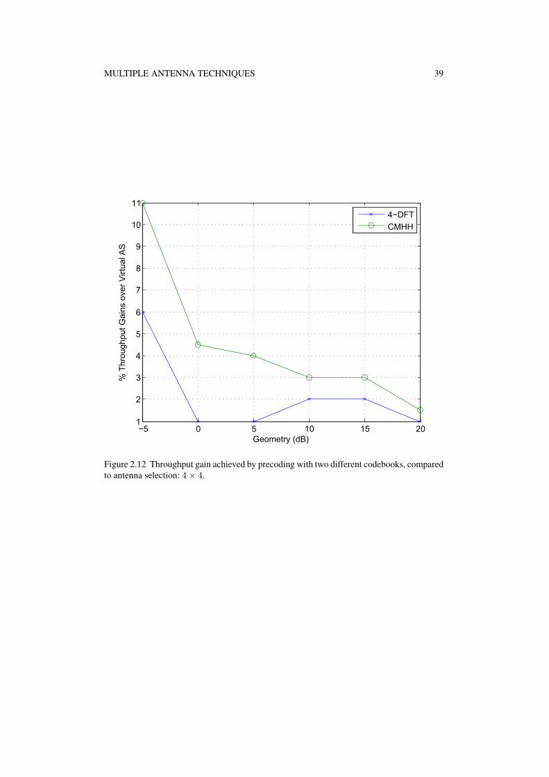
MULTIPLE ANTENNA TECHNIQUES 39
−5 0 5 10 15 201
2
3
4
5
6
7
8
9
10
114x4, ULA 4L, SCME−D
Geometry (dB)
% T
hro
ug
hp
ut
Ga
ins o
ve
r V
irtu
al A
S
4−DFT
CMHH
Figure 2.12 Throughput gain achieved by precoding with two different codebooks, comparedto antenna selection: 4× 4.
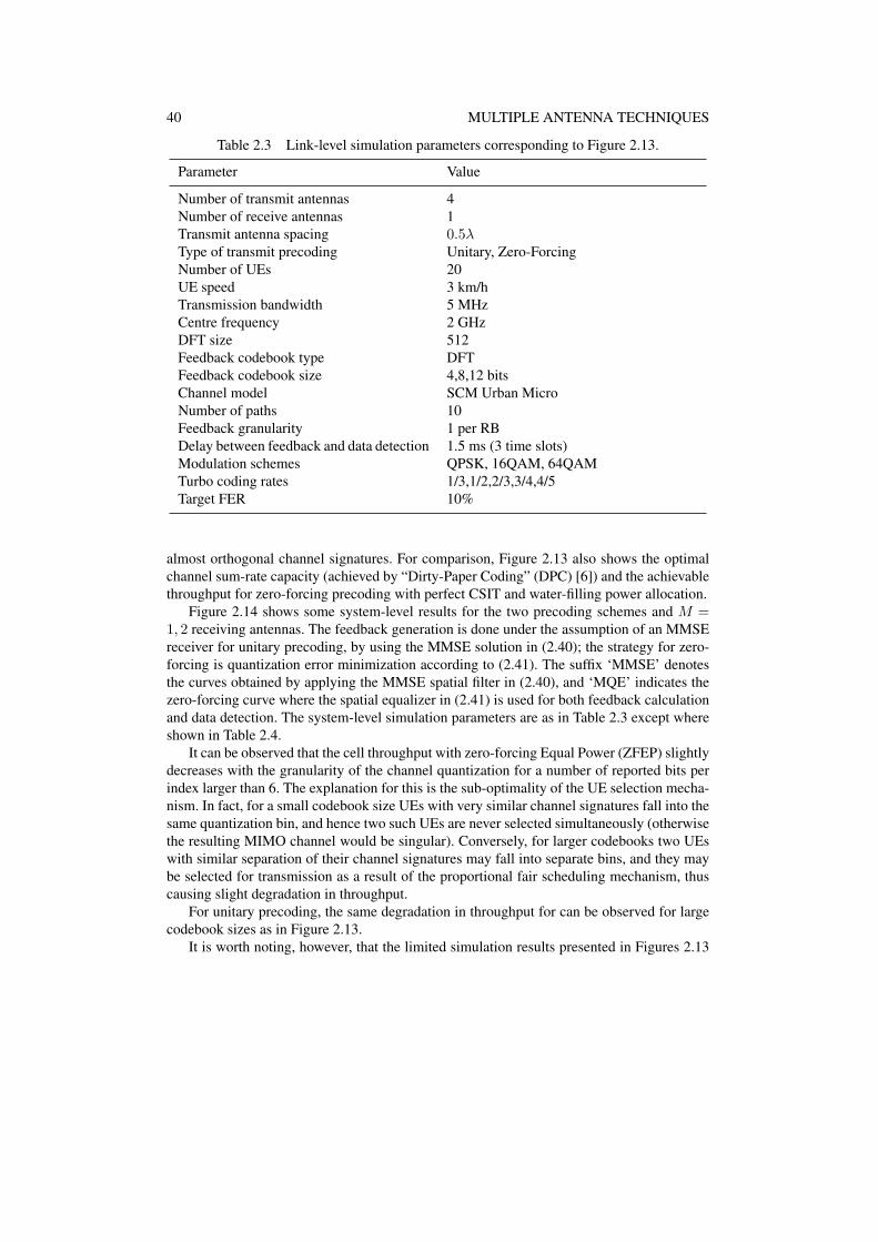
40 MULTIPLE ANTENNA TECHNIQUES
Table 2.3 Link-level simulation parameters corresponding to Figure 2.13.
Parameter Value
Number of transmit antennas 4Number of receive antennas 1Transmit antenna spacing 0.5λType of transmit precoding Unitary, Zero-ForcingNumber of UEs 20UE speed 3 km/hTransmission bandwidth 5 MHzCentre frequency 2 GHzDFT size 512Feedback codebook type DFTFeedback codebook size 4,8,12 bitsChannel model SCM Urban MicroNumber of paths 10Feedback granularity 1 per RBDelay between feedback and data detection 1.5 ms (3 time slots)Modulation schemes QPSK, 16QAM, 64QAMTurbo coding rates 1/3,1/2,2/3,3/4,4/5Target FER 10%
almost orthogonal channel signatures. For comparison, Figure 2.13 also shows the optimalchannel sum-rate capacity (achieved by “Dirty-Paper Coding” (DPC) [6]) and the achievablethroughput for zero-forcing precoding with perfect CSIT and water-filling power allocation.
Figure 2.14 shows some system-level results for the two precoding schemes and M =1, 2 receiving antennas. The feedback generation is done under the assumption of an MMSEreceiver for unitary precoding, by using the MMSE solution in (2.40); the strategy for zero-forcing is quantization error minimization according to (2.41). The suffix ‘MMSE’ denotesthe curves obtained by applying the MMSE spatial filter in (2.40), and ‘MQE’ indicates thezero-forcing curve where the spatial equalizer in (2.41) is used for both feedback calculationand data detection. The system-level simulation parameters are as in Table 2.3 except whereshown in Table 2.4.
It can be observed that the cell throughput with zero-forcing Equal Power (ZFEP) slightlydecreases with the granularity of the channel quantization for a number of reported bits perindex larger than 6. The explanation for this is the sub-optimality of the UE selection mecha-nism. In fact, for a small codebook size UEs with very similar channel signatures fall into thesame quantization bin, and hence two such UEs are never selected simultaneously (otherwisethe resulting MIMO channel would be singular). Conversely, for larger codebooks two UEswith similar separation of their channel signatures may fall into separate bins, and they maybe selected for transmission as a result of the proportional fair scheduling mechanism, thuscausing slight degradation in throughput.
For unitary precoding, the same degradation in throughput for can be observed for largecodebook sizes as in Figure 2.13.
It is worth noting, however, that the limited simulation results presented in Figures 2.13
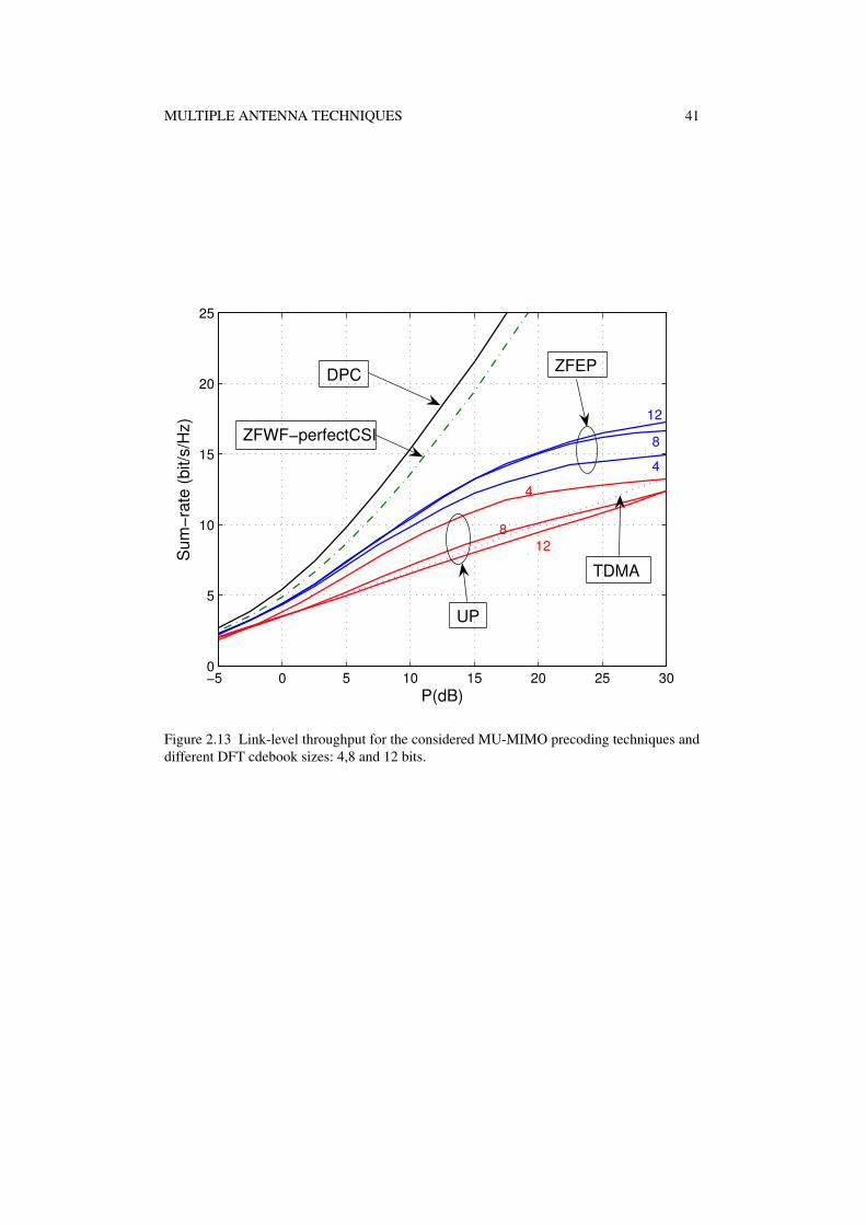
MULTIPLE ANTENNA TECHNIQUES 41
−5 0 5 10 15 20 25 300
5
10
15
20
25
P(dB)
Su
m−
rate
(b
it/s
/Hz)
N=4,M=1,U=20,SCM−Urban Micro 10Paths,B=4,8,12
DPC
ZFWF−perfectCSI
4
8
12
4
8
12
ZFEP
UP
TDMA
Figure 2.13 Link-level throughput for the considered MU-MIMO precoding techniques anddifferent DFT cdebook sizes: 4,8 and 12 bits.
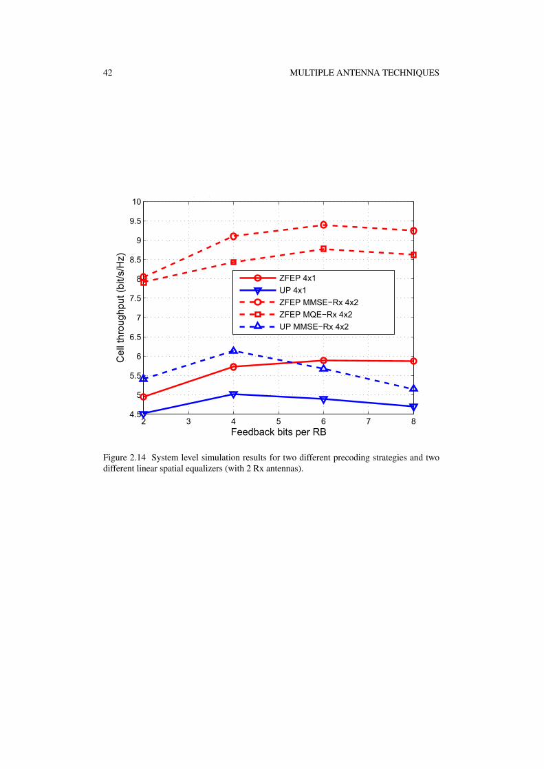
42 MULTIPLE ANTENNA TECHNIQUES
2 3 4 5 6 7 84.5
5
5.5
6
6.5
7
7.5
8
8.5
9
9.5
10
Feedback bits per RB
Ce
ll th
rou
gh
pu
t (b
it/s
/Hz)
N=4, M={1,2}, U=20 per cell, SCM−Urban micro 10 paths
ZFEP 4x1
UP 4x1
ZFEP MMSE−Rx 4x2
ZFEP MQE−Rx 4x2
UP MMSE−Rx 4x2
Figure 2.14 System level simulation results for two different precoding strategies and twodifferent linear spatial equalizers (with 2 Rx antennas).

MULTIPLE ANTENNA TECHNIQUES 43
Table 2.4 System-level simulation parameters corresponding to Figure 2.14.
Parameter Value
Number of receive antennas 1,2Transmit antenna spacing 10λReceive antenna spacing 0.5λType of rx beamforming MMSE, min. quant. error (MQE)Cellular layout hexagonal grid, 19 cell sites, 3 sectors per
siteInter-site distance 2 KmThermal noise spectral density -174 dBm/HzShadowing lognormal (8 dB)Transmit power 20 WFront-to-back ratio of eNodeB antennas 20 dBPath loss exponent 4Frequency re-use factor 1Feedback codebook size 2-8 bitsTraffic model full queue trafficScheduling algorithm proportional fair schedulingProportional fair factor 1Hybrid ARQ Chase combiningMax. number of retransmissions 4
and 2.14 do not show the performance degradation of zero-forcing beamforming compared tounitary precoding which may occur if the reported channel feedback information is very in-accurate. In general, zero-forcing beamforming can be less robust against inaccuracies in thechannel representation compared to unitary precoding. This would be the case, for example,if the feedback were to be reported with a coarser frequency granularity than the coherencebandwidth of the channel, or if the codebook size for the channel feedback is small. A similarsituation occurs when the channels are spatially highly uncorrelated: in such a case the “direc-tion” of a channel signature may change significantly between groups of adjacent sub-carriersand it becomes harder to provide an accurate channel representation consistently across fre-quency, compared to the case of spatially correlated channels. In such cases, where it is notpossible to provide sufficiently accurate channel information to the transmitter, the unitaryprecoding adopted in the first version of LTE can prove more robust and than a zero-forcingapproach.
2.2.5 Concluding RemarksWe have reviewed the predominant families of MU-MIMO techniques of relevance to thefirst and future versions of LTE. LTE breaks new ground in drawing on such approaches toharness the power of MIMO systems not just for boosting the peak per-user data rate but alsofor improving overall system capacity and spectral efficiency. It is clear, however, that theearly techniques leave substantial scope for further development and enhancement in laterreleases of the LTE specifications.


Bibliography
[1] 3GPP Technical Specification 36.211, "E-UTRA physical channels and modulation (Release 8)"www.3gpp.org.
[2] S. M. Alamouti, “A Simple Transmitter Diversity Technique for Wireless Communications”.IEEE Journal on Selected Areas in Communications, Vol. 16, pp. 1451–1458, October 1998.
[3] H. Bölcskei, D. Gesbert, C. Papadias, and A. J. van der Veen (Eds.), Space-Time Wireless Systems:From Array Processing to MIMO Communications. Cambridge Univ. Press, 2006.
[4] Caire, G. and Shamai, S. (Shitz), “On the achievable throughput of a multi-antenna Gaussianbroadcast channel". IEEE Trans. Info. Th., Vol. 49, pp. 1691–1706, July 2003.
[5] J.H. Conway, R.H. Hardin, and N.J.A. Sloane, "Packing lines, planes, etc.: packings in Grassman-nian frames" AT&T Bell Laboratories, Apr. 1996, Unpublished report available online.
[6] M. Costa, “Writing on dirty paper”. IEEE Trans. on Information Theory, Vol. 29, pp. 439–441,May 1983.
[7] G. Dimic and N. Sidiropoulos, “On downlink beamforming with greedy user selection: per-formance analysis and simple new algorithm". IEEE Trans. on Signal Processing, Vol. 53,pp. 3857–3868, October 2005.
[8] P. Ding, D. J. Love, and M. D. Zoltowski, “Multiple antenna broadcast channels with shapefeedback and limited feedback". IEEE Trans. on Signal Processing, Vol. 55, pp. 3417–3428, July2007.
[9] D. Gesbert, M. Shafi, P. Smith, D. Shiu, and A. Naguib, “From theory to practice: An overview ofMIMO space-time coded wireless systems". IEEE Journal on Selected Areas in Communications.Special Issue on MIMO systems, guest edited by the authors, April 2003.
[10] A. Goldsmith, Wireless Communications. Cambridge University Press, 2005.
[11] G. Golub and C. van Loan, “Matrix Computations”. John Hopkins University Press, 1996.
[12] Heath, R. and Lau, V. and Love, D. and Gesbert, D. and Rao, B. and Andrews, A. (Eds.), Exploit-ing limited feedback in tomorrow’s wireless communications networks. Special issue of IEEEJournal on Selected Areas in Communications, October 2008.
[13] Texas Instruments, “R1-072844: Link Level Evaluation of 4-TX Codebook for SU-MIMO" June2007.
[14] N. Jindal, “MIMO broadcast channels with finite rate feedback" in in Proc. GLOBECOM’05,pp. 1520–1524, 2005.
[15] N. Jindal, “A feedback reduction technique for MIMO broadcast channels" in IEEE Int. Symp. onInform. Theory, pp. 2699–2703, July 2006.
[16] N. Jindal, “MIMO Broadcast Channels with Finite Rate Feedback". IEEE Trans. Info. Th.,Vol. 52, pp. 5045–5059, November 2006.
46 BIBLIOGRAPHY
[17] F. Kaltenberger, L. S. Cardoso, M. Kountouris, R. Knopp, and D. Gesbert, “Capacity of linearmulti-user MIMO precoding schemes with measured channel data" in Proc. IEEE Intl. Work-shop on Signal Processing Advances in Wireless Communications (SPAWC), (Recife, Brazil), July2008.
[18] F. Kaltenberger, M. Kountouris, D. Gesbert, and R. Knopp, “Correlation and Capacity of Mea-sured Multi-user MIMO Channels" in Proc. IEEE Intl. Symposium on Personal, Indoor andMobile Radio Communications (PIMRC), (Cannes, France), September 2008.
[19] D. Love, R. Heath Jr., and T. Strohmer, “Grassmannian beamforming for multiple-input multiple-output wireless systems". IEEE Trans. on Information Theory, Vol. 49, pp. 2735–2747, October2003.
[20] Love, D. and Heath Jr., R. and Santipach, W. and Honig, M. , “What is the Value of LimitedFeedback for MIMO Channels?”. IEEE Comm. Mag., Vol. 42, pp. 54–59, October 2003.
[21] A. Narula, M. J. Lopez, M. D. Trott, and G. W. Wornell, “Efficient use of side information inmultiple antenna data transmission over fading channels". IEEE Journal on Selected Areas inCommunications, Vol. 16, pp. 1223–1436, October 1998.
[22] A. Osseiran and A. Logothetis, “Closed loop transmit diversity in WCDMA HS-DSCH” in IEEEVTC Spring, May 2005.
[23] Samsung, “R1-073181:Way-forward on Codebook for SU-MIMO Precoding" June 2007.[24] D. Tse and P. Viswanath, Fundamentals of Wireless Communication. Cambridge University Press,
2004.[25] T. Yoo and A. Goldsmith, “On the optimality of multiantenna broadcast scheduling using zero-
forcing beamforming". IEEE Journal on Selected Areas in Communications, Vol. 24, pp. 528–541,March 2006.
[26] T. Yoo, N. Jindal, and A. Goldsmith, “Multi-antenna downlink channels with limited feedbackand user selection". IEEE Journal on Selected Areas in Communications, Vol. 25, pp. 1478–1491,September 2007.
[27] R. Zakhour and D. Gesbert, Adaptive Feedback Rate Control in MIMO Broadcast Systems in Proc.of the IEEE Information Theory Workshop, (San Diego, Ca., USA), Jan. 2008.
Bibliography
[1] 3GPP Technical Specification 36.211, "E-UTRA physical channels and modulation (Release 8)"www.3gpp.org.
[2] S. M. Alamouti, “A Simple Transmitter Diversity Technique for Wireless Communications”.IEEE Journal on Selected Areas in Communications, Vol. 16, pp. 1451–1458, October 1998.
[3] H. Bölcskei, D. Gesbert, C. Papadias, and A. J. van der Veen (Eds.), Space-Time Wireless Systems:From Array Processing to MIMO Communications. Cambridge Univ. Press, 2006.
[4] Caire, G. and Shamai, S. (Shitz), “On the achievable throughput of a multi-antenna Gaussianbroadcast channel". IEEE Trans. Info. Th., Vol. 49, pp. 1691–1706, July 2003.
[5] J.H. Conway, R.H. Hardin, and N.J.A. Sloane, "Packing lines, planes, etc.: packings in Grassman-nian frames" AT&T Bell Laboratories, Apr. 1996, Unpublished report available online.
[6] M. Costa, “Writing on dirty paper”. IEEE Trans. on Information Theory, Vol. 29, pp. 439–441,May 1983.
[7] G. Dimic and N. Sidiropoulos, “On downlink beamforming with greedy user selection: per-formance analysis and simple new algorithm". IEEE Trans. on Signal Processing, Vol. 53,pp. 3857–3868, October 2005.
[8] P. Ding, D. J. Love, and M. D. Zoltowski, “Multiple antenna broadcast channels with shapefeedback and limited feedback". IEEE Trans. on Signal Processing, Vol. 55, pp. 3417–3428, July2007.
[9] D. Gesbert, M. Shafi, P. Smith, D. Shiu, and A. Naguib, “From theory to practice: An overview ofMIMO space-time coded wireless systems". IEEE Journal on Selected Areas in Communications.Special Issue on MIMO systems, guest edited by the authors, April 2003.
[10] A. Goldsmith, Wireless Communications. Cambridge University Press, 2005.
[11] G. Golub and C. van Loan, “Matrix Computations”. John Hopkins University Press, 1996.
[12] Heath, R. and Lau, V. and Love, D. and Gesbert, D. and Rao, B. and Andrews, A. (Eds.), Exploit-ing limited feedback in tomorrow’s wireless communications networks. Special issue of IEEEJournal on Selected Areas in Communications, October 2008.
[13] Texas Instruments, “R1-072844: Link Level Evaluation of 4-TX Codebook for SU-MIMO" June2007.
[14] N. Jindal, “MIMO broadcast channels with finite rate feedback" in in Proc. GLOBECOM’05,pp. 1520–1524, 2005.
[15] N. Jindal, “A feedback reduction technique for MIMO broadcast channels" in IEEE Int. Symp. onInform. Theory, pp. 2699–2703, July 2006.
[16] N. Jindal, “MIMO Broadcast Channels with Finite Rate Feedback". IEEE Trans. Info. Th.,Vol. 52, pp. 5045–5059, November 2006.

48 BIBLIOGRAPHY
[17] F. Kaltenberger, L. S. Cardoso, M. Kountouris, R. Knopp, and D. Gesbert, “Capacity of linearmulti-user MIMO precoding schemes with measured channel data" in Proc. IEEE Intl. Work-shop on Signal Processing Advances in Wireless Communications (SPAWC), (Recife, Brazil), July2008.
[18] F. Kaltenberger, M. Kountouris, D. Gesbert, and R. Knopp, “Correlation and Capacity of Mea-sured Multi-user MIMO Channels" in Proc. IEEE Intl. Symposium on Personal, Indoor andMobile Radio Communications (PIMRC), (Cannes, France), September 2008.
[19] D. Love, R. Heath Jr., and T. Strohmer, “Grassmannian beamforming for multiple-input multiple-output wireless systems". IEEE Trans. on Information Theory, Vol. 49, pp. 2735–2747, October2003.
[20] Love, D. and Heath Jr., R. and Santipach, W. and Honig, M. , “What is the Value of LimitedFeedback for MIMO Channels?”. IEEE Comm. Mag., Vol. 42, pp. 54–59, October 2003.
[21] A. Narula, M. J. Lopez, M. D. Trott, and G. W. Wornell, “Efficient use of side information inmultiple antenna data transmission over fading channels". IEEE Journal on Selected Areas inCommunications, Vol. 16, pp. 1223–1436, October 1998.
[22] A. Osseiran and A. Logothetis, “Closed loop transmit diversity in WCDMA HS-DSCH” in IEEEVTC Spring, May 2005.
[23] Samsung, “R1-073181:Way-forward on Codebook for SU-MIMO Precoding" June 2007.[24] D. Tse and P. Viswanath, Fundamentals of Wireless Communication. Cambridge University Press,
2004.[25] T. Yoo and A. Goldsmith, “On the optimality of multiantenna broadcast scheduling using zero-
forcing beamforming". IEEE Journal on Selected Areas in Communications, Vol. 24, pp. 528–541,March 2006.
[26] T. Yoo, N. Jindal, and A. Goldsmith, “Multi-antenna downlink channels with limited feedbackand user selection". IEEE Journal on Selected Areas in Communications, Vol. 25, pp. 1478–1491,September 2007.
[27] R. Zakhour and D. Gesbert, Adaptive Feedback Rate Control in MIMO Broadcast Systems in Proc.of the IEEE Information Theory Workshop, (San Diego, Ca., USA), Jan. 2008.