getting start mathlab 2010
TRANSCRIPT
MATLAB® 7Getting Started Guide
How to Contact MathWorks
www.mathworks.com Webcomp.soft-sys.matlab Newsgroupwww.mathworks.com/contact_TS.html Technical Support
[email protected] Product enhancement [email protected] Bug [email protected] Documentation error [email protected] Order status, license renewals, [email protected] Sales, pricing, and general information
508-647-7000 (Phone)
508-647-7001 (Fax)
The MathWorks, Inc.3 Apple Hill DriveNatick, MA 01760-2098For contact information about worldwide offices, see the MathWorks Web site.
MATLAB® Getting Started Guide
© COPYRIGHT 1984–2011 by The MathWorks, Inc.The software described in this document is furnished under a license agreement. The software may be usedor copied only under the terms of the license agreement. No part of this manual may be photocopied orreproduced in any form without prior written consent from The MathWorks, Inc.
FEDERAL ACQUISITION: This provision applies to all acquisitions of the Program and Documentationby, for, or through the federal government of the United States. By accepting delivery of the Programor Documentation, the government hereby agrees that this software or documentation qualifies ascommercial computer software or commercial computer software documentation as such terms are usedor defined in FAR 12.212, DFARS Part 227.72, and DFARS 252.227-7014. Accordingly, the terms andconditions of this Agreement and only those rights specified in this Agreement, shall pertain to and governthe use, modification, reproduction, release, performance, display, and disclosure of the Program andDocumentation by the federal government (or other entity acquiring for or through the federal government)and shall supersede any conflicting contractual terms or conditions. If this License fails to meet thegovernment’s needs or is inconsistent in any respect with federal procurement law, the government agreesto return the Program and Documentation, unused, to The MathWorks, Inc.
Trademarks
MATLAB and Simulink are registered trademarks of The MathWorks, Inc. Seewww.mathworks.com/trademarks for a list of additional trademarks. Other product or brandnames may be trademarks or registered trademarks of their respective holders.
Patents
MathWorks products are protected by one or more U.S. patents. Please seewww.mathworks.com/patents for more information.
Revision HistoryDecember 1996 First printing For MATLAB 5May 1997 Second printing For MATLAB 5.1September 1998 Third printing For MATLAB 5.3September 2000 Fourth printing Revised for MATLAB 6 (Release 12)June 2001 Online only Revised for MATLAB 6.1 (Release 12.1)July 2002 Online only Revised for MATLAB 6.5 (Release 13)August 2002 Fifth printing Revised for MATLAB 6.5June 2004 Sixth printing Revised for MATLAB 7.0 (Release 14)October 2004 Online only Revised for MATLAB 7.0.1 (Release 14SP1)March 2005 Online only Revised for MATLAB 7.0.4 (Release 14SP2)June 2005 Seventh printing Minor revision for MATLAB 7.0.4 (Release 14SP2)September 2005 Online only Minor revision for MATLAB 7.1 (Release 14SP3)March 2006 Online only Minor revision for MATLAB 7.2 (Release 2006a)September 2006 Eighth printing Minor revision for MATLAB 7.3 (Release 2006b)March 2007 Ninth printing Minor revision for MATLAB 7.4 (Release 2007a)September 2007 Tenth printing Minor revision for MATLAB 7.5 (Release 2007b)March 2008 Eleventh printing Minor revision for MATLAB 7.6 (Release 2008a)October 2008 Twelfth printing Minor revision for MATLAB 7.7 (Release 2008b)March 2009 Thirteenth printing Minor revision for MATLAB 7.8 (Release 2009a)September 2009 Fourteenth printing Minor revision for MATLAB 7.9 (Release 2009b)March 2010 Fifteenth printing Minor revision for MATLAB 7.10 (Release 2010a)September 2010 Sixteenth printing Revised for MATLAB 7.11 (R2010b)April 2011 Online only Revised for MATLAB 7.12 (R2011a)

Contents
Getting Started
Introduction
1Product Overview . . . . . . . . . . . . . . . . . . . . . . . . . . . . . . . . . 1-2Overview of the MATLAB Environment . . . . . . . . . . . . . . . 1-2The MATLAB System . . . . . . . . . . . . . . . . . . . . . . . . . . . . . . 1-3
Documentation . . . . . . . . . . . . . . . . . . . . . . . . . . . . . . . . . . . . 1-5
Starting and Quitting the MATLAB Program . . . . . . . . . 1-7Starting a MATLAB Session . . . . . . . . . . . . . . . . . . . . . . . . 1-7Quitting the MATLAB Program . . . . . . . . . . . . . . . . . . . . . . 1-8
Matrices and Arrays
2Matrices and Magic Squares . . . . . . . . . . . . . . . . . . . . . . . . 2-2About Matrices . . . . . . . . . . . . . . . . . . . . . . . . . . . . . . . . . . . 2-2Entering Matrices . . . . . . . . . . . . . . . . . . . . . . . . . . . . . . . . . 2-4sum, transpose, and diag . . . . . . . . . . . . . . . . . . . . . . . . . . . 2-5Subscripts . . . . . . . . . . . . . . . . . . . . . . . . . . . . . . . . . . . . . . . 2-7The Colon Operator . . . . . . . . . . . . . . . . . . . . . . . . . . . . . . . . 2-8The magic Function . . . . . . . . . . . . . . . . . . . . . . . . . . . . . . . . 2-9
Expressions . . . . . . . . . . . . . . . . . . . . . . . . . . . . . . . . . . . . . . . 2-11Variables . . . . . . . . . . . . . . . . . . . . . . . . . . . . . . . . . . . . . . . . 2-11Numbers . . . . . . . . . . . . . . . . . . . . . . . . . . . . . . . . . . . . . . . . 2-12Operators . . . . . . . . . . . . . . . . . . . . . . . . . . . . . . . . . . . . . . . . 2-13
v
Functions . . . . . . . . . . . . . . . . . . . . . . . . . . . . . . . . . . . . . . . . 2-14Examples of Expressions . . . . . . . . . . . . . . . . . . . . . . . . . . . 2-15
Working with Matrices . . . . . . . . . . . . . . . . . . . . . . . . . . . . . 2-17Generating Matrices . . . . . . . . . . . . . . . . . . . . . . . . . . . . . . . 2-17The load Function . . . . . . . . . . . . . . . . . . . . . . . . . . . . . . . . . 2-18Saving Code to a File . . . . . . . . . . . . . . . . . . . . . . . . . . . . . . 2-18Concatenation . . . . . . . . . . . . . . . . . . . . . . . . . . . . . . . . . . . . 2-19Deleting Rows and Columns . . . . . . . . . . . . . . . . . . . . . . . . . 2-20
More About Matrices and Arrays . . . . . . . . . . . . . . . . . . . . 2-21Linear Algebra . . . . . . . . . . . . . . . . . . . . . . . . . . . . . . . . . . . . 2-21Arrays . . . . . . . . . . . . . . . . . . . . . . . . . . . . . . . . . . . . . . . . . . 2-25Multivariate Data . . . . . . . . . . . . . . . . . . . . . . . . . . . . . . . . . 2-27Scalar Expansion . . . . . . . . . . . . . . . . . . . . . . . . . . . . . . . . . . 2-28Logical Subscripting . . . . . . . . . . . . . . . . . . . . . . . . . . . . . . . 2-28The find Function . . . . . . . . . . . . . . . . . . . . . . . . . . . . . . . . . 2-29
Controlling Command Window Input and Output . . . . 2-31The format Function . . . . . . . . . . . . . . . . . . . . . . . . . . . . . . . 2-31Suppressing Output . . . . . . . . . . . . . . . . . . . . . . . . . . . . . . . 2-32Entering Long Statements . . . . . . . . . . . . . . . . . . . . . . . . . . 2-33Command Line Editing . . . . . . . . . . . . . . . . . . . . . . . . . . . . . 2-33
Graphics
3Overview of Plotting . . . . . . . . . . . . . . . . . . . . . . . . . . . . . . . 3-2Plotting Process . . . . . . . . . . . . . . . . . . . . . . . . . . . . . . . . . . . 3-2Graph Components . . . . . . . . . . . . . . . . . . . . . . . . . . . . . . . . 3-6Figure Tools . . . . . . . . . . . . . . . . . . . . . . . . . . . . . . . . . . . . . . 3-7Arranging Graphs Within a Figure . . . . . . . . . . . . . . . . . . . 3-14Choosing a Type of Graph to Plot . . . . . . . . . . . . . . . . . . . . . 3-15
Editing Plots . . . . . . . . . . . . . . . . . . . . . . . . . . . . . . . . . . . . . . 3-24Plot Edit Mode . . . . . . . . . . . . . . . . . . . . . . . . . . . . . . . . . . . . 3-24Using Functions to Edit Graphs . . . . . . . . . . . . . . . . . . . . . . 3-29
vi Contents
Some Ways to Use Plotting Tools . . . . . . . . . . . . . . . . . . . . 3-30Plotting Two Variables with Plotting Tools . . . . . . . . . . . . . 3-30Changing the Appearance of Lines and Markers . . . . . . . . 3-33Adding More Data to the Graph . . . . . . . . . . . . . . . . . . . . . . 3-34Changing the Type of Graph . . . . . . . . . . . . . . . . . . . . . . . . 3-37Modifying the Graph Data Source . . . . . . . . . . . . . . . . . . . . 3-39
Preparing Graphs for Presentation . . . . . . . . . . . . . . . . . 3-44Annotating Graphs for Presentation . . . . . . . . . . . . . . . . . . 3-44Printing the Graph . . . . . . . . . . . . . . . . . . . . . . . . . . . . . . . . 3-49Exporting the Graph . . . . . . . . . . . . . . . . . . . . . . . . . . . . . . . 3-53
Using Basic Plotting Functions . . . . . . . . . . . . . . . . . . . . . 3-57Creating a Plot . . . . . . . . . . . . . . . . . . . . . . . . . . . . . . . . . . . 3-57Plotting Multiple Data Sets in One Graph . . . . . . . . . . . . . 3-58Specifying Line Styles and Colors . . . . . . . . . . . . . . . . . . . . 3-59Plotting Lines and Markers . . . . . . . . . . . . . . . . . . . . . . . . . 3-60Graphing Imaginary and Complex Data . . . . . . . . . . . . . . . 3-62Adding Plots to an Existing Graph . . . . . . . . . . . . . . . . . . . 3-63Figure Windows . . . . . . . . . . . . . . . . . . . . . . . . . . . . . . . . . . 3-64Displaying Multiple Plots in One Figure . . . . . . . . . . . . . . . 3-65Controlling the Axes . . . . . . . . . . . . . . . . . . . . . . . . . . . . . . . 3-67Adding Axis Labels and Titles . . . . . . . . . . . . . . . . . . . . . . . 3-68Saving Figures . . . . . . . . . . . . . . . . . . . . . . . . . . . . . . . . . . . . 3-69
Creating Mesh and Surface Plots . . . . . . . . . . . . . . . . . . . . 3-72About Mesh and Surface Plots . . . . . . . . . . . . . . . . . . . . . . . 3-72Visualizing Functions of Two Variables . . . . . . . . . . . . . . . 3-72
Plotting Image Data . . . . . . . . . . . . . . . . . . . . . . . . . . . . . . . 3-80About Plotting Image Data . . . . . . . . . . . . . . . . . . . . . . . . . . 3-80Reading and Writing Images . . . . . . . . . . . . . . . . . . . . . . . . 3-81
Printing Graphics . . . . . . . . . . . . . . . . . . . . . . . . . . . . . . . . . 3-82Overview of Printing . . . . . . . . . . . . . . . . . . . . . . . . . . . . . . . 3-82Printing from the File Menu . . . . . . . . . . . . . . . . . . . . . . . . 3-82Exporting the Figure to a Graphics File . . . . . . . . . . . . . . . 3-83Using the Print Command . . . . . . . . . . . . . . . . . . . . . . . . . . 3-83
Understanding Handle Graphics Objects . . . . . . . . . . . . 3-85Using the Handle . . . . . . . . . . . . . . . . . . . . . . . . . . . . . . . . . 3-85
vii
Graphics Objects . . . . . . . . . . . . . . . . . . . . . . . . . . . . . . . . . . 3-86Setting Object Properties . . . . . . . . . . . . . . . . . . . . . . . . . . . 3-88Specifying the Axes or Figure . . . . . . . . . . . . . . . . . . . . . . . . 3-91Finding the Handles of Existing Objects . . . . . . . . . . . . . . . 3-93
Programming
4Flow Control . . . . . . . . . . . . . . . . . . . . . . . . . . . . . . . . . . . . . . 4-2Conditional Control — if, else, switch . . . . . . . . . . . . . . . . . 4-2Loop Control — for, while, continue, break . . . . . . . . . . . . . 4-5Error Control — try, catch . . . . . . . . . . . . . . . . . . . . . . . . . . 4-7Program Termination — return . . . . . . . . . . . . . . . . . . . . . . 4-8
Other Data Structures . . . . . . . . . . . . . . . . . . . . . . . . . . . . . 4-9Multidimensional Arrays . . . . . . . . . . . . . . . . . . . . . . . . . . . 4-9Cell Arrays . . . . . . . . . . . . . . . . . . . . . . . . . . . . . . . . . . . . . . . 4-11Characters and Text . . . . . . . . . . . . . . . . . . . . . . . . . . . . . . . 4-13Structures . . . . . . . . . . . . . . . . . . . . . . . . . . . . . . . . . . . . . . . 4-16
Scripts and Functions . . . . . . . . . . . . . . . . . . . . . . . . . . . . . . 4-20Overview . . . . . . . . . . . . . . . . . . . . . . . . . . . . . . . . . . . . . . . . 4-20Scripts . . . . . . . . . . . . . . . . . . . . . . . . . . . . . . . . . . . . . . . . . . 4-21Functions . . . . . . . . . . . . . . . . . . . . . . . . . . . . . . . . . . . . . . . . 4-22Types of Functions . . . . . . . . . . . . . . . . . . . . . . . . . . . . . . . . 4-24Global Variables . . . . . . . . . . . . . . . . . . . . . . . . . . . . . . . . . . 4-26Passing String Arguments to Functions . . . . . . . . . . . . . . . 4-27The eval Function . . . . . . . . . . . . . . . . . . . . . . . . . . . . . . . . . 4-28Function Handles . . . . . . . . . . . . . . . . . . . . . . . . . . . . . . . . . 4-28Function Functions . . . . . . . . . . . . . . . . . . . . . . . . . . . . . . . . 4-29Vectorization . . . . . . . . . . . . . . . . . . . . . . . . . . . . . . . . . . . . . 4-31Preallocation . . . . . . . . . . . . . . . . . . . . . . . . . . . . . . . . . . . . . 4-32
Object-Oriented Programming . . . . . . . . . . . . . . . . . . . . . . 4-33MATLAB Classes and Objects . . . . . . . . . . . . . . . . . . . . . . . 4-33Learn About Defining MATLAB Classes . . . . . . . . . . . . . . . 4-33
viii Contents
Data Analysis
5Introduction . . . . . . . . . . . . . . . . . . . . . . . . . . . . . . . . . . . . . . 5-2
Preprocessing Data . . . . . . . . . . . . . . . . . . . . . . . . . . . . . . . . 5-3Overview . . . . . . . . . . . . . . . . . . . . . . . . . . . . . . . . . . . . . . . . 5-3Loading the Data . . . . . . . . . . . . . . . . . . . . . . . . . . . . . . . . . . 5-3Missing Data . . . . . . . . . . . . . . . . . . . . . . . . . . . . . . . . . . . . . 5-3Outliers . . . . . . . . . . . . . . . . . . . . . . . . . . . . . . . . . . . . . . . . . 5-4Smoothing and Filtering . . . . . . . . . . . . . . . . . . . . . . . . . . . . 5-6
Summarizing Data . . . . . . . . . . . . . . . . . . . . . . . . . . . . . . . . . 5-10Overview . . . . . . . . . . . . . . . . . . . . . . . . . . . . . . . . . . . . . . . . 5-10Measures of Location . . . . . . . . . . . . . . . . . . . . . . . . . . . . . . 5-10Measures of Scale . . . . . . . . . . . . . . . . . . . . . . . . . . . . . . . . . 5-11Shape of a Distribution . . . . . . . . . . . . . . . . . . . . . . . . . . . . . 5-11
Visualizing Data . . . . . . . . . . . . . . . . . . . . . . . . . . . . . . . . . . . 5-14Overview . . . . . . . . . . . . . . . . . . . . . . . . . . . . . . . . . . . . . . . . 5-142-D Scatter Plots . . . . . . . . . . . . . . . . . . . . . . . . . . . . . . . . . . 5-143-D Scatter Plots . . . . . . . . . . . . . . . . . . . . . . . . . . . . . . . . . . 5-16Scatter Plot Arrays . . . . . . . . . . . . . . . . . . . . . . . . . . . . . . . . 5-18Exploring Data in Graphs . . . . . . . . . . . . . . . . . . . . . . . . . . 5-19
Modeling Data . . . . . . . . . . . . . . . . . . . . . . . . . . . . . . . . . . . . . 5-27Overview . . . . . . . . . . . . . . . . . . . . . . . . . . . . . . . . . . . . . . . . 5-27Polynomial Regression . . . . . . . . . . . . . . . . . . . . . . . . . . . . . 5-27General Linear Regression . . . . . . . . . . . . . . . . . . . . . . . . . . 5-28
Creating Graphical User Interfaces
6What Is GUIDE? . . . . . . . . . . . . . . . . . . . . . . . . . . . . . . . . . . . 6-2
Laying Out a GUI . . . . . . . . . . . . . . . . . . . . . . . . . . . . . . . . . . 6-3Starting GUIDE . . . . . . . . . . . . . . . . . . . . . . . . . . . . . . . . . . 6-3
ix
The Layout Editor . . . . . . . . . . . . . . . . . . . . . . . . . . . . . . . . . 6-4
Programming a GUI . . . . . . . . . . . . . . . . . . . . . . . . . . . . . . . 6-7
Desktop Tools and Development Environment
7Desktop Overview . . . . . . . . . . . . . . . . . . . . . . . . . . . . . . . . . 7-2Introduction to the Desktop . . . . . . . . . . . . . . . . . . . . . . . . . 7-2Arranging the Desktop . . . . . . . . . . . . . . . . . . . . . . . . . . . . . 7-3Start Button . . . . . . . . . . . . . . . . . . . . . . . . . . . . . . . . . . . . . 7-3
Command Window and Command History . . . . . . . . . . . 7-5Command Window . . . . . . . . . . . . . . . . . . . . . . . . . . . . . . . . 7-5Command History . . . . . . . . . . . . . . . . . . . . . . . . . . . . . . . . . 7-6
Getting Help . . . . . . . . . . . . . . . . . . . . . . . . . . . . . . . . . . . . . . 7-7Ways to Get Help . . . . . . . . . . . . . . . . . . . . . . . . . . . . . . . . . 7-7Accessing Documentation, Examples, and Demos Using theHelp Browser . . . . . . . . . . . . . . . . . . . . . . . . . . . . . . . . . . . 7-9
Searching for Documentation and Demos . . . . . . . . . . . . . . 7-11Browsing for Documentation and Demos . . . . . . . . . . . . . . 7-15Running Demos and Code in Examples . . . . . . . . . . . . . . . . 7-16
Workspace Browser and Variable Editor . . . . . . . . . . . . . 7-20Workspace Browser . . . . . . . . . . . . . . . . . . . . . . . . . . . . . . . . 7-20Variable Editor . . . . . . . . . . . . . . . . . . . . . . . . . . . . . . . . . . . 7-21
Managing Files in MATLAB . . . . . . . . . . . . . . . . . . . . . . . . . 7-23How MATLAB Helps You Manage Files . . . . . . . . . . . . . . . 7-23Making Files Accessible to MATLAB . . . . . . . . . . . . . . . . . . 7-23Using the Current Folder Browser to Manage Files . . . . . . 7-24More Ways to Manage Files . . . . . . . . . . . . . . . . . . . . . . . . . 7-26
Finding and Getting Files Created by Other Users —File Exchange . . . . . . . . . . . . . . . . . . . . . . . . . . . . . . . . . . . 7-27
x Contents
Editor . . . . . . . . . . . . . . . . . . . . . . . . . . . . . . . . . . . . . . . . . . . . 7-29Editing MATLAB Code Files . . . . . . . . . . . . . . . . . . . . . . . . 7-29Identifying Problems and Areas for Improvement . . . . . . . 7-31Publishing MATLAB Code Files . . . . . . . . . . . . . . . . . . . . . 7-33
Improving and Tuning Your MATLAB Programs . . . . . 7-39Finding Errors Using the Code Analyzer Report . . . . . . . . 7-39Improving Performance Using the Profiler . . . . . . . . . . . . . 7-41
External Interfaces
8Programming Interfaces . . . . . . . . . . . . . . . . . . . . . . . . . . . 8-2Call MATLAB Software from C/C++ and FortranPrograms . . . . . . . . . . . . . . . . . . . . . . . . . . . . . . . . . . . . . . 8-2
Call C/C++ and Fortran Programs fromMATLAB CommandLine . . . . . . . . . . . . . . . . . . . . . . . . . . . . . . . . . . . . . . . . . . 8-2
Call Sun Java Commands from MATLAB CommandLine . . . . . . . . . . . . . . . . . . . . . . . . . . . . . . . . . . . . . . . . . . 8-3
Call Functions in Shared Libraries . . . . . . . . . . . . . . . . . . . 8-3Import and Export Data . . . . . . . . . . . . . . . . . . . . . . . . . . . . 8-3
Interface to .NET Framework . . . . . . . . . . . . . . . . . . . . . . . 8-4
Component Object Model Interface . . . . . . . . . . . . . . . . . . 8-5
Web Services . . . . . . . . . . . . . . . . . . . . . . . . . . . . . . . . . . . . . . 8-6
Serial Port Interface . . . . . . . . . . . . . . . . . . . . . . . . . . . . . . . 8-7
Index
xi

xii Contents

_
Getting Started
The MATLAB® high-performance language for technical computing integratescomputation, visualization, and programming in an easy-to-use environmentwhere problems and solutions are expressed in familiar mathematicalnotation. You can watch the Getting Started with MATLAB video demofor an overview of the major functionality. If you have an active Internetconnection, you can also watch the Working in the Development Environmentvideo demo, and the Writing a MATLAB Program video demo. This collectionincludes the following topics:
Chapter 1, Introduction (p. 1-1) Describes the components of theMATLAB system
Chapter 2, Matrices and Arrays(p. 2-1)
How to use MATLAB to generatematrices and perform mathematicaloperations on matrices
Chapter 3, Graphics (p. 3-1) How to plot data, annotate graphs,and work with images
Chapter 4, Programming (p. 4-1) How to use MATLAB to createscripts and functions, how toconstruct and manipulate datastructures
Chapter 5, Data Analysis (p. 5-1) How to set up a basic data analysis
Chapter 6, Creating Graphical UserInterfaces (p. 6-1)
Introduces GUIDE, the MATLABgraphical user interface developmentenvironment.
Chapter 7, Desktop Tools andDevelopment Environment (p. 7-1)
Information about tools and theMATLAB desktop
Chapter 8, External Interfaces(p. 8-1)
Introduces external interfacesavailable in MATLAB software.

Getting Started
A printable version (PDF) of this documentation is available on theWeb—MATLAB Getting Started Guide. For tutorial information about anyof the topics covered in this collection, see the corresponding sections inthe MATLAB documentation. For reference information about MATLABfunctions, see the MATLAB Function Reference.
2
1
Introduction
• “Product Overview” on page 1-2
• “Documentation” on page 1-5
• “Starting and Quitting the MATLAB Program” on page 1-7
1 Introduction
Product Overview
In this section...
“Overview of the MATLAB Environment” on page 1-2
“The MATLAB System” on page 1-3
Overview of the MATLAB EnvironmentMATLAB is a high-level technical computing language and interactiveenvironment for algorithm development, data visualization, data analysis,and numeric computation. Using the MATLAB product, you can solvetechnical computing problems faster than with traditional programminglanguages, such as C, C++, and Fortran.
You can use MATLAB in a wide range of applications, including signal andimage processing, communications, control design, test and measurement,financial modeling and analysis, and computational biology. Add-on toolboxes(collections of special-purpose MATLAB functions, available separately)extend the MATLAB environment to solve particular classes of problemsin these application areas.
MATLAB provides a number of features for documenting and sharing yourwork. You can integrate your MATLAB code with other languages andapplications, and distribute your MATLAB algorithms and applications.Features include:
• High-level language for technical computing
• Development environment for managing code, files, and data
• Interactive tools for iterative exploration, design, and problem solving
• Mathematical functions for linear algebra, statistics, Fourier analysis,filtering, optimization, and numerical integration
• 2-D and 3-D graphics functions for visualizing data
• Tools for building custom graphical user interfaces
1-2

Product Overview
• Functions for integrating MATLAB based algorithms with externalapplications and languages, such as C, C++, Fortran, Java™, COM, andMicrosoft® Excel®
The MATLAB SystemThe MATLAB system consists of these main parts:
Desktop Tools and Development EnvironmentThis part of MATLAB is the set of tools and facilities that help you use andbecome more productive with MATLAB functions and files. Many of thesetools are graphical user interfaces. It includes: the MATLAB desktop andCommand Window, an editor and debugger, a code analyzer, and browsers forviewing help, the workspace, and folders.
Mathematical Function LibraryThis library is a vast collection of computational algorithms ranging fromelementary functions, like sum, sine, cosine, and complex arithmetic, tomore sophisticated functions like matrix inverse, matrix eigenvalues, Besselfunctions, and fast Fourier transforms.
The LanguageThe MATLAB language is a high-level matrix/array language with controlflow statements, functions, data structures, input/output, and object-orientedprogramming features. It allows both “programming in the small” torapidly create quick programs you do not intend to reuse. You can also do“programming in the large” to create complex application programs intendedfor reuse.
GraphicsMATLAB has extensive facilities for displaying vectors and matrices asgraphs, as well as annotating and printing these graphs. It includes high-levelfunctions for two-dimensional and three-dimensional data visualization,image processing, animation, and presentation graphics. It also includeslow-level functions that allow you to fully customize the appearance ofgraphics as well as to build complete graphical user interfaces on yourMATLAB applications.
1-3
1 Introduction
External InterfacesThe external interfaces library allows you to write C/C++ and Fortranprograms that interact with MATLAB. It includes facilities for calling routinesfrom MATLAB (dynamic linking), for calling MATLAB as a computationalengine, and for reading and writing MAT-files.
1-4
Documentation
DocumentationThe MATLAB program provides extensive documentation, in both printableand HTML format, to help you learn about and use all of its features. Ifyou are a new user, begin with this Getting Started guide. It covers all theprimary MATLAB features at a high level, including many examples.
To view the online documentation, select Help > Product Help in MATLAB.Online help appears in the Help browser, providing task-oriented andreference information about MATLAB features. For more information aboutusing the Help browser, see “Getting Help” on page 7-7.
The MATLAB documentation is organized into these main topics:
• Desktop Tools and Development Environment — Startup and shutdown,arranging the desktop, and using tools to become more productive withMATLAB
• Data Import and Export — Retrieving and storing data, memory-mapping,and accessing Internet files
• Mathematics — Mathematical operations
• Data Analysis — Data analysis, including data fitting, Fourier analysis,and time-series tools
• Programming Fundamentals — The MATLAB language and how todevelop MATLAB applications
• Object-Oriented Programming — Designing and implementing MATLABclasses
• Graphics — Tools and techniques for plotting, graph annotation, printing,and programming with Handle Graphics® objects
• 3-D Visualization — Visualizing surface and volume data, transparency,and viewing and lighting techniques
• Creating Graphical User Interfaces — GUI-building tools and how to writecallback functions
• External Interfaces — MEX-files, the MATLAB engine, and interfacing toSun Microsystems™ Java software, Microsoft® .NET Framework, COM,Web services, and the serial port
1-5
1 Introduction
There is reference documentation for all MATLAB functions:
• Function Reference — Lists all MATLAB functions, listed in categoriesor alphabetically
• Handle Graphics Property Browser — Provides easy access to descriptionsof graphics object properties
• C/C++ and Fortran API Reference — Covers functions used by theMATLAB external interfaces, providing information on syntax in thecalling language, description, arguments, return values, and examples
The MATLAB online documentation also includes:
• Examples — An index of examples included in the documentation
• Release Notes — New features, compatibility considerations, and bugreports for current and recent previous releases
• Printable Documentation — PDF versions of the documentation, suitablefor printing
In addition to the documentation, you can access demos for each product fromthe Help browser. Run demos to learn about key functionality of MathWorks®
products and tools.
1-6
Starting and Quitting the MATLAB® Program
Starting and Quitting the MATLAB Program
In this section...
“Starting a MATLAB Session” on page 1-7
“Quitting the MATLAB Program” on page 1-8
Starting a MATLAB SessionOn Microsoft Windows® platforms, start the MATLAB program bydouble-clicking the MATLAB shortcut on your Windows desktop.
On Apple Macintosh® platforms, start MATLAB by double-clicking theMATLAB icon in the Applications folder.
On UNIX® platforms, start MATLAB by typing matlab at the operatingsystem prompt.
When you start MATLAB, by default, MATLAB automatically loads all theprogram files provided by MathWorks for MATLAB and other MathWorksproducts. You do not have to start each product you want to use.
There are alternative ways to start MATLAB, and you can customizeMATLAB startup. For example, you can change the folder in which MATLABstarts or automatically execute MATLAB statements upon startup.
For More Information See “Startup and Shutdown” in the Desktop Toolsand Development Environment documentation.
The DesktopWhen you start MATLAB, the desktop appears, containing tools (graphicaluser interfaces) for managing files, variables, and applications associatedwith MATLAB.
The following illustration shows the default desktop. You can customize thearrangement of tools and documents to suit your needs. For more information
1-7

1 Introduction
about the desktop tools, see Chapter 7, “Desktop Tools and DevelopmentEnvironment”.
��������� ������������������
�������������������������������������
�����������������������������������
�������� ���������� ����������� ���������� �
Quitting the MATLAB ProgramTo end your MATLAB session, select File > Exit MATLAB in the desktop,or type quit in the Command Window. You can run a script file namedfinish.m each time MATLAB quits that, for example, executes functions tosave the workspace.
1-8
Starting and Quitting the MATLAB® Program
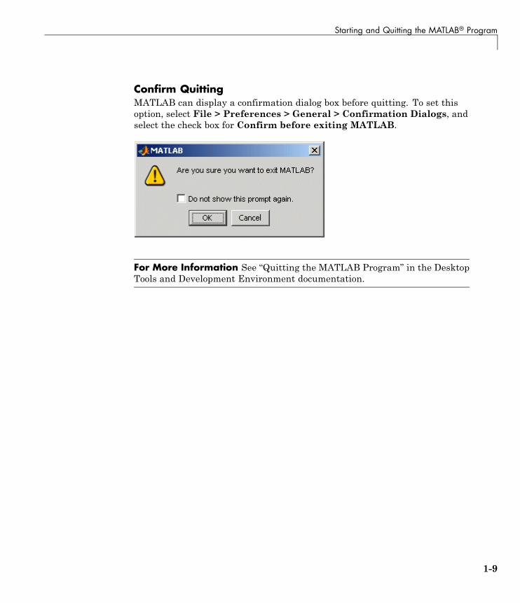
Confirm QuittingMATLAB can display a confirmation dialog box before quitting. To set thisoption, select File > Preferences > General > Confirmation Dialogs, andselect the check box for Confirm before exiting MATLAB.
For More Information See “Quitting the MATLAB Program” in the DesktopTools and Development Environment documentation.
1-9

1 Introduction
1-10
2
Matrices and Arrays
You can watch the Getting Started with MATLAB video demo for an overviewof the major functionality.
• “Matrices and Magic Squares” on page 2-2
• “Expressions” on page 2-11
• “Working with Matrices” on page 2-17
• “More About Matrices and Arrays” on page 2-21
• “Controlling Command Window Input and Output” on page 2-31
2 Matrices and Arrays
Matrices and Magic Squares
In this section...
“About Matrices” on page 2-2
“Entering Matrices” on page 2-4
“sum, transpose, and diag” on page 2-5
“Subscripts” on page 2-7
“The Colon Operator” on page 2-8
“The magic Function” on page 2-9
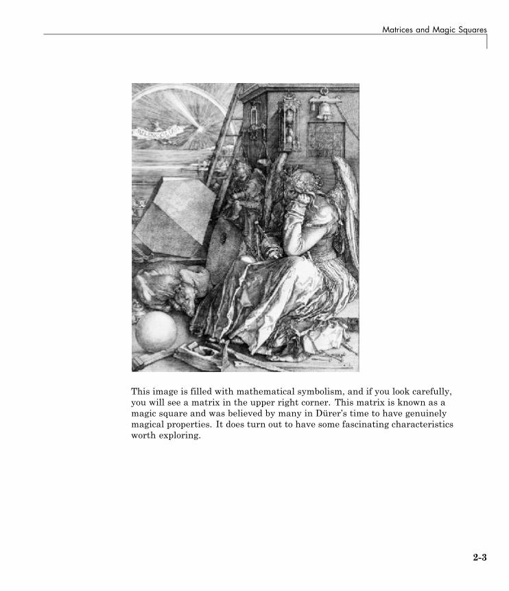
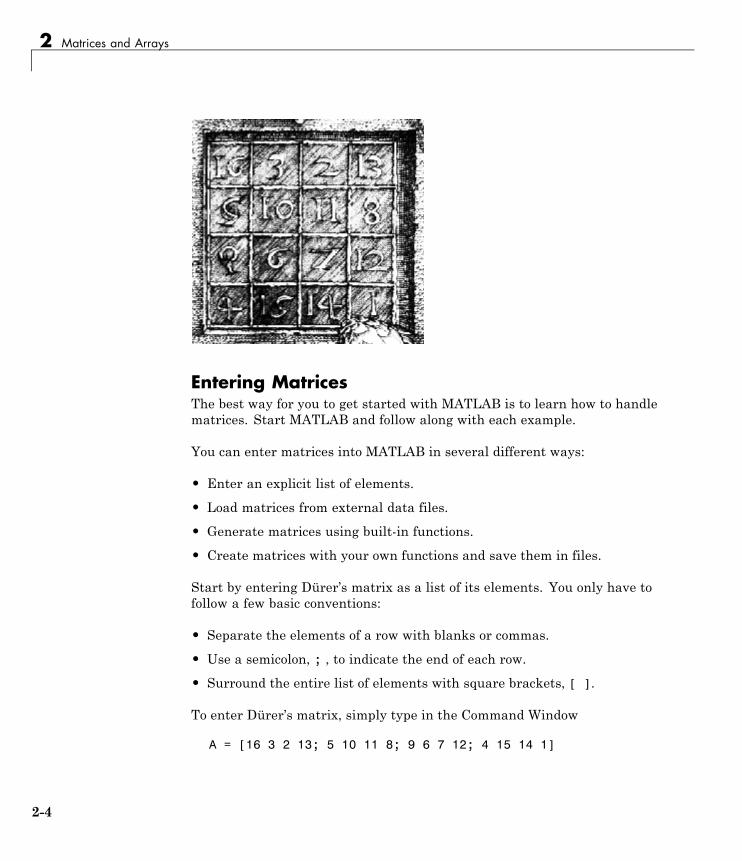
About MatricesIn the MATLAB environment, a matrix is a rectangular array of numbers.Special meaning is sometimes attached to 1-by-1 matrices, which arescalars, and to matrices with only one row or column, which are vectors.MATLAB has other ways of storing both numeric and nonnumeric data, butin the beginning, it is usually best to think of everything as a matrix. Theoperations in MATLAB are designed to be as natural as possible. Where otherprogramming languages work with numbers one at a time, MATLAB allowsyou to work with entire matrices quickly and easily. A good example matrix,used throughout this book, appears in the Renaissance engraving MelencoliaI by the German artist and amateur mathematician Albrecht Dürer.
2-2
Matrices and Magic Squares
This image is filled with mathematical symbolism, and if you look carefully,you will see a matrix in the upper right corner. This matrix is known as amagic square and was believed by many in Dürer’s time to have genuinelymagical properties. It does turn out to have some fascinating characteristicsworth exploring.
2-3
2 Matrices and Arrays
Entering MatricesThe best way for you to get started with MATLAB is to learn how to handlematrices. Start MATLAB and follow along with each example.
You can enter matrices into MATLAB in several different ways:
• Enter an explicit list of elements.
• Load matrices from external data files.
• Generate matrices using built-in functions.
• Create matrices with your own functions and save them in files.
Start by entering Dürer’s matrix as a list of its elements. You only have tofollow a few basic conventions:
• Separate the elements of a row with blanks or commas.
• Use a semicolon, ; , to indicate the end of each row.
• Surround the entire list of elements with square brackets, [ ].
To enter Dürer’s matrix, simply type in the Command Window
A = [16 3 2 13; 5 10 11 8; 9 6 7 12; 4 15 14 1]
2-4
Matrices and Magic Squares
MATLAB displays the matrix you just entered:
A =16 3 2 135 10 11 89 6 7 124 15 14 1
This matrix matches the numbers in the engraving. Once you have enteredthe matrix, it is automatically remembered in the MATLAB workspace. Youcan refer to it simply as A. Now that you have A in the workspace, take a lookat what makes it so interesting. Why is it magic?
sum, transpose, and diagYou are probably already aware that the special properties of a magic squarehave to do with the various ways of summing its elements. If you take thesum along any row or column, or along either of the two main diagonals,you will always get the same number. Let us verify that using MATLAB.The first statement to try is
sum(A)
MATLAB replies with
ans =34 34 34 34
When you do not specify an output variable, MATLAB uses the variable ans,short for answer, to store the results of a calculation. You have computed arow vector containing the sums of the columns of A. Each of the columns hasthe same sum, the magic sum, 34.
How about the row sums? MATLAB has a preference for working with thecolumns of a matrix, so one way to get the row sums is to transpose thematrix, compute the column sums of the transpose, and then transpose theresult. For an additional way that avoids the double transpose use thedimension argument for the sum function.
MATLAB has two transpose operators. The apostrophe operator (e.g., A')performs a complex conjugate transposition. It flips a matrix about its main
2-5
2 Matrices and Arrays
diagonal, and also changes the sign of the imaginary component of anycomplex elements of the matrix. The dot-apostrophe operator (e.g., A.'),transposes without affecting the sign of complex elements. For matricescontaining all real elements, the two operators return the same result.
So
A'
produces
ans =16 5 9 43 10 6 152 11 7 14
13 8 12 1
and
sum(A')'
produces a column vector containing the row sums
ans =34343434
The sum of the elements on the main diagonal is obtained with the sum andthe diag functions:
diag(A)
produces
ans =161071
2-6
Matrices and Magic Squares
and
sum(diag(A))
produces
ans =34
The other diagonal, the so-called antidiagonal, is not so importantmathematically, so MATLAB does not have a ready-made function for it.But a function originally intended for use in graphics, fliplr, flips a matrixfrom left to right:
sum(diag(fliplr(A)))ans =
34
You have verified that the matrix in Dürer’s engraving is indeed a magicsquare and, in the process, have sampled a few MATLAB matrix operations.The following sections continue to use this matrix to illustrate additionalMATLAB capabilities.
SubscriptsThe element in row i and column j of A is denoted by A(i,j). For example,A(4,2) is the number in the fourth row and second column. For the magicsquare, A(4,2) is 15. So to compute the sum of the elements in the fourthcolumn of A, type
A(1,4) + A(2,4) + A(3,4) + A(4,4)
This subscript produces
ans =34
but is not the most elegant way of summing a single column.
It is also possible to refer to the elements of a matrix with a single subscript,A(k). A single subscript is the usual way of referencing row and columnvectors. However, it can also apply to a fully two-dimensional matrix, in
2-7

2 Matrices and Arrays
which case the array is regarded as one long column vector formed from thecolumns of the original matrix. So, for the magic square, A(8) is another wayof referring to the value 15 stored in A(4,2).
If you try to use the value of an element outside of the matrix, it is an error:
t = A(4,5)Index exceeds matrix dimensions.
Conversely, if you store a value in an element outside of the matrix, the sizeincreases to accommodate the newcomer:
X = A;X(4,5) = 17
X =16 3 2 13 05 10 11 8 09 6 7 12 04 15 14 1 17
The Colon OperatorThe colon, :, is one of the most important MATLAB operators. It occurs inseveral different forms. The expression
1:10
is a row vector containing the integers from 1 to 10:
1 2 3 4 5 6 7 8 9 10
To obtain nonunit spacing, specify an increment. For example,
100:-7:50
is
100 93 86 79 72 65 58 51
and
0:pi/4:pi
2-8
Matrices and Magic Squares
is
0 0.7854 1.5708 2.3562 3.1416
Subscript expressions involving colons refer to portions of a matrix:
A(1:k,j)
is the first k elements of the jth column of A. Thus:
sum(A(1:4,4))
computes the sum of the fourth column. However, there is a better way toperform this computation. The colon by itself refers to all the elements ina row or column of a matrix and the keyword end refers to the last row orcolumn. Thus:
sum(A(:,end))
computes the sum of the elements in the last column of A:
ans =34
Why is the magic sum for a 4-by-4 square equal to 34? If the integers from 1to 16 are sorted into four groups with equal sums, that sum must be
sum(1:16)/4
which, of course, is
ans =34
The magic FunctionMATLAB actually has a built-in function that creates magic squares of almostany size. Not surprisingly, this function is named magic:
2-9

2 Matrices and Arrays
B = magic(4)B =
16 2 3 135 11 10 89 7 6 124 14 15 1
This matrix is almost the same as the one in the Dürer engraving and hasall the same “magic” properties; the only difference is that the two middlecolumns are exchanged.
To make this B into Dürer’s A, swap the two middle columns:
A = B(:,[1 3 2 4])
This subscript indicates that—for each of the rows of matrix B—reorder theelements in the order 1, 3, 2, 4. It produces:
A =16 3 2 135 10 11 89 6 7 124 15 14 1
2-10
Expressions
Expressions
In this section...
“Variables” on page 2-11
“Numbers” on page 2-12
“Operators” on page 2-13
“Functions” on page 2-14
“Examples of Expressions” on page 2-15
VariablesLike most other programming languages, the MATLAB language providesmathematical expressions, but unlike most programming languages, theseexpressions involve entire matrices.
MATLAB does not require any type declarations or dimension statements.When MATLAB encounters a new variable name, it automatically creates thevariable and allocates the appropriate amount of storage. If the variablealready exists, MATLAB changes its contents and, if necessary, allocatesnew storage. For example,
num_students = 25
creates a 1-by-1 matrix named num_students and stores the value 25 in itssingle element. To view the matrix assigned to any variable, simply enterthe variable name.
Variable names consist of a letter, followed by any number of letters, digits, orunderscores. MATLAB is case sensitive; it distinguishes between uppercaseand lowercase letters. A and a are not the same variable.
Although variable names can be of any length, MATLAB uses only the firstN characters of the name, (where N is the number returned by the functionnamelengthmax), and ignores the rest. Hence, it is important to makeeach variable name unique in the first N characters to enable MATLAB todistinguish variables.
2-11

2 Matrices and Arrays
N = namelengthmaxN =
63
The genvarname function can be useful in creating variable names that areboth valid and unique.
NumbersMATLAB uses conventional decimal notation, with an optional decimal pointand leading plus or minus sign, for numbers. Scientific notation uses theletter e to specify a power-of-ten scale factor. Imaginary numbers use either ior j as a suffix. Some examples of legal numbers are
3 -99 0.00019.6397238 1.60210e-20 6.02252e231i -3.14159j 3e5i
MATLAB stores all numbers internally using the long format specified bythe IEEE® floating-point standard. Floating-point numbers have a finiteprecision of roughly 16 significant decimal digits and a finite range of roughly10-308 to 10+308.
Numbers represented in the double format have a maximum precision of52 bits. Any double requiring more bits than 52 loses some precision. Forexample, the following code shows two unequal values to be equal becausethey are both truncated:
x = 36028797018963968;y = 36028797018963972;x == yans =
1
Integers have available precisions of 8-bit, 16-bit, 32-bit, and 64-bit. Storingthe same numbers as 64-bit integers preserves precision:
x = uint64(36028797018963968);y = uint64(36028797018963972);x == yans =
2-12
Expressions
0
The section “Avoiding Common Problems with Floating-Point Arithmetic”gives a few of the examples showing how IEEE floating-point arithmeticaffects computations in MATLAB. For more examples and information, seeTechnical Note 1108 — Common Problems with Floating-Point Arithmetic.
MATLAB software stores the real and imaginary parts of a complex number.It handles the magnitude of the parts in different ways depending on thecontext. For instance, the sort function sorts based on magnitude andresolves ties by phase angle.
sort([3+4i, 4+3i])ans =
4.0000 + 3.0000i 3.0000 + 4.0000i
This is because of the phase angle:
angle(3+4i)ans =
0.9273angle(4+3i)ans =
0.6435
The “equal to” relational operator == requires both the real and imaginaryparts to be equal. The other binary relational operators > <, >=, and <= ignorethe imaginary part of the number and consider the real part only.
OperatorsExpressions use familiar arithmetic operators and precedence rules.
+ Addition
- Subtraction
* Multiplication
/ Division
2-13
2 Matrices and Arrays
\ Left division (described in “Linear Algebra” in theMATLAB documentation)
^ Power
' Complex conjugate transpose
( ) Specify evaluation order
FunctionsMATLAB provides a large number of standard elementary mathematicalfunctions, including abs, sqrt, exp, and sin. Taking the square root orlogarithm of a negative number is not an error; the appropriate complex resultis produced automatically. MATLAB also provides many more advancedmathematical functions, including Bessel and gamma functions. Most ofthese functions accept complex arguments. For a list of the elementarymathematical functions, type
help elfun
For a list of more advanced mathematical and matrix functions, type
help specfunhelp elmat
Some of the functions, like sqrt and sin, are built in. Built-in functions arepart of the MATLAB core so they are very efficient, but the computationaldetails are not readily accessible. Other functions are implemented in theMATLAB programing language, so their computational details are accessible.
There are some differences between built-in functions and other functions.For example, for built-in functions, you cannot see the code. For otherfunctions, you can see the code and even modify it if you want.
Several special functions provide values of useful constants.
pi 3.14159265...
i Imaginary unit,
j Same as i
2-14
Expressions
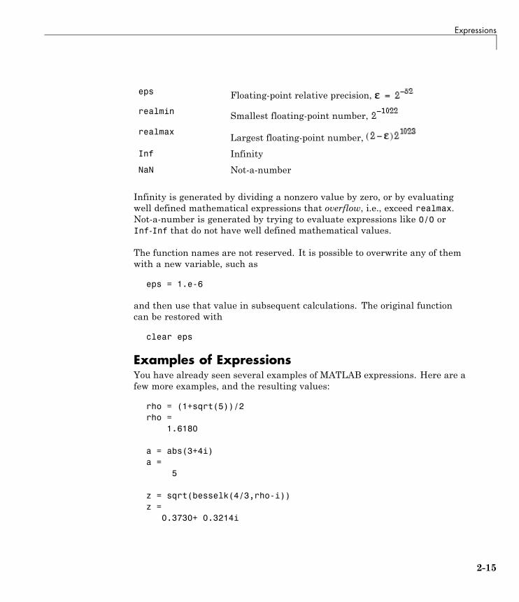
eps Floating-point relative precision,
realmin Smallest floating-point number,
realmaxLargest floating-point number,
Inf Infinity
NaN Not-a-number
Infinity is generated by dividing a nonzero value by zero, or by evaluatingwell defined mathematical expressions that overflow, i.e., exceed realmax.Not-a-number is generated by trying to evaluate expressions like 0/0 orInf-Inf that do not have well defined mathematical values.
The function names are not reserved. It is possible to overwrite any of themwith a new variable, such as
eps = 1.e-6
and then use that value in subsequent calculations. The original functioncan be restored with
clear eps
Examples of ExpressionsYou have already seen several examples of MATLAB expressions. Here are afew more examples, and the resulting values:
rho = (1+sqrt(5))/2rho =
1.6180
a = abs(3+4i)a =
5
z = sqrt(besselk(4/3,rho-i))z =
0.3730+ 0.3214i
2-15
2 Matrices and Arrays
huge = exp(log(realmax))huge =
1.7977e+308
toobig = pi*hugetoobig =
Inf
2-16
Working with Matrices
Working with Matrices
In this section...
“Generating Matrices” on page 2-17
“The load Function” on page 2-18
“Saving Code to a File” on page 2-18
“Concatenation” on page 2-19
“Deleting Rows and Columns” on page 2-20
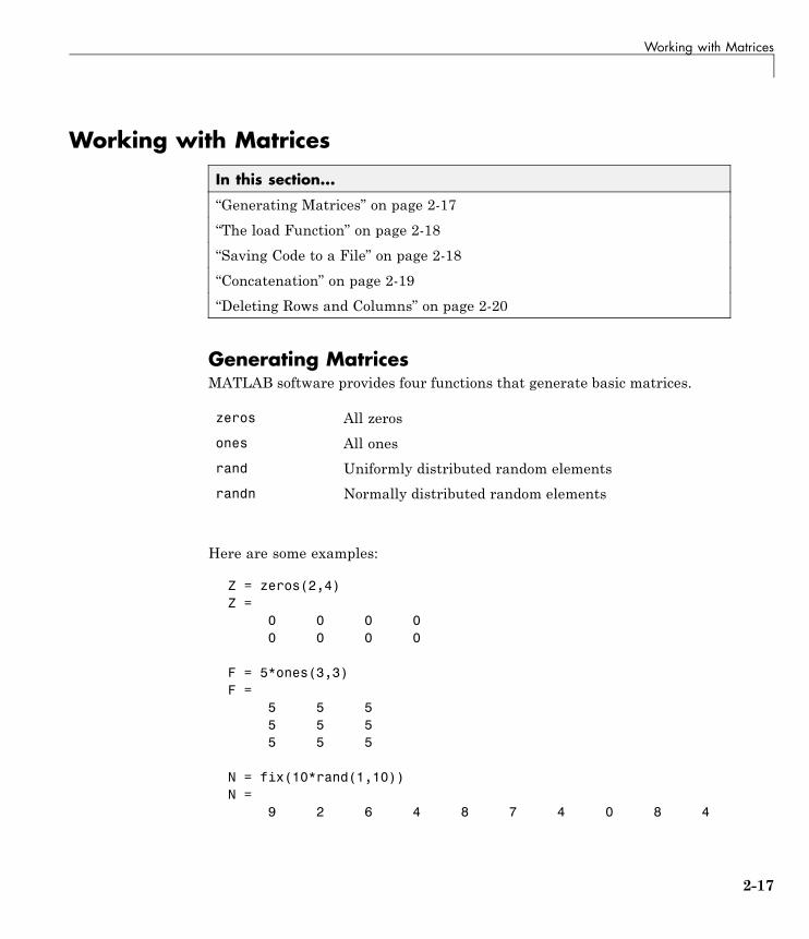
Generating MatricesMATLAB software provides four functions that generate basic matrices.
zeros All zeros
ones All ones
rand Uniformly distributed random elements
randn Normally distributed random elements
Here are some examples:
Z = zeros(2,4)Z =
0 0 0 00 0 0 0
F = 5*ones(3,3)F =
5 5 55 5 55 5 5
N = fix(10*rand(1,10))N =
9 2 6 4 8 7 4 0 8 4
2-17
2 Matrices and Arrays
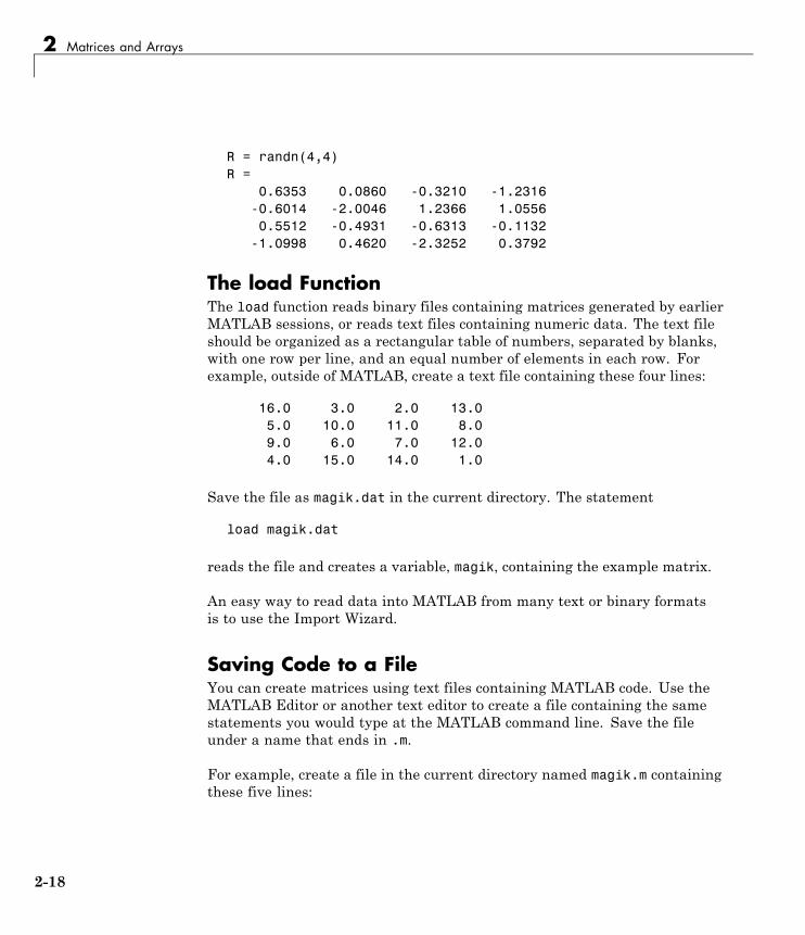
R = randn(4,4)R =
0.6353 0.0860 -0.3210 -1.2316-0.6014 -2.0046 1.2366 1.05560.5512 -0.4931 -0.6313 -0.1132
-1.0998 0.4620 -2.3252 0.3792
The load FunctionThe load function reads binary files containing matrices generated by earlierMATLAB sessions, or reads text files containing numeric data. The text fileshould be organized as a rectangular table of numbers, separated by blanks,with one row per line, and an equal number of elements in each row. Forexample, outside of MATLAB, create a text file containing these four lines:
16.0 3.0 2.0 13.05.0 10.0 11.0 8.09.0 6.0 7.0 12.04.0 15.0 14.0 1.0
Save the file as magik.dat in the current directory. The statement
load magik.dat
reads the file and creates a variable, magik, containing the example matrix.
An easy way to read data into MATLAB from many text or binary formatsis to use the Import Wizard.
Saving Code to a FileYou can create matrices using text files containing MATLAB code. Use theMATLAB Editor or another text editor to create a file containing the samestatements you would type at the MATLAB command line. Save the fileunder a name that ends in .m.
For example, create a file in the current directory named magik.m containingthese five lines:
2-18
Working with Matrices
A = [16.0 3.0 2.0 13.05.0 10.0 11.0 8.09.0 6.0 7.0 12.04.0 15.0 14.0 1.0 ];
The statement
magik
reads the file and creates a variable, A, containing the example matrix.
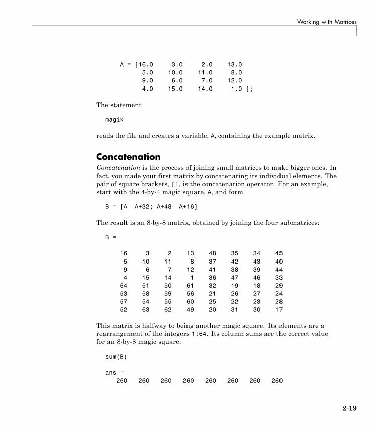
ConcatenationConcatenation is the process of joining small matrices to make bigger ones. Infact, you made your first matrix by concatenating its individual elements. Thepair of square brackets, [], is the concatenation operator. For an example,start with the 4-by-4 magic square, A, and form
B = [A A+32; A+48 A+16]
The result is an 8-by-8 matrix, obtained by joining the four submatrices:
B =
16 3 2 13 48 35 34 455 10 11 8 37 42 43 409 6 7 12 41 38 39 444 15 14 1 36 47 46 33
64 51 50 61 32 19 18 2953 58 59 56 21 26 27 2457 54 55 60 25 22 23 2852 63 62 49 20 31 30 17
This matrix is halfway to being another magic square. Its elements are arearrangement of the integers 1:64. Its column sums are the correct valuefor an 8-by-8 magic square:
sum(B)
ans =260 260 260 260 260 260 260 260
2-19
2 Matrices and Arrays
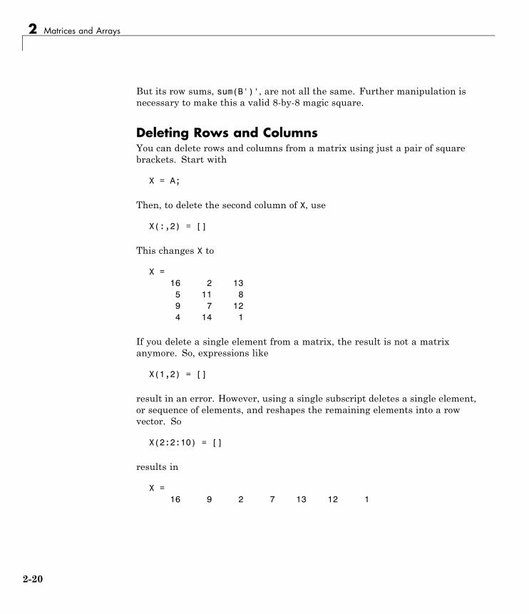
But its row sums, sum(B')', are not all the same. Further manipulation isnecessary to make this a valid 8-by-8 magic square.
Deleting Rows and ColumnsYou can delete rows and columns from a matrix using just a pair of squarebrackets. Start with
X = A;
Then, to delete the second column of X, use
X(:,2) = []
This changes X to
X =16 2 135 11 89 7 124 14 1
If you delete a single element from a matrix, the result is not a matrixanymore. So, expressions like
X(1,2) = []
result in an error. However, using a single subscript deletes a single element,or sequence of elements, and reshapes the remaining elements into a rowvector. So
X(2:2:10) = []
results in
X =16 9 2 7 13 12 1
2-20
More About Matrices and Arrays
More About Matrices and Arrays
In this section...
“Linear Algebra” on page 2-21
“Arrays” on page 2-25
“Multivariate Data” on page 2-27
“Scalar Expansion” on page 2-28
“Logical Subscripting” on page 2-28
“The find Function” on page 2-29
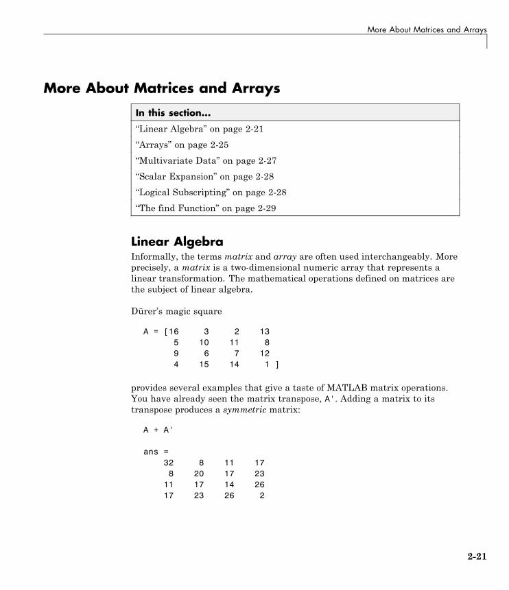
Linear AlgebraInformally, the terms matrix and array are often used interchangeably. Moreprecisely, a matrix is a two-dimensional numeric array that represents alinear transformation. The mathematical operations defined on matrices arethe subject of linear algebra.
Dürer’s magic square
A = [16 3 2 135 10 11 89 6 7 124 15 14 1 ]
provides several examples that give a taste of MATLAB matrix operations.You have already seen the matrix transpose, A'. Adding a matrix to itstranspose produces a symmetric matrix:
A + A'
ans =32 8 11 178 20 17 23
11 17 14 2617 23 26 2
2-21
2 Matrices and Arrays
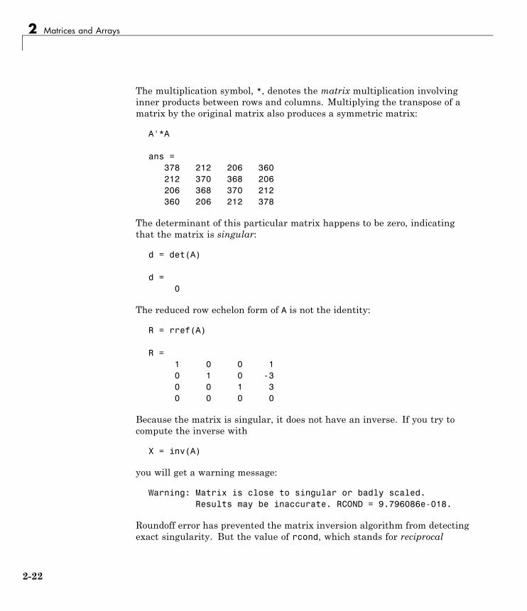
The multiplication symbol, *, denotes the matrix multiplication involvinginner products between rows and columns. Multiplying the transpose of amatrix by the original matrix also produces a symmetric matrix:
A'*A
ans =378 212 206 360212 370 368 206206 368 370 212360 206 212 378
The determinant of this particular matrix happens to be zero, indicatingthat the matrix is singular:
d = det(A)
d =0
The reduced row echelon form of A is not the identity:
R = rref(A)
R =1 0 0 10 1 0 -30 0 1 30 0 0 0
Because the matrix is singular, it does not have an inverse. If you try tocompute the inverse with
X = inv(A)
you will get a warning message:
Warning: Matrix is close to singular or badly scaled.Results may be inaccurate. RCOND = 9.796086e-018.
Roundoff error has prevented the matrix inversion algorithm from detectingexact singularity. But the value of rcond, which stands for reciprocal
2-22
More About Matrices and Arrays
condition estimate, is on the order of eps, the floating-point relative precision,so the computed inverse is unlikely to be of much use.
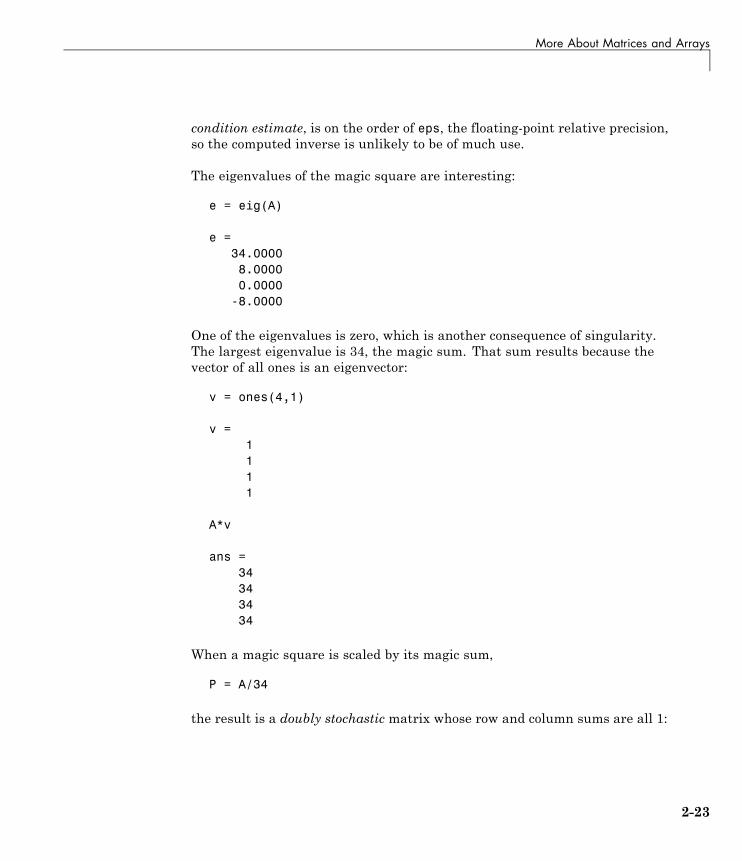
The eigenvalues of the magic square are interesting:
e = eig(A)
e =34.00008.00000.0000
-8.0000
One of the eigenvalues is zero, which is another consequence of singularity.The largest eigenvalue is 34, the magic sum. That sum results because thevector of all ones is an eigenvector:
v = ones(4,1)
v =1111
A*v
ans =34343434
When a magic square is scaled by its magic sum,
P = A/34
the result is a doubly stochastic matrix whose row and column sums are all 1:
2-23
2 Matrices and Arrays
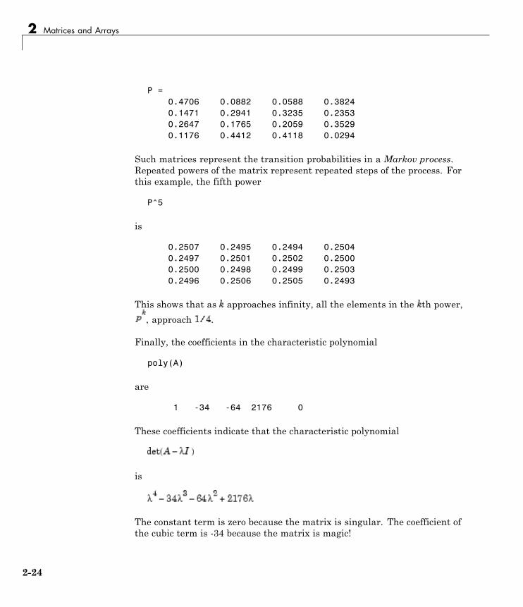
P =0.4706 0.0882 0.0588 0.38240.1471 0.2941 0.3235 0.23530.2647 0.1765 0.2059 0.35290.1176 0.4412 0.4118 0.0294
Such matrices represent the transition probabilities in a Markov process.Repeated powers of the matrix represent repeated steps of the process. Forthis example, the fifth power
P^5
is
0.2507 0.2495 0.2494 0.25040.2497 0.2501 0.2502 0.25000.2500 0.2498 0.2499 0.25030.2496 0.2506 0.2505 0.2493
This shows that as approaches infinity, all the elements in the th power,
, approach .
Finally, the coefficients in the characteristic polynomial
poly(A)
are
1 -34 -64 2176 0
These coefficients indicate that the characteristic polynomial
is
The constant term is zero because the matrix is singular. The coefficient ofthe cubic term is -34 because the matrix is magic!
2-24

More About Matrices and Arrays
ArraysWhen they are taken away from the world of linear algebra, matrices becometwo-dimensional numeric arrays. Arithmetic operations on arrays aredone element by element. This means that addition and subtraction arethe same for arrays and matrices, but that multiplicative operations aredifferent. MATLAB uses a dot, or decimal point, as part of the notation formultiplicative array operations.
The list of operators includes
+ Addition
- Subtraction
.* Element-by-element multiplication
./ Element-by-element division
.\ Element-by-element left division
.^ Element-by-element power
.' Unconjugated array transpose
If the Dürer magic square is multiplied by itself with array multiplication
A.*A
the result is an array containing the squares of the integers from 1 to 16,in an unusual order:
ans =256 9 4 16925 100 121 6481 36 49 14416 225 196 1
Building TablesArray operations are useful for building tables. Suppose n is the column vector
n = (0:9)';
2-25
2 Matrices and Arrays
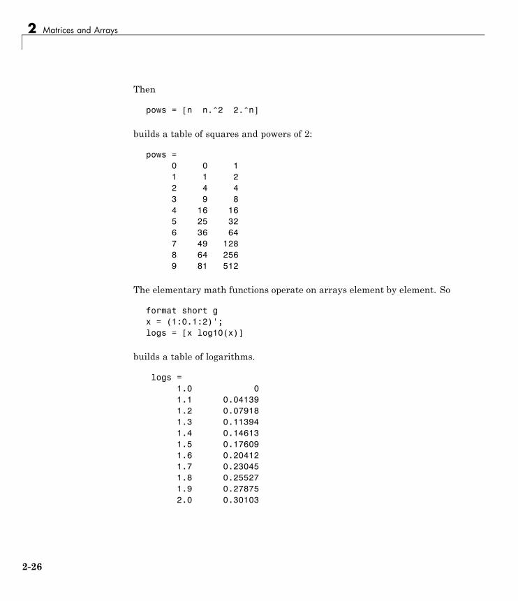
Then
pows = [n n.^2 2.^n]
builds a table of squares and powers of 2:
pows =0 0 11 1 22 4 43 9 84 16 165 25 326 36 647 49 1288 64 2569 81 512
The elementary math functions operate on arrays element by element. So
format short gx = (1:0.1:2)';logs = [x log10(x)]
builds a table of logarithms.
logs =1.0 01.1 0.041391.2 0.079181.3 0.113941.4 0.146131.5 0.176091.6 0.204121.7 0.230451.8 0.255271.9 0.278752.0 0.30103
2-26
More About Matrices and Arrays
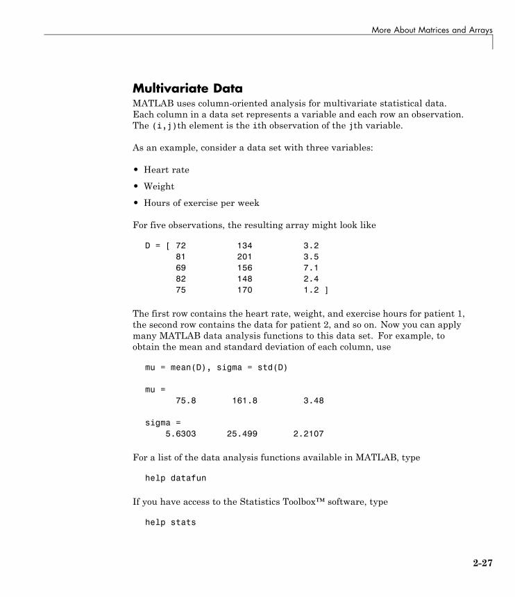
Multivariate DataMATLAB uses column-oriented analysis for multivariate statistical data.Each column in a data set represents a variable and each row an observation.The (i,j)th element is the ith observation of the jth variable.
As an example, consider a data set with three variables:
• Heart rate
• Weight
• Hours of exercise per week
For five observations, the resulting array might look like
D = [ 72 134 3.281 201 3.569 156 7.182 148 2.475 170 1.2 ]
The first row contains the heart rate, weight, and exercise hours for patient 1,the second row contains the data for patient 2, and so on. Now you can applymany MATLAB data analysis functions to this data set. For example, toobtain the mean and standard deviation of each column, use
mu = mean(D), sigma = std(D)
mu =75.8 161.8 3.48
sigma =5.6303 25.499 2.2107
For a list of the data analysis functions available in MATLAB, type
help datafun
If you have access to the Statistics Toolbox™ software, type
help stats
2-27
2 Matrices and Arrays
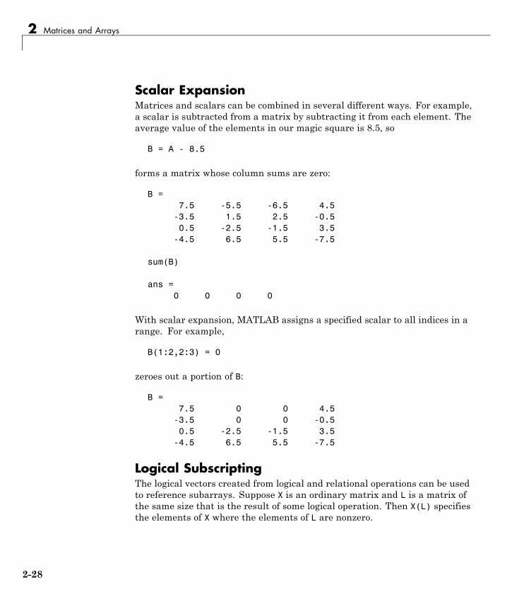
Scalar ExpansionMatrices and scalars can be combined in several different ways. For example,a scalar is subtracted from a matrix by subtracting it from each element. Theaverage value of the elements in our magic square is 8.5, so
B = A - 8.5
forms a matrix whose column sums are zero:
B =7.5 -5.5 -6.5 4.5
-3.5 1.5 2.5 -0.50.5 -2.5 -1.5 3.5
-4.5 6.5 5.5 -7.5
sum(B)
ans =0 0 0 0
With scalar expansion, MATLAB assigns a specified scalar to all indices in arange. For example,
B(1:2,2:3) = 0
zeroes out a portion of B:
B =7.5 0 0 4.5
-3.5 0 0 -0.50.5 -2.5 -1.5 3.5
-4.5 6.5 5.5 -7.5
Logical SubscriptingThe logical vectors created from logical and relational operations can be usedto reference subarrays. Suppose X is an ordinary matrix and L is a matrix ofthe same size that is the result of some logical operation. Then X(L) specifiesthe elements of X where the elements of L are nonzero.
2-28
More About Matrices and Arrays
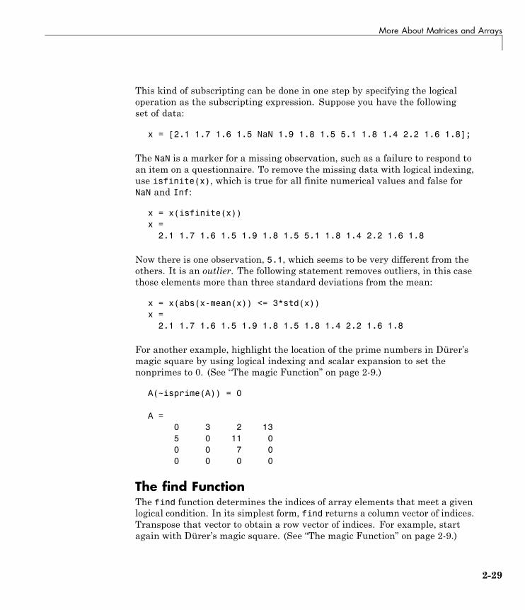
This kind of subscripting can be done in one step by specifying the logicaloperation as the subscripting expression. Suppose you have the followingset of data:
x = [2.1 1.7 1.6 1.5 NaN 1.9 1.8 1.5 5.1 1.8 1.4 2.2 1.6 1.8];
The NaN is a marker for a missing observation, such as a failure to respond toan item on a questionnaire. To remove the missing data with logical indexing,use isfinite(x), which is true for all finite numerical values and false forNaN and Inf:
x = x(isfinite(x))x =
2.1 1.7 1.6 1.5 1.9 1.8 1.5 5.1 1.8 1.4 2.2 1.6 1.8
Now there is one observation, 5.1, which seems to be very different from theothers. It is an outlier. The following statement removes outliers, in this casethose elements more than three standard deviations from the mean:
x = x(abs(x-mean(x)) <= 3*std(x))x =
2.1 1.7 1.6 1.5 1.9 1.8 1.5 1.8 1.4 2.2 1.6 1.8
For another example, highlight the location of the prime numbers in Dürer’smagic square by using logical indexing and scalar expansion to set thenonprimes to 0. (See “The magic Function” on page 2-9.)
A(~isprime(A)) = 0
A =0 3 2 135 0 11 00 0 7 00 0 0 0
The find FunctionThe find function determines the indices of array elements that meet a givenlogical condition. In its simplest form, find returns a column vector of indices.Transpose that vector to obtain a row vector of indices. For example, startagain with Dürer’s magic square. (See “The magic Function” on page 2-9.)
2-29
2 Matrices and Arrays
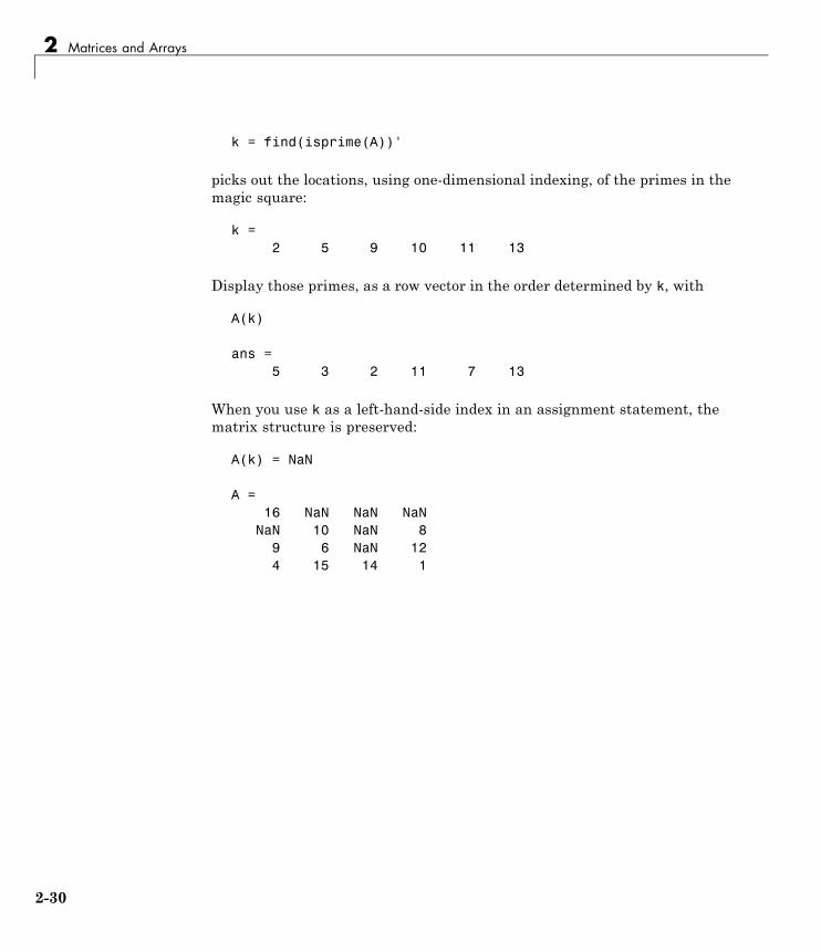
k = find(isprime(A))'
picks out the locations, using one-dimensional indexing, of the primes in themagic square:
k =2 5 9 10 11 13
Display those primes, as a row vector in the order determined by k, with
A(k)
ans =5 3 2 11 7 13
When you use k as a left-hand-side index in an assignment statement, thematrix structure is preserved:
A(k) = NaN
A =16 NaN NaN NaN
NaN 10 NaN 89 6 NaN 124 15 14 1
2-30

Controlling Command Window Input and Output
Controlling Command Window Input and Output
In this section...
“The format Function” on page 2-31
“Suppressing Output” on page 2-32
“Entering Long Statements” on page 2-33
“Command Line Editing” on page 2-33
The format FunctionThe format function controls the numeric format of the values displayed. Thefunction affects only how numbers are displayed, not how MATLAB softwarecomputes or saves them. Here are the different formats, together with theresulting output produced from a vector x with components of differentmagnitudes.
Note To ensure proper spacing, use a fixed-width font, such as Courier.
x = [4/3 1.2345e-6]
format short
1.3333 0.0000
format short e
1.3333e+000 1.2345e-006
format short g
1.3333 1.2345e-006
format long
1.33333333333333 0.00000123450000
2-31
2 Matrices and Arrays
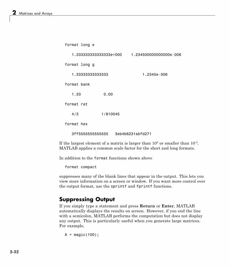
format long e
1.333333333333333e+000 1.234500000000000e-006
format long g
1.33333333333333 1.2345e-006
format bank
1.33 0.00
format rat
4/3 1/810045
format hex
3ff5555555555555 3eb4b6231abfd271
If the largest element of a matrix is larger than 103 or smaller than 10-3,MATLAB applies a common scale factor for the short and long formats.
In addition to the format functions shown above
format compact
suppresses many of the blank lines that appear in the output. This lets youview more information on a screen or window. If you want more control overthe output format, use the sprintf and fprintf functions.
Suppressing OutputIf you simply type a statement and press Return or Enter, MATLABautomatically displays the results on screen. However, if you end the linewith a semicolon, MATLAB performs the computation but does not displayany output. This is particularly useful when you generate large matrices.For example,
A = magic(100);
2-32

Controlling Command Window Input and Output
Entering Long StatementsIf a statement does not fit on one line, use an ellipsis (three periods), ...,followed by Return or Enter to indicate that the statement continues onthe next line. For example,
s = 1 -1/2 + 1/3 -1/4 + 1/5 - 1/6 + 1/7 ...- 1/8 + 1/9 - 1/10 + 1/11 - 1/12;
Blank spaces around the =, +, and - signs are optional, but they improvereadability.
Command Line EditingVarious arrow and control keys on your keyboard allow you to recall, edit,and reuse statements you have typed earlier. For example, suppose youmistakenly enter
rho = (1 + sqt(5))/2
You have misspelled sqrt. MATLAB responds with
Undefined function or method 'sqt' for input arguments of type 'double'.
Instead of retyping the entire line, simply press the key. The statementyou typed is redisplayed. Use the key to move the cursor over and insertthe missing r. Repeated use of the key recalls earlier lines. Typing a fewcharacters and then the key finds a previous line that begins with thosecharacters. You can also copy previously executed statements from theCommand History. For more information, see “Command History” on page7-6.
2-33

2 Matrices and Arrays
2-34
3
Graphics
• “Overview of Plotting” on page 3-2
• “Editing Plots” on page 3-24
• “Some Ways to Use Plotting Tools” on page 3-30
• “Preparing Graphs for Presentation” on page 3-44
• “Using Basic Plotting Functions” on page 3-57
• “Creating Mesh and Surface Plots” on page 3-72
• “Plotting Image Data” on page 3-80
• “Printing Graphics” on page 3-82
• “Understanding Handle Graphics Objects” on page 3-85
3 Graphics
Overview of Plotting
In this section...
“Plotting Process” on page 3-2
“Graph Components” on page 3-6
“Figure Tools” on page 3-7
“Arranging Graphs Within a Figure” on page 3-14
“Choosing a Type of Graph to Plot” on page 3-15
For More Information See MATLAB Graphics and 3-D Visualization in theMATLAB documentation for in-depth coverage of MATLAB graphics andvisualization tools. Access these topics from the Help browser.
Plotting ProcessThe MATLAB environment provides a wide variety of techniques to displaydata graphically. Interactive tools enable you to manipulate graphs to achieveresults that reveal the most information about your data. You can alsoannotate and print graphs for presentations, or export graphs to standardgraphics formats for presentation in Web browsers or other media.
The process of visualizing data typically involves a series of operations. Thissection provides a “big picture” view of the plotting process and containslinks to sections that have examples and specific details about performingeach operation.
Creating a GraphThe type of graph you choose to create depends on the nature of your dataand what you want to reveal about the data. You can choose from manypredefined graph types, such as line, bar, histogram, and pie graphs as wellas 3-D graphs, such as surfaces, slice planes, and streamlines.
There are two basic ways to create MATLAB graphs:
• Use plotting tools to create graphs interactively.
3-2
Overview of Plotting
See “Some Ways to Use Plotting Tools” on page 3-30.
• Use the command interface to enter commands in the Command Windowor create plotting programs.
See “Using Basic Plotting Functions” on page 3-57.
You might find it useful to combine both approaches. For example, you mightissue a plotting command to create a graph and then modify the graph usingone of the interactive tools.
Exploring DataAfter you create a graph, you can extract specific information about the data,such as the numeric value of a peak in a plot, the average value of a series ofdata, or you can perform data fitting. You can also identify individual graphobservations with Datatip and Data brushing tools and trace them back totheir data sources in the MATLAB workspace.
For More Information See “Data Exploration Tools” in the MATLABGraphics documentation and “Marking Up Graphs with Data Brushing”,“Making Graphs Responsive with Data Linking”, “Interacting with GraphedData”, and “Opening the Basic Fitting GUI” in the MATLAB Data Analysisdocumentation.
Editing the Graph ComponentsGraphs are composed of objects, which have properties you can change. Theseproperties affect the way the various graph components look and behave.
For example, the axes used to define the coordinate system of the graph hasproperties that define the limits of each axis, the scale, color, etc. The lineused to create a line graph has properties such as color, type of marker usedat each data point (if any), line style, etc.
3-3
3 Graphics
Note The data values that a line graph (for example) displays are copied intoand become properties of the (lineseries) graphics object. You can, therefore,change the data in the workspace without creating a new graph. You can alsoadd data to a graph. See “Editing Plots” on page 3-24 for more information.
Annotating GraphsAnnotations are the text, arrows, callouts, and other labels added to graphsto help viewers see what is important about the data. You typically addannotations to graphs when you want to show them to other people or whenyou want to save them for later reference.
For More Information See “Annotating Graphs” in the MATLAB Graphicsdocumentation, or select Annotating Graphs from the figure Help menu.
Printing and Exporting GraphsYou can print your graph on any printer connected to your computer. Theprint previewer enables you to view how your graph will look when printed.It enables you to add headers, footers, a date, and so on. The print previewdialog box lets you control the size, layout, and other characteristics of thegraph (select Print Preview from the figure File menu).
Exporting a graph means creating a copy of it in a standard graphics fileformat, such as TIFF, JPEG, or EPS. You can then import the file into a wordprocessor, include it in an HTML document, or edit it in a drawing package(select Export Setup from the figure File menu).
Adding and Removing Figure ContentBy default, when you create a new graph in the same figure window, its datareplaces that of the graph that is currently displayed, if any. You can addnew data to a graph in several ways; see “Adding More Data to the Graph”on page 3-34 for how to do this using a GUI. You can manually remove alldata, graphics and annotations from the current figure by typing clf in theCommand Window or by selecting Clear Figure from the figure’s Edit menu.
3-4
Overview of Plotting
For More Information See the print command reference page and “Printingand Exporting” in the MATLAB Graphics documentation, or select Printingand Exporting from the figure Help menu.
Saving Graphs for ReuseThere are two ways to save graphs that enable you to save the work youhave invested in their preparation:
• Save the graph as a FIG-file (select Save from the figure File menu).
• Generate MATLAB code that can recreate the graph (select Generatecode from the figure File menu).
FIG-Files. FIG-files are a binary format that saves a figure in its currentstate. This means that all graphics objects and property settings are stored inthe file when you create it. You can reload the file into a different MATLABsession, even when you run it on a different type of computer. When you load aFIG-file, a new MATLAB figure opens in the same state as the one you saved.
Note The states of any figure tools on the toolbars are not saved in a FIG-file;only the contents of the graph and its annotations are saved. The contents ofdatatips (created by the Data Cursor tool), are also saved. This means thatFIG-files always open in the default figure mode.
Generated Code. You can use the MATLAB code generator to create codethat recreates the graph. Unlike a FIG-file, the generated code does notcontain any data. You must pass appropriate data to the generated functionwhen you run the code.
Studying the generated code for a graph is a good way to learn how to programusing MATLAB.
For More Information See the print command reference page and “SavingYour Work” in the MATLAB Graphics documentation.
3-5
3 Graphics
Graph ComponentsMATLAB graphs display in a special window known as a figure. To createa graph, you need to define a coordinate system. Therefore, every graph isplaced within axes, which are contained by the figure.
You achieve the actual visual representation of the data with graphics objectslike lines and surfaces. These objects are drawn within the coordinate systemdefined by the axes, which appear automatically to specifically span the rangeof the data. The actual data is stored as properties of the graphics objects.
See “Understanding Handle Graphics Objects” on page 3-85 for moreinformation about graphics object properties.
The following picture shows the basic components of a typical graph. You canfind commands for plotting this graph in “Preparing Graphs for Presentation”on page 3-44.
3-6

Overview of Plotting
!� ���������������� �� �����
�"��������������������� ����������� ����
������������������������
����#�������� �������������������������������
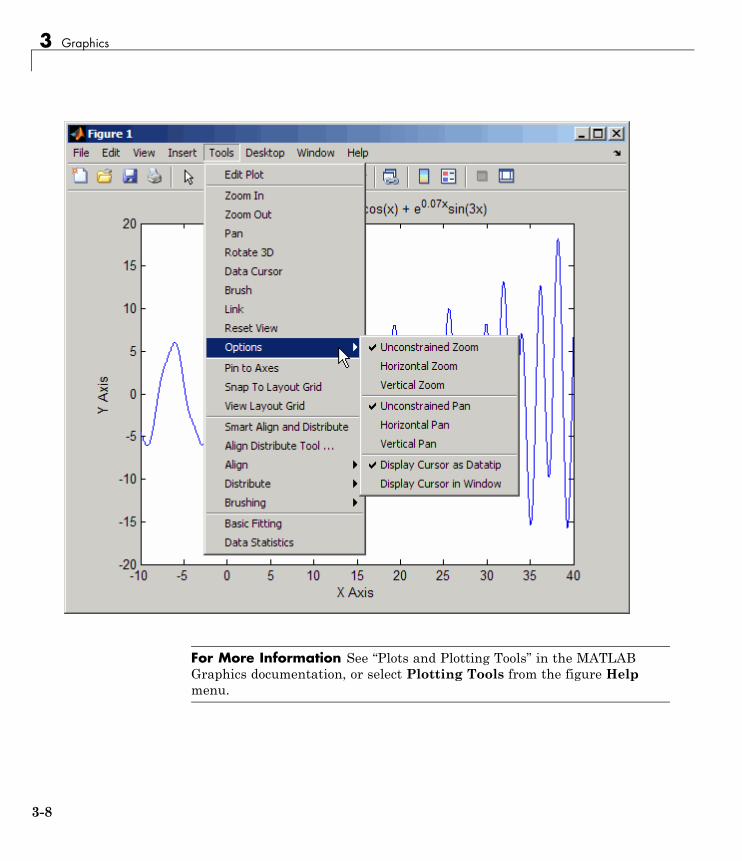
Figure ToolsThe figure is equipped with sets of tools that operate on graphs. The figureTools menu provides access to many graph tools, as this view of the Optionssubmenu illustrates. Many of the options shown in this figure also appear ascontext menu items for individual tools such as zoom and pan. The figure alsoshows three figure toolbars, discussed in “Figure Toolbars” on page 3-9.
3-7
3 Graphics
For More Information See “Plots and Plotting Tools” in the MATLABGraphics documentation, or select Plotting Tools from the figure Helpmenu.
3-8
Overview of Plotting
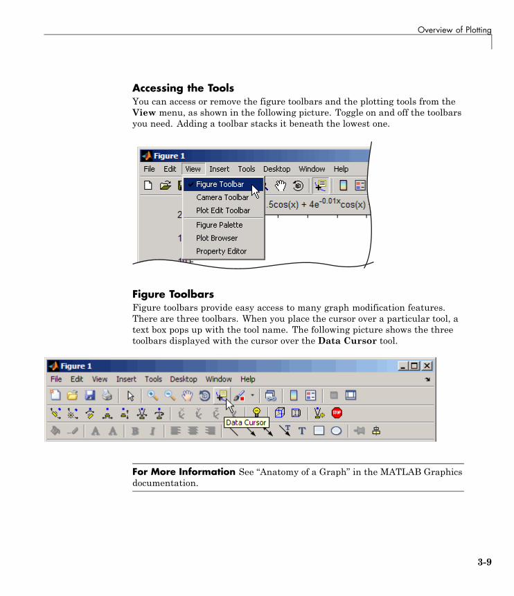
Accessing the ToolsYou can access or remove the figure toolbars and the plotting tools from theView menu, as shown in the following picture. Toggle on and off the toolbarsyou need. Adding a toolbar stacks it beneath the lowest one.
Figure ToolbarsFigure toolbars provide easy access to many graph modification features.There are three toolbars. When you place the cursor over a particular tool, atext box pops up with the tool name. The following picture shows the threetoolbars displayed with the cursor over the Data Cursor tool.
For More Information See “Anatomy of a Graph” in the MATLAB Graphicsdocumentation.
3-9
3 Graphics
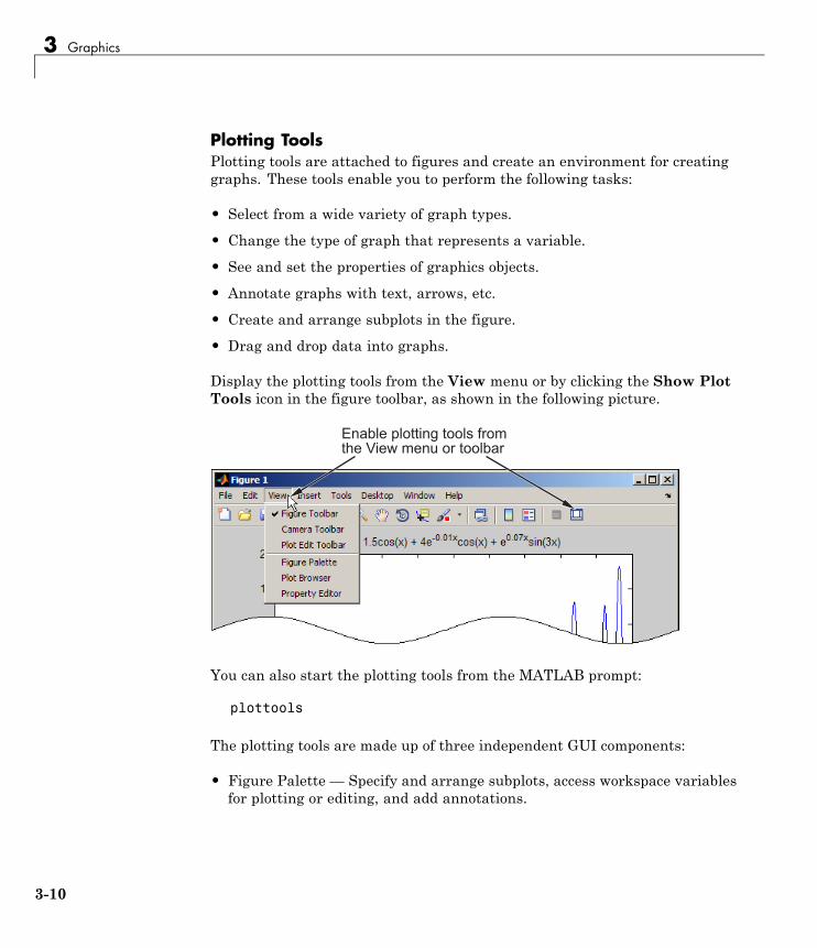
Plotting ToolsPlotting tools are attached to figures and create an environment for creatinggraphs. These tools enable you to perform the following tasks:
• Select from a wide variety of graph types.
• Change the type of graph that represents a variable.
• See and set the properties of graphics objects.
• Annotate graphs with text, arrows, etc.
• Create and arrange subplots in the figure.
• Drag and drop data into graphs.
Display the plotting tools from the View menu or by clicking the Show PlotTools icon in the figure toolbar, as shown in the following picture.
���#���������� �������������������������������#��
You can also start the plotting tools from the MATLAB prompt:
plottools
The plotting tools are made up of three independent GUI components:
• Figure Palette — Specify and arrange subplots, access workspace variablesfor plotting or editing, and add annotations.
3-10
Overview of Plotting
• Plot Browser — Select objects in the graphics hierarchy, control visibility,and add data to axes.
• Property Editor — Change key properties of the selected object. ClickMoreProperties to access all object properties with the Property Inspector.
You can also control these components from the Command Window, by typingthe following:
figurepaletteplotbrowserpropertyeditor
See the reference pages for plottools, figurepalette, plotbrowser, andpropertyeditor for information on syntax and options.
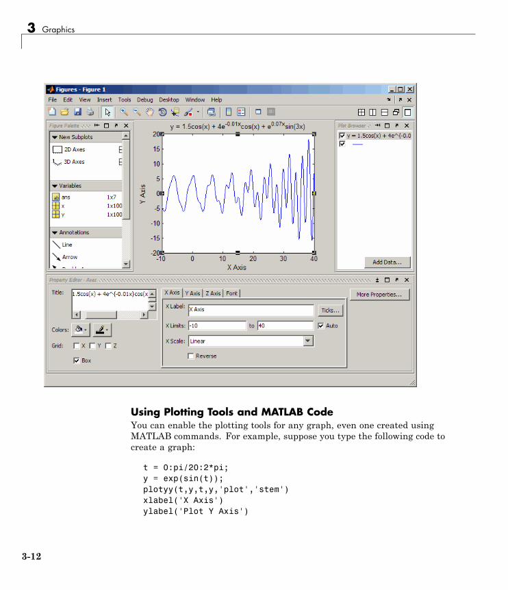
The following picture shows a figure with all three plotting tools enabled.
3-11
3 Graphics
Using Plotting Tools and MATLAB CodeYou can enable the plotting tools for any graph, even one created usingMATLAB commands. For example, suppose you type the following code tocreate a graph:
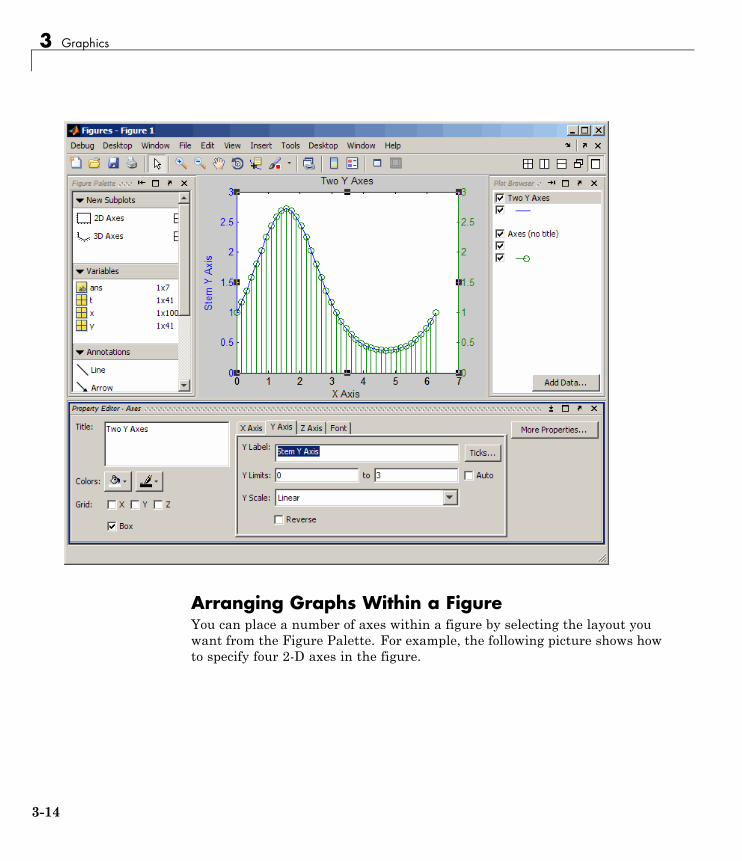
t = 0:pi/20:2*pi;y = exp(sin(t));plotyy(t,y,t,y,'plot','stem')xlabel('X Axis')ylabel('Plot Y Axis')
3-12
Overview of Plotting
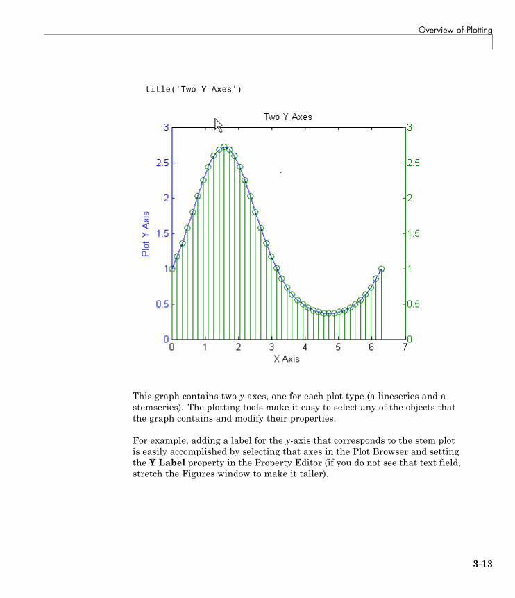
title('Two Y Axes')
This graph contains two y-axes, one for each plot type (a lineseries and astemseries). The plotting tools make it easy to select any of the objects thatthe graph contains and modify their properties.
For example, adding a label for the y-axis that corresponds to the stem plotis easily accomplished by selecting that axes in the Plot Browser and settingthe Y Label property in the Property Editor (if you do not see that text field,stretch the Figures window to make it taller).
3-13
3 Graphics
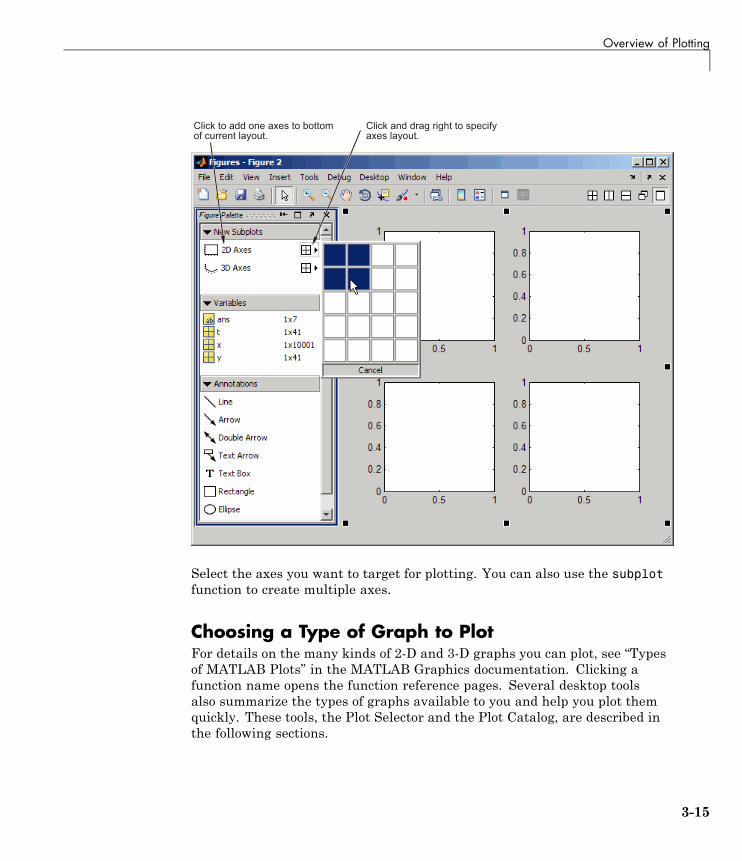
Arranging Graphs Within a FigureYou can place a number of axes within a figure by selecting the layout youwant from the Figure Palette. For example, the following picture shows howto specify four 2-D axes in the figure.
3-14
Overview of Plotting
$��%�������������"������#����������������� ����
$��%�������� ��� ���������� �"����� ����
Select the axes you want to target for plotting. You can also use the subplotfunction to create multiple axes.
Choosing a Type of Graph to PlotFor details on the many kinds of 2-D and 3-D graphs you can plot, see “Typesof MATLAB Plots” in the MATLAB Graphics documentation. Clicking afunction name opens the function reference pages. Several desktop toolsalso summarize the types of graphs available to you and help you plot themquickly. These tools, the Plot Selector and the Plot Catalog, are described inthe following sections.
3-15
3 Graphics
Creating Graphs with the Plot SelectorAfter you select variables in the Workspace Browser, you can create a graph
of the data by clicking the Plot Selector toolbar button. The PlotSelector icon depicts the type of graph it creates by default. The default graphreflects the variables you select and your history of using the tool. The PlotSelector icon changes to indicate the default type of graph along with thefunction’s name and calling arguments. If you click the icon, the Plot Selectorexecutes that code to create a graph of the type it displays. For example,when you select two vectors named t and y, the Plot Selector initially displaysplot(t,y).
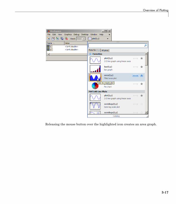
If you click the down-arrow on the right side of the button, its menu opens todisplay all graph types compatible with the selected variables. The followingfigure shows the Plot Selector menu with an area graph selected. The graphtypes that the Plot Selector shows as available are consistent with thevariables (t and y) currently selected in the Workspace Browser.
3-16
Overview of Plotting
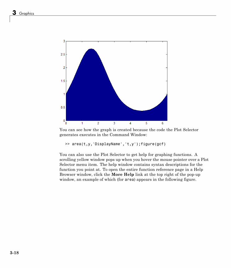
Releasing the mouse button over the highlighted icon creates an area graph.
3-17
3 Graphics
You can see how the graph is created because the code the Plot Selectorgenerates executes in the Command Window:
>> area(t,y,'DisplayName','t,y');figure(gcf)
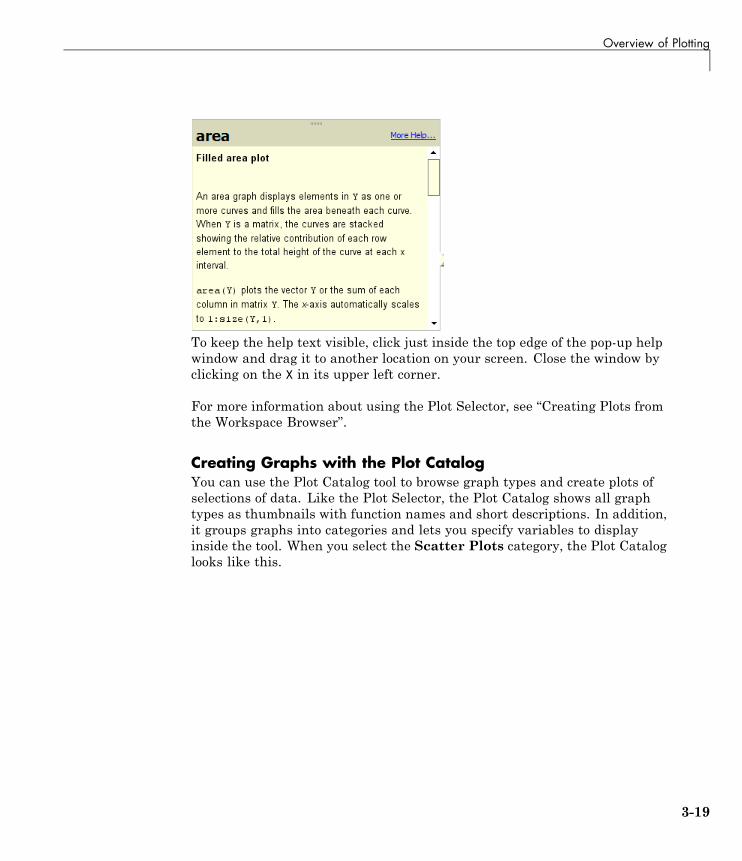
You can also use the Plot Selector to get help for graphing functions. Ascrolling yellow window pops up when you hover the mouse pointer over a PlotSelector menu item. The help window contains syntax descriptions for thefunction you point at. To open the entire function reference page in a HelpBrowser window, click the More Help link at the top right of the pop-upwindow, an example of which (for area) appears in the following figure.
3-18
Overview of Plotting
To keep the help text visible, click just inside the top edge of the pop-up helpwindow and drag it to another location on your screen. Close the window byclicking on the X in its upper left corner.
For more information about using the Plot Selector, see “Creating Plots fromthe Workspace Browser”.
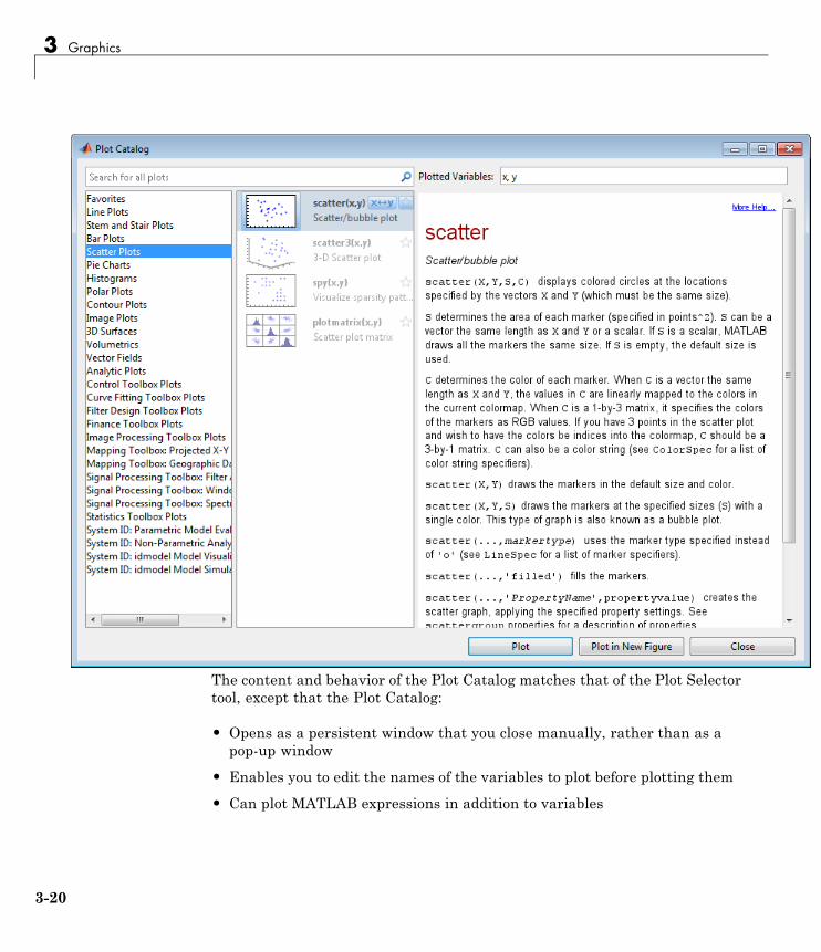
Creating Graphs with the Plot CatalogYou can use the Plot Catalog tool to browse graph types and create plots ofselections of data. Like the Plot Selector, the Plot Catalog shows all graphtypes as thumbnails with function names and short descriptions. In addition,it groups graphs into categories and lets you specify variables to displayinside the tool. When you select the Scatter Plots category, the Plot Cataloglooks like this.
3-19
3 Graphics
The content and behavior of the Plot Catalog matches that of the Plot Selectortool, except that the Plot Catalog:
• Opens as a persistent window that you close manually, rather than as apop-up window
• Enables you to edit the names of the variables to plot before plotting them
• Can plot MATLAB expressions in addition to variables
3-20
Overview of Plotting
• Provides help for the selected graph type in the right pane, rather thanin a pop-up window.
Open the Plot Catalog in any of the following ways:
• From the Plot Selector menu in the Workspace browser or Variable Editor,click the Catalog link at the bottom of the menu.
• In the Workspace browser, right-click a variable and choose Plot Catalogfrom the context menu.
• In the Variable Editor, select the values you want to graph, right-click theselection you just made, and choose Plot Catalog from the context menu.
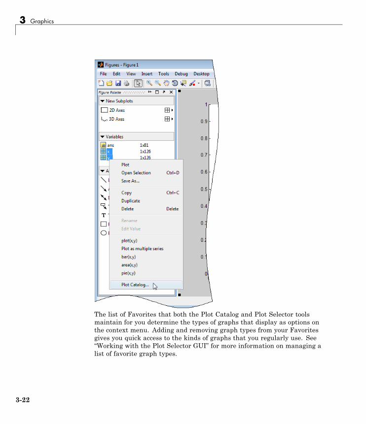
• In the Figure Palette component of the Plotting Tools, right-click a selectedvariable and choose Plot Catalog from the context menu
The following illustration of the Figure Palette tool shows two selectednumeric variables and the right-click context menu displayed. The PlotCatalog option is the bottom item on the menu.
3-21
3 Graphics
The list of Favorites that both the Plot Catalog and Plot Selector toolsmaintain for you determine the types of graphs that display as options onthe context menu. Adding and removing graph types from your Favoritesgives you quick access to the kinds of graphs that you regularly use. See“Working with the Plot Selector GUI” for more information on managing alist of favorite graph types.
3-22
Overview of Plotting
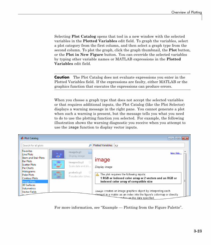
Selecting Plot Catalog opens that tool in a new window with the selectedvariables in the Plotted Variables edit field. To graph the variables, selecta plot category from the first column, and then select a graph type from thesecond column. To plot the graph, click the graph thumbnail, the Plot button,or the Plot in New Figure button. You can override the selected variablesby typing other variable names or MATLAB expressions in the PlottedVariables edit field.
Caution The Plot Catalog does not evaluate expressions you enter in thePlotted Variables field. If the expressions are faulty, either MATLAB or thegraphics function that executes the expressions can produce errors.
When you choose a graph type that does not accept the selected variablesor that requires additional inputs, the Plot Catalog (like the Plot Selector)displays a warning message in the right pane. You cannot generate a plotwhen such a warning is present, but the message tells you what you needto do to use the plotting function you selected. For example, the followingillustration shows the warning diagnostic you receive when you attempt touse the image function to display vector inputs.
For more information, see “Example — Plotting from the Figure Palette”.
3-23
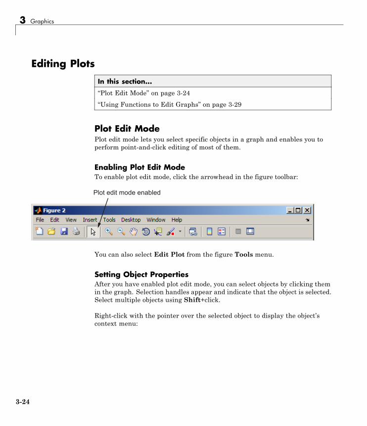
3 Graphics
Editing Plots
In this section...
“Plot Edit Mode” on page 3-24
“Using Functions to Edit Graphs” on page 3-29
Plot Edit ModePlot edit mode lets you select specific objects in a graph and enables you toperform point-and-click editing of most of them.
Enabling Plot Edit ModeTo enable plot edit mode, click the arrowhead in the figure toolbar:
&�����������������#���
You can also select Edit Plot from the figure Tools menu.
Setting Object PropertiesAfter you have enabled plot edit mode, you can select objects by clicking themin the graph. Selection handles appear and indicate that the object is selected.Select multiple objects using Shift+click.
Right-click with the pointer over the selected object to display the object’scontext menu:
3-24
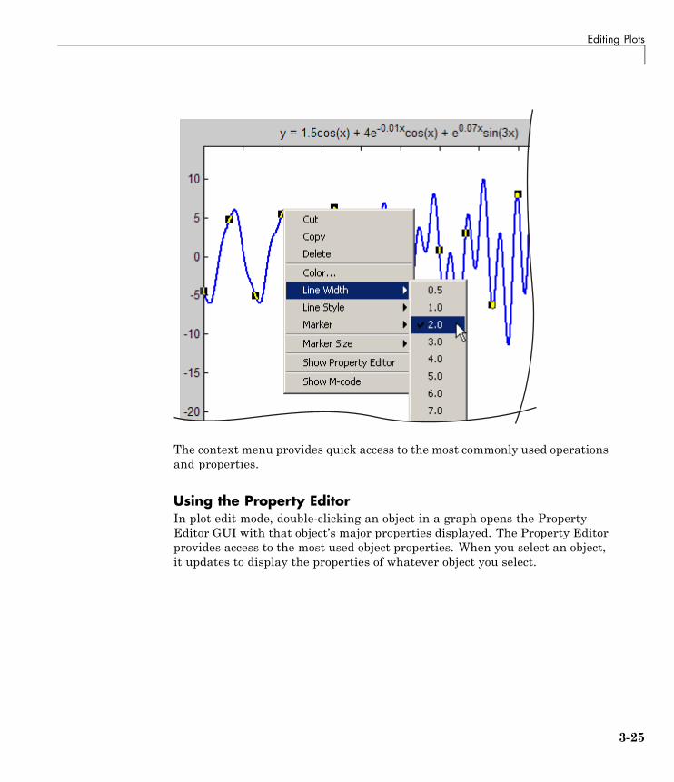
Editing Plots
The context menu provides quick access to the most commonly used operationsand properties.
Using the Property EditorIn plot edit mode, double-clicking an object in a graph opens the PropertyEditor GUI with that object’s major properties displayed. The Property Editorprovides access to the most used object properties. When you select an object,it updates to display the properties of whatever object you select.
3-25

3 Graphics
$��%���������� �&������ �'�������
Accessing Properties with the Property InspectorThe Property Inspector is a tool that enables you to access most HandleGraphics properties and other MATLAB objects. If you do not find theproperty you want to set in the Property Editor, click the More Propertiesbutton to display the Property Inspector. You can also use the inspectcommand to start the Property Inspector. For example, to inspect theproperties of the current axes, type
inspect(gca)
3-26
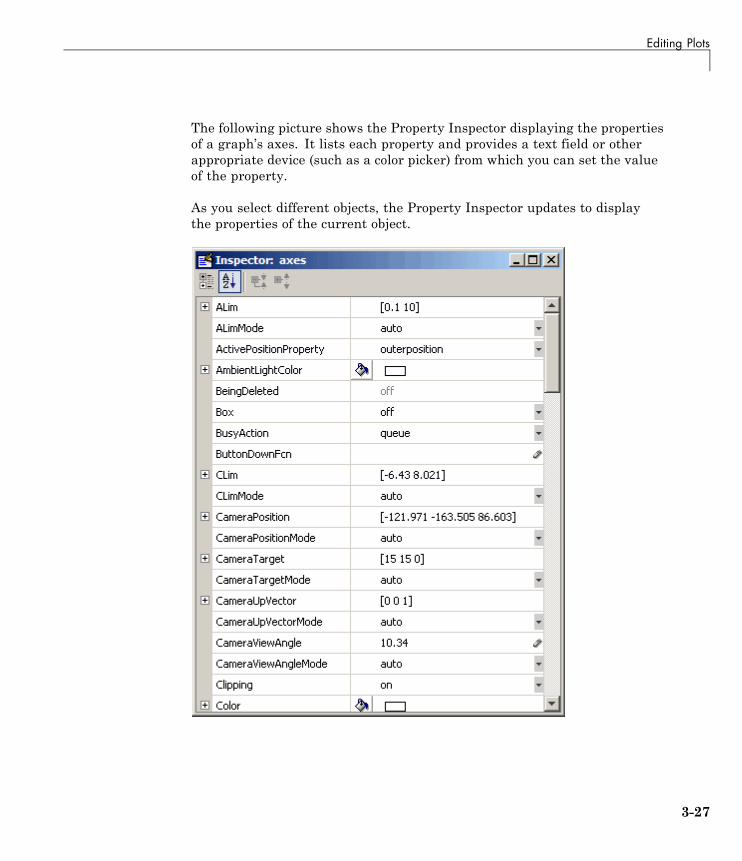
Editing Plots
The following picture shows the Property Inspector displaying the propertiesof a graph’s axes. It lists each property and provides a text field or otherappropriate device (such as a color picker) from which you can set the valueof the property.
As you select different objects, the Property Inspector updates to displaythe properties of the current object.
3-27
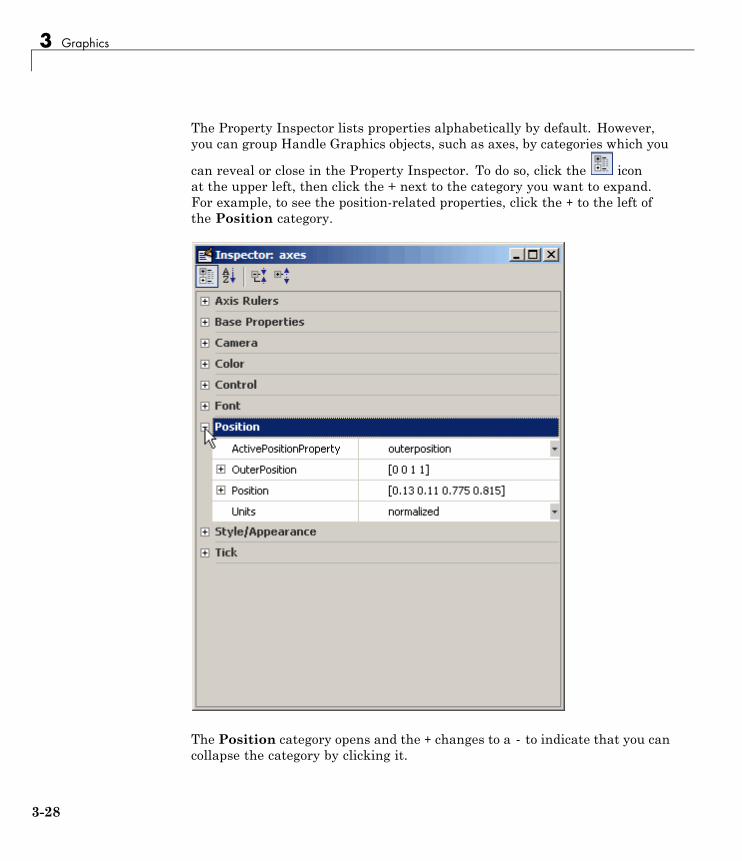
3 Graphics
The Property Inspector lists properties alphabetically by default. However,you can group Handle Graphics objects, such as axes, by categories which you
can reveal or close in the Property Inspector. To do so, click the iconat the upper left, then click the + next to the category you want to expand.For example, to see the position-related properties, click the + to the left ofthe Position category.
The Position category opens and the + changes to a - to indicate that you cancollapse the category by clicking it.
3-28
Editing Plots
Using Functions to Edit GraphsIf you prefer to work from the MATLAB command line, or if you are creatinga MATLAB program file, you can use MATLAB commands to edit the graphsyou create. You can use the set and get commands to change the properties ofthe objects in a graph. For more information about using graphics commands,see “Understanding Handle Graphics Objects” on page 3-85.
3-29
3 Graphics
Some Ways to Use Plotting Tools
In this section...
“Plotting Two Variables with Plotting Tools” on page 3-30
“Changing the Appearance of Lines and Markers” on page 3-33
“Adding More Data to the Graph” on page 3-34
“Changing the Type of Graph” on page 3-37
“Modifying the Graph Data Source” on page 3-39
Plotting Two Variables with Plotting ToolsSuppose you want to graph the function y = x3 over the x domain -1 to 1. Thefirst step is to generate the data to plot.
It is simple to evaluate a function like this because the MATLAB software candistribute arithmetic operations over all elements of a multivalued variable.
For example, the following statement creates a variable x that contains valuesranging from -1 to 1 in increments of 0.1 (you could also use the linspacefunction to generate data for x). The second statement raises each value inx to the third power and stores these values in y:
x = -1:.1:1; % Define the range of xy = x.^3; % Raise each element in x to the third power
Now that you have generated some data, you can plot it using the MATLABplotting tools. To start the plotting tools, type
plottools
A figure displays with plotting tools attached.
3-30
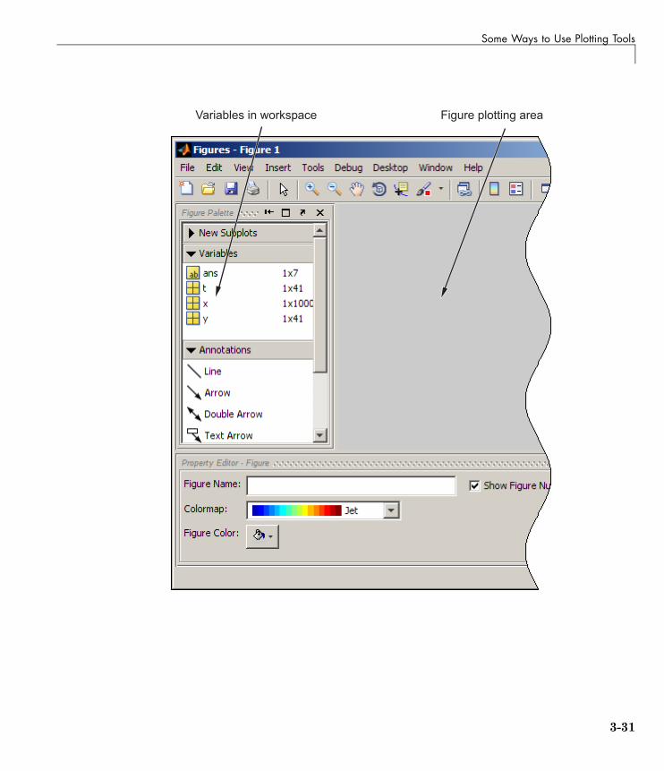
Some Ways to Use Plotting Tools
�����#����������%���� !� ����������� �����
3-31
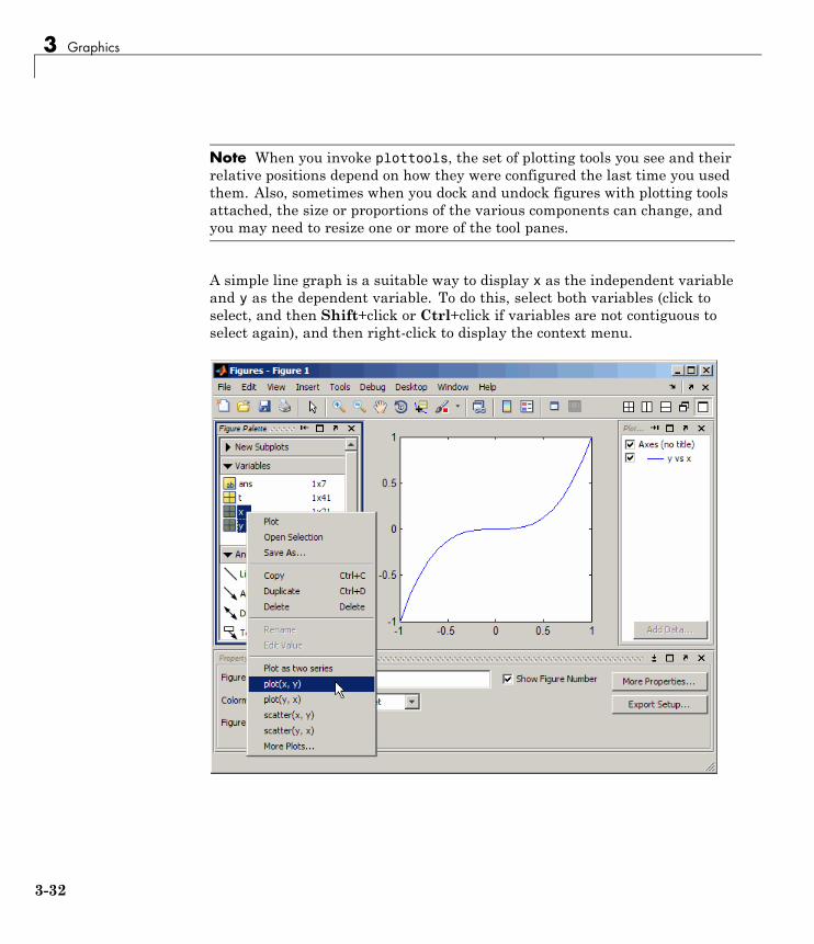
3 Graphics
Note When you invoke plottools, the set of plotting tools you see and theirrelative positions depend on how they were configured the last time you usedthem. Also, sometimes when you dock and undock figures with plotting toolsattached, the size or proportions of the various components can change, andyou may need to resize one or more of the tool panes.
A simple line graph is a suitable way to display x as the independent variableand y as the dependent variable. To do this, select both variables (click toselect, and then Shift+click or Ctrl+click if variables are not contiguous toselect again), and then right-click to display the context menu.
3-32
Some Ways to Use Plotting Tools
Select plot(x, y) from the menu. The line graph plots in the figure area. Theblack squares indicate that the line is selected and you can edit its propertieswith the Property Editor.
Changing the Appearance of Lines and MarkersNext, change the line properties so that the graph displays only the datapoint. Use the Property Editor to set following properties:
• Line to no line
• Marker to o (circle)
• Marker size to 4.0
• Marker fill color to red
3-33
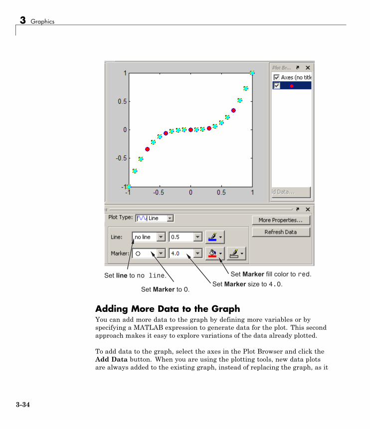
3 Graphics
(�������������������
(��������������
(������������������������
(������������������� �
Adding More Data to the GraphYou can add more data to the graph by defining more variables or byspecifying a MATLAB expression to generate data for the plot. This secondapproach makes it easy to explore variations of the data already plotted.
To add data to the graph, select the axes in the Plot Browser and click theAdd Data button. When you are using the plotting tools, new data plotsare always added to the existing graph, instead of replacing the graph, as it
3-34

Some Ways to Use Plotting Tools
would if you issued repeated plotting commands. Thus, the plotting toolsare in a hold on state.
To add data using the Plot Browser:
1 Click the Edit Plot tool .
2 Select the axes to which you wish to add data;handles appear around it.
3 Click the Add Data button in the Plot Browser;the Add Data to Axes dialog box opens.
4 Select a plot type from the Plot Type drop-down menu.
5 Select a variable or type an expression for X Data Source.
6 Select a variable or type an expression for Y Data Source.
7 Click OK;a plot of the data you specified is added to the axes.
3-35
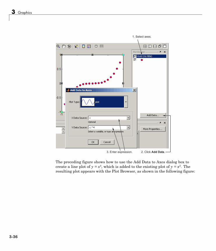
3 Graphics
)��(������"���
*��$��%���� ����+���������"���������
The preceding figure shows how to use the Add Data to Axes dialog box tocreate a line plot of y = x4, which is added to the existing plot of y = x3. Theresulting plot appears with the Plot Browser, as shown in the following figure:
3-36
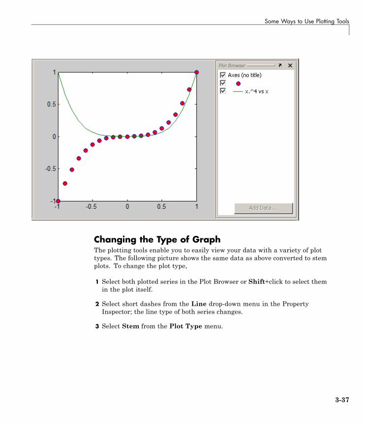
Some Ways to Use Plotting Tools
Changing the Type of GraphThe plotting tools enable you to easily view your data with a variety of plottypes. The following picture shows the same data as above converted to stemplots. To change the plot type,
1 Select both plotted series in the Plot Browser or Shift+click to select themin the plot itself.
2 Select short dashes from the Line drop-down menu in the PropertyInspector; the line type of both series changes.
3 Select Stem from the Plot Type menu.
3-37
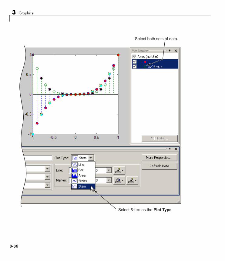
3 Graphics
(�����#����������������
(��������������������������
3-38
Some Ways to Use Plotting Tools
Modifying the Graph Data SourceYou can link graph data to variables in your workspace. When you changethe values contained in the variables, you can then update the graph to usethe new data without having to create a new graph. (See also the refreshfunction.)
1 Define 50 points between -3π and 3π and compute their sines and cosines:
x = linspace(-3*pi,3*pi,50);ys = sin(x);yc = cos(x);
2 Using the plotting tools, create a graph of ys = sin(x):
figureplottools
3 In the Figure Palette, alternate-click to select x and ys in the Variablepane.
4 Right-click either selected variable and choose plot(x, ys) from the contextmenu, as the following figure shows.
3-39
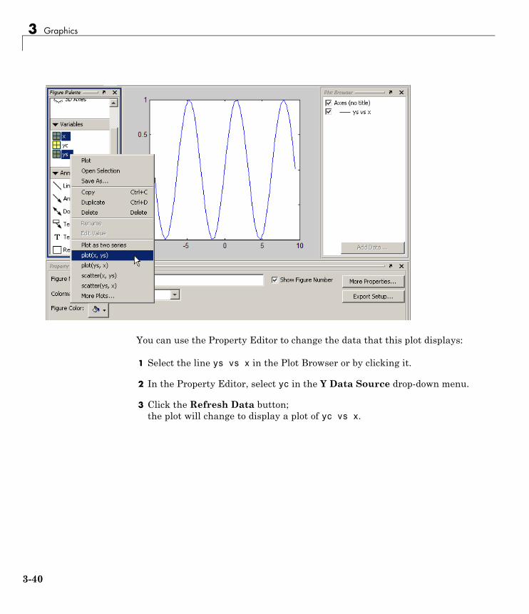
3 Graphics
You can use the Property Editor to change the data that this plot displays:
1 Select the line ys vs x in the Plot Browser or by clicking it.
2 In the Property Editor, select yc in the Y Data Source drop-down menu.
3 Click the Refresh Data button;the plot will change to display a plot of yc vs x.
3-40

Some Ways to Use Plotting Tools
Providing New Values for the Data SourceData values that define the graph are copies of variables in the baseworkspace (for example, x and y) to the XData and YData properties of theplot object (for example, a lineseries). Therefore, in addition to being able tochoose new data sources, you can assign new values to workspace variablesin the Command Window and click the Refresh Data button to update agraph to use the new data.
x = linspace(-pi,pi,50); % Define 50 points between - andy = sin(x);area(x,y) % Make an area plot of x and y
3-41
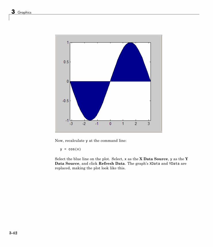
3 Graphics
Now, recalculate y at the command line:
y = cos(x)
Select the blue line on the plot. Select, x as the X Data Source, y as the YData Source, and click Refresh Data. The graph’s XData and YData arereplaced, making the plot look like this.
3-42
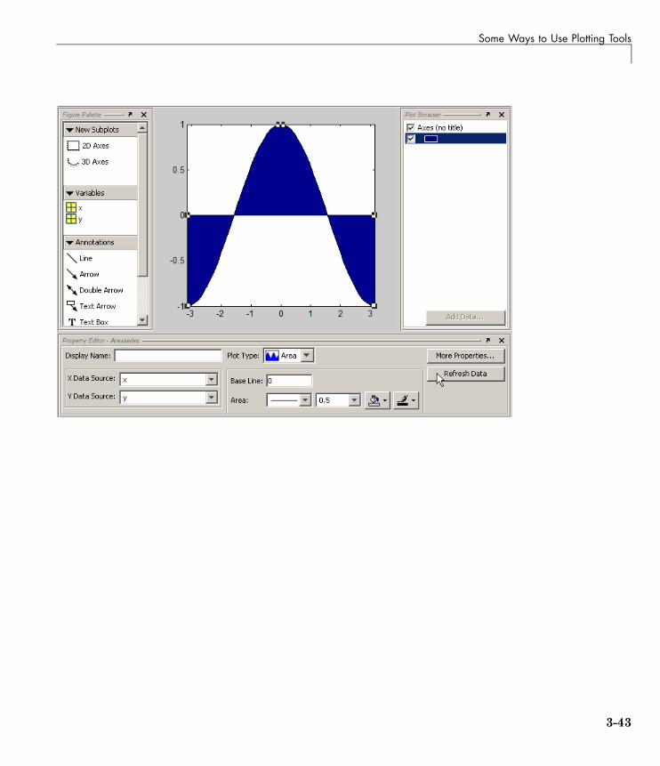
Some Ways to Use Plotting Tools
3-43

3 Graphics
Preparing Graphs for Presentation
In this section...
“Annotating Graphs for Presentation” on page 3-44
“Printing the Graph” on page 3-49
“Exporting the Graph” on page 3-53
Annotating Graphs for PresentationSuppose you plot the following data and want to create a graph that presentscertain information about the data:
x = -10:.005:40;y = [1.5*cos(x)+4*exp(-.01*x).*cos(x)+exp(.07*x).*sin(3*x)];plot(x,y)
This figure shows the graph created by the previous code.
3-44
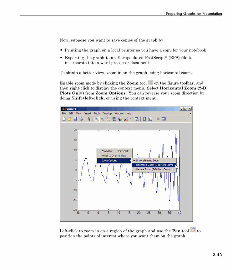
Preparing Graphs for Presentation
Now, suppose you want to save copies of the graph by
• Printing the graph on a local printer so you have a copy for your notebook
• Exporting the graph to an Encapsulated PostScript® (EPS) file toincorporate into a word processor document
To obtain a better view, zoom in on the graph using horizontal zoom.
Enable zoom mode by clicking the Zoom tool on the figure toolbar, andthen right-click to display the context menu. Select Horizontal Zoom (2-DPlots Only) from Zoom Options. You can reverse your zoom direction bydoing Shift+left-click, or using the context menu.
Left-click to zoom in on a region of the graph and use the Pan tool toposition the points of interest where you want them on the graph.
3-45
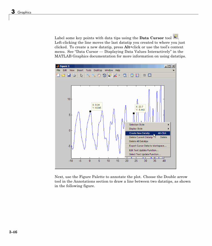
3 Graphics
Label some key points with data tips using the Data Cursor tool .Left-clicking the line moves the last datatip you created to where you justclicked. To create a new datatip, press Alt+click or use the tool’s contextmenu. See “Data Cursor — Displaying Data Values Interactively” in theMATLAB Graphics documentation for more information on using datatips.
Next, use the Figure Palette to annotate the plot. Choose the Double arrowtool in the Annotations section to draw a line between two datatips, as shownin the following figure.
3-46
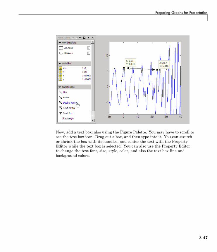
Preparing Graphs for Presentation
Now, add a text box, also using the Figure Palette. You may have to scroll tosee the text box icon. Drag out a box, and then type into it. You can stretchor shrink the box with its handles, and center the text with the PropertyEditor while the text box is selected. You can also use the Property Editorto change the text font, size, style, color, and also the text box line andbackground colors.
3-47
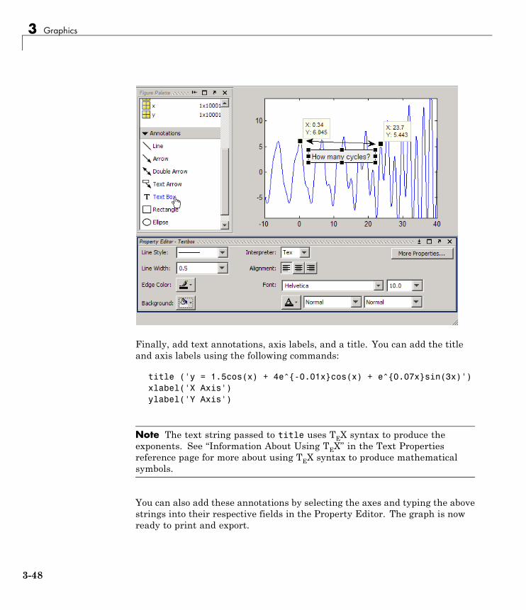
3 Graphics
Finally, add text annotations, axis labels, and a title. You can add the titleand axis labels using the following commands:
title ('y = 1.5cos(x) + 4e^{-0.01x}cos(x) + e^{0.07x}sin(3x)')xlabel('X Axis')ylabel('Y Axis')
Note The text string passed to title uses TEX syntax to produce theexponents. See “Information About Using TEX” in the Text Propertiesreference page for more about using TEX syntax to produce mathematicalsymbols.
You can also add these annotations by selecting the axes and typing the abovestrings into their respective fields in the Property Editor. The graph is nowready to print and export.
3-48
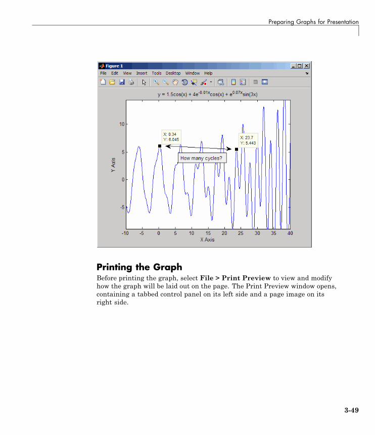
Preparing Graphs for Presentation
Printing the GraphBefore printing the graph, select File > Print Preview to view and modifyhow the graph will be laid out on the page. The Print Preview window opens,containing a tabbed control panel on its left side and a page image on itsright side.
3-49
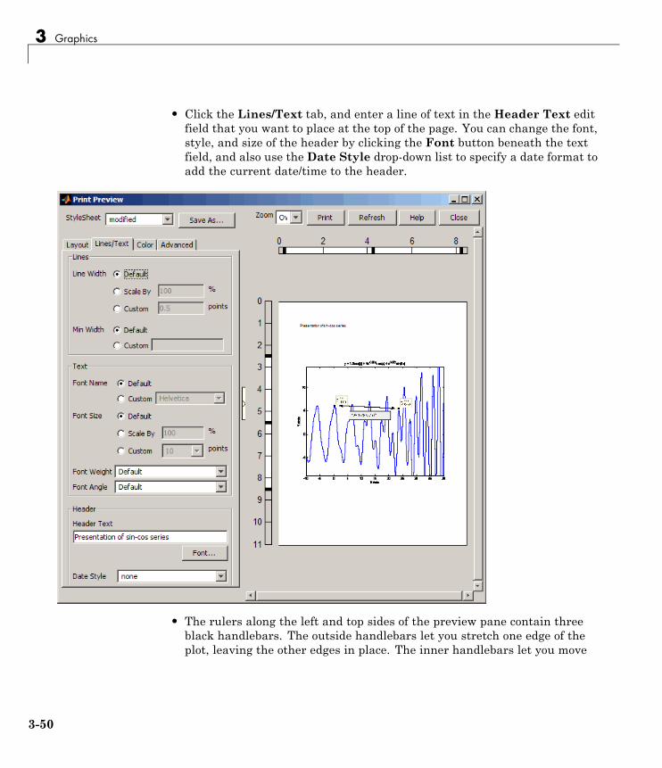
3 Graphics
• Click the Lines/Text tab, and enter a line of text in the Header Text editfield that you want to place at the top of the page. You can change the font,style, and size of the header by clicking the Font button beneath the textfield, and also use the Date Style drop-down list to specify a date format toadd the current date/time to the header.
• The rulers along the left and top sides of the preview pane contain threeblack handlebars. The outside handlebars let you stretch one edge of theplot, leaving the other edges in place. The inner handlebars let you move
3-50
Preparing Graphs for Presentation
the plot up and down or left and right without stretching it. Using themdoes not affect the figure itself, only the printed version of it.
• You can also change the size and position of the plot on the page using thebuttons and edit boxes on the Layout tab. You can revert to the originalconfiguration by clicking the Auto (Actual Size, Centered) option button,and correct stretching and shrinking by clicking Fix Aspect Ratio. Thefollowing picture shows the Layout tab in Auto configuration.
3-51
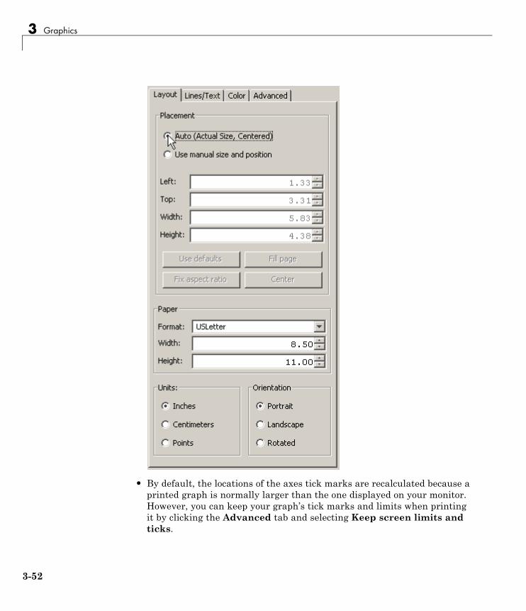
3 Graphics
• By default, the locations of the axes tick marks are recalculated because aprinted graph is normally larger than the one displayed on your monitor.However, you can keep your graph’s tick marks and limits when printingit by clicking the Advanced tab and selecting Keep screen limits andticks.
3-52
Preparing Graphs for Presentation
• When you are ready to print your plot, click Print in the right pane. Youcan also click Close to accept the settings and dismiss the dialog box.Later, you can print the figure as you previewed it using Print on thefigure’s File menu. Both methods will open a standard Print dialog box,and will produce the same printed results.
Note There is no way to cancel a print preview; any changes you makewill take effect if you print the figure. If you want to revert to a defaultpage layout, you can generally accomplish this by selecting either the UseDefaults button or the Auto (Actual Size, Centered) option button on theLayout tab, although this will not affect every setting you can make.
The Print Preview dialog box provides many other options for controlling howprinted graphs look. Click its Help button for more information.
Exporting the GraphExporting a graph is the process of creating a standard graphics file formatof the graph (such as EPS or TIFF), which you can then import into otherapplications like word processors, drawing packages, etc.
This example exports the graph as an EPS file with the followingrequirements:
• The size of the picture when imported into the word processor documentshould be 4 inches wide and 3 inches high.
• All the text in the figure should have a size of 8 points.
Specifying the Size of the GraphTo set the size, use the Export Setup dialog box (select Export Setup fromthe figure File menu). Then select 4 from the Width list and 3 from theHeight list.
3-53
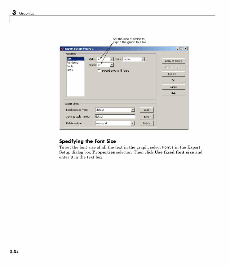
3 Graphics
(��������������������"�������� ��������������
Specifying the Font SizeTo set the font size of all the text in the graph, select Fonts in the ExportSetup dialog box Properties selector. Then click Use fixed font size andenter 8 in the text box.
3-54
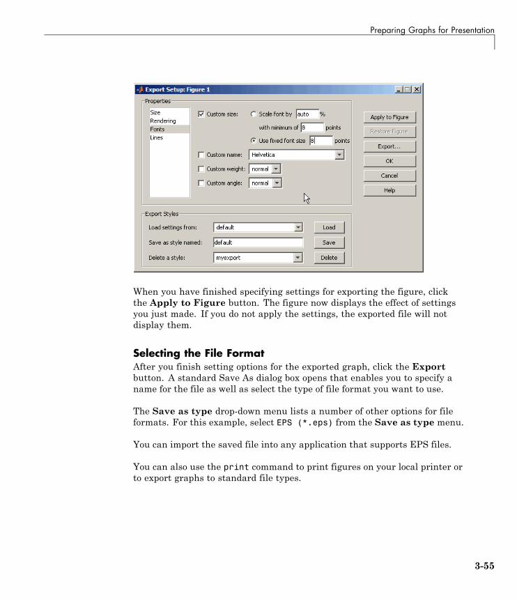
Preparing Graphs for Presentation
When you have finished specifying settings for exporting the figure, clickthe Apply to Figure button. The figure now displays the effect of settingsyou just made. If you do not apply the settings, the exported file will notdisplay them.
Selecting the File FormatAfter you finish setting options for the exported graph, click the Exportbutton. A standard Save As dialog box opens that enables you to specify aname for the file as well as select the type of file format you want to use.
The Save as type drop-down menu lists a number of other options for fileformats. For this example, select EPS (*.eps) from the Save as type menu.
You can import the saved file into any application that supports EPS files.
You can also use the print command to print figures on your local printer orto export graphs to standard file types.
3-55

3 Graphics
For More Information See the print command reference page and “Printingand Exporting” in the MATLAB Graphics documentation or select Printingand Exporting from the figure Help menu.
3-56
Using Basic Plotting Functions
Using Basic Plotting Functions
In this section...
“Creating a Plot” on page 3-57
“Plotting Multiple Data Sets in One Graph” on page 3-58
“Specifying Line Styles and Colors” on page 3-59
“Plotting Lines and Markers” on page 3-60
“Graphing Imaginary and Complex Data” on page 3-62
“Adding Plots to an Existing Graph” on page 3-63
“Figure Windows” on page 3-64
“Displaying Multiple Plots in One Figure” on page 3-65
“Controlling the Axes” on page 3-67
“Adding Axis Labels and Titles” on page 3-68
“Saving Figures” on page 3-69
Creating a PlotThe plot function has different forms, depending on the input arguments. Ify is a vector, plot(y) produces a piecewise linear graph of the elements of yversus the index of the elements of y. If you specify two vectors as arguments,plot(x,y) produces a graph of y versus x.
For example, these statements use the colon operator to create a vector ofx values ranging from 0 to 2π, compute the sine of these values, and plotthe result:
x = 0:pi/100:2*pi;y = sin(x);plot(x,y)
Now label the axes and add a title. The characters \pi create the symbol π.See “text strings” in the MATLAB Reference documentation for more symbols:
xlabel('x = 0:2\pi')ylabel('Sine of x')
3-57
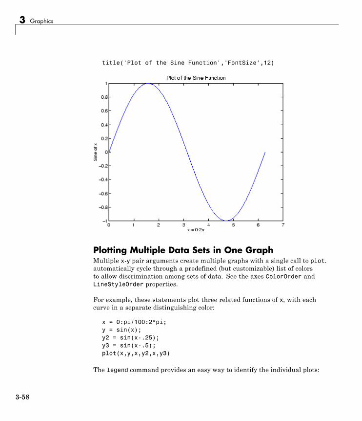
3 Graphics
title('Plot of the Sine Function','FontSize',12)
Plotting Multiple Data Sets in One GraphMultiple x-y pair arguments create multiple graphs with a single call to plot.automatically cycle through a predefined (but customizable) list of colorsto allow discrimination among sets of data. See the axes ColorOrder andLineStyleOrder properties.
For example, these statements plot three related functions of x, with eachcurve in a separate distinguishing color:
x = 0:pi/100:2*pi;y = sin(x);y2 = sin(x-.25);y3 = sin(x-.5);plot(x,y,x,y2,x,y3)
The legend command provides an easy way to identify the individual plots:
3-58
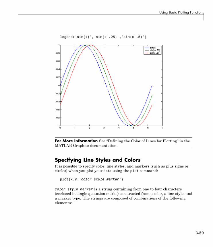
Using Basic Plotting Functions
legend('sin(x)','sin(x-.25)','sin(x-.5)')
For More Information See “Defining the Color of Lines for Plotting” in theMATLAB Graphics documentation.
Specifying Line Styles and ColorsIt is possible to specify color, line styles, and markers (such as plus signs orcircles) when you plot your data using the plot command:
plot(x,y,'color_style_marker')
color_style_marker is a string containing from one to four characters(enclosed in single quotation marks) constructed from a color, a line style, anda marker type. The strings are composed of combinations of the followingelements:
3-59
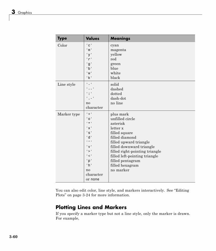
3 Graphics
Type Values Meanings
Color 'c''m''y''r''g''b''w''k'
cyanmagentayellowredgreenbluewhiteblack
Line style '-''--'':''.-'nocharacter
soliddasheddotteddash-dotno line
Marker type '+''o''*''x''s''d''^''v''>''<''p''h'nocharacteror none
plus markunfilled circleasteriskletter xfilled squarefilled diamondfilled upward trianglefilled downward trianglefilled right-pointing trianglefilled left-pointing trianglefilled pentagramfilled hexagramno marker
You can also edit color, line style, and markers interactively. See “EditingPlots” on page 3-24 for more information.
Plotting Lines and MarkersIf you specify a marker type but not a line style, only the marker is drawn.For example,
3-60
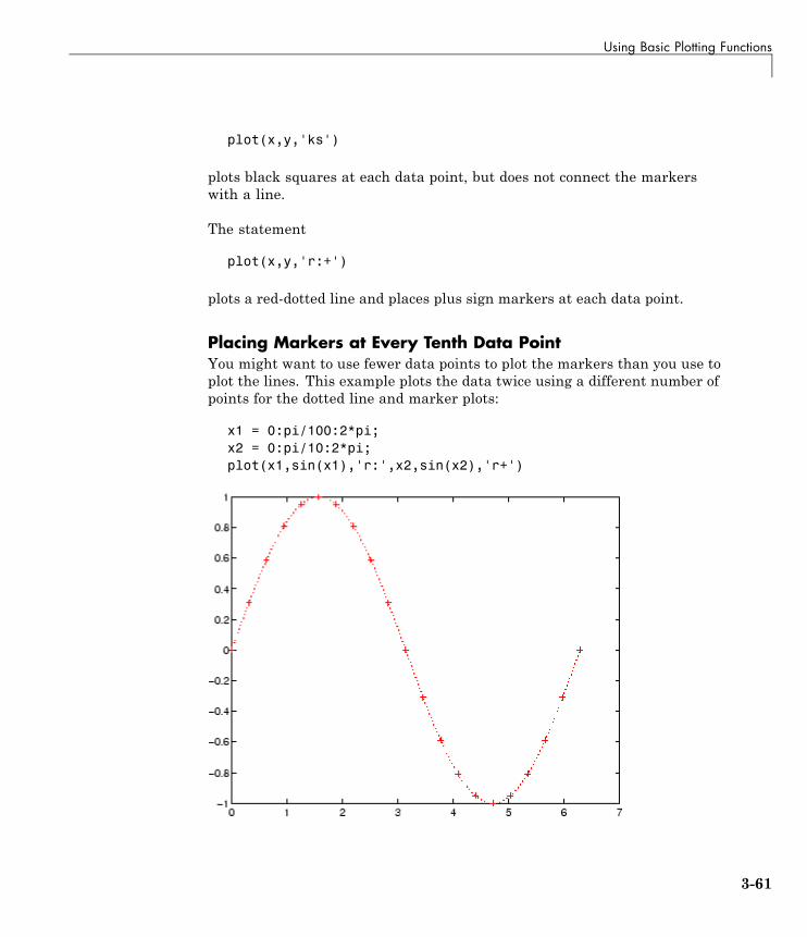
Using Basic Plotting Functions
plot(x,y,'ks')
plots black squares at each data point, but does not connect the markerswith a line.
The statement
plot(x,y,'r:+')
plots a red-dotted line and places plus sign markers at each data point.
Placing Markers at Every Tenth Data PointYou might want to use fewer data points to plot the markers than you use toplot the lines. This example plots the data twice using a different number ofpoints for the dotted line and marker plots:
x1 = 0:pi/100:2*pi;x2 = 0:pi/10:2*pi;plot(x1,sin(x1),'r:',x2,sin(x2),'r+')
3-61
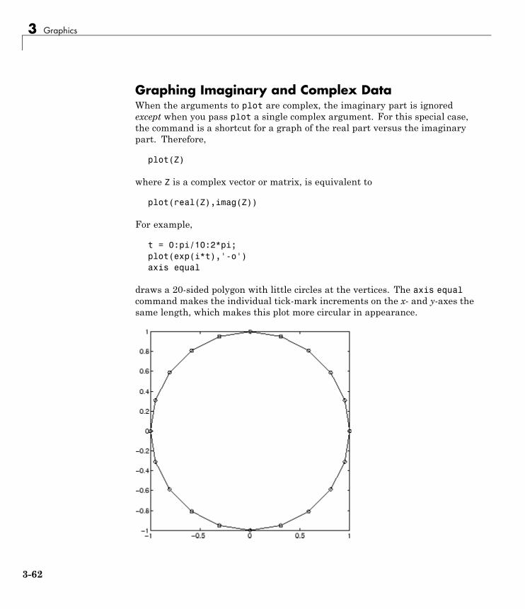
3 Graphics
Graphing Imaginary and Complex DataWhen the arguments to plot are complex, the imaginary part is ignoredexcept when you pass plot a single complex argument. For this special case,the command is a shortcut for a graph of the real part versus the imaginarypart. Therefore,
plot(Z)
where Z is a complex vector or matrix, is equivalent to
plot(real(Z),imag(Z))
For example,
t = 0:pi/10:2*pi;plot(exp(i*t),'-o')axis equal
draws a 20-sided polygon with little circles at the vertices. The axis equalcommand makes the individual tick-mark increments on the x- and y-axes thesame length, which makes this plot more circular in appearance.
3-62
Using Basic Plotting Functions
Adding Plots to an Existing GraphThe MATLAB hold command enables you to add plots to an existing graph.When you type
hold on
Now MATLAB does not replace the existing graph when you issue anotherplotting command; it adds the new data to the current graph, rescaling theaxes if necessary.
For example, these statements first create a contour plot of the peaksfunction, then superimpose a pseudocolor plot of the same function:
[x,y,z] = peaks;pcolor(x,y,z)shading interphold oncontour(x,y,z,20,'k')hold off
The hold on command combines the pcolor plot with the contour plot inone figure.
3-63
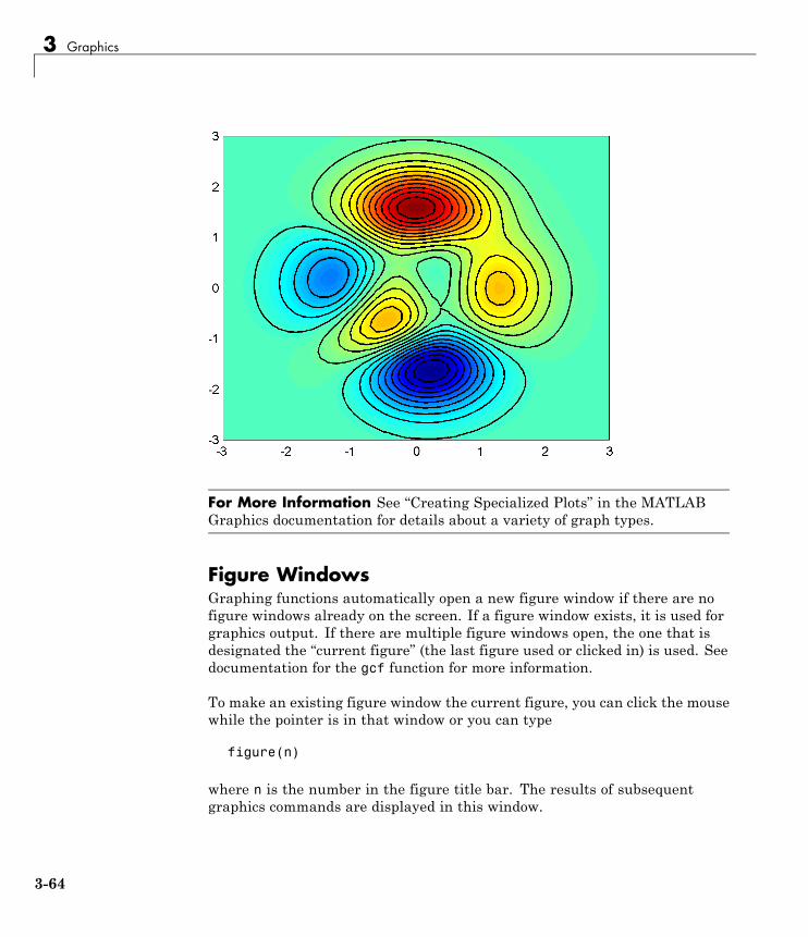
3 Graphics
For More Information See “Creating Specialized Plots” in the MATLABGraphics documentation for details about a variety of graph types.
Figure WindowsGraphing functions automatically open a new figure window if there are nofigure windows already on the screen. If a figure window exists, it is used forgraphics output. If there are multiple figure windows open, the one that isdesignated the “current figure” (the last figure used or clicked in) is used. Seedocumentation for the gcf function for more information.
To make an existing figure window the current figure, you can click the mousewhile the pointer is in that window or you can type
figure(n)
where n is the number in the figure title bar. The results of subsequentgraphics commands are displayed in this window.
3-64
Using Basic Plotting Functions
To open a new figure window and make it the current figure, type
figure
Clearing the Figure for a New PlotWhen a figure already exists, most plotting commands clear the axes and usethis figure to create the new plot. However, these commands do not resetfigure properties, such as the background color or the colormap. If you haveset any figure properties in the previous plot, you might want to use the clfcommand with the reset option,
clf reset
before creating your new plot to restore the figure’s properties to theirdefaults.
For More Information See “Using Figure Properties” and “GraphicsWindows — the Figure” in the MATLAB Graphics documentation for detailsabout figures.
Displaying Multiple Plots in One FigureThe subplot command enables you to display multiple plots in the samewindow or print them on the same piece of paper. Typing
subplot(m,n,p)
partitions the figure window into an m-by-n matrix of small subplots andselects the pth subplot for the current plot. The plots are numbered along thefirst row of the figure window, then the second row, and so on. For example,these statements plot data in four different subregions of the figure window:
t = 0:pi/10:2*pi;[X,Y,Z] = cylinder(4*cos(t));subplot(2,2,1); mesh(X)subplot(2,2,2); mesh(Y)subplot(2,2,3); mesh(Z)subplot(2,2,4); mesh(X,Y,Z)
3-65

3 Graphics
You can add subplots to GUIs as well as to figures. For details about creatingsubplots in a GUIDE-generated GUI, see “Creating Subplots” in the MATLABCreating Graphical User Interfaces documentation.
3-66
Using Basic Plotting Functions
Controlling the AxesThe axis command provides a number of options for setting the scaling,orientation, and aspect ratio of graphs. You can also set these optionsinteractively. See “Editing Plots” on page 3-24 for more information.
Setting Axis LimitsBy default, MATLAB finds the maxima and minima of the data and choosesthe axis limits to span this range. The axis command enables you to specifyyour own limits:
axis([xmin xmax ymin ymax])
or for three-dimensional graphs,
axis([xmin xmax ymin ymax zmin zmax])
Use the command
axis auto
to enable automatic limit selection again.
Setting the Axis Aspect RatioThe axis command also enables you to specify a number of predefined modes.For example,
axis square
makes the x-axis and y-axis the same length.
axis equal
makes the individual tick mark increments on the x-axes and y-axes the samelength. This means
plot(exp(i*[0:pi/10:2*pi]))
followed by either axis square or axis equal turns the oval into a propercircle:
axis auto normal
3-67
3 Graphics
returns the axis scaling to its default automatic mode.
Setting Axis VisibilityYou can use the axis command to make the axis visible or invisible.
axis on
makes the axes visible. This is the default.
axis off
makes the axes invisible.
Setting Grid LinesThe grid command toggles grid lines on and off. The statement
grid on
turns the grid lines on, and
grid off
turns them back off again.
For More Information See the axis and axes reference pages and “UsingAxes Properties” in the MATLAB Graphics documentation.
Adding Axis Labels and TitlesThe xlabel, ylabel, and zlabel commands add x-, y-, and z-axis labels. Thetitle command adds a title at the top of the figure and the text functioninserts text anywhere in the figure.
You can produce mathematical symbols using LaTeX notation in the textstring, as the following example illustrates:
t = -pi:pi/100:pi;y = sin(t);plot(t,y)
3-68
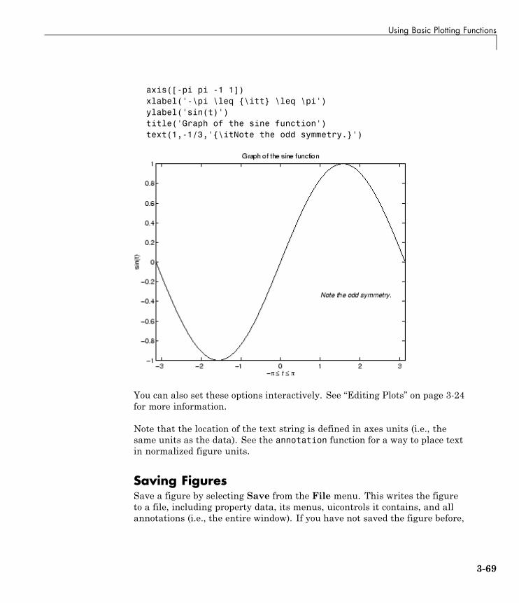
Using Basic Plotting Functions
axis([-pi pi -1 1])xlabel('-\pi \leq {\itt} \leq \pi')ylabel('sin(t)')title('Graph of the sine function')text(1,-1/3,'{\itNote the odd symmetry.}')
You can also set these options interactively. See “Editing Plots” on page 3-24for more information.
Note that the location of the text string is defined in axes units (i.e., thesame units as the data). See the annotation function for a way to place textin normalized figure units.
Saving FiguresSave a figure by selecting Save from the File menu. This writes the figureto a file, including property data, its menus, uicontrols it contains, and allannotations (i.e., the entire window). If you have not saved the figure before,
3-69

3 Graphics
the Save As dialog displays. This dialog provides options to save the figure asa FIG-file or export it to a graphics format.
If you have previously saved the figure, using Save again saves the figure“silently,” without displaying the Save As dialog.
To save a figure using a standard graphics format for use with otherapplications, such as TIFF or JPG, select Save As (or Export Setup, if youwant additional control) from the File menu.
Note Whenever you specify a format for saving a figure, that file format isused again the next time you save that figure or a new one. If you do not wantto save in the previously-used format, use Save As and be sure to set theSave as type drop-down menu to the kind of file you want to write.
You can also save from the command line—use the saveas command,including any options to save the figure in a different format. The morerestricted hgexport command, which saves figures to either bitmap ormetafile files, depending on the rendering method in effect, is also available.
See “Exporting the Graph” on page 3-53 for an example.
Saving Workspace DataYou can save the variables in your workspace by selecting Save WorkspaceAs from the figure File menu. You can reload saved data using the ImportData item in the figure File menu. MATLAB supports a variety of data fileformats, including MATLAB data files, which have a .mat extension.
Generating MATLAB Code to Recreate a FigureYou can generate MATLAB code that recreates a figure and the graph itcontains by selecting Generate code from the figure File menu. This optionis particularly useful if you have developed a graph using plotting tools andwant to create a similar graph using the same or different data.
3-70
Using Basic Plotting Functions
Saving Figures That Are Compatible with the Previous MATLABSoftware VersionCreate backward-compatible FIG-files by following these two steps:
1 Ensure that any plotting functions used to create the contents of the figureare called with the 'v6' argument, where applicable.
2 Use the '-v6' option with the hgsave command.
Note The v6 option enables users of Version 7.x of MATLAB to createFIG-files that previous versions can open. It is obsolete and will be removedin a future version of MATLAB. For more information, see “Plot Objects andBackward Compatibility” in the MATLAB Graphics documentation.
3-71

3 Graphics
Creating Mesh and Surface Plots
In this section...
“About Mesh and Surface Plots” on page 3-72
“Visualizing Functions of Two Variables” on page 3-72
About Mesh and Surface PlotsYou define a surface by the z-coordinates of points above a grid in the x-yplane, using straight lines to connect adjacent points. The mesh and surfplotting functions display surfaces in three dimensions. mesh produceswireframe surfaces that color only the lines connecting the defining points.surf displays both the connecting lines and the faces of the surface in color.
The figure colormap and figure properties determine how the surface iscolored.
Visualizing Functions of Two VariablesTo display a function of two variables, z = f (x,y),
1 Generate X and Y matrices consisting of repeated rows and columns,respectively, over the domain of the function.
2 Use X and Y to evaluate and graph the function.
The meshgrid function transforms the domain specified by a single vector ortwo vectors x and y into matrices X and Y for use in evaluating functions oftwo variables. The rows of X are copies of the vector x and the columns ofY are copies of the vector y.
Example — Graphing the sinc FunctionThis example evaluates and graphs the two-dimensional sinc function,sin(r)/r, between the x and y directions. R is the distance from the origin, whichis at the center of the matrix. Adding eps (a MATLAB command that returnsa small floating-point number) avoids the indeterminate 0/0 at the origin:
[X,Y] = meshgrid(-8:.5:8);
3-72
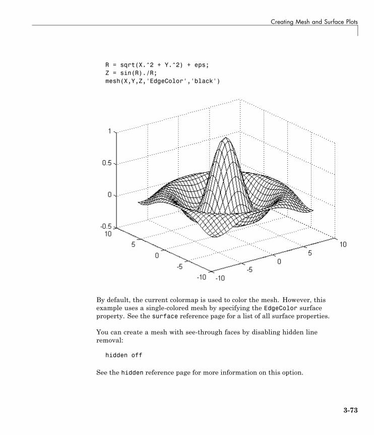
Creating Mesh and Surface Plots
R = sqrt(X.^2 + Y.^2) + eps;Z = sin(R)./R;mesh(X,Y,Z,'EdgeColor','black')
By default, the current colormap is used to color the mesh. However, thisexample uses a single-colored mesh by specifying the EdgeColor surfaceproperty. See the surface reference page for a list of all surface properties.
You can create a mesh with see-through faces by disabling hidden lineremoval:
hidden off
See the hidden reference page for more information on this option.
3-73

3 Graphics
Example — Colored Surface PlotsA surface plot is similar to a mesh plot except that the rectangular faces of thesurface are colored. The color of each face is determined by the values of Z andthe colormap (a colormap is an ordered list of colors). These statements graphthe sinc function as a surface plot, specify a colormap, and add a color bar toshow the mapping of data to color:
surf(X,Y,Z)colormap hsvcolorbar
See the colormap reference page for information on colormaps.
3-74
Creating Mesh and Surface Plots
For More Information See “Creating 3-D Graphs” in the MATLAB 3-DVisualization documentation for more information on surface plots.
Making Surfaces TransparentYou can make the faces of a surface transparent to a varying degree.Transparency (referred to as the alpha value) can be specified for the wholeobject or can be based on an alphamap, which behaves similarly to colormaps.For example,
surf(X,Y,Z)colormap hsvalpha(.4)
produces a surface with a face alpha value of 0.4. Alpha values range from 0(completely transparent) to 1 (not transparent).
3-75
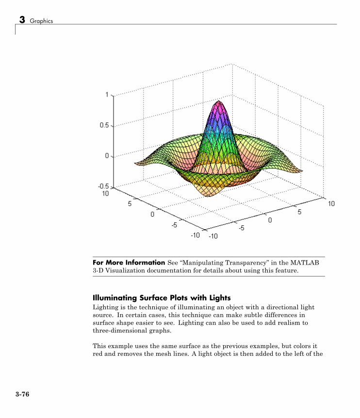
3 Graphics
For More Information See “Manipulating Transparency” in the MATLAB3-D Visualization documentation for details about using this feature.
Illuminating Surface Plots with LightsLighting is the technique of illuminating an object with a directional lightsource. In certain cases, this technique can make subtle differences insurface shape easier to see. Lighting can also be used to add realism tothree-dimensional graphs.
This example uses the same surface as the previous examples, but colors itred and removes the mesh lines. A light object is then added to the left of the
3-76
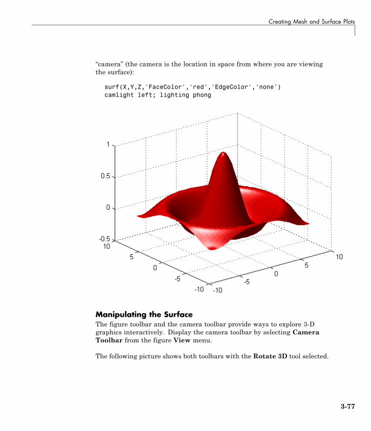
Creating Mesh and Surface Plots
“camera” (the camera is the location in space from where you are viewingthe surface):
surf(X,Y,Z,'FaceColor','red','EdgeColor','none')camlight left; lighting phong
Manipulating the SurfaceThe figure toolbar and the camera toolbar provide ways to explore 3-Dgraphics interactively. Display the camera toolbar by selecting CameraToolbar from the figure View menu.
The following picture shows both toolbars with the Rotate 3D tool selected.
3-77
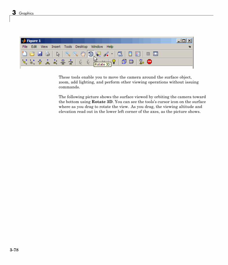
3 Graphics
These tools enable you to move the camera around the surface object,zoom, add lighting, and perform other viewing operations without issuingcommands.
The following picture shows the surface viewed by orbiting the camera towardthe bottom using Rotate 3D. You can see the tools’s cursor icon on the surfacewhere as you drag to rotate the view. As you drag, the viewing altitude andelevation read out in the lower left corner of the axes, as the picture shows.
3-78
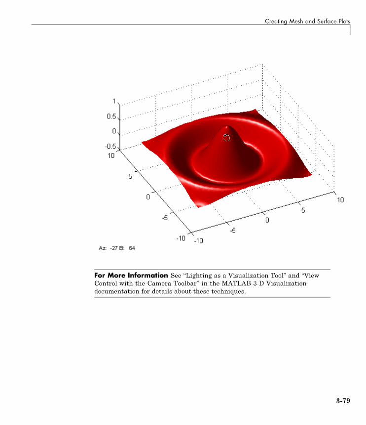
Creating Mesh and Surface Plots
For More Information See “Lighting as a Visualization Tool” and “ViewControl with the Camera Toolbar” in the MATLAB 3-D Visualizationdocumentation for details about these techniques.
3-79
3 Graphics
Plotting Image Data
In this section...
“About Plotting Image Data” on page 3-80
“Reading and Writing Images” on page 3-81
About Plotting Image DataTwo-dimensional arrays can be displayed as images, where the array elementsdetermine brightness or color of the images. For example, the statements
load durerwhosName Size Bytes Class
X 648x509 2638656 double arraycaption 2x28 112 char arraymap 128x3 3072 double array
load the file durer.mat, adding three variables to the workspace. The matrixX is a 648-by-509 matrix and map is a 128-by-3 matrix that is the colormap forthis image.
MAT-files, such as durer.mat, are binary files that can be created on oneplatform and later read by the MATLAB software on a different platform.
The elements of X are integers between 1 and 128, which serve as indicesinto the colormap, map. Then
image(X)colormap(map)axis image
reproduces Albrecht Dürer’s etching shown in “Matrices and Magic Squares”on page 2-2. A high-resolution scan of the magic square in the upper-rightcorner is available in another file. Type
load detail
3-80
Plotting Image Data
and then use the up arrow key on your keyboard to reexecute the image,colormap, and axis commands. The statement
colormap(hot)
adds some 21st century colorization to the 16th century etching. The functionhot generates a colormap containing shades of reds, oranges, and yellows.Typically, a given image matrix has a specific colormap associated with it.See the colormap reference page for a list of other predefined colormaps.
Reading and Writing ImagesYou can read standard image files (TIFF, JPEG, BMP, etc using the imreadfunction. The type of data returned by imread depends on the type of imageyou are reading.
You can write MATLAB data to a variety of standard image formats usingthe imwrite function. See the MATLAB reference pages for these functionsfor more information and examples.
For More Information See “Displaying Bit-Mapped Images” in the MATLABGraphics documentation for details about MATLAB image processingcapabilities.
3-81
3 Graphics
Printing Graphics
In this section...
“Overview of Printing” on page 3-82
“Printing from the File Menu” on page 3-82
“Exporting the Figure to a Graphics File” on page 3-83
“Using the Print Command” on page 3-83
Overview of PrintingYou can print a MATLAB figure directly on a printer connected to yourcomputer or you can export the figure to one of the standard graphics fileformats that MATLAB supports. There are two ways to print and exportfigures:
• Use the Print, Print Preview, or Export Setup GUI options under theFile menu; see “Preparing Graphs for Presentation” on page 3-44 for anexample.
• Use the print command to print or export the figure from the commandline.
The print command provides greater control over drivers and file formats.The Print Preview dialog box gives you greater control over figure size,proportions, placement, and page headers. You can sometimes noticedifferences in output as printed from a GUI and as printed from the commandline.
Printing from the File MenuThere are two menu options under the File menu that pertain to printing:
• The Print Preview option displays a dialog box that lets you lay out andstyle figures for printing while previewing the output page, and from whichyou can print the figure. It includes options that formerly were part ofthe Page Setup dialog box.
3-82
Printing Graphics
• The Print option displays a dialog box that lets you choose a printer, selectstandard printing options, and print the figure.
Use Print Preview to determine whether the printed output is what youwant. Click the Print Preview dialog box Help button to display informationon how to set up the page.
See “Printing the Graph” on page 3-49 for an example of printing fromthe Print Preview dialog. For details on printing from GUIs and from theCommand Window, see “Printing and Exporting” in the MATLAB Graphicsdocumentation.
Exporting the Figure to a Graphics FileThe Export Setup option in the File menu opens a GUI that enables youto set graphic characteristics, such as text size, font, and style, for figuresyou save as graphics files. The Export Setup GUI lets you define and applytemplates to customize and standardize output. After setup, you can exportthe figure to a number of standard graphics file formats such as EPS, PNG,and TIFF.
See “Exporting the Graph” on page 3-53 for an example of exporting a figureto a graphics file.
Using the Print CommandThe print command provides more flexibility in the type of output sent tothe printer and allows you to control printing from function and script files.The result can be sent directly to your default printer or stored in a specifiedoutput file. A wide variety of output formats, including TIFF, JPEG, andPostScript, is available.
For example, this statement saves the contents of the current figure windowas color Encapsulated Level 2 PostScript in the file called magicsquare.eps.It also includes a TIFF preview, which enables most word processors todisplay the picture.
print -depsc2 -tiff magicsquare.eps
3-83
3 Graphics
To save the same figure as a TIFF file with a resolution of 200 dpi, use thefollowing command:
print -dtiff -r200 magicsquare.tiff
If you type print on the command line
the current figure prints on your default printer.
For More Information See the print reference page and “Printing andExporting” in the MATLAB Graphics documentation for details aboutprinting.
3-84
Understanding Handle Graphics® Objects
Understanding Handle Graphics Objects
In this section...
“Using the Handle” on page 3-85
“Graphics Objects” on page 3-86
“Setting Object Properties” on page 3-88
“Specifying the Axes or Figure” on page 3-91
“Finding the Handles of Existing Objects” on page 3-93
Handle Graphics objects are MATLAB objects that implement graphing andvisualization functions. Each object created has a fixed set of properties. Youcan use these properties to control the behavior and appearance of your graph.
When you call a MATLAB plotting function, it creates the graph using variousgraphics objects, such as a figure window, axes, lines, text, and so on. You canquery the value of each property and set the values of most of them.
For example, the following statement creates a figure with a white backgroundcolor and without displaying the figure toolbar:
figure('Color','white','Toolbar','none')
Using the HandleWhenever MATLAB creates a graphics object, it assigns an identifier (called ahandle) to the object. You can use this handle to access the object’s propertieswith the set and get functions. For example, the following statements createa graph and return a handle to a lineseries object in h:
x = 1:10;y = x.^3;h = plot(x,y);
You can use the handle h to set the properties of the lineseries object. Forexample, you can set its Color property:
set(h,'Color','red')
You can also specify properties when you call the plotting function:
3-85
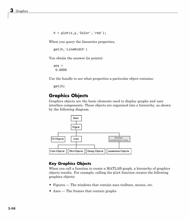
3 Graphics
h = plot(x,y,'Color','red');
When you query the lineseries properties,
get(h,'LineWidth')
You obtain the answer (in points):
ans =0.5000
Use the handle to see what properties a particular object contains:
get(h)
Graphics ObjectsGraphics objects are the basic elements used to display graphs and userinterface components. These objects are organized into a hierarchy, as shownby the following diagram.
Key Graphics ObjectsWhen you call a function to create a MATLAB graph, a hierarchy of graphicsobjects results. For example, calling the plot function creates the followinggraphics objects:
• Figures — The windows that contain axes toolbars, menus, etc.
• Axes — The frames that contain graphs
3-86
Understanding Handle Graphics® Objects
• Lineseries plot objects — Representations of data passed to the plotfunction.
• Text — Labels for axes tick marks and optional titles and annotations.
Different types of graphs use different objects to represent data. All dataobjects are contained in axes and all objects (except root) are contained infigures.
The root is an abstract object that primarily stores information about yourcomputer or MATLAB states. You cannot create an instance of the root object.The handle of the root object is always 0.
For More Information See “Handle Graphics Objects” in the MATLABGraphics documentation for details about graphics objects.
User interface objects are used to create graphical user interfaces (GUIs).These objects include components like push buttons, editable text boxes, andlist boxes.
For More Information See Chapter 6, “Creating Graphical User Interfaces”for details about user interface objects.
Creating ObjectsPlotting functions (like plot and surf) call the appropriate low-level functionto draw their respective graph. For information about an object’s properties,you can use the Handle Graphics Property Browser in the MATLAB onlineGraphics documentation.
Functions for Working with ObjectsThis table lists functions commonly used when working with objects.
3-87
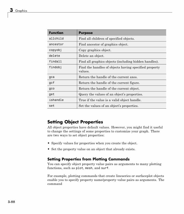
3 Graphics
Function Purpose
allchild Find all children of specified objects.
ancestor Find ancestor of graphics object.
copyobj Copy graphics object.
delete Delete an object.
findall Find all graphics objects (including hidden handles).
findobj Find the handles of objects having specified propertyvalues.
gca Return the handle of the current axes.
gcf Return the handle of the current figure.
gco Return the handle of the current object.
get Query the values of an object’s properties.
ishandle True if the value is a valid object handle.
set Set the values of an object’s properties.
Setting Object PropertiesAll object properties have default values. However, you might find it usefulto change the settings of some properties to customize your graph. Thereare two ways to set object properties:
• Specify values for properties when you create the object.
• Set the property value on an object that already exists.
Setting Properties from Plotting CommandsYou can specify object property value pairs as arguments to many plottingfunctions, such as plot, mesh, and surf.
For example, plotting commands that create lineseries or surfaceplot objectsenable you to specify property name/property value pairs as arguments. Thecommand
3-88
Understanding Handle Graphics® Objects
surf(x,y,z,'FaceColor','interp',...'FaceLighting','gouraud')
plots the data in the variables x, y, and z using a surfaceplot object withinterpolated face color and employing the Gouraud face light technique. Youcan set any of the object’s properties this way.
Setting Properties of Existing ObjectsTo modify the property values of existing objects, you can use the setcommand or the Property Editor. This section describes how to use the setcommand. See “Using the Property Editor” on page 3-25 for more information.
Most plotting functions return the handles of the objects that they createso you can modify the objects using the set command. For example, thesestatements plot a 5-by-5 matrix (creating five lineseries, one per column), andthen set the Marker property to a square and the MarkerFaceColor propertyto green:
h = plot(magic(5));set(h,'Marker','s','MarkerFaceColor','g')
In this case, h is a vector containing five handles, one for each of thefive lineseries in the graph. The set statement sets the Marker andMarkerFaceColor properties of all lineseries to the same values.
Setting Multiple Property ValuesIf you want to set the properties of each lineseries to a different value, youcan use cell arrays to store all the data and pass it to the set command. Forexample, create a plot and save the lineseries handles:
h = plot(magic(5));
Suppose you want to add different markers to each lineseries and color themarker’s face color the same color as the lineseries. You need to define twocell arrays—one containing the property names and the other containingthe desired values of the properties.
The prop_name cell array contains two elements:
prop_name(1) = {'Marker'};
3-89
3 Graphics
prop_name(2) = {'MarkerFaceColor'};
The prop_values cell array contains 10 values: five values for the Markerproperty and five values for the MarkerFaceColor property. Notice thatprop_values is a two-dimensional cell array. The first dimension indicateswhich handle in h the values apply to and the second dimension indicateswhich property the value is assigned to:
prop_values(1,1) = {'s'};prop_values(1,2) = {get(h(1),'Color')};prop_values(2,1) = {'d'};prop_values(2,2) = {get(h(2),'Color')};prop_values(3,1) = {'o'};prop_values(3,2) = {get(h(3),'Color')};prop_values(4,1) = {'p'};prop_values(4,2) = {get(h(4),'Color')};prop_values(5,1) = {'h'};prop_values(5,2) = {get(h(5),'Color')};
The MarkerFaceColor is always assigned the value of the correspondingline’s color (obtained by getting the lineseries Color property with the getcommand).
After defining the cell arrays, call set to specify the new property values:
set(h,prop_name,prop_values)
3-90
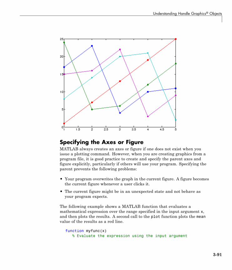
Understanding Handle Graphics® Objects
Specifying the Axes or FigureMATLAB always creates an axes or figure if one does not exist when youissue a plotting command. However, when you are creating graphics from aprogram file, it is good practice to create and specify the parent axes andfigure explicitly, particularly if others will use your program. Specifying theparent prevents the following problems:
• Your program overwrites the graph in the current figure. A figure becomesthe current figure whenever a user clicks it.
• The current figure might be in an unexpected state and not behave asyour program expects.
The following example shows a MATLAB function that evaluates amathematical expression over the range specified in the input argument x,and then plots the results. A second call to the plot function plots the meanvalue of the results as a red line.
function myfunc(x)% Evaluate the expression using the input argument
3-91
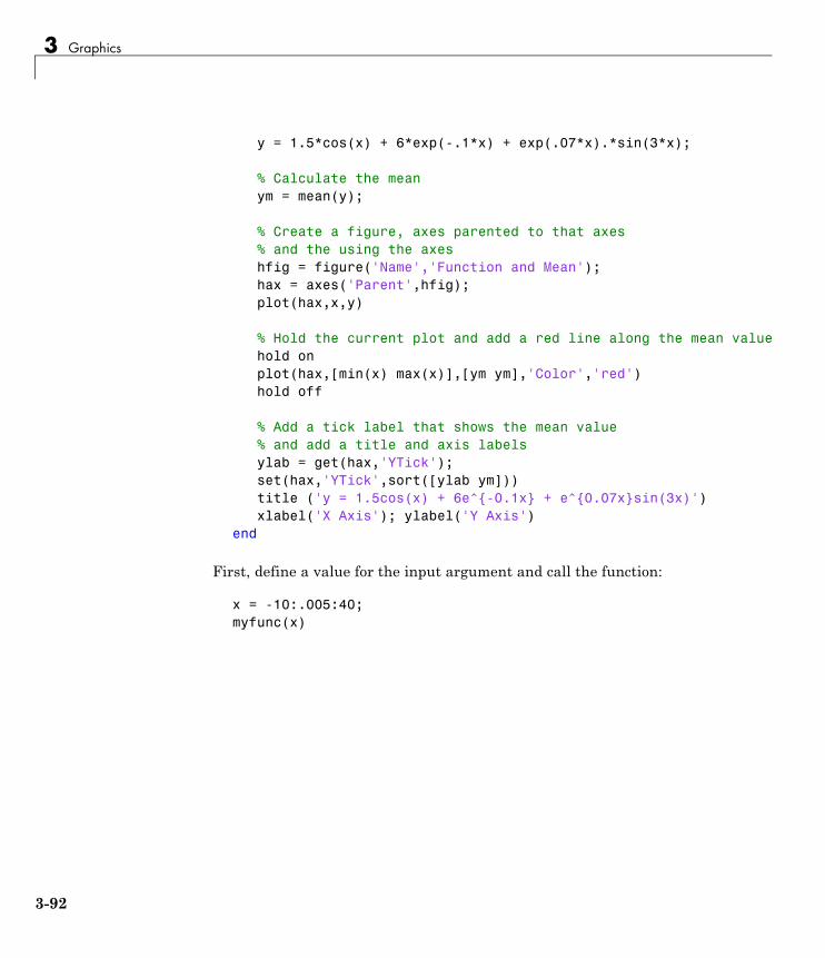
3 Graphics
y = 1.5*cos(x) + 6*exp(-.1*x) + exp(.07*x).*sin(3*x);
% Calculate the meanym = mean(y);
% Create a figure, axes parented to that axes% and the using the axeshfig = figure('Name','Function and Mean');hax = axes('Parent',hfig);plot(hax,x,y)
% Hold the current plot and add a red line along the mean valuehold onplot(hax,[min(x) max(x)],[ym ym],'Color','red')hold off
% Add a tick label that shows the mean value% and add a title and axis labelsylab = get(hax,'YTick');set(hax,'YTick',sort([ylab ym]))title ('y = 1.5cos(x) + 6e^{-0.1x} + e^{0.07x}sin(3x)')xlabel('X Axis'); ylabel('Y Axis')
end
First, define a value for the input argument and call the function:
x = -10:.005:40;myfunc(x)
3-92
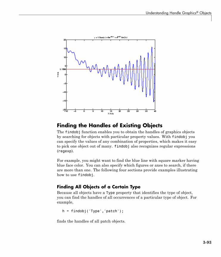
Understanding Handle Graphics® Objects
Finding the Handles of Existing ObjectsThe findobj function enables you to obtain the handles of graphics objectsby searching for objects with particular property values. With findobj youcan specify the values of any combination of properties, which makes it easyto pick one object out of many. findobj also recognizes regular expressions(regexp).
For example, you might want to find the blue line with square marker havingblue face color. You can also specify which figures or axes to search, if thereare more than one. The following four sections provide examples illustratinghow to use findobj.
Finding All Objects of a Certain TypeBecause all objects have a Type property that identifies the type of object,you can find the handles of all occurrences of a particular type of object. Forexample,
h = findobj('Type','patch');
finds the handles of all patch objects.
3-93
3 Graphics
Finding Objects with a Particular PropertyYou can specify multiple properties to narrow the search. For example,
h = findobj('Type','line','Color','r','LineStyle',':');
finds the handles of all red dotted lines.
Limiting the Scope of the SearchYou can specify the starting point in the object hierarchy by passing thehandle of the starting figure or axes as the first argument. For example,
h = findobj(gca,'Type','text','String','\pi/2');
finds the string π/2 only within the current axes.
Using findobj as an ArgumentBecause findobj returns the handles it finds, you can use it in place of thehandle argument. For example,
set(findobj('Type','line','Color','red'),'LineStyle',':')
finds all red lines and sets their line style to dotted.
3-94
4
Programming
If you have an active Internet Explorer® connection, you can watch the Writinga MATLAB Program video demo for an overview of the major functionality.
• “Flow Control” on page 4-2
• “Other Data Structures” on page 4-9
• “Scripts and Functions” on page 4-20
• “Object-Oriented Programming” on page 4-33
4 Programming
Flow Control
In this section...
“Conditional Control — if, else, switch” on page 4-2
“Loop Control — for, while, continue, break” on page 4-5
“Error Control — try, catch” on page 4-7
“Program Termination — return” on page 4-8
Conditional Control — if, else, switchConditional statements enable you to select at run time which block of code toexecute. The simplest conditional statement is an if statement. For example:
% Generate a random numbera = randi(100, 1);
% If it is even, divide by 2if rem(a, 2) == 0
disp('a is even')b = a/2;
end
if statements can include alternate choices, using the optional keywordselseif or else. For example:
a = randi(100, 1);
if a < 30disp('small')
elseif a < 80disp('medium')
elsedisp('large')
end
Alternatively, when you want to test for equality against a set of knownvalues, use a switch statement. For example:
4-2
Flow Control
[dayNum, dayString] = weekday(date, 'long', 'en_US');
switch dayStringcase 'Monday'
disp('Start of the work week')case 'Tuesday'
disp('Day 2')case 'Wednesday'
disp('Day 3')case 'Thursday'
disp('Day 4')case 'Friday'
disp('Last day of the work week')otherwise
disp('Weekend!')end
For both if and switch, MATLAB executes the code corresponding to thefirst true condition, and then exits the code block. Each conditional statementrequires the end keyword.
In general, when you have many possible discrete, known values, switchstatements are easier to read than if statements. However, you cannot testfor inequality between switch and case values. For example, you cannotimplement this type of condition with a switch:
yourNumber = input('Enter a number: ');
if yourNumber < 0disp('Negative')
elseif yourNumber > 0disp('Positive')
elsedisp('Zero')
end
Array Comparisons in Conditional StatementsIt is important to understand how relational operators and if statementswork with matrices. When you want to check for equality between twovariables, you might use
4-3
4 Programming
if A == B, ...
This is valid MATLAB code, and does what you expect when A and B arescalars. But when A and B are matrices, A == B does not test if they areequal, it tests where they are equal; the result is another matrix of 0’s and 1’sshowing element-by-element equality. (In fact, if A and B are not the samesize, then A == B is an error.)
A = magic(4); B = A; B(1,1) = 0;
A == Bans =
0 1 1 11 1 1 11 1 1 11 1 1 1
The proper way to check for equality between two variables is to use theisequal function:
if isequal(A, B), ...
isequal returns a scalar logical value of 1 (representing true) or 0 (false),instead of a matrix, as the expression to be evaluated by the if function.Using the A and B matrices from above, you get
isequal(A, B)ans =
0
Here is another example to emphasize this point. If A and B are scalars, thefollowing program will never reach the “unexpected situation”. But for mostpairs of matrices, including our magic squares with interchanged columns,none of the matrix conditions A > B, A < B, or A == B is true for all elementsand so the else clause is executed:
if A > B'greater'
elseif A < B'less'
elseif A == B'equal'
4-4
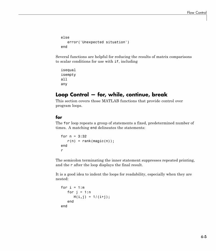
Flow Control
elseerror('Unexpected situation')
end
Several functions are helpful for reducing the results of matrix comparisonsto scalar conditions for use with if, including
isequalisemptyallany
Loop Control — for, while, continue, breakThis section covers those MATLAB functions that provide control overprogram loops.
forThe for loop repeats a group of statements a fixed, predetermined number oftimes. A matching end delineates the statements:
for n = 3:32r(n) = rank(magic(n));
endr
The semicolon terminating the inner statement suppresses repeated printing,and the r after the loop displays the final result.
It is a good idea to indent the loops for readability, especially when they arenested:
for i = 1:mfor j = 1:n
H(i,j) = 1/(i+j);end
end
4-5
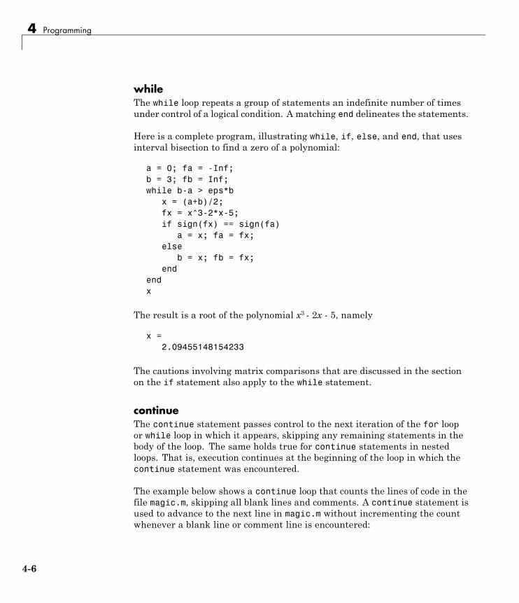
4 Programming
whileThe while loop repeats a group of statements an indefinite number of timesunder control of a logical condition. A matching end delineates the statements.
Here is a complete program, illustrating while, if, else, and end, that usesinterval bisection to find a zero of a polynomial:
a = 0; fa = -Inf;b = 3; fb = Inf;while b-a > eps*b
x = (a+b)/2;fx = x^3-2*x-5;if sign(fx) == sign(fa)
a = x; fa = fx;else
b = x; fb = fx;end
endx
The result is a root of the polynomial x3 - 2x - 5, namely
x =2.09455148154233
The cautions involving matrix comparisons that are discussed in the sectionon the if statement also apply to the while statement.
continueThe continue statement passes control to the next iteration of the for loopor while loop in which it appears, skipping any remaining statements in thebody of the loop. The same holds true for continue statements in nestedloops. That is, execution continues at the beginning of the loop in which thecontinue statement was encountered.
The example below shows a continue loop that counts the lines of code in thefile magic.m, skipping all blank lines and comments. A continue statement isused to advance to the next line in magic.m without incrementing the countwhenever a blank line or comment line is encountered:
4-6
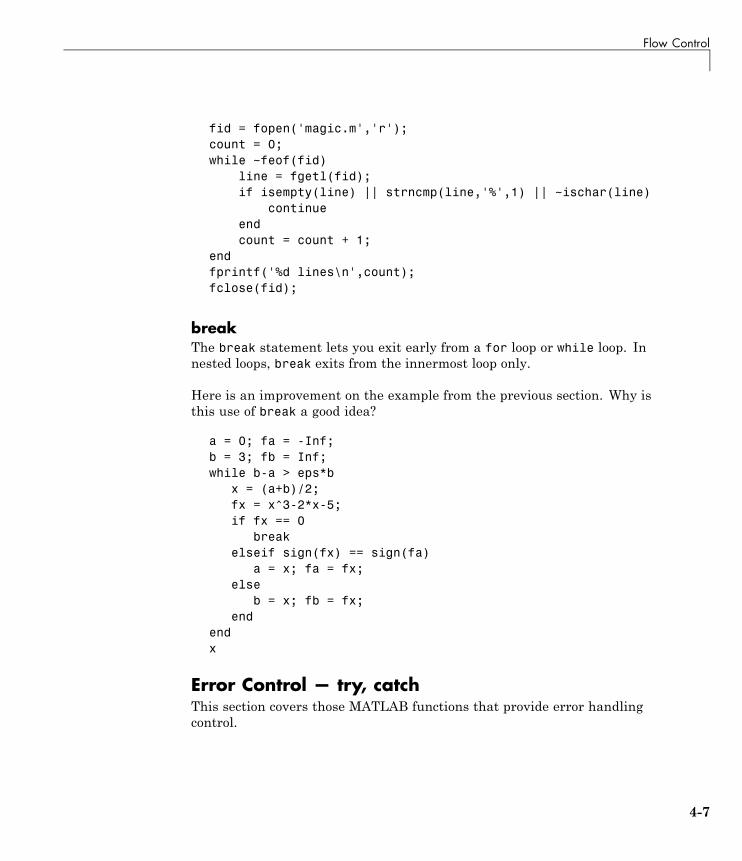
Flow Control
fid = fopen('magic.m','r');count = 0;while ~feof(fid)
line = fgetl(fid);if isempty(line) || strncmp(line,'%',1) || ~ischar(line)
continueendcount = count + 1;
endfprintf('%d lines\n',count);fclose(fid);
breakThe break statement lets you exit early from a for loop or while loop. Innested loops, break exits from the innermost loop only.
Here is an improvement on the example from the previous section. Why isthis use of break a good idea?
a = 0; fa = -Inf;b = 3; fb = Inf;while b-a > eps*b
x = (a+b)/2;fx = x^3-2*x-5;if fx == 0
breakelseif sign(fx) == sign(fa)
a = x; fa = fx;else
b = x; fb = fx;end
endx
Error Control — try, catchThis section covers those MATLAB functions that provide error handlingcontrol.
4-7
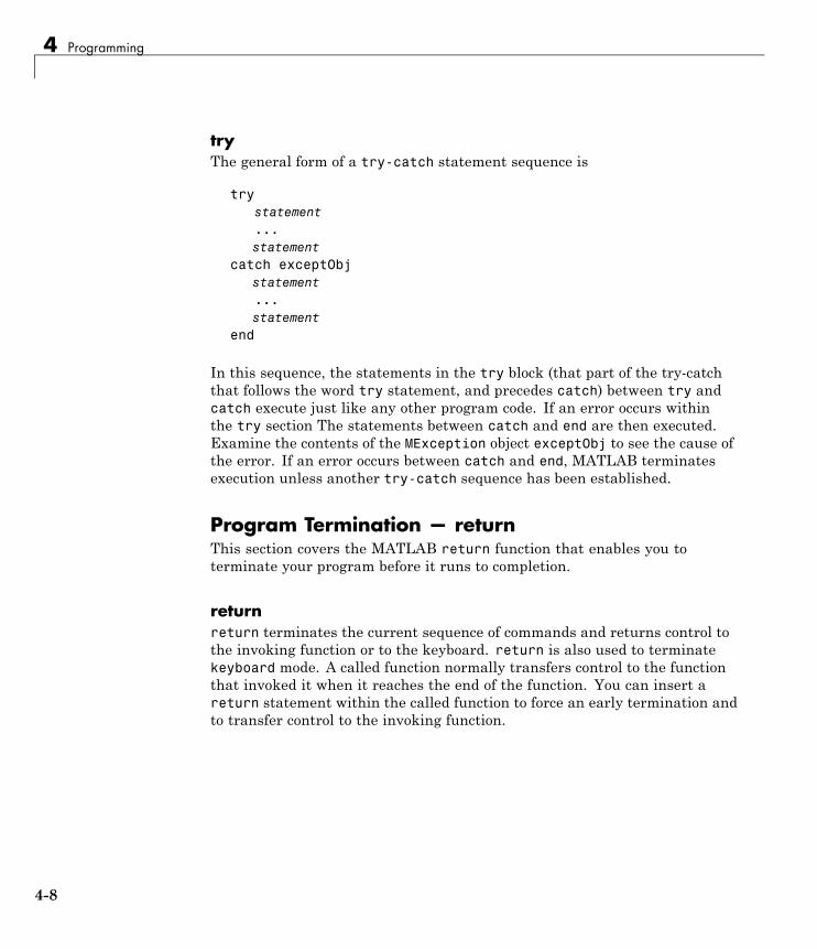
4 Programming
tryThe general form of a try-catch statement sequence is
trystatement...statement
catch exceptObjstatement...statement
end
In this sequence, the statements in the try block (that part of the try-catchthat follows the word try statement, and precedes catch) between try andcatch execute just like any other program code. If an error occurs withinthe try section The statements between catch and end are then executed.Examine the contents of the MException object exceptObj to see the cause ofthe error. If an error occurs between catch and end, MATLAB terminatesexecution unless another try-catch sequence has been established.
Program Termination — returnThis section covers the MATLAB return function that enables you toterminate your program before it runs to completion.
returnreturn terminates the current sequence of commands and returns control tothe invoking function or to the keyboard. return is also used to terminatekeyboard mode. A called function normally transfers control to the functionthat invoked it when it reaches the end of the function. You can insert areturn statement within the called function to force an early termination andto transfer control to the invoking function.
4-8
Other Data Structures
Other Data Structures
In this section...
“Multidimensional Arrays” on page 4-9
“Cell Arrays” on page 4-11
“Characters and Text” on page 4-13
“Structures” on page 4-16
Multidimensional ArraysMultidimensional arrays in the MATLAB environment are arrays with morethan two subscripts. One way of creating a multidimensional array is bycalling zeros, ones, rand, or randn with more than two arguments. Forexample,
R = randn(3,4,5);
creates a 3-by-4-by-5 array with a total of 3*4*5 = 60 normally distributedrandom elements.
A three-dimensional array might represent three-dimensional physical data,say the temperature in a room, sampled on a rectangular grid. Or it mightrepresent a sequence of matrices, A(k), or samples of a time-dependent matrix,A(t). In these latter cases, the (i, j)th element of the kth matrix, or the tkthmatrix, is denoted by A(i,j,k).
MATLAB and Dürer’s versions of the magic square of order 4 differ by aninterchange of two columns. Many different magic squares can be generatedby interchanging columns. The statement
p = perms(1:4);
generates the 4! = 24 permutations of 1:4. The kth permutation is the rowvector p(k,:). Then
A = magic(4);M = zeros(4,4,24);
4-9
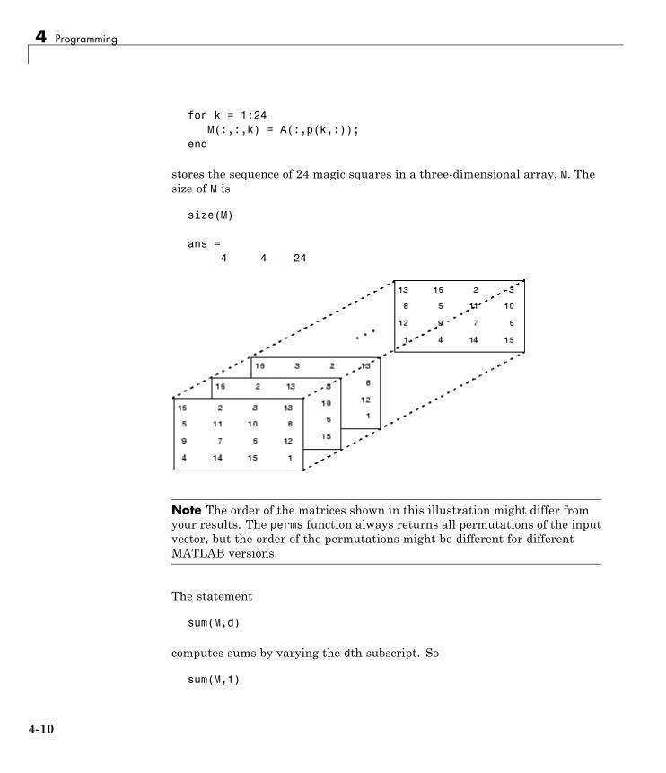
4 Programming
for k = 1:24M(:,:,k) = A(:,p(k,:));
end
stores the sequence of 24 magic squares in a three-dimensional array, M. Thesize of M is
size(M)
ans =4 4 24
Note The order of the matrices shown in this illustration might differ fromyour results. The perms function always returns all permutations of the inputvector, but the order of the permutations might be different for differentMATLAB versions.
The statement
sum(M,d)
computes sums by varying the dth subscript. So
sum(M,1)
4-10
Other Data Structures
is a 1-by-4-by-24 array containing 24 copies of the row vector
34 34 34 34
and
sum(M,2)
is a 4-by-1-by-24 array containing 24 copies of the column vector
34343434
Finally,
S = sum(M,3)
adds the 24 matrices in the sequence. The result has size 4-by-4-by-1, soit looks like a 4-by-4 array:
S =204 204 204 204204 204 204 204204 204 204 204204 204 204 204
Cell ArraysCell arrays in MATLAB are multidimensional arrays whose elements arecopies of other arrays. A cell array of empty matrices can be created withthe cell function. But, more often, cell arrays are created by enclosing amiscellaneous collection of things in curly braces, {}. The curly braces arealso used with subscripts to access the contents of various cells. For example,
C = {A sum(A) prod(prod(A))}
produces a 1-by-3 cell array. The three cells contain the magic square, therow vector of column sums, and the product of all its elements. When Cis displayed, you see
C =
4-11
4 Programming
[4x4 double] [1x4 double] [20922789888000]
This is because the first two cells are too large to print in this limited space,but the third cell contains only a single number, 16!, so there is room toprint it.
Here are two important points to remember. First, to retrieve the contents ofone of the cells, use subscripts in curly braces. For example, C{1} retrievesthe magic square and C{3} is 16!. Second, cell arrays contain copies of otherarrays, not pointers to those arrays. If you subsequently change A, nothinghappens to C.
You can use three-dimensional arrays to store a sequence of matrices of thesame size. Cell arrays can be used to store a sequence of matrices of differentsizes. For example,
M = cell(8,1);for n = 1:8
M{n} = magic(n);endM
produces a sequence of magic squares of different order:
M =[ 1][ 2x2 double][ 3x3 double][ 4x4 double][ 5x5 double][ 6x6 double][ 7x7 double][ 8x8 double]
4-12
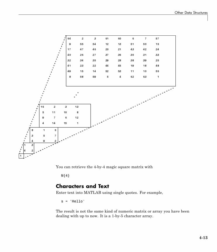
Other Data Structures
You can retrieve the 4-by-4 magic square matrix with
M{4}
Characters and TextEnter text into MATLAB using single quotes. For example,
s = 'Hello'
The result is not the same kind of numeric matrix or array you have beendealing with up to now. It is a 1-by-5 character array.
4-13
4 Programming
Internally, the characters are stored as numbers, but not in floating-pointformat. The statement
a = double(s)
converts the character array to a numeric matrix containing floating-pointrepresentations of the ASCII codes for each character. The result is
a =72 101 108 108 111
The statement
s = char(a)
reverses the conversion.
Converting numbers to characters makes it possible to investigate the variousfonts available on your computer. The printable characters in the basic ASCIIcharacter set are represented by the integers 32:127. (The integers less than32 represent nonprintable control characters.) These integers are arranged inan appropriate 6-by-16 array with
F = reshape(32:127,16,6)';
The printable characters in the extended ASCII character set are representedby F+128. When these integers are interpreted as characters, the resultdepends on the font currently being used. Type the statements
char(F)char(F+128)
and then vary the font being used for the Command Window. SelectPreferences from the File menu and then click Fonts to change the font. Ifyou include tabs in lines of code, use a fixed-width font, such as Monospaced,to align the tab positions on different lines.
Concatenation with square brackets joins text variables together into largerstrings. The statement
h = [s, ' world']
4-14
Other Data Structures
joins the strings horizontally and produces
h =Hello world
The statement
v = [s; 'world']
joins the strings vertically and produces
v =Helloworld
Note that a blank has to be inserted before the 'w' in h and that both wordsin v have to have the same length. The resulting arrays are both characterarrays; h is 1-by-11 and v is 2-by-5.
To manipulate a body of text containing lines of different lengths, you havetwo choices—a padded character array or a cell array of strings. Whencreating a character array, you must make each row of the array the samelength. (Pad the ends of the shorter rows with spaces.) The char function doesthis padding for you. For example,
S = char('A','rolling','stone','gathers','momentum.')
produces a 5-by-9 character array:
S =Arollingstonegathersmomentum.
Alternatively, you can store the text in a cell array. For example,
C = {'A';'rolling';'stone';'gathers';'momentum.'}
creates a 5-by-1 cell array that requires no padding because each row of thearray can have a different length:
4-15

4 Programming
C ='A''rolling''stone''gathers''momentum.'
You can convert a padded character array to a cell array of strings with
C = cellstr(S)
and reverse the process with
S = char(C)
StructuresStructures are multidimensional MATLAB arrays with elements accessed bytextual field designators. For example,
S.name = 'Ed Plum';S.score = 83;S.grade = 'B+'
creates a scalar structure with three fields:
S =name: 'Ed Plum'
score: 83grade: 'B+'
Like everything else in the MATLAB environment, structures are arrays, soyou can insert additional elements. In this case, each element of the array is astructure with several fields. The fields can be added one at a time,
S(2).name = 'Toni Miller';S(2).score = 91;S(2).grade = 'A-';
or an entire element can be added with a single statement:
S(3) = struct('name','Jerry Garcia',...'score',70,'grade','C')
4-16
Other Data Structures
Now the structure is large enough that only a summary is printed:
S =1x3 struct array with fields:
namescoregrade
There are several ways to reassemble the various fields into other MATLABarrays. They are mostly based on the notation of a comma-separated list. Ifyou type
S.score
it is the same as typing
S(1).score, S(2).score, S(3).score
which is a comma-separated list.
If you enclose the expression that generates such a list within squarebrackets, MATLAB stores each item from the list in an array. In this example,MATLAB creates a numeric row vector containing the score field of eachelement of structure array S:
scores = [S.score]scores =
83 91 70
avg_score = sum(scores)/length(scores)avg_score =
81.3333
To create a character array from one of the text fields (name, for example), callthe char function on the comma-separated list produced by S.name:
names = char(S.name)names =
Ed PlumToni MillerJerry Garcia
4-17
4 Programming
Similarly, you can create a cell array from the name fields by enclosing thelist-generating expression within curly braces:
names = {S.name}names =
'Ed Plum' 'Toni Miller' 'Jerry Garcia'
To assign the fields of each element of a structure array to separate variablesoutside of the structure, specify each output to the left of the equals sign,enclosing them all within square brackets:
[N1 N2 N3] = S.nameN1 =
Ed PlumN2 =
Toni MillerN3 =
Jerry Garcia
Dynamic Field NamesThe most common way to access the data in a structure is by specifying thename of the field that you want to reference. Another means of accessingstructure data is to use dynamic field names. These names express thefield as a variable expression that MATLAB evaluates at run-time. Thedot-parentheses syntax shown here makes expression a dynamic field name:
structName.(expression)
Index into this field using the standard MATLAB indexing syntax. Forexample, to evaluate expression into a field name and obtain the values ofthat field at columns 1 through 25 of row 7, use
structName.(expression)(7,1:25)
Dynamic Field Names Example. The avgscore function shown belowcomputes an average test score, retrieving information from the testscoresstructure using dynamic field names:
function avg = avgscore(testscores, student, first, last)for k = first:last
scores(k) = testscores.(student).week(k);
4-18
Other Data Structures
endavg = sum(scores)/(last - first + 1);
You can run this function using different values for the dynamic field student.First, initialize the structure that contains scores for a 25-week period:
testscores.Ann_Lane.week(1:25) = ...[95 89 76 82 79 92 94 92 89 81 75 93 ...85 84 83 86 85 90 82 82 84 79 96 88 98];
testscores.William_King.week(1:25) = ...[87 80 91 84 99 87 93 87 97 87 82 89 ...86 82 90 98 75 79 92 84 90 93 84 78 81];
Now run avgscore, supplying the students name fields for the testscoresstructure at runtime using dynamic field names:
avgscore(testscores, 'Ann_Lane', 7, 22)ans =
85.2500
avgscore(testscores, 'William_King', 7, 22)ans =
87.7500
4-19

4 Programming
Scripts and Functions
In this section...
“Overview” on page 4-20
“Scripts” on page 4-21
“Functions” on page 4-22
“Types of Functions” on page 4-24
“Global Variables” on page 4-26
“Passing String Arguments to Functions” on page 4-27
“The eval Function” on page 4-28
“Function Handles” on page 4-28
“Function Functions” on page 4-29
“Vectorization” on page 4-31
“Preallocation” on page 4-32
OverviewThe MATLAB product provides a powerful programming language, as well asan interactive computational environment. You can enter commands fromthe language one at a time at the MATLAB command line, or you can write aseries of commands to a file that you then execute as you would any MATLABfunction. Use the MATLAB Editor or any other text editor to create yourown function files. Call these functions as you would any other MATLABfunction or command.
There are two kinds of program files:
• Scripts, which do not accept input arguments or return output arguments.They operate on data in the workspace.
• Functions, which can accept input arguments and return outputarguments. Internal variables are local to the function.
If you are a new MATLAB programmer, just create the program files that youwant to try out in the current folder. As you develop more of your own files,
4-20
Scripts and Functions
you will want to organize them into other folders and personal toolboxes thatyou can add to your MATLAB search path.
If you duplicate function names, MATLAB executes the one that occurs firstin the search path.
To view the contents of a program file, for example, myfunction.m, use
type myfunction
For more detailed information, see “Functions and Scripts” in the MATLABProgramming Fundamentals documentation.
ScriptsWhen you invoke a script, MATLAB simply executes the commands found inthe file. Scripts can operate on existing data in the workspace, or they cancreate new data on which to operate. Although scripts do not return outputarguments, any variables that they create remain in the workspace, to beused in subsequent computations. In addition, scripts can produce graphicaloutput using functions like plot.
For example, create a file called magicrank.m that contains these MATLABcommands:
% Investigate the rank of magic squaresr = zeros(1,32);for n = 3:32
r(n) = rank(magic(n));endrbar(r)
Typing the statement
magicrank
causes MATLAB to execute the commands, compute the rank of the first 30magic squares, and plot a bar graph of the result. After execution of the file iscomplete, the variables n and r remain in the workspace.
4-21
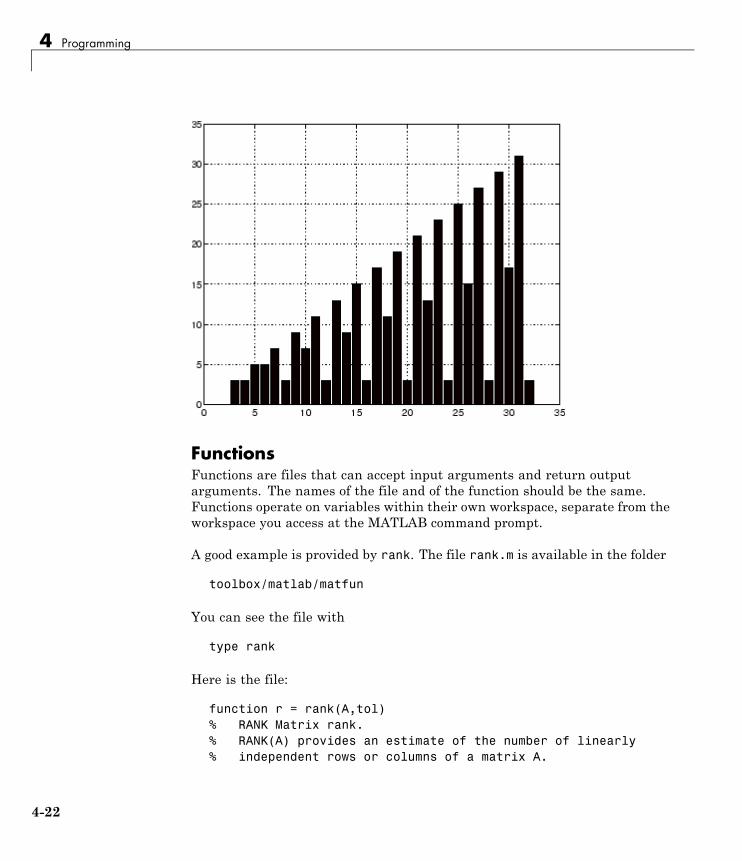
4 Programming
FunctionsFunctions are files that can accept input arguments and return outputarguments. The names of the file and of the function should be the same.Functions operate on variables within their own workspace, separate from theworkspace you access at the MATLAB command prompt.
A good example is provided by rank. The file rank.m is available in the folder
toolbox/matlab/matfun
You can see the file with
type rank
Here is the file:
function r = rank(A,tol)% RANK Matrix rank.% RANK(A) provides an estimate of the number of linearly% independent rows or columns of a matrix A.
4-22
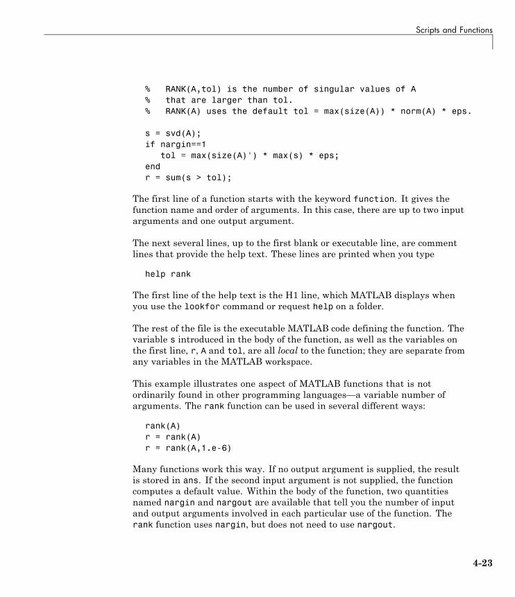
Scripts and Functions
% RANK(A,tol) is the number of singular values of A% that are larger than tol.% RANK(A) uses the default tol = max(size(A)) * norm(A) * eps.
s = svd(A);if nargin==1
tol = max(size(A)') * max(s) * eps;endr = sum(s > tol);
The first line of a function starts with the keyword function. It gives thefunction name and order of arguments. In this case, there are up to two inputarguments and one output argument.
The next several lines, up to the first blank or executable line, are commentlines that provide the help text. These lines are printed when you type
help rank
The first line of the help text is the H1 line, which MATLAB displays whenyou use the lookfor command or request help on a folder.
The rest of the file is the executable MATLAB code defining the function. Thevariable s introduced in the body of the function, as well as the variables onthe first line, r, A and tol, are all local to the function; they are separate fromany variables in the MATLAB workspace.
This example illustrates one aspect of MATLAB functions that is notordinarily found in other programming languages—a variable number ofarguments. The rank function can be used in several different ways:
rank(A)r = rank(A)r = rank(A,1.e-6)
Many functions work this way. If no output argument is supplied, the resultis stored in ans. If the second input argument is not supplied, the functioncomputes a default value. Within the body of the function, two quantitiesnamed nargin and nargout are available that tell you the number of inputand output arguments involved in each particular use of the function. Therank function uses nargin, but does not need to use nargout.
4-23
4 Programming
Types of FunctionsMATLAB offers several different types of functions to use in yourprogramming.
Anonymous FunctionsAn anonymous function is a simple form of the MATLAB function that isdefined within a single MATLAB statement. It consists of a single MATLABexpression and any number of input and output arguments. You can definean anonymous function right at the MATLAB command line, or within afunction or script. This gives you a quick means of creating simple functionswithout having to create a file for them each time.
The syntax for creating an anonymous function from an expression is
f = @(arglist)expression
The statement below creates an anonymous function that finds the square ofa number. When you call this function, MATLAB assigns the value you passin to variable x, and then uses x in the equation x.^2:
sqr = @(x) x.^2;
To execute the sqr function defined above, type
a = sqr(5)a =
25
Primary and SubfunctionsAny function that is not anonymous must be defined within a file. Each suchfunction file contains a required primary function that appears first, and anynumber of subfunctions that may follow the primary. Primary functions havea wider scope than subfunctions. That is, primary functions can be calledfrom outside of the file that defines them (e.g., from the MATLAB commandline or from functions in other files) while subfunctions cannot. Subfunctionsare visible only to the primary function and other subfunctions within theirown file.
4-24
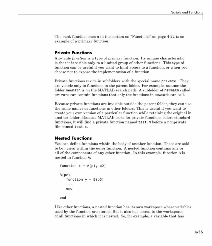
Scripts and Functions
The rank function shown in the section on “Functions” on page 4-22 is anexample of a primary function.
Private FunctionsA private function is a type of primary function. Its unique characteristicis that it is visible only to a limited group of other functions. This type offunction can be useful if you want to limit access to a function, or when youchoose not to expose the implementation of a function.
Private functions reside in subfolders with the special name private. Theyare visible only to functions in the parent folder. For example, assume thefolder newmath is on the MATLAB search path. A subfolder of newmath calledprivate can contain functions that only the functions in newmath can call.
Because private functions are invisible outside the parent folder, they can usethe same names as functions in other folders. This is useful if you want tocreate your own version of a particular function while retaining the original inanother folder. Because MATLAB looks for private functions before standardfunctions, it will find a private function named test.m before a nonprivatefile named test.m.
Nested FunctionsYou can define functions within the body of another function. These are saidto be nested within the outer function. A nested function contains any orall of the components of any other function. In this example, function B isnested in function A:
function x = A(p1, p2)...B(p2)
function y = B(p3)...end
...end
Like other functions, a nested function has its own workspace where variablesused by the function are stored. But it also has access to the workspacesof all functions in which it is nested. So, for example, a variable that has
4-25
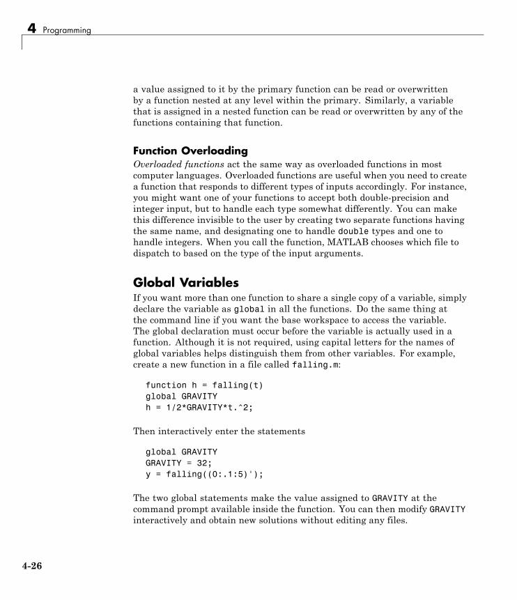
4 Programming
a value assigned to it by the primary function can be read or overwrittenby a function nested at any level within the primary. Similarly, a variablethat is assigned in a nested function can be read or overwritten by any of thefunctions containing that function.
Function OverloadingOverloaded functions act the same way as overloaded functions in mostcomputer languages. Overloaded functions are useful when you need to createa function that responds to different types of inputs accordingly. For instance,you might want one of your functions to accept both double-precision andinteger input, but to handle each type somewhat differently. You can makethis difference invisible to the user by creating two separate functions havingthe same name, and designating one to handle double types and one tohandle integers. When you call the function, MATLAB chooses which file todispatch to based on the type of the input arguments.
Global VariablesIf you want more than one function to share a single copy of a variable, simplydeclare the variable as global in all the functions. Do the same thing atthe command line if you want the base workspace to access the variable.The global declaration must occur before the variable is actually used in afunction. Although it is not required, using capital letters for the names ofglobal variables helps distinguish them from other variables. For example,create a new function in a file called falling.m:
function h = falling(t)global GRAVITYh = 1/2*GRAVITY*t.^2;
Then interactively enter the statements
global GRAVITYGRAVITY = 32;y = falling((0:.1:5)');
The two global statements make the value assigned to GRAVITY at thecommand prompt available inside the function. You can then modify GRAVITYinteractively and obtain new solutions without editing any files.
4-26
Scripts and Functions
Passing String Arguments to FunctionsYou can write MATLAB functions that accept string arguments without theparentheses and quotes. That is, MATLAB interprets
foo a b c
as
foo('a','b','c')
However, when you use the unquoted form, MATLAB cannot return outputarguments. For example,
legend apples oranges
creates a legend on a plot using the strings apples and oranges as labels.If you want the legend command to return its output arguments, then youmust use the quoted form:
[legh,objh] = legend('apples','oranges');
In addition, you must use the quoted form if any of the arguments is nota string.
Caution While the unquoted syntax is convenient, in some cases it can beused incorrectly without causing MATLAB to generate an error.
Constructing String Arguments in CodeThe quoted form enables you to construct string arguments within thecode. The following example processes multiple data files, August1.dat,August2.dat, and so on. It uses the function int2str, which converts aninteger to a character, to build the filename:
for d = 1:31s = ['August' int2str(d) '.dat'];load(s)% Code to process the contents of the d-th file
end
4-27
4 Programming
The eval FunctionThe eval function works with text variables to implement a powerful textmacro facility. The expression or statement
eval(s)
uses the MATLAB interpreter to evaluate the expression or execute thestatement contained in the text string s.
The example of the previous section could also be done with the followingcode, although this would be somewhat less efficient because it involves thefull interpreter, not just a function call:
for d = 1:31s = ['load August' int2str(d) '.dat'];eval(s)% Process the contents of the d-th file
end
Function HandlesYou can create a handle to any MATLAB function and then use that handleas a means of referencing the function. A function handle is typically passedin an argument list to other functions, which can then execute, or evaluate,the function using the handle.
Construct a function handle in MATLAB using the at sign, @, before thefunction name. The following example creates a function handle for the sinfunction and assigns it to the variable fhandle:
fhandle = @sin;
You can call a function by means of its handle in the same way that you wouldcall the function using its name. The syntax is
fhandle(arg1, arg2, ...);
The function plot_fhandle, shown below, receives a function handle anddata, generates y-axis data using the function handle, and plots it:
function plot_fhandle(fhandle, data)plot(data, fhandle(data))
4-28
Scripts and Functions
When you call plot_fhandle with a handle to the sin function and theargument shown below, the resulting evaluation produces a sine wave plot:
plot_fhandle(@sin, -pi:0.01:pi)
Function FunctionsA class of functions called “function functions” works with nonlinear functionsof a scalar variable. That is, one function works on another function. Thefunction functions include
• Zero finding
• Optimization
• Quadrature
• Ordinary differential equations
MATLAB represents the nonlinear function by the file that defines it.For example, here is a simplified version of the function humps from thematlab/demos folder:
function y = humps(x)y = 1./((x-.3).^2 + .01) + 1./((x-.9).^2 + .04) - 6;
Evaluate this function at a set of points in the interval 0 ≤ x ≤ 1 with
x = 0:.002:1;y = humps(x);
Then plot the function with
plot(x,y)
4-29
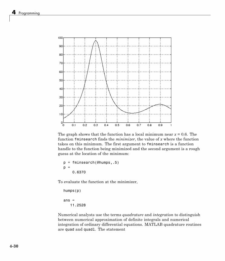
4 Programming
The graph shows that the function has a local minimum near x = 0.6. Thefunction fminsearch finds the minimizer, the value of x where the functiontakes on this minimum. The first argument to fminsearch is a functionhandle to the function being minimized and the second argument is a roughguess at the location of the minimum:
p = fminsearch(@humps,.5)p =
0.6370
To evaluate the function at the minimizer,
humps(p)
ans =11.2528
Numerical analysts use the terms quadrature and integration to distinguishbetween numerical approximation of definite integrals and numericalintegration of ordinary differential equations. MATLAB quadrature routinesare quad and quadl. The statement
4-30
Scripts and Functions
Q = quadl(@humps,0,1)
computes the area under the curve in the graph and produces
Q =29.8583
Finally, the graph shows that the function is never zero on this interval. So,if you search for a zero with
z = fzero(@humps,.5)
you will find one outside the interval
z =-0.1316
VectorizationOne way to make your MATLAB programs run faster is to vectorize thealgorithms you use in constructing the programs. Where other programminglanguages might use for loops or DO loops, MATLAB can use vector or matrixoperations. A simple example involves creating a table of logarithms:
x = .01;for k = 1:1001
y(k) = log10(x);x = x + .01;
end
A vectorized version of the same code is
x = .01:.01:10;y = log10(x);
For more complicated code, vectorization options are not always so obvious.
For More Information See “Performance” in the MATLAB ProgrammingFundamentals documentation for other techniques that you can use.
4-31
4 Programming
PreallocationIf you cannot vectorize a piece of code, you can make your for loops go fasterby preallocating any vectors or arrays in which output results are stored. Forexample, this code uses the function zeros to preallocate the vector created inthe for loop. This makes the for loop execute significantly faster:
r = zeros(32,1);for n = 1:32
r(n) = rank(magic(n));end
Without the preallocation in the previous example, the MATLAB interpreterenlarges the r vector by one element each time through the loop. Vectorpreallocation eliminates this step and results in faster execution.
4-32
Object-Oriented Programming
Object-Oriented Programming
In this section...
“MATLAB Classes and Objects” on page 4-33
“Learn About Defining MATLAB Classes” on page 4-33
MATLAB Classes and ObjectsMATLAB object-oriented programming capabilities enable you to develop andmaintain large application and define complex data structures that integrateseamlessly into the MATLAB environment. Some of the features include:
• Support for value and handle (reference) classes
• Definition of events and listeners
• Class introspection
• JIT/Accelerator support for classes to improve performance
Learn About Defining MATLAB ClassesFor complete information on using and creating MATLAB classes, seeObject-Oriented Programming in the user-guide documentation.
4-33

4 Programming
4-34
5
Data Analysis
• “Introduction” on page 5-2
• “Preprocessing Data” on page 5-3
• “Summarizing Data” on page 5-10
• “Visualizing Data” on page 5-14
• “Modeling Data” on page 5-27
5 Data Analysis
IntroductionEvery data analysis has some standard components:
• Preprocessing — Consider outliers and missing values, and smooth datato identify possible models.
• Summarizing — Compute basic statistics to describe the overall location,scale, and shape of the data.
• Visualizing — Plot data to identify patterns and trends.
• Modeling — Give data trends fuller descriptions, suitable for predictingnew values.
Data analysis moves among these components with two basic goals in mind:
1 Describe the patterns in the data with simple models that lead to accuratepredictions.
2 Understand the relationships among variables that lead to the model.
This section of the Getting Started guide explains how to carry out a basicdata analysis in the MATLAB environment.
5-2
Preprocessing Data
Preprocessing Data
In this section...
“Overview” on page 5-3
“Loading the Data” on page 5-3
“Missing Data” on page 5-3
“Outliers” on page 5-4
“Smoothing and Filtering” on page 5-6
OverviewBegin a data analysis by loading data into suitable MATLAB containervariables and sorting out the “good” data from the “bad.” This is a preliminarystep that assures meaningful conclusions in subsequent parts of the analysis.
Note This section begins a data analysis that is continued in “SummarizingData” on page 5-10, “Visualizing Data” on page 5-14, and “Modeling Data”on page 5-27.
Loading the DataBegin by loading the data in count.dat:
load count.dat
The 24-by-3 array count contains hourly traffic counts (the rows) at threeintersections (the columns) for a single day.
See “Importing and Exporting Data” in the MATLAB Data Analysisdocumentation for more information on storing data in MATLAB variablesfor analysis.
Missing DataThe MATLAB NaN (Not a Number) value is normally used to representmissing data. NaN values allow variables with missing data to maintain their
5-3

5 Data Analysis
structure—in this case, 24-by-1 vectors with consistent indexing across allthree intersections.
Check the data at the third intersection for NaN values using the isnanfunction:
c3 = count(:,3); % Data at intersection 3c3NaNCount = sum(isnan(c3))c3NaNCount =
0
isnan returns a logical vector the same size as c3, with entries indicating thepresence (1) or absence (0) of NaN values for each of the 24 elements in thedata. In this case, the logical values sum to 0, so there are no NaN valuesin the data.
NaN values are introduced into the data in the section on “Outliers” on page5-4.
See “Missing Data” in the MATLAB Data Analysis documentation for moreinformation on handling missing data.
OutliersOutliers are data values that are dramatically different from patterns inthe rest of the data. They may be due to measurement error, or they mayrepresent significant features in the data. Identifying outliers, and decidingwhat to do with them, depends on an understanding of the data and its source.
One common method for identifying outliers is to look for values more thana certain number of standard deviations σ from the mean μ. The followingcode plots a histogram of the data at the third intersection together with linesat μ and μ + nσ, for n = 1, 2:
bin_counts = hist(c3); % Histogram bin countsN = max(bin_counts); % Maximum bin countmu3 = mean(c3); % Data meansigma3 = std(c3); % Data standard deviation
hist(c3) % Plot histogramhold on
5-4
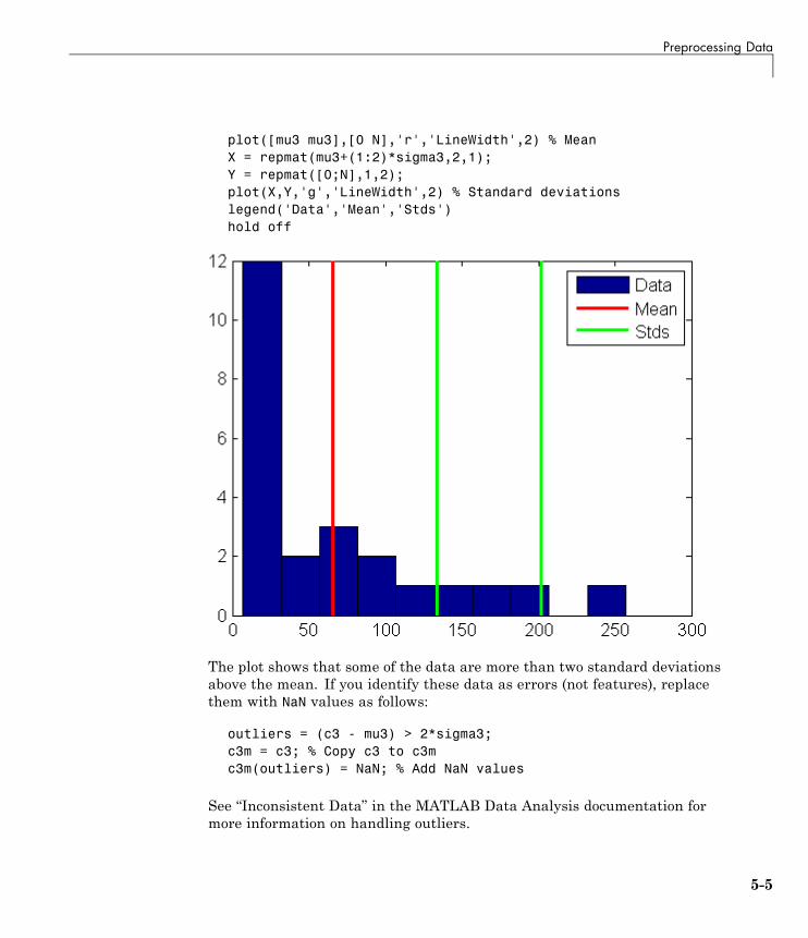
Preprocessing Data
plot([mu3 mu3],[0 N],'r','LineWidth',2) % MeanX = repmat(mu3+(1:2)*sigma3,2,1);Y = repmat([0;N],1,2);plot(X,Y,'g','LineWidth',2) % Standard deviationslegend('Data','Mean','Stds')hold off
The plot shows that some of the data are more than two standard deviationsabove the mean. If you identify these data as errors (not features), replacethem with NaN values as follows:
outliers = (c3 - mu3) > 2*sigma3;c3m = c3; % Copy c3 to c3mc3m(outliers) = NaN; % Add NaN values
See “Inconsistent Data” in the MATLAB Data Analysis documentation formore information on handling outliers.
5-5
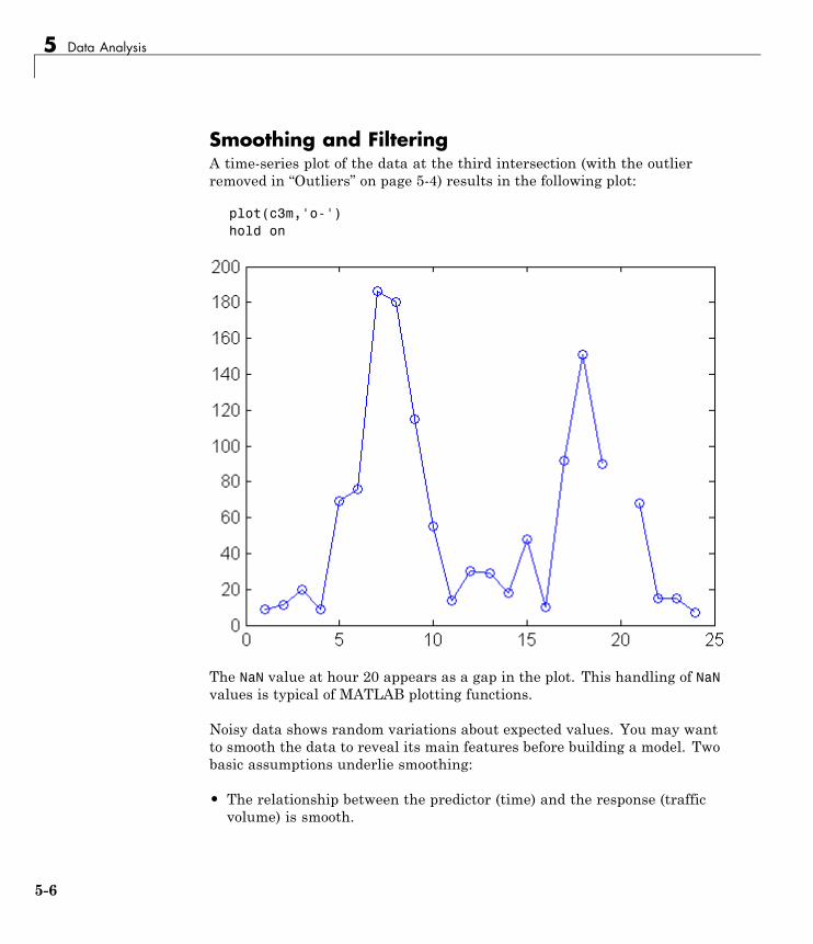
5 Data Analysis
Smoothing and FilteringA time-series plot of the data at the third intersection (with the outlierremoved in “Outliers” on page 5-4) results in the following plot:
plot(c3m,'o-')hold on
The NaN value at hour 20 appears as a gap in the plot. This handling of NaNvalues is typical of MATLAB plotting functions.
Noisy data shows random variations about expected values. You may wantto smooth the data to reveal its main features before building a model. Twobasic assumptions underlie smoothing:
• The relationship between the predictor (time) and the response (trafficvolume) is smooth.
5-6
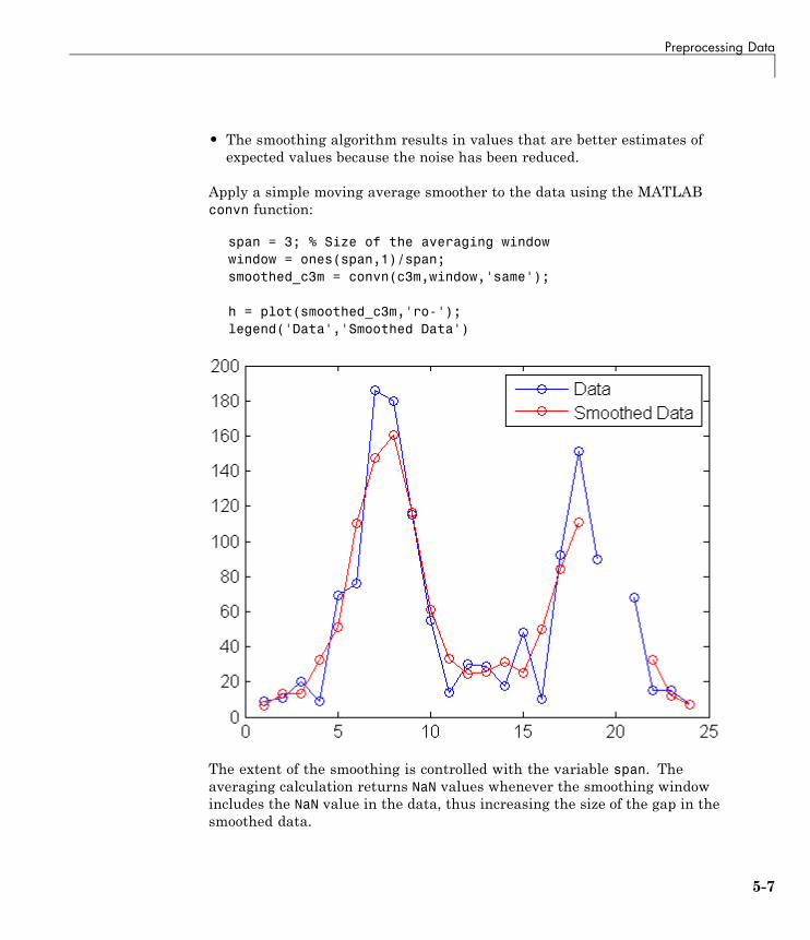
Preprocessing Data
• The smoothing algorithm results in values that are better estimates ofexpected values because the noise has been reduced.
Apply a simple moving average smoother to the data using the MATLABconvn function:
span = 3; % Size of the averaging windowwindow = ones(span,1)/span;smoothed_c3m = convn(c3m,window,'same');
h = plot(smoothed_c3m,'ro-');legend('Data','Smoothed Data')
The extent of the smoothing is controlled with the variable span. Theaveraging calculation returns NaN values whenever the smoothing windowincludes the NaN value in the data, thus increasing the size of the gap in thesmoothed data.
5-7
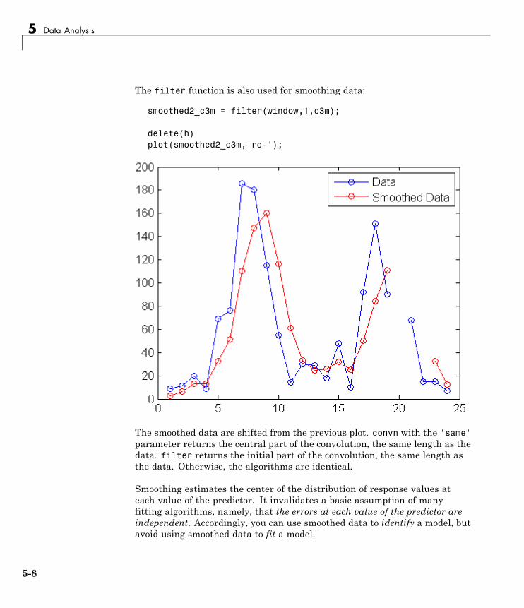
5 Data Analysis
The filter function is also used for smoothing data:
smoothed2_c3m = filter(window,1,c3m);
delete(h)plot(smoothed2_c3m,'ro-');
The smoothed data are shifted from the previous plot. convn with the 'same'parameter returns the central part of the convolution, the same length as thedata. filter returns the initial part of the convolution, the same length asthe data. Otherwise, the algorithms are identical.
Smoothing estimates the center of the distribution of response values ateach value of the predictor. It invalidates a basic assumption of manyfitting algorithms, namely, that the errors at each value of the predictor areindependent. Accordingly, you can use smoothed data to identify a model, butavoid using smoothed data to fit a model.
5-8
Preprocessing Data
See “Filtering Data” in the MATLAB Data Analysis documentation for moreinformation on smoothing and filtering.
5-9

5 Data Analysis
Summarizing Data
In this section...
“Overview” on page 5-10
“Measures of Location” on page 5-10
“Measures of Scale” on page 5-11
“Shape of a Distribution” on page 5-11
OverviewMany MATLAB functions enable you to summarize the overall location, scale,and shape of a data sample.
One of the advantages of working in MATLAB is that functions operate onentire arrays of data, not just on single scalar values. The functions are saidto be vectorized. Vectorization allows for both efficient problem formulation,using array-based data, and efficient computation, using vectorized statisticalfunctions.
Note This section continues the data analysis from “Preprocessing Data”on page 5-3.
Measures of LocationSummarize the location of a data sample by finding a “typical” value.Common measures of location or “central tendency” are computed by thefunctions mean, median, and mode:
load count.datx1 = mean(count)x1 =
32.0000 46.5417 65.5833
x2 = median(count)x2 =
23.5000 36.0000 39.0000
5-10
Summarizing Data
x3 = mode(count)x3 =
11 9 9
Like all of its statistical functions, the MATLAB functions above summarizedata across observations (rows) while preserving variables (columns). Thefunctions compute the location of the data at each of the three intersectionsin a single call.
Measures of ScaleThere are many ways to measure the scale or “dispersion” of a data sample.The MATLAB functions max, min, std, and var compute some commonmeasures:
dx1 = max(count)-min(count)dx1 =
107 136 250
dx2 = std(count)dx2 =
25.3703 41.4057 68.0281
dx3 = var(count)dx3 =
1.0e+003 *0.6437 1.7144 4.6278
Like all of its statistical functions, the MATLAB functions above summarizedata across observations (rows) while preserving variables (columns). Thefunctions compute the scale of the data at each of the three intersectionsin a single call.
Shape of a DistributionThe shape of a distribution is harder to summarize than its location orscale. The MATLAB hist function plots a histogram that provides a visualsummary:
figure
5-11

5 Data Analysis
hist(count)legend('Intersection 1',...
'Intersection 2',...'Intersection 3')
Parametric models give analytic summaries of distribution shapes.Exponential distributions, with parameter mu given by the data mean, are agood choice for the traffic data:
c1 = count(:,1); % Data at intersection 1[bin_counts,bin_locations] = hist(c1);bin_width = bin_locations(2) - bin_locations(1);hist_area = (bin_width)*(sum(bin_counts));
figurehist(c1)hold on
5-12
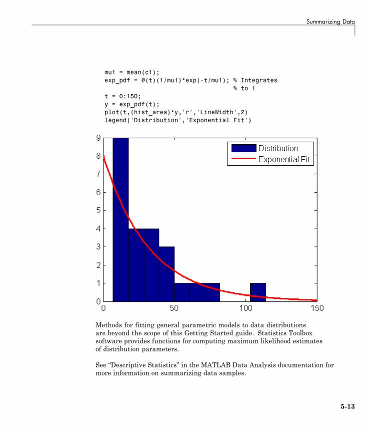
Summarizing Data
mu1 = mean(c1);exp_pdf = @(t)(1/mu1)*exp(-t/mu1); % Integrates
% to 1t = 0:150;y = exp_pdf(t);plot(t,(hist_area)*y,'r','LineWidth',2)legend('Distribution','Exponential Fit')
Methods for fitting general parametric models to data distributionsare beyond the scope of this Getting Started guide. Statistics Toolboxsoftware provides functions for computing maximum likelihood estimatesof distribution parameters.
See “Descriptive Statistics” in the MATLAB Data Analysis documentation formore information on summarizing data samples.
5-13
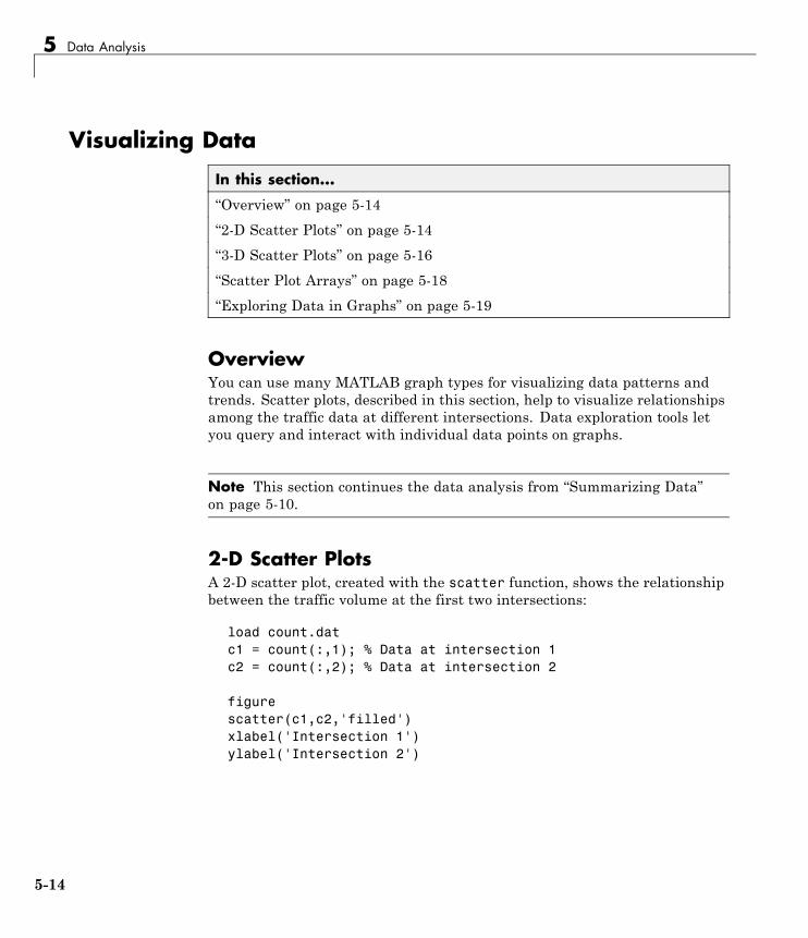
5 Data Analysis
Visualizing Data
In this section...
“Overview” on page 5-14
“2-D Scatter Plots” on page 5-14
“3-D Scatter Plots” on page 5-16
“Scatter Plot Arrays” on page 5-18
“Exploring Data in Graphs” on page 5-19
OverviewYou can use many MATLAB graph types for visualizing data patterns andtrends. Scatter plots, described in this section, help to visualize relationshipsamong the traffic data at different intersections. Data exploration tools letyou query and interact with individual data points on graphs.
Note This section continues the data analysis from “Summarizing Data”on page 5-10.
2-D Scatter PlotsA 2-D scatter plot, created with the scatter function, shows the relationshipbetween the traffic volume at the first two intersections:
load count.datc1 = count(:,1); % Data at intersection 1c2 = count(:,2); % Data at intersection 2
figurescatter(c1,c2,'filled')xlabel('Intersection 1')ylabel('Intersection 2')
5-14
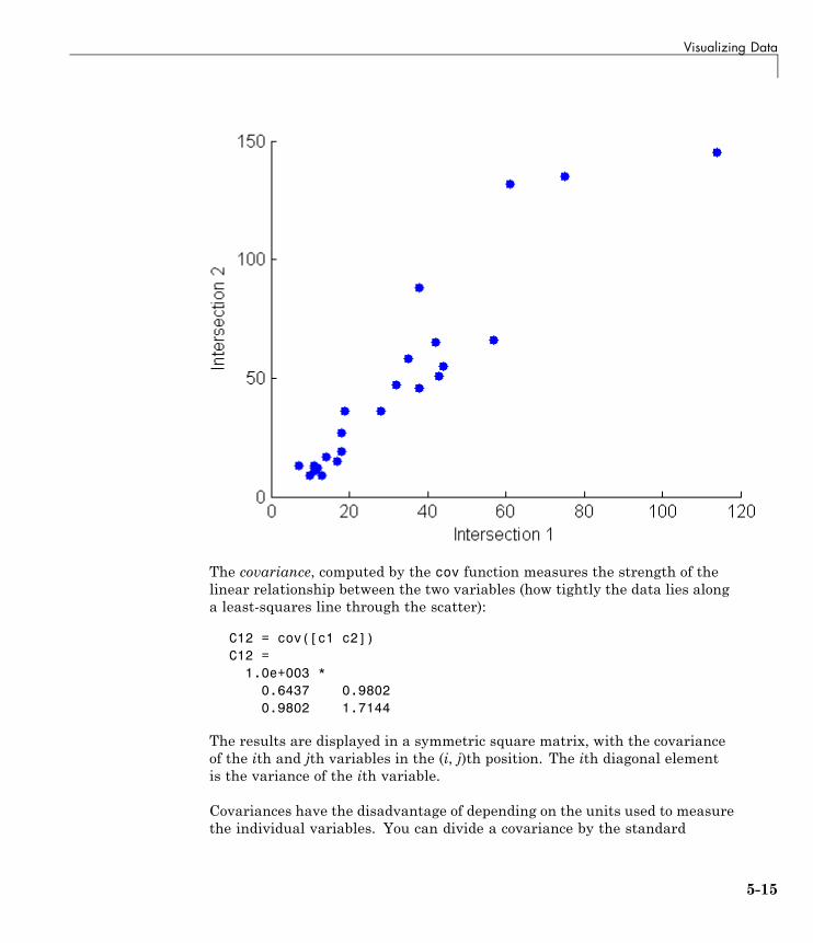
Visualizing Data
The covariance, computed by the cov function measures the strength of thelinear relationship between the two variables (how tightly the data lies alonga least-squares line through the scatter):
C12 = cov([c1 c2])C12 =
1.0e+003 *0.6437 0.98020.9802 1.7144
The results are displayed in a symmetric square matrix, with the covarianceof the ith and jth variables in the (i, j)th position. The ith diagonal elementis the variance of the ith variable.
Covariances have the disadvantage of depending on the units used to measurethe individual variables. You can divide a covariance by the standard
5-15
5 Data Analysis
deviations of the variables to normalize values between +1 and –1. Thecorrcoef function computes correlation coefficients:
R12 = corrcoef([c1 c2])R12 =
1.0000 0.93310.9331 1.0000
r12 = R12(1,2) % Correlation coefficientr12 =
0.9331
r12sq = r12^2 % Coefficient of determinationr12sq =
0.8707
Because it is normalized, the value of the correlation coefficient is readilycomparable to values for other pairs of intersections. Its square, the coefficientof determination, is the variance about the least-squares line divided bythe variance about the mean. Thus, it is the proportion of variation in theresponse (in this case, the traffic volume at intersection 2) that is eliminatedor statistically explained by a least-squares line through the scatter.
3-D Scatter PlotsA 3-D scatter plot, created with the scatter3 function, shows the relationshipbetween the traffic volume at all three intersections. Use the variables c1,c2, and c3 that you created in the previous step:
figurescatter3(c1,c2,c3,'filled')xlabel('Intersection 1')ylabel('Intersection 2')zlabel('Intersection 3')
5-16
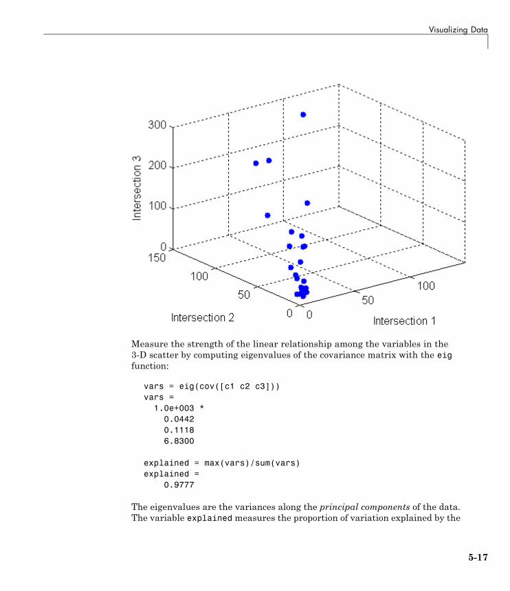
Visualizing Data
Measure the strength of the linear relationship among the variables in the3-D scatter by computing eigenvalues of the covariance matrix with the eigfunction:
vars = eig(cov([c1 c2 c3]))vars =
1.0e+003 *0.04420.11186.8300
explained = max(vars)/sum(vars)explained =
0.9777
The eigenvalues are the variances along the principal components of the data.The variable explainedmeasures the proportion of variation explained by the
5-17

5 Data Analysis
first principal component, along the axis of the data. Unlike the coefficientof determination for 2-D scatters, this measure distinguishes predictor andresponse variables.
Scatter Plot ArraysUse the plotmatrix function to make comparisons of the relationshipsbetween multiple pairs of intersections:
figureplotmatrix(count)
The plot in the (i, j)th position of the array is a scatter with the i th variableon the vertical axis and the jth variable on the horizontal axis. The plot in theith diagonal position is a histogram of the ith variable.
For more information on statistical visualization, see “Plotting Data” and“Interactive Data Exploration” in the MATLAB Data Analysis documentation.
5-18

Visualizing Data
Exploring Data in GraphsUsing your mouse, you can pick observations on almost any MATLAB graphwith two tools from the figure toolbar:
• Data Cursor
• Data Brushing
These tools each place you in exploratory modes in which you can select datapoints on graphs to identify their values and create workspace variables tocontain specific observations. When you use data brushing, you can also copy,remove or replace the selected observations.
For example, make a scatter plot of the first and third columns of count:
load count.datscatter(count(:,1),count(:,3))
Select the Data Cursor Tool and click the right-most data point. A datatipdisplaying the point’s x and y value is placed there.
5-19
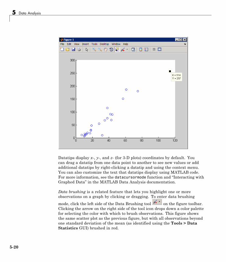
5 Data Analysis
Datatips display x-, y-, and z- (for 3-D plots) coordinates by default. Youcan drag a datatip from one data point to another to see new values or addadditional datatips by right-clicking a datatip and using the context menu.You can also customize the text that datatips display using MATLAB code.For more information, see the datacursormode function and “Interacting withGraphed Data” in the MATLAB Data Analysis documentation.
Data brushing is a related feature that lets you highlight one or moreobservations on a graph by clicking or dragging. To enter data brushing
mode, click the left side of the Data Brushing tool on the figure toolbar.Clicking the arrow on the right side of the tool icon drops down a color palettefor selecting the color with which to brush observations. This figure showsthe same scatter plot as the previous figure, but with all observations beyondone standard deviation of the mean (as identified using the Tools > DataStatistics GUI) brushed in red.
5-20
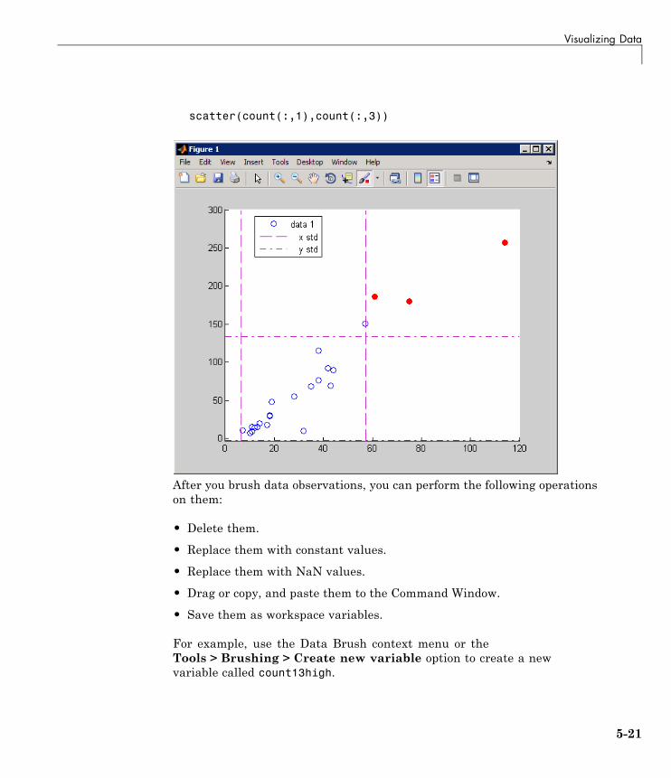
Visualizing Data
scatter(count(:,1),count(:,3))
After you brush data observations, you can perform the following operationson them:
• Delete them.
• Replace them with constant values.
• Replace them with NaN values.
• Drag or copy, and paste them to the Command Window.
• Save them as workspace variables.
For example, use the Data Brush context menu or theTools > Brushing > Create new variable option to create a newvariable called count13high.
5-21
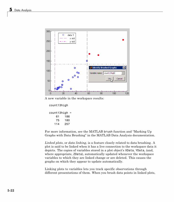
5 Data Analysis
A new variable in the workspace results:
count13high
count13high =61 18675 180
114 257
For more information, see the MATLAB brush function and “Marking UpGraphs with Data Brushing” in the MATLAB Data Analysis documentation.
Linked plots, or data linking, is a feature closely related to data brushing. Aplot is said to be linked when it has a live connection to the workspace data itdepicts. The copies of variables stored in a plot object’s XData, YData, (and,where appropriate, ZData), automatically updated whenever the workspacevariables to which they are linked change or are deleted. This causes thegraphs on which they appear to update automatically.
Linking plots to variables lets you track specific observations throughdifferent presentations of them. When you brush data points in linked plots,
5-22
Visualizing Data
brushing one graph highlights the same observations in every graph that islinked to the same variables.
Data linking establishes immediate, two-way communication betweenfigures and workspace variables, in the same way that the Variable Editorcommunicates with workspace variables. You create links by activating the
Data Linking tool on a figure’s toolbar. Activating this tool causes theLinked Plot information bar, displayed in the next figure, to appear at the topof the plot (possibly obscuring its title). You can dismiss the bar (shown inthe following figure) without unlinking the plot; it does not print and is notsaved with the figure.
The following two graphs depict scatter plot displays of linked data afterbrushing some observations on the left graph. The common variable, countcarries the brush marks to the right figure. Even though the right graphis not in data brushing mode, it displays brush marks because it is linkedto its variables.
figurescatter(count(:,1),count(:,2))xlabel ('count(:,1)')ylabel ('count(:,2)')figurescatter(count(:,3),count(:,2))xlabel ('count(:,3)')ylabel ('count(:,2)')
5-23

5 Data Analysis
The right plot shows that the brushed observations are more linearly relatedthan in the left plot.
Brushed data observations appear highlighted in the brushing color when youdisplay those variables in the Variable Editor, as you can see here:
openvar count
5-24

Visualizing Data
In the Variable Editor, you can alter any values of linked plot data, and thegraphs will reflect your edits. To brush data observation from the Variable
Editor, click its Brushing Tool button. If the variable you brush iscurrently depicted in a linked plot, the observations you brush highlight inthe plot as well as in the Variable Editor. When you brush a variable that isa column in a matrix, the other columns in that row are also brushed. Thatis, you can brush individual observations in a row or column vector, but all
5-25
5 Data Analysis
columns in a matrix highlight in any row you brush, not just the observationsyou click.
For more information, see the linkdata function, “Making Graphs Responsivewith Data Linking” in the MATLAB Data Analysis documentation, and“Viewing and Editing Values in the Current Workspace” in the MATLABDesktop Environment documentation.
5-26
Modeling Data
Modeling Data
In this section...
“Overview” on page 5-27
“Polynomial Regression” on page 5-27
“General Linear Regression” on page 5-28
OverviewParametric models translate an understanding of data relationships intoanalytic tools with predictive power. Polynomial and sinusoidal models aresimple choices for the up and down trends in the traffic data.
Note This section continues the data analysis from “Visualizing Data” onpage 5-14.
Polynomial RegressionUse the polyfit function to estimate coefficients of polynomial models, thenuse the polyval function to evaluate the model at arbitrary values of thepredictor.
The following code fits the traffic data at the third intersection with apolynomial model of degree six:
load count.datc3 = count(:,3); % Data at intersection 3tdata = (1:24)';p_coeffs = polyfit(tdata,c3,6);
figureplot(c3,'o-')hold ontfit = (1:0.01:24)';yfit = polyval(p_coeffs,tfit);plot(tfit,yfit,'r-','LineWidth',2)legend('Data','Polynomial Fit','Location','NW')
5-27
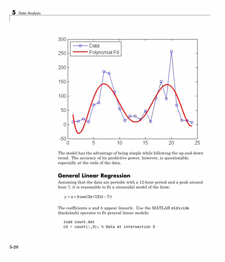
5 Data Analysis
The model has the advantage of being simple while following the up-and-downtrend. The accuracy of its predictive power, however, is questionable,especially at the ends of the data.
General Linear RegressionAssuming that the data are periodic with a 12-hour period and a peak aroundhour 7, it is reasonable to fit a sinusoidal model of the form:
y a b t= + −cos(( / )( ))2 12 7π
The coefficients a and b appear linearly. Use the MATLAB mldivide(backslash) operator to fit general linear models:
load count.datc3 = count(:,3); % Data at intersection 3
5-28
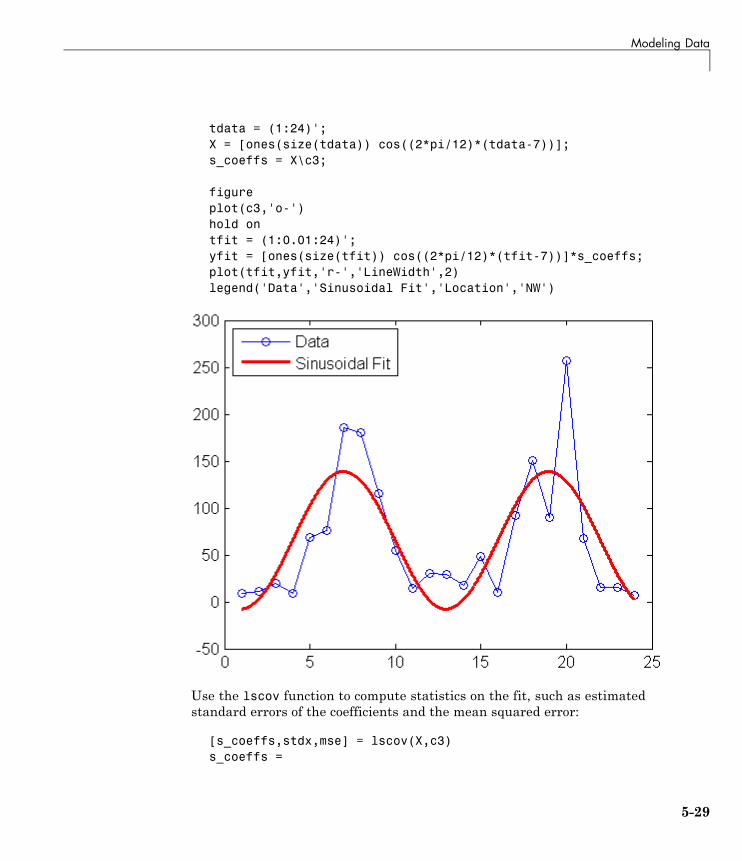
Modeling Data
tdata = (1:24)';X = [ones(size(tdata)) cos((2*pi/12)*(tdata-7))];s_coeffs = X\c3;
figureplot(c3,'o-')hold ontfit = (1:0.01:24)';yfit = [ones(size(tfit)) cos((2*pi/12)*(tfit-7))]*s_coeffs;plot(tfit,yfit,'r-','LineWidth',2)legend('Data','Sinusoidal Fit','Location','NW')
Use the lscov function to compute statistics on the fit, such as estimatedstandard errors of the coefficients and the mean squared error:
[s_coeffs,stdx,mse] = lscov(X,c3)s_coeffs =
5-29
5 Data Analysis
65.583373.2819
stdx =8.9185
12.6127mse =
1.9090e+003
Check the assumption of a 12-hour period in the data with a periodogram,computed using the fft function:
Fs = 1; % Sample frequency (per hour)n = length(c3); % Window lengthY = fft(c3); % DFT of dataf = (0:n-1)*(Fs/n); % Frequency rangeP = Y.*conj(Y)/n; % Power of the DFT
figureplot(f,P)xlabel('Frequency')ylabel('Power')
predicted_f = 1/12predicted_f =
0.0833
5-30
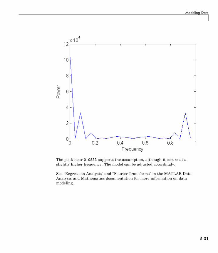
Modeling Data
The peak near 0.0833 supports the assumption, although it occurs at aslightly higher frequency. The model can be adjusted accordingly.
See “Regression Analysis” and “Fourier Transforms” in the MATLAB DataAnalysis and Mathematics documentation for more information on datamodeling.
5-31

5 Data Analysis
5-32
6
Creating Graphical UserInterfaces
• “What Is GUIDE?” on page 6-2
• “Laying Out a GUI” on page 6-3
• “Programming a GUI” on page 6-7
6 Creating Graphical User Interfaces
What Is GUIDE?GUIDE, the MATLAB graphical user interface development environment,provides a set of tools for creating graphical user interfaces (GUIs). Thesetools greatly simplify the process of designing and building GUIs. You can usethe GUIDE tools to perform the following tasks:
• Lay out the GUI.
Using the GUIDE Layout Editor, you can lay out a GUI easily by clickingand dragging GUI components—such as panels, buttons, text fields,sliders, menus, and so on—into the layout area. GUIDE stores the GUIlayout in a FIG-file.
• Program the GUI.
“GUIDE automatically generates a MATLAB program file that controlshow the GUI operates. The code in that file initializes the GUI andincludes function templates for the most commonly used callbacks foreach component—the commands that execute when a user clicks a GUIcomponent. Using the MATLAB editor, you can add code to the callbacksto perform the functions you want.
Note You can also create GUIs without GUIDE, by writing MATLAB code.For information on how to get started, see “How to Create a Simple GUIProgrammatically” in the MATLAB Creating Graphical User interfacesdocumentation.
6-2

Laying Out a GUI
Laying Out a GUI
In this section...
“Starting GUIDE” on page 6-3
“The Layout Editor” on page 6-4
Starting GUIDEStart GUIDE by typing guide at the MATLAB command prompt. Thiscommand displays the GUIDE Quick Start dialog box, as shown in thefollowing figure.
From the GUIDE Quick Start dialog box, you can perform the following tasks:
• Create a new GUI from one of the GUIDE templates—prebuilt GUIs thatyou can modify for your own purposes.
• Open an existing GUI.
6-3
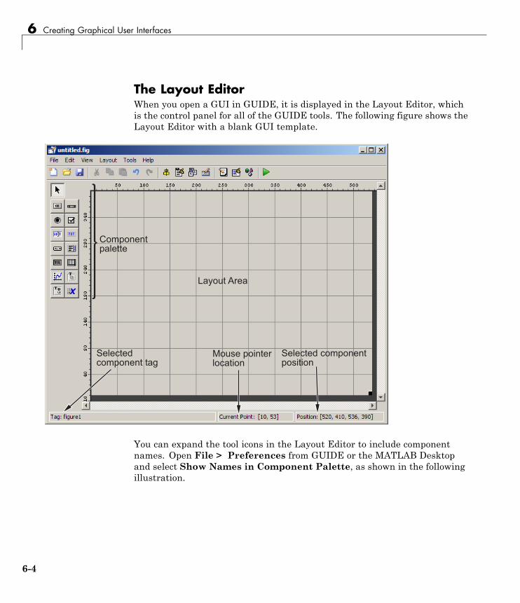
6 Creating Graphical User Interfaces
The Layout EditorWhen you open a GUI in GUIDE, it is displayed in the Layout Editor, whichis the control panel for all of the GUIDE tools. The following figure shows theLayout Editor with a blank GUI template.
$���������������
�� ��������
(�����������������
��������������������
(�����������������������
You can expand the tool icons in the Layout Editor to include componentnames. Open File > Preferences from GUIDE or the MATLAB Desktopand select Show Names in Component Palette, as shown in the followingillustration.
6-4
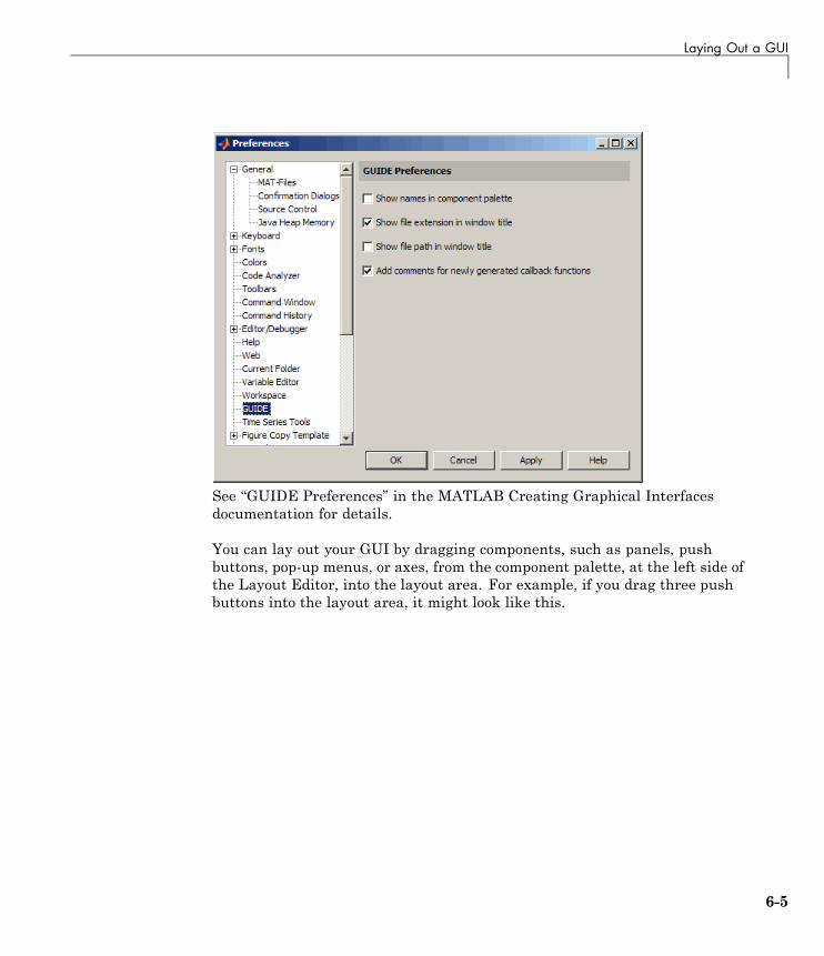
Laying Out a GUI
See “GUIDE Preferences” in the MATLAB Creating Graphical Interfacesdocumentation for details.
You can lay out your GUI by dragging components, such as panels, pushbuttons, pop-up menus, or axes, from the component palette, at the left side ofthe Layout Editor, into the layout area. For example, if you drag three pushbuttons into the layout area, it might look like this.
6-5
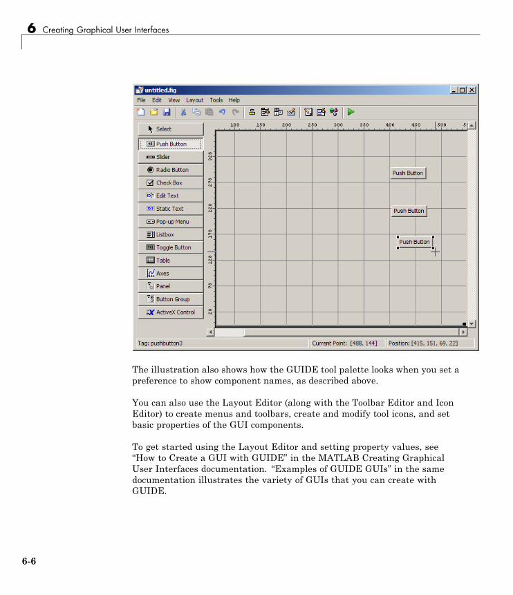
6 Creating Graphical User Interfaces
The illustration also shows how the GUIDE tool palette looks when you set apreference to show component names, as described above.
You can also use the Layout Editor (along with the Toolbar Editor and IconEditor) to create menus and toolbars, create and modify tool icons, and setbasic properties of the GUI components.
To get started using the Layout Editor and setting property values, see“How to Create a GUI with GUIDE” in the MATLAB Creating GraphicalUser Interfaces documentation. “Examples of GUIDE GUIs” in the samedocumentation illustrates the variety of GUIs that you can create withGUIDE.
6-6
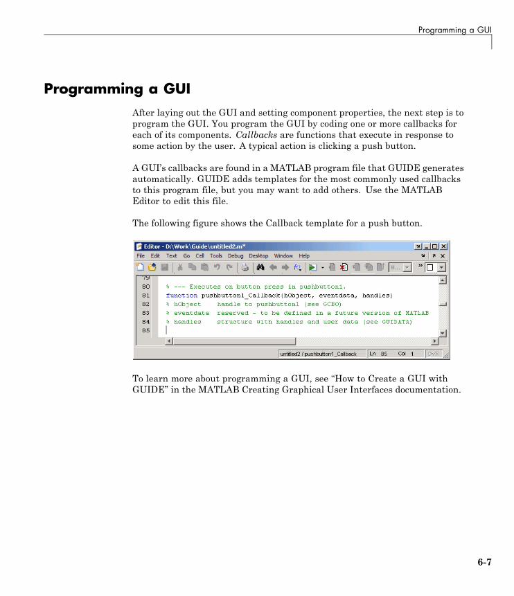
Programming a GUI
Programming a GUIAfter laying out the GUI and setting component properties, the next step is toprogram the GUI. You program the GUI by coding one or more callbacks foreach of its components. Callbacks are functions that execute in response tosome action by the user. A typical action is clicking a push button.
A GUI’s callbacks are found in a MATLAB program file that GUIDE generatesautomatically. GUIDE adds templates for the most commonly used callbacksto this program file, but you may want to add others. Use the MATLABEditor to edit this file.
The following figure shows the Callback template for a push button.
To learn more about programming a GUI, see “How to Create a GUI withGUIDE” in the MATLAB Creating Graphical User Interfaces documentation.
6-7

6 Creating Graphical User Interfaces
6-8
7
Desktop Tools andDevelopment Environment
If you have an active Internet connection, you can watch the Working inThe Development Environment video demo for an overview of the majorfunctionality.
• “Desktop Overview” on page 7-2
• “Command Window and Command History” on page 7-5
• “Getting Help” on page 7-7
• “Workspace Browser and Variable Editor” on page 7-20
• “Managing Files in MATLAB” on page 7-23
• “Finding and Getting Files Created by Other Users — File Exchange” onpage 7-27
• “Editor” on page 7-29
• “Improving and Tuning Your MATLAB Programs” on page 7-39
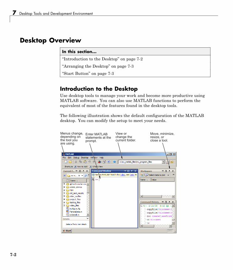
7 Desktop Tools and Development Environment
Desktop Overview
In this section...
“Introduction to the Desktop” on page 7-2
“Arranging the Desktop” on page 7-3
“Start Button” on page 7-3
Introduction to the DesktopUse desktop tools to manage your work and become more productive usingMATLAB software. You can also use MATLAB functions to perform theequivalent of most of the features found in the desktop tools.
The following illustration shows the default configuration of the MATLABdesktop. You can modify the setup to meet your needs.
��������� ������������������
�������������������������������������
�����������������������������������
�������� ���������� ����������� ���������� �
7-2
Desktop Overview
For More Information For an overview of the desktop, watch the Workingin the Development Environment video demo. For complete details, see theMATLAB Desktop Tools and Development Environment documentation.
Arranging the DesktopThese are some common ways to customize the desktop:
• Show or hide desktop tools via the Desktop menu.
• Resize any tool by dragging one of its edges.
• Move a tool outside of the desktop by clicking the undock button in thetool’s title bar.
• Reposition a tool within the desktop by dragging its title bar to the newlocation. As you drag, a blue box indicates the new tool position until yourelease the mouse button. You can drag more than one tools to the sameposition, in which case they become the same size and their title barsbecome tabs. Access a tabbed tool by clicking the tab displaying its name.
• Maximize or minimize (temporarily hide) a tool within the desktop viathe Desktop menu.
• Change fonts, customize the toolbar, and access other options by usingFile > Preferences.
Start ButtonThe MATLAB Start button provides easy access to tools, demos, shortcuts,and documentation. Click the Start button to see the options.
7-3

7 Desktop Tools and Development Environment
For More Information See “Desktop” in the MATLAB Desktop Tools andDevelopment Environment documentation.
7-4
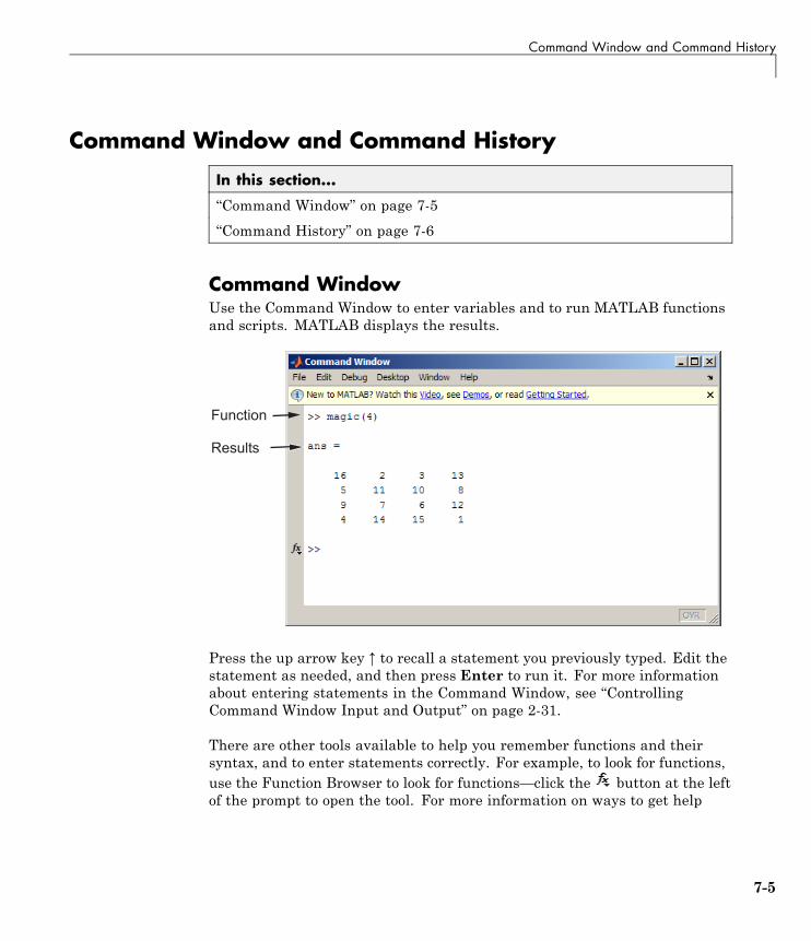
Command Window and Command History
Command Window and Command History
In this section...
“Command Window” on page 7-5
“Command History” on page 7-6
Command WindowUse the Command Window to enter variables and to run MATLAB functionsand scripts. MATLAB displays the results.
!������
,������
Press the up arrow key ↑ to recall a statement you previously typed. Edit thestatement as needed, and then press Enter to run it. For more informationabout entering statements in the Command Window, see “ControllingCommand Window Input and Output” on page 2-31.
There are other tools available to help you remember functions and theirsyntax, and to enter statements correctly. For example, to look for functions,use the Function Browser to look for functions—click the button at the leftof the prompt to open the tool. For more information on ways to get help
7-5
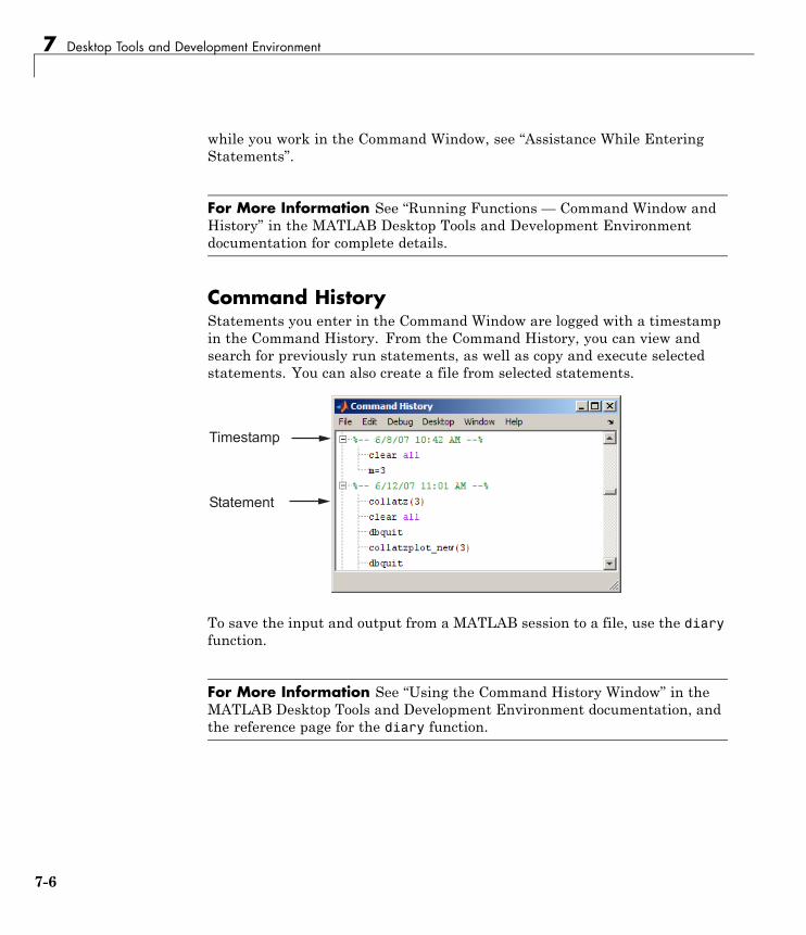
7 Desktop Tools and Development Environment
while you work in the Command Window, see “Assistance While EnteringStatements”.
For More Information See “Running Functions — Command Window andHistory” in the MATLAB Desktop Tools and Development Environmentdocumentation for complete details.
Command HistoryStatements you enter in the Command Window are logged with a timestampin the Command History. From the Command History, you can view andsearch for previously run statements, as well as copy and execute selectedstatements. You can also create a file from selected statements.
���������
(��������
To save the input and output from a MATLAB session to a file, use the diaryfunction.
For More Information See “Using the Command History Window” in theMATLAB Desktop Tools and Development Environment documentation, andthe reference page for the diary function.
7-6

Getting Help
Getting Help
In this section...
“Ways to Get Help” on page 7-7
“Accessing Documentation, Examples, and Demos Using the Help Browser”on page 7-9
“Searching for Documentation and Demos” on page 7-11
“Browsing for Documentation and Demos” on page 7-15
“Running Demos and Code in Examples” on page 7-16
Ways to Get HelpThere are different ways to get help, depending on your needs. The followingtable summarizes the main ways.
To... Try This More Information
Look for gettingstarted guides,code examples,demos, andmore.
In the Help browserContents pane, expandthe listing for a product.
“Browsing forDocumentation andDemos” on page 7-15
Findinformationabout any topic.
In the Help browser searchfield, type words youwant to look for in thedocumentation or demos.Then press Enter.
“Searching forDocumentation andDemos” on page 7-11
7-7
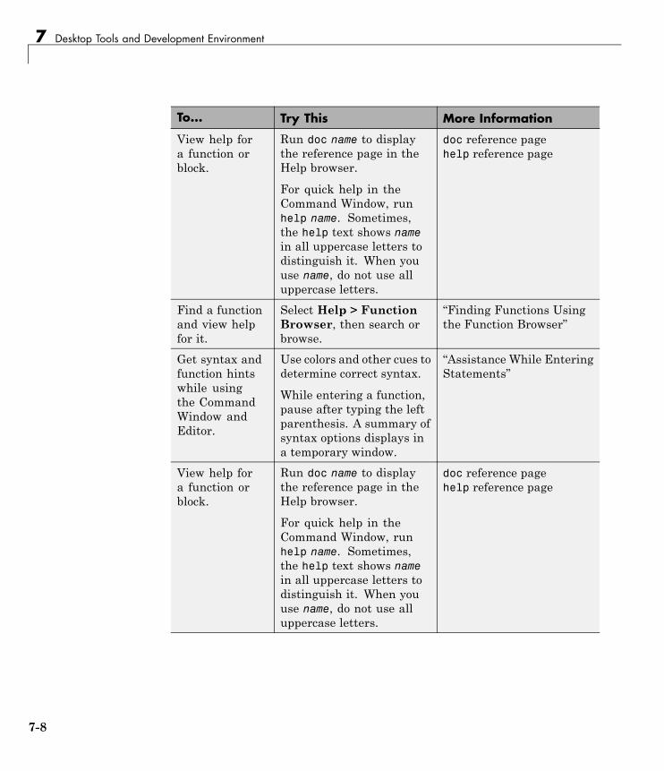
7 Desktop Tools and Development Environment
To... Try This More Information
View help fora function orblock.
Run doc name to displaythe reference page in theHelp browser.
For quick help in theCommand Window, runhelp name. Sometimes,the help text shows namein all uppercase letters todistinguish it. When youuse name, do not use alluppercase letters.
doc reference pagehelp reference page
Find a functionand view helpfor it.
Select Help > FunctionBrowser, then search orbrowse.
“Finding Functions Usingthe Function Browser”
Get syntax andfunction hintswhile usingthe CommandWindow andEditor.
Use colors and other cues todetermine correct syntax.
While entering a function,pause after typing the leftparenthesis. A summary ofsyntax options displays ina temporary window.
“Assistance While EnteringStatements”
View help fora function orblock.
Run doc name to displaythe reference page in theHelp browser.
For quick help in theCommand Window, runhelp name. Sometimes,the help text shows namein all uppercase letters todistinguish it. When youuse name, do not use alluppercase letters.
doc reference pagehelp reference page
7-8

Getting Help
To... Try This More Information
Get specific helpwhile using atool.
Use the context-sensitivehelp, which some toolsprovide. Access the helpusing standard methods,such as Help buttons andcontext menus.
See the documentation fora tool to learn about anyspecial context-sensitivehelp available.
Check codefor problemsand getrecommendationsforimprovements.
In the Editor, view M-Lintmessages.
“Preventing andIdentifying CodingProblems”
Accessing Documentation, Examples, and DemosUsing the Help BrowserThe Help browser is the main tool you use to view documentation, examplesin the documentation, and demos.
To open the Help browser, from any desktop tool, select Help > ProductHelp.
The Help browser shows Contents and Search Results in the left pane.When you select an item in the left pane, the right pane displays that page ofdocumentation or that demo.
Use the Help browser to find and view documentation and demos for allinstalled MathWorks products. To use documentation and demos for onlysome of the installed products, see “Specifying Which Documentation toDisplay”.
7-9
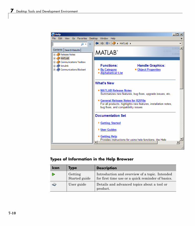
7 Desktop Tools and Development Environment
Types of Information in the Help Browser
Icon Type Description
GettingStarted guide
Introduction and overview of a topic. Intendedfor first time use or a quick reminder of basics.
User guide Details and advanced topics about a tool orproduct.
7-10
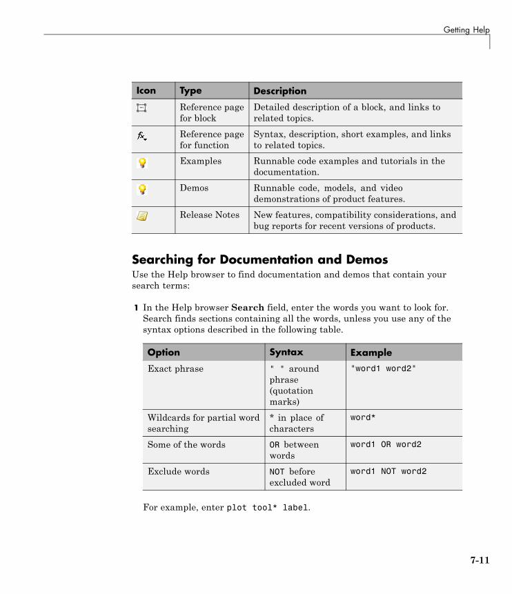
Getting Help
Icon Type Description
Reference pagefor block
Detailed description of a block, and links torelated topics.
Reference pagefor function
Syntax, description, short examples, and linksto related topics.
Examples Runnable code examples and tutorials in thedocumentation.
Demos Runnable code, models, and videodemonstrations of product features.
Release Notes New features, compatibility considerations, andbug reports for recent versions of products.
Searching for Documentation and DemosUse the Help browser to find documentation and demos that contain yoursearch terms:
1 In the Help browser Search field, enter the words you want to look for.Search finds sections containing all the words, unless you use any of thesyntax options described in the following table.
Option Syntax Example
Exact phrase " " aroundphrase(quotationmarks)
"word1 word2"
Wildcards for partial wordsearching
* in place ofcharacters
word*
Some of the words OR betweenwords
word1 OR word2
Exclude words NOT beforeexcluded word
word1 NOT word2
For example, enter plot tool* label.
7-11
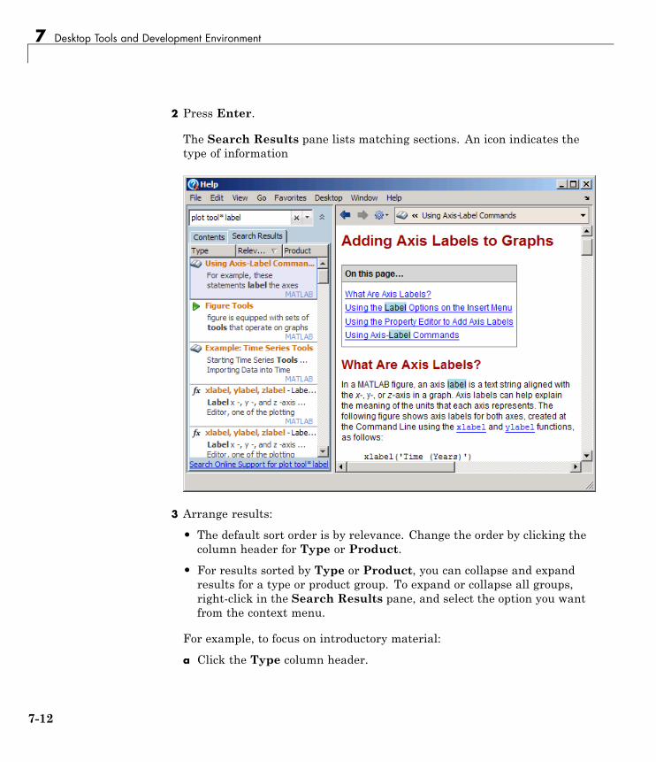
7 Desktop Tools and Development Environment
2 Press Enter.
The Search Results pane lists matching sections. An icon indicates thetype of information
3 Arrange results:
• The default sort order is by relevance. Change the order by clicking thecolumn header for Type or Product.
• For results sorted by Type or Product, you can collapse and expandresults for a type or product group. To expand or collapse all groups,right-click in the Search Results pane, and select the option you wantfrom the context menu.
For example, to focus on introductory material:
a Click the Type column header.
7-12
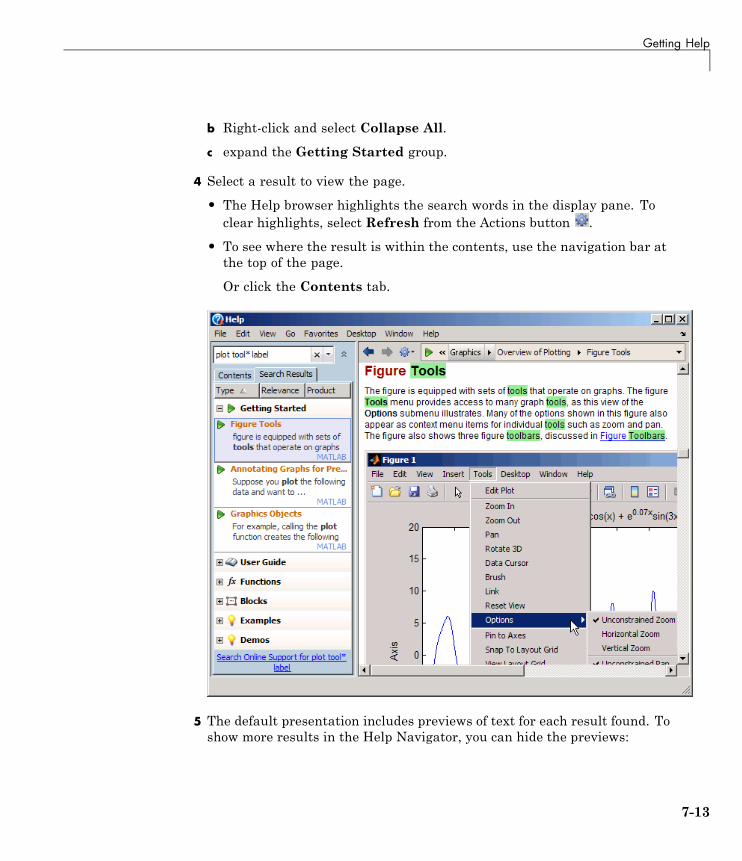
Getting Help
b Right-click and select Collapse All.
c expand the Getting Started group.
4 Select a result to view the page.
• The Help browser highlights the search words in the display pane. Toclear highlights, select Refresh from the Actions button .
• To see where the result is within the contents, use the navigation bar atthe top of the page.
Or click the Contents tab.
5 The default presentation includes previews of text for each result found. Toshow more results in the Help Navigator, you can hide the previews:
7-13
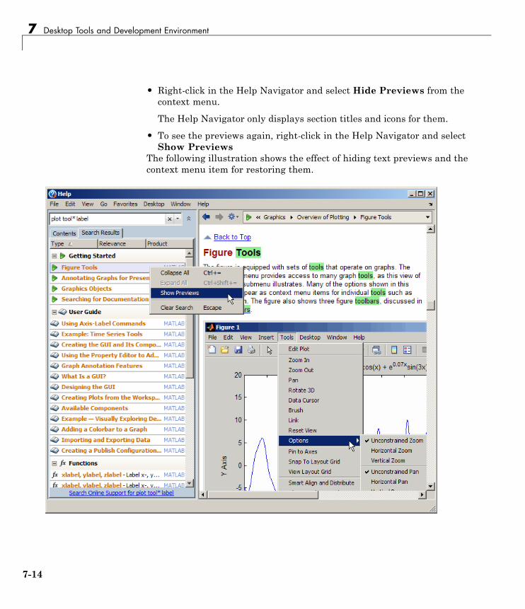
7 Desktop Tools and Development Environment
• Right-click in the Help Navigator and select Hide Previews from thecontext menu.
The Help Navigator only displays section titles and icons for them.
• To see the previews again, right-click in the Help Navigator and selectShow Previews
The following illustration shows the effect of hiding text previews and thecontext menu item for restoring them.
7-14
Getting Help
For more search options, see “Searching the Documentation” in the UserGuide.
Browsing for Documentation and DemosYou can find information by looking through a hierarchical view ofdocumentation and demos in the Help browser:
1 In the Help browser, click the Contents tab.
2 View the types of information available for a product by expanding theproduct in the Contents listing. For example, expand MATLAB.
3 View available items within an information type by expanding it. Forexample, within MATLAB, expand Demos, and then expand Graphics.
• Expand one item by clicking +. Or select the item and press the rightarrow key.
• Expand all items within the selected item by pressing the * key on thenumeric keypad.
4 To view an item in the display pane, select it. For example, within MATLAB> Demos > Graphics, select Square Wave from Sine Waves.
7-15
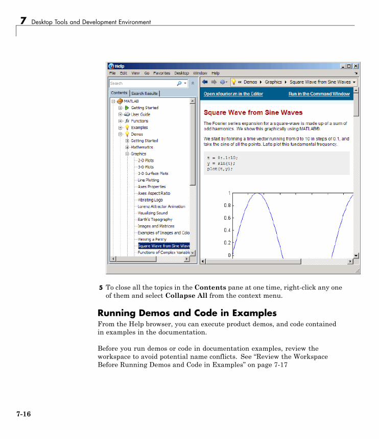
7 Desktop Tools and Development Environment
5 To close all the topics in the Contents pane at one time, right-click any oneof them and select Collapse All from the context menu.
Running Demos and Code in ExamplesFrom the Help browser, you can execute product demos, and code containedin examples in the documentation.
Before you run demos or code in documentation examples, review theworkspace to avoid potential name conflicts. See “Review the WorkspaceBefore Running Demos and Code in Examples” on page 7-17
7-16
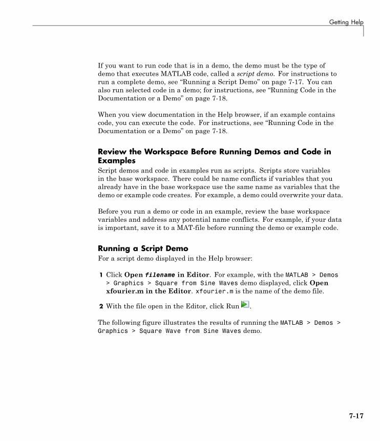
Getting Help
If you want to run code that is in a demo, the demo must be the type ofdemo that executes MATLAB code, called a script demo. For instructions torun a complete demo, see “Running a Script Demo” on page 7-17. You canalso run selected code in a demo; for instructions, see “Running Code in theDocumentation or a Demo” on page 7-18.
When you view documentation in the Help browser, if an example containscode, you can execute the code. For instructions, see “Running Code in theDocumentation or a Demo” on page 7-18.
Review the Workspace Before Running Demos and Code inExamplesScript demos and code in examples run as scripts. Scripts store variablesin the base workspace. There could be name conflicts if variables that youalready have in the base workspace use the same name as variables that thedemo or example code creates. For example, a demo could overwrite your data.
Before you run a demo or code in an example, review the base workspacevariables and address any potential name conflicts. For example, if your datais important, save it to a MAT-file before running the demo or example code.
Running a Script DemoFor a script demo displayed in the Help browser:
1 Click Open filename in Editor. For example, with the MATLAB > Demos> Graphics > Square from Sine Waves demo displayed, click Openxfourier.m in the Editor. xfourier.m is the name of the demo file.
2 With the file open in the Editor, click Run .
The following figure illustrates the results of running the MATLAB > Demos >Graphics > Square Wave from Sine Waves demo.
7-17
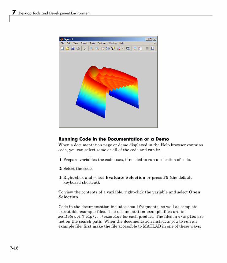
7 Desktop Tools and Development Environment
Running Code in the Documentation or a DemoWhen a documentation page or demo displayed in the Help browser containscode, you can select some or all of the code and run it:
1 Prepare variables the code uses, if needed to run a selection of code.
2 Select the code.
3 Right-click and select Evaluate Selection or press F9 (the defaultkeyboard shortcut).
To view the contents of a variable, right-click the variable and select OpenSelection.
Code in the documentation includes small fragments, as well as completeexecutable example files. The documentation example files are inmatlabroot/help/.../examples for each product. The files in examples arenot on the search path. When the documentation instructs you to run anexample file, first make the file accessible to MATLAB in one of these ways:
7-18
Getting Help
• Change the current folder to the folder containing the example file.
• Add to the search path the folder containing the example file.
• Copy the example file to another location that MATLAB can access.
For More Information There are additional options for getting help. See“Getting Help and Product Information”.
7-19
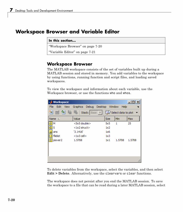
7 Desktop Tools and Development Environment
Workspace Browser and Variable Editor
In this section...
“Workspace Browser” on page 7-20
“Variable Editor” on page 7-21
Workspace BrowserThe MATLAB workspace consists of the set of variables built up during aMATLAB session and stored in memory. You add variables to the workspaceby using functions, running function and script files, and loading savedworkspaces.
To view the workspace and information about each variable, use theWorkspace browser, or use the functions who and whos.
To delete variables from the workspace, select the variables, and then selectEdit > Delete. Alternatively, use the clearvars or clear functions.
The workspace does not persist after you end the MATLAB session. To savethe workspace to a file that can be read during a later MATLAB session, select
7-20
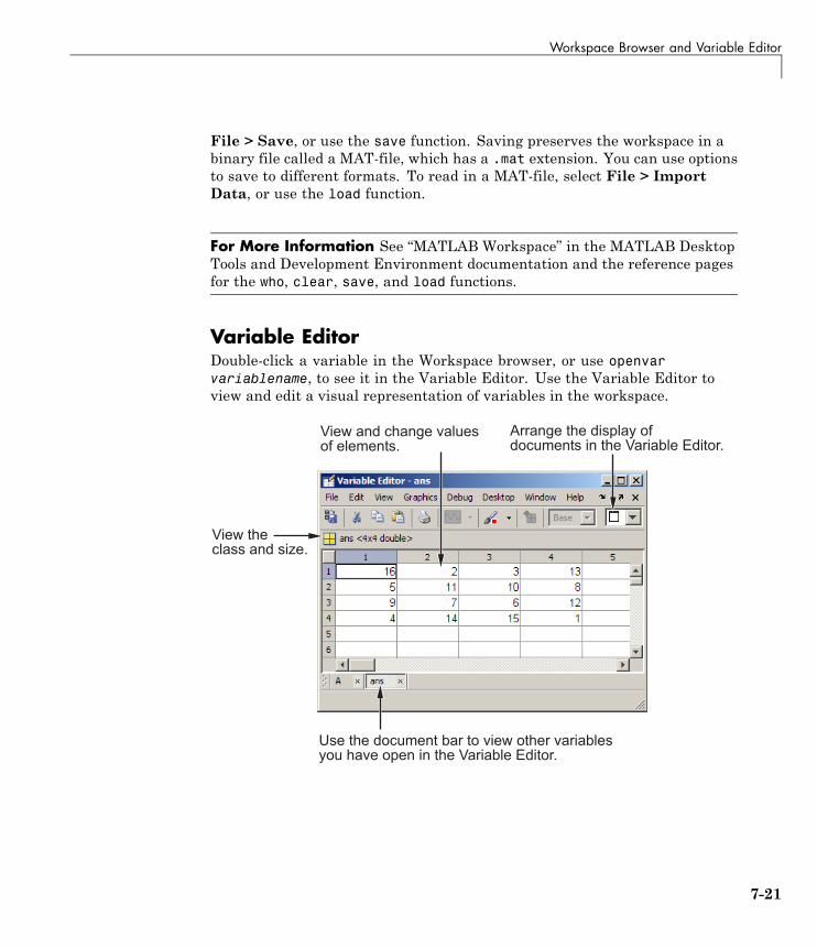
Workspace Browser and Variable Editor
File > Save, or use the save function. Saving preserves the workspace in abinary file called a MAT-file, which has a .mat extension. You can use optionsto save to different formats. To read in a MAT-file, select File > ImportData, or use the load function.
For More Information See “MATLAB Workspace” in the MATLAB DesktopTools and Development Environment documentation and the reference pagesfor the who, clear, save, and load functions.
Variable EditorDouble-click a variable in the Workspace browser, or use openvarvariablename, to see it in the Variable Editor. Use the Variable Editor toview and edit a visual representation of variables in the workspace.
-��������������#���������������������#��� �����������������������#����������
����������� ��������������������
����� ����������� �����������������������#����������
���������������������
7-21

7 Desktop Tools and Development Environment
For More Information See “Viewing and Editing Workspace Variableswith the Variable Editor” in the MATLAB Desktop Tools and DevelopmentEnvironment documentation and the reference page for the openvar function.
7-22
Managing Files in MATLAB®
Managing Files in MATLAB
In this section...
“How MATLAB Helps You Manage Files” on page 7-23
“Making Files Accessible to MATLAB” on page 7-23
“Using the Current Folder Browser to Manage Files” on page 7-24
“More Ways to Manage Files” on page 7-26
How MATLAB Helps You Manage FilesMATLAB provides tools and functions to help you:
• Find a file you want to view, change, or run
• Organize your files
• Ensure MATLAB can access a file so you can run or load it
Making Files Accessible to MATLABMATLAB limits where it looks for files so it can locate them more quickly.To run or get help for a MATLAB program file, or to load a MAT-file, thefile must be in one of these locations:
• MATLAB current folder
• A folder that is on the MATLAB search path
Similarly, files called by files you run also must be in one of these locations.
Special cases are:
• Private, class, and package folders
• When there are multiple files with the same name accessible to MATLAB
By default, files provided with MathWorks products are in folders on thesearch path. You do not have to do anything for MATLAB to access thefiles. These files are in matlabroot/toolbox. To determine the location ofmatlabroot, run the matlabroot function.
7-23
7 Desktop Tools and Development Environment
By default, the search path also includes a folder named MATLAB where youcan store files that you and other users create. To determine the location ofthe MATLAB folder, run the userpath function.
To access files in any other location, either:
• Make the folder containing the files be the current folder
• Add the folders containing the files to the search path.
Note Do not store files under matlabroot/toolbox, or you could experienceproblems.
Using the Current Folder Browser to Manage FilesThe Current Folder browser is a key tool for managing files.
Open the Current Folder browser by selecting Desktop > Current Folderfrom the MATLAB desktop.
7-24

Managing Files in MATLAB®
Use the Current Folder browser to:
• See the contents of the current folder.
• View and change the current folder using the address bar.
• Find files and folders using the search tool .
• Arrange information about files and folders using the View menu.
• Change files and folders, such as renaming or moving them.
7-25
7 Desktop Tools and Development Environment
• Run, open, get help for, and perform other actions on the selected file orfolder by right-clicking and using the context menu.
More Ways to Manage Files
• Change the search path using the Set Path dialog box. To open it, selectFile > Set Path.
• Find files and content within files across multiple folders using the FindFiles tool. To open the tool, select Edit > Find Files.
• View and change the current folder using the Current Folder field in thedesktop toolbar.
• Manage files programmatically using functions. See the function category,“Managing Files”.
For More Information See “Managing Files in MATLAB” in the MATLABDesktop Tools and Development Environment documentation
7-26
Finding and Getting Files Created by Other Users — File Exchange
Finding and Getting Files Created by Other Users — FileExchange
Use files created by other MATLAB users to save you time and provide youwith new ideas for your own work.
Users who want to share their files submit them to the File Exchangerepository at the MathWorks Web site.
You can then:
• Access the repository using the File Exchange desktop tool.
• Log in using your MathWorks Account.
• Use the tool to find, view details about, and download files to use.
7-27
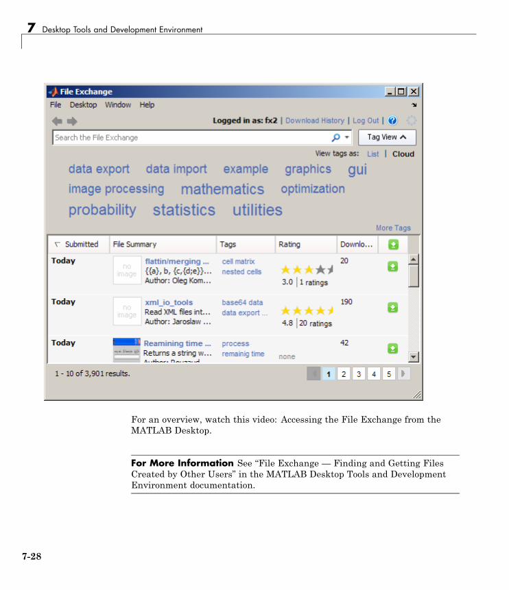
7 Desktop Tools and Development Environment
For an overview, watch this video: Accessing the File Exchange from theMATLAB Desktop.
For More Information See “File Exchange — Finding and Getting FilesCreated by Other Users” in the MATLAB Desktop Tools and DevelopmentEnvironment documentation.
7-28
Editor
Editor
In this section...
“Editing MATLAB Code Files” on page 7-29
“Identifying Problems and Areas for Improvement” on page 7-31
“Publishing MATLAB Code Files” on page 7-33
Editing MATLAB Code FilesUse the Editor to create and debug programs you write for running MATLABfunctions. The Editor provides a graphical user interface for text editingand debugging MATLAB code.
To create or edit a file select File > New or File > Open, or use the editfunction.
The following image shows the Editor with two documents, collatzall.m andcollatz.m open. Notice the following:
• Colors highlight various MATLAB language elements — blue for keywords,green for comments.
• The code analysis message bar contains an orange box and bar, indicatingthere are areas for improvement in the code.
Other Editor features are described in the image.
7-29

7 Desktop Tools and Development Environment
�������%������������������� ����������
��������#���$�������� ������ ��#�
.�������#�����������/��%���������������������
(������#�����������������������������������#��������������������
You can use any text editor to create files, such as Emacs. UseEditor/Debugger preferences (accessible from the desktop by selectingFile > Preferences > Editor/Debugger) to specify your default editor. Ifyou use another editor, you still can use the MATLAB Editor for debugging,or you can use debugging functions, such as dbstop, which sets a breakpoint.
To view the contents of a file, you can display the contents in the CommandWindow using the type function.
Use code analysis to help you identify problems and potential improvementsin your code. For details, see “Improving and Tuning Your MATLABPrograms” on page 7-39.
7-30
Editor
You can evaluate your code in sections (called code cells). Also, you can publishyour code, including results, to popular output formats like HTML. For moreinformation, see “Evaluating Subsections of Files Using Code Cells” in theMATLAB Desktop Tools and Development Environment documentation.
For More Information See “Editing and Debugging MATLAB Code”, thefunction reference pages for edit, type, and the list of “Debugging Functions”functions.
Identifying Problems and Areas for ImprovementUse code analysis to help you write correct and efficient MATLAB code. Codeanalysis:
• Identifies areas for improvement by underlining code in orange
• Identifies errors by underlining code in red
• Provides short messages, called M-Lint messages, to describe all suspectedtrouble spots
• Provides extended M-Lint messages for many suspected trouble spots
• Provides automated fixes for many trouble spots
The following images show code with a message at line 23 and 24. TheDetails button in the first message indicates that an extended message isavailable for that first problem. To have MATLAB fix a problem for you, clickthe Fix button, if displayed.
7-31

7 Desktop Tools and Development Environment
When you click a Details button, the message extends and provides a detailedexplanation, a suggested action, and sometimes links to the documentation.
7-32
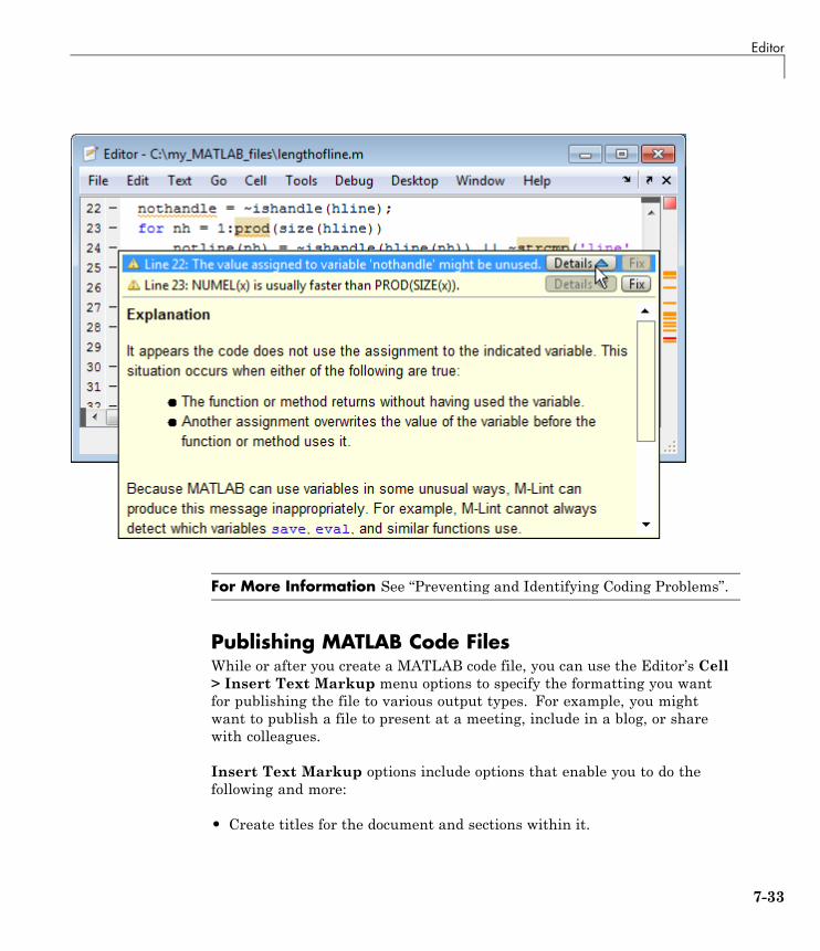
Editor
For More Information See “Preventing and Identifying Coding Problems”.
Publishing MATLAB Code FilesWhile or after you create a MATLAB code file, you can use the Editor’s Cell> Insert Text Markup menu options to specify the formatting you wantfor publishing the file to various output types. For example, you mightwant to publish a file to present at a meeting, include in a blog, or sharewith colleagues.
Insert Text Markup options include options that enable you to do thefollowing and more:
• Create titles for the document and sections within it.
7-33
7 Desktop Tools and Development Environment
• Specify the text format — bold, italic, monospaced, or hyperlinked
• Insert an image
• Format lists
7-34
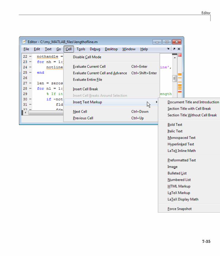
Editor
7-35
7 Desktop Tools and Development Environment
After adding text markup, click the Publish button on the Editor toolbar.By default, MATLAB software generates formatted HTML output andpresents the document in the MATLAB Web Browser.
7-36
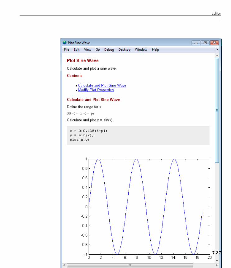
Editor
7-37

7 Desktop Tools and Development Environment
You can publish MATLAB code files to HTML, XML, LaTeX, and PDF. If yoursystem is a personal computer (PC), you also can publish files to MicrosoftWord and PowerPoint®.
For More Information See “Publishing MATLAB Code” in the MATLABDesktop Tools and Development Environment documentation, and thepublish reference page.
7-38
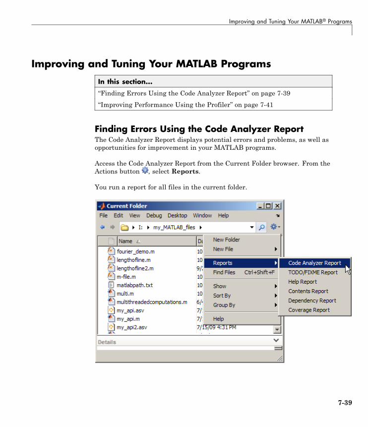
Improving and Tuning Your MATLAB® Programs
Improving and Tuning Your MATLAB Programs
In this section...
“Finding Errors Using the Code Analyzer Report” on page 7-39
“Improving Performance Using the Profiler” on page 7-41
Finding Errors Using the Code Analyzer ReportThe Code Analyzer Report displays potential errors and problems, as well asopportunities for improvement in your MATLAB programs.
Access the Code Analyzer Report from the Current Folder browser. From theActions button , select Reports.
You run a report for all files in the current folder.
7-39
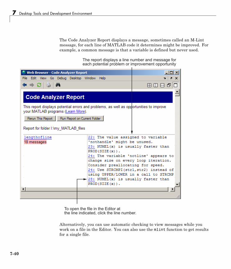
7 Desktop Tools and Development Environment
The Code Analyzer Report displays a message, sometimes called an M-Lintmessage, for each line of MATLAB code it determines might be improved. Forexample, a common message is that a variable is defined but never used.
���������������� ������������#������������ ���������������������#�����������������������������
���������������������������������������������������%������������#���
Alternatively, you can use automatic checking to view messages while youwork on a file in the Editor. You can also use the mlint function to get resultsfor a single file.
7-40
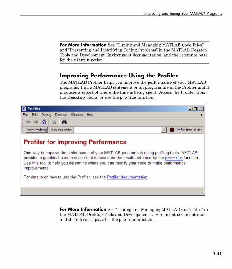
Improving and Tuning Your MATLAB® Programs
For More Information See “Tuning and Managing MATLAB Code Files”and “Preventing and Identifying Coding Problems” in the MATLAB DesktopTools and Development Environment documentation, and the reference pagefor the mlint function.
Improving Performance Using the ProfilerThe MATLAB Profiler helps you improve the performance of your MATLABprograms. Run a MATLAB statement or an program file in the Profiler and itproduces a report of where the time is being spent. Access the Profiler fromthe Desktop menu, or use the profile function.
For More Information See “Tuning and Managing MATLAB Code Files” inthe MATLAB Desktop Tools and Development Environment documentation,and the reference page for the profile function.
7-41
7 Desktop Tools and Development Environment
7-42

8
External Interfaces
Use MATLAB External Interfaces to connect MATLAB to programs, devicesand data. Application developers use external interfaces to integrateMATLAB functionality with their applications. External interfaces alsofacilitate data collection, such as from peripheral devices like an oscilloscopeor a remote network server.
• “Programming Interfaces” on page 8-2
• “Interface to .NET Framework” on page 8-4
• “Component Object Model Interface” on page 8-5
• “Web Services” on page 8-6
• “Serial Port Interface” on page 8-7
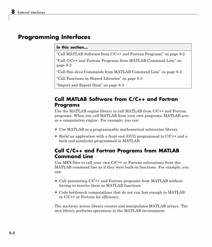
8 External Interfaces
Programming Interfaces
In this section...
“Call MATLAB Software from C/C++ and Fortran Programs” on page 8-2
“Call C/C++ and Fortran Programs from MATLAB Command Line” onpage 8-2
“Call Sun Java Commands from MATLAB Command Line” on page 8-3
“Call Functions in Shared Libraries” on page 8-3
“Import and Export Data” on page 8-3
Call MATLAB Software from C/C++ and FortranProgramsUse the MATLAB engine library to call MATLAB from C/C++ and Fortranprograms. When you call MATLAB from your own programs, MATLAB actsas a computation engine. For example, you can:
• Use MATLAB as a programmable mathematical subroutine library.
• Build an application with a front end (GUI) programmed in C/C++ and aback end (analysis) programmed in MATLAB.
Call C/C++ and Fortran Programs from MATLABCommand LineUse MEX-files to call your own C/C++ or Fortran subroutines from theMATLAB command line as if they were built-in functions. For example, youcan:
• Call preexisting C/C++ and Fortran programs from MATLAB withouthaving to rewrite them as MATLAB functions.
• Code bottleneck computations that do not run fast enough in MATLABin C/C++ or Fortran for efficiency.
The mxArray access library creates and manipulates MATLAB arrays. Themex library performs operations in the MATLAB environment.
8-2
Programming Interfaces
Call Sun Java Commands from MATLAB CommandLineEvery installation of MATLAB software includes Java Virtual Machine(JVM™) software. The JVM software allows you to use the MATLABinterpreter with Java commands and to create and access Java objects. Forexample, you can:
• Access Java API class packages that support I/O and networking.
• Access third-party Java classes.
• Construct Java objects in MATLAB.
• Call Java methods, using either Java or MATLAB syntax.
• Pass data between MATLAB variables and Java objects.
Call Functions in Shared LibrariesUse the MATLAB interface to shared libraries to interact with functionsin a dynamic link library (.dll) on Microsoft Windows platforms, a sharedobject file (.so) on UNIX and Linux® platforms, or a dynamic shared library(.dylib) on Apple Macintosh platforms based on Intel® technology.
MATLAB supports any shared library written in C, or in any language thatcan provide a C interface.
Import and Export DataMAT-files and the MAT-file access library provide a convenient mechanismfor moving MATLAB binary data between platforms, and for importing andexporting data to stand-alone MATLAB applications.
8-3
8 External Interfaces
Interface to .NET FrameworkMATLAB provides an interface to the Microsoft .NET Framework whichlets you leverage the capabilities of programming in .NET on the MicrosoftWindows platform.
8-4
Component Object Model Interface
Component Object Model InterfaceWith Microsoft COM (Component Object Model) tools and technologies, youcan integrate application-specific components from different vendors intoyour own applications. With COM, MATLAB software can include Microsoft®
ActiveX® controls or OLE server processes, or you can configure MATLAB asa computational server controlled by your client application programs.
For example, you can:
• Include ActiveX® components, like a calendar, in your MATLAB program.
• Access existing applications that expose objects via Automation, likeMicrosoft Excel.
• Access MATLAB as an Automation server from an application written inMicrosoft® Visual Basic® or C programming languages.
COM support in MATLAB is only available on the Microsoft Windowsplatform.
8-5
8 External Interfaces
Web ServicesWeb services are XML-based technologies for making remote procedure callsover a network. They enable communication between applications runningon disparate operating systems and development platforms. Web servicetechnologies available in the MATLAB software are:
• Simple Object Access Protocol (SOAP)
• Web Services Description Language (WSDL)
8-6
Serial Port Interface
Serial Port InterfaceThe MATLAB serial port interface provides direct access to peripheral devicesthat you connect to your computer’s serial port, such as modems, printers,and scientific instruments. For example, you can perform the following tasks:
• Configure serial port communications.
• Use serial port control pins.
• Write and read data.
• Use events and callbacks.
• Record information to disk.
8-7
8 External Interfaces
8-8
Index
IndexSymbols and Numerics: operator 2-82-D scatter plots
getting started 5-143-D scatter plots
getting started 5-16
Aalgorithms
vectorizing 4-31annotating plots 3-24ans function 2-5application program interface (API) 1-4array operators 2-25arrays 2-18
and matrices 2-25cell 4-11character 4-13columnwise organization 2-27deleting rows and columns 2-20elements 2-12generating with functions and operators 2-17listing contents 2-11loading from external data files 2-18multidimensional 4-9notation for elements 2-12preallocating 4-32structure 4-16variable names 2-11
arrow keys for editing commands 2-33aspect ratio of axes 3-67axes
managing 3-67visibility 3-68
axislabels 3-68titles 3-68
axis function 3-67
Bbit map 3-81break function 4-7browser
Help 7-9built-in functions
defined 2-14
Ccallbacks 6-7catch function 4-8cell arrays 4-11char function 4-15character arrays 4-13characteristic polynomial 2-24coefficient of determination
described 5-16colon operator 2-8colormap 3-74colors
lines for plotting 3-59Command History 7-6command line
editing 2-33Command Window 7-5complex numbers 2-13
plotting 3-62concatenation
defined 2-19of strings 4-14
constantsspecial 2-14
continue function 4-6continuing statements on multiple lines 2-33control keys for editing commands 2-33correlation coefficient
example using corrcoef 5-16covariance
example using cov 5-15
Index-1
Index
current folder 7-23Current Folder browser 7-24
Ddata analysis
getting started 5-1data source
for graphs 3-39debugging MATLAB code files 7-29deleting array elements 2-20demos 7-7
running from the Start button 7-3searching for 7-11
desktopfor MATLAB 1-7tools 7-1
determinant of matrix 2-22diag function 2-5distribution modeling
getting started 5-11documentation 7-7
searching 7-11
Eediting command lines 2-33Editor 7-29 7-33eigenvalue 2-23eigenvector 2-23elements of arrays 2-12entering matrices 2-4eval function 4-28examples 7-7executing MATLAB 1-7exiting MATLAB 1-8exporting graphs 3-53expressions
evaluating 4-28examples 2-15
using in MATLAB 2-11
Ffigure function 3-64figure tools 3-7figure windows 3-64
with multiple plots 3-65figures
adding and removing graphs 3-4files
debugging 7-29editing 7-29managing 7-23publishing 7-33
filtering datagetting started 5-6
find function 2-29finding object handles 3-93fliplr function 2-7floating-point numbers 2-12flow control 4-2folders
managing 7-23for loop 4-5format
of output display 2-31format function 2-31function files 4-20function functions 4-29function handles
defined 4-28using 4-30
function keyword 4-23function of two variables 3-72function program files
naming 4-22functions
built-in, defined 2-14defined 4-22
Index-2
Index
how to find 2-14running 7-5variable number of arguments 4-23
Gglobal variables 4-26graphical user interface
creating 6-1laying out 6-3programming 6-7
graphicsfiles 3-83Handle Graphics 3-85objects 3-86printing 3-82
grids 3-68GUIDE 6-1
HHandle Graphics 3-85
defined 1-3finding handles 3-93
Help browser 7-7 7-9searching 7-11
help functions 7-7highlighted search words 7-13hold function 3-63
Iimages 3-80imaginary numbers 2-12
Kkeys for editing in Command Window 2-33
Llegend
adding to plot 3-58legend function 3-58library
mathematical function 1-3lighting 3-76limits
axes 3-67line continuation 2-33line styles of plots 3-59linear regression
getting started 5-28load function 2-18loading arrays 2-18local variables 4-23log of functions used 7-6logical vectors 2-28
Mmagic function 2-9magic square 2-5markers 3-60MAT-file 3-80mathematical functions
library 1-3listing advanced 2-14listing elementary 2-14listing matrix 2-14
MATLABapplication program interface 1-4desktop 1-7executing 1-7exiting 1-8history 1-2language 1-3mathematical function library 1-3overview 1-2quitting 1-8
Index-3
Index
running 1-7shutting down 1-8starting 1-7
matrices 2-21creating 2-17entering 2-4
matrix 2-2antidiagonal 2-7determinant 2-22main diagonal 2-6multiplication 2-22singular 2-22swapping columns 2-10symmetric 2-21transpose 2-5
measures of locationgetting started 5-10
measures of scalegetting started 5-11
mesh plot 3-72missing data
getting started 5-3modeling data
getting started 5-27multidimensional arrays 4-9multiple data sets
plotting 3-58multiple plots per figure 3-65multivariate data
organizing 2-27
Nnumbers 2-12
complex 2-13floating-point 2-12
Oobject oriented programming 4-33
object properties 3-88objects
finding handles 3-93graphics 3-86
online help 7-7operators 2-13
colon 2-8outliers
getting started 5-4output
controlling format 2-31suppressing 2-32
overlaying plots 3-63
Ppath. See search pathperiodogram 5-30plot edit mode
description 3-24plot function 3-57Plot Selector tool
introduction to 3-15plots
editing 3-24plotting
adding legend 3-58adding plots 3-63basic 3-57complex data 3-62complex numbers 3-62contours 3-63editing 3-24functions 3-57line colors 3-59line styles 3-59lines and markers 3-60mesh and surface 3-72multiple data sets 3-58multiple plots 3-65
Index-4
Index
overview 3-2tools 3-10
polynomial regressiongetting started 5-27
PostScript 3-83preallocation 4-32preprocessing data
getting started 5-3present working directory. See current folderpresentation graphics 3-44principal components 5-17print function 3-82print preview
using 3-49printing
example 3-49graphics 3-82
Profiler 7-41program files
creating 4-20function 4-20scripts 4-20
Property Editorinterface 3-29
Property Inspector 3-26using 3-26
publishing code files 7-33
Qquitting MATLAB 1-8
Rreference pages 7-11release notes 7-11return function 4-8running
functions 7-5MATLAB 1-7
Sscalar expansion 2-28scatter plot arrays
getting started 5-18scientific notation 2-12script files 4-20scripts 4-21search path 7-23searching
Help browser 7-11semicolon to suppress output 2-32shutting down MATLAB 1-8singular matrix 2-22smoothing data
getting started 5-6special constants
infinity 2-15not-a-number 2-15
specialized graphs 3-64Start button 7-3starting MATLAB 1-7statements
continuing on multiple lines 2-33executing 4-28
stringsconcatenating 4-14
structures 4-16subplot function 3-65subscripting
with logical vectors 2-28subscripts 2-7sum function 2-5summarizing data
getting started 5-10suppressing output 2-32surface plot 3-72symmetric matrix 2-21
Index-5
Index
Ttext
entering in MATLAB 4-13TIFF 3-83title
figure 3-68toolboxes 1-2tools in the desktop 7-1transpose function 2-5try function 4-8
Uuserpath 7-23
VVariable Editor 7-21variables 2-11
global 4-26
local 4-23vectorization 4-31vectors 2-2
logical 2-28preallocating 4-32
visibility of axes 3-68visualizing data
getting started 5-14
Wwhile loop 4-6windows
in MATLAB 1-7windows for plotting 3-64wireframe
surface 3-72working directory. See current folderworkspace 7-20Workspace browser 7-20
Index-6