Getting started with Simulink The following tutorial gives a quick introduction to Simulink fore those that have not worked with Simulink before. It takes about 30 min to complete.

1 Introduction

What Is Simulink?Simulink is a software package for modeling, simulating, and analyzingdynamic systems. It supports linear and nonlinear systems, modeled incontinuous time, sampled time, or a hybrid of the two. Systems can also bemultirate, i.e., have different parts that are sampled or updated at differentrates.

Tool for SimulationSimulink encourages you to try things out. You can easily build models fromscratch, or take an existing model and add to it. You have instant access toall the analysis tools in MATLAB®, so you can take the results and analyzeand visualize them. A goal of Simulink is to give you a sense of the fun ofmodeling and simulation, through an environment that encourages you topose a question, model it, and see what happens.

Simulink is also practical. With thousands of engineers around the worldusing it to model and solve real problems, knowledge of this tool will serveyou well throughout your professional career.

Tool for Model-Based DesignWith Simulink, you can move beyond idealized linear models to explore morerealistic nonlinear models, factoring in friction, air resistance, gear slippage,hard stops, and the other things that describe real-world phenomena.Simulink turns your computer into a lab for modeling and analyzing systemsthat simply wouldn’t be possible or practical otherwise, whether the behaviorof an automotive clutch system, the flutter of an airplane wing, the dynamicsof a predator-prey model, or the effect of the monetary supply on the economy.Simulink provides numerous demos that model a wide variety of suchreal-world phenomena. For more information about accessing and executingthese demos, see Chapter 2, “Running a Model”.

For modeling, Simulink provides a graphical user interface (GUI) for buildingmodels as block diagrams, using click-and-drag mouse operations. Withthis interface, you can draw the models just as you would with pencil andpaper (or as most textbooks depict them). This is a far cry from previoussimulation packages that require you to formulate differential equationsand difference equations in a language or program. Simulink includes

1-2

What Is Simulink?

a comprehensive block library of sinks, sources, linear and nonlinearcomponents, and connectors. You can also customize and create your ownblocks. For information on creating your own blocks, see Writing S-Functionsin the online documentation.

Models are hierarchical, so you can build models using both top-downand bottom-up approaches. You can view the system at a high level, thendouble-click blocks to go down through the levels to see increasing levels ofmodel detail. This approach provides insight into how a model is organizedand how its parts interact.

After you define a model, you can simulate it, using a choice of integrationmethods, either from the Simulink menus or by entering commands in theMATLAB Command Window. The menus are particularly convenient forinteractive work, while the command-line approach is very useful for runninga batch of simulations (for example, if you are doing Monte Carlo simulationsor want to sweep a parameter across a range of values). Using scopes andother display blocks, you can see the simulation results while the simulationis running. In addition, you can change many parameters and see whathappens for “what if” exploration. The simulation results can be put in theMATLAB workspace for postprocessing and visualization.

Model analysis tools include linearization and trimming tools, which can beaccessed from the MATLAB command line, plus the many tools in MATLABand its application toolboxes. And because MATLAB and Simulink areintegrated, you can simulate, analyze, and revise your models in eitherenvironment at any point.

1-3

1 Introduction

Related ProductsThe MathWorks provides several products that are especially relevant tothe kinds of tasks you can perform with Simulink and that extend thecapabilities of Simulink. For information about these related products, seehttp://www.mathworks.com/products/simulink/related.html.

1-4

2

Running a Model

The following section gives you a quick introduction to running a Simulink®

model.

Running a Demo Model (p. 2-2) Example of how to run a Simulinkmodel.

About the Demo Model (p. 2-4) Explains how the model works.

Some Things to Try (p. 2-7) Suggests some model parameters tochange to see how they affect thesimulation.

What This Demo Illustrates (p. 2-7) Describes the common modelingand simulation tasks that this demoillustrates.

Other Useful Demos (p. 2-8) Shows how to find other demos thatillustrate key Simulink concepts andfeatures.

2 Running a Model

Running a Demo ModelAn interesting demo program provided with Simulink models thethermodynamics of a house. To run this demo, follow these steps:

1 Start MATLAB. See your MATLAB documentation if you’re not sure how todo this.

2 Run the demo model by typing thermo in the MATLAB Command Window.This command starts up Simulink and creates a model window thatcontains this model.

It also creates a scope window for the model. The Scope block displays twoplots labeled Indoor vs. Outdoor Temp and Heat Cost ($), respectively.

2-2

Running a Demo Model

3 To start the simulation, pull down the Simulation menu and choose theStart command (or, on Microsoft Windows, click the Start button onthe Simulink toolbar). As the simulation runs, the indoor and outdoortemperatures appear in the Indoor vs. Outdoor Temp plot as yellow andmagenta signals, respectively. The cumulative heating cost appears inthe Heat Cost ($) plot.

2-3

2 Running a Model

See Scope for further details about signal element colors.

4 To stop the simulation, choose the Stop command from the Simulationmenu (or click the Pause button on the toolbar). If you want to exploreother parts of the model, look over the suggestions in “Some Things toTry” on page 2-7.

5 When you’re finished running the simulation, close the model by choosingClose from the File menu.

About the Demo ModelThe demo models the thermodynamics of a house. The thermostat is set to 70degrees Fahrenheit and is affected by the outside temperature, which variesby applying a sine wave with amplitude of 15 degrees to a base temperatureof 50 degrees. This simulates daily temperature fluctuations.

2-4

About the Demo Model

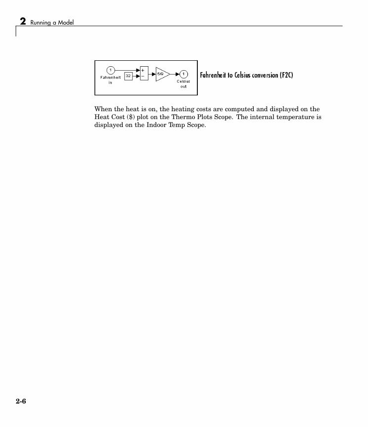
The model uses subsystems to simplify the model diagram and create reusablesystems. A subsystem is a group of blocks that is represented by a Subsystemblock. This model contains five subsystems: one named Thermostat, onenamed House, and three Temp Convert subsystems (two convert Fahrenheitto Celsius, one converts Celsius to Fahrenheit).

The internal and external temperatures are fed into the House subsystem,which updates the internal temperature. Double-click the House block to seethe underlying blocks in that subsystem.

The Thermostat subsystem models the operation of a thermostat, determiningwhen the heating system is turned on and off. Double-click the block to seethe underlying blocks in that subsystem.

Both the outside and inside temperatures are converted from Fahrenheit toCelsius by identical subsystems. Note that the conversion subsystems aremasks. Right-click the subsystem and select Look Under Mask to view thesubsystem (see “Creating Masked Subsystems” for further details).

2-5

2 Running a Model

When the heat is on, the heating costs are computed and displayed on theHeat Cost ($) plot on the Thermo Plots Scope. The internal temperature isdisplayed on the Indoor Temp Scope.

2-6

Some Things to Try

Some Things to TryHere are several things to try to see how the model responds to differentparameters:

• Each Scope block contains one or more signal display areas and controlsthat enable you to select the range of the signal displayed, zoom in on aportion of the signal, and perform other useful tasks. The horizontal axisrepresents time and the vertical axis represents the signal value.

• The Constant block labeled Set Point (at the top left of the model) setsthe desired internal temperature. Open this block and reset the valueto 80 degrees. Rerun the simulation to see how the indoor temperatureand heating costs change. Also, adjust the outside temperature (the AvgOutdoor Temp block) and rerun the simulation to see how it affects theindoor temperature.

• Adjust the daily temperature variation by opening the Sine Wave blocklabeled Daily Temp Variation and changing the Amplitude parameterand rerun the simulation.

What This Demo IllustratesThis demo illustrates several tasks commonly used when you are buildingmodels:

• Running the simulation involves specifying parameters and starting thesimulation with the Start command, described in “Running Simulations”.

• You can encapsulate complex groups of related blocks in a single block,called a subsystem. See “Creating Subsystems” for more information.

• You can customize the appearance of and design a dialog box for a blockby using the masking feature, described in detail in “Creating MaskedSubsystems”. The thermo model uses the masking feature to customize theappearance of all the Subsystem blocks that it contains.

• The Scope blocks display graphic output much as an actual oscilloscopedoes.

2-7

2 Running a Model

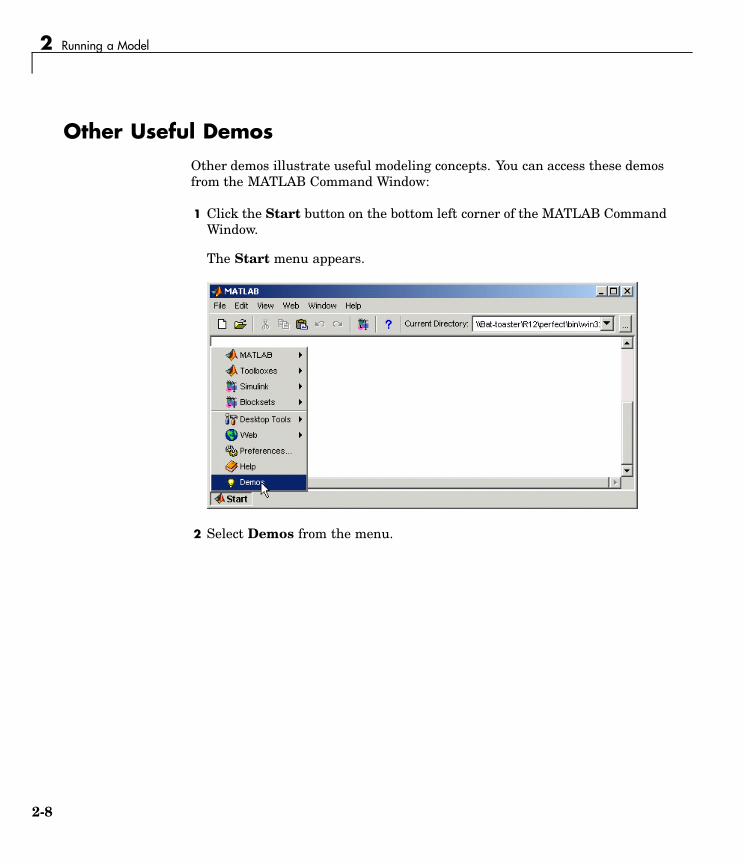
Other Useful DemosOther demos illustrate useful modeling concepts. You can access these demosfrom the MATLAB Command Window:

1 Click the Start button on the bottom left corner of the MATLAB CommandWindow.

The Start menu appears.

2 Select Demos from the menu.

2-8

Other Useful Demos

The MATLAB Help browser appears with the Demos pane selected.

3 Click the Simulink entry in the Demos pane.

The entry expands to show groups of Simulink demos. Use the browser tonavigate to demos of interest. The browser displays explanations of each demoand includes a link to the demo itself. Click on a demo link to start the demo.

2-9

2 Running a Model

2-10

3

Building a Model

The following sections show you to build a model of a simple dynamic system,using Simulink.

Model Example (p. 3-2) Example of how to build a Simulinkmodel.

Creating an Empty Model (p. 3-3) How to create an empty model.

Adding Blocks (p. 3-5) How to add blocks to a model.

Connecting the Blocks (p. 3-9) How to connect block outputs toblock inputs.

Configuring the Model (p. 3-12) How to select model configurationoptions.

Running the Model (p. 3-13) How to run a Simulink model.

3 Building a Model

Model ExampleThis example shows you how to build a model using many of themodel-building commands and actions you will use to build your own models.The instructions for building this model in this section are brief. All the tasksare described in more detail in the next chapter.

The model integrates a sine wave and displays the result along with the sinewave. The block diagram of the model looks like this.

3-2

Creating an Empty Model

Creating an Empty ModelTo create the model, first enter simulink in the MATLAB Command Window.On Microsoft Windows, the Simulink Library Browser appears.

3-3

Adding Blocks

Adding BlocksTo create this model, you need to copy blocks into the model from the followingSimulink block libraries:

• Sources library (the Sine Wave block)

• Sinks library (the Scope block)

• Continuous library (the Integrator block)

• Signal Routing library (the Mux block)

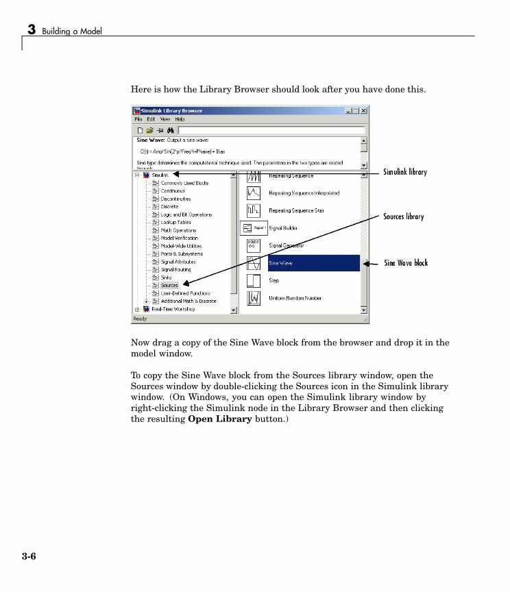
You can copy a Sine Wave block from the Sources library, using the LibraryBrowser (Windows only) or the Sources library window (UNIX, and Windows).

To copy the Sine Wave block from the Library Browser, first expand theLibrary Browser tree to display the blocks in the Sources library. Do this byclicking the Sources node to display the Sources library blocks. Finally, clickthe Sine Wave node to select the Sine Wave block.

3-5

3 Building a Model

Here is how the Library Browser should look after you have done this.

Now drag a copy of the Sine Wave block from the browser and drop it in themodel window.

To copy the Sine Wave block from the Sources library window, open theSources window by double-clicking the Sources icon in the Simulink librarywindow. (On Windows, you can open the Simulink library window byright-clicking the Simulink node in the Library Browser and then clickingthe resulting Open Library button.)

3-6

Adding Blocks

Simulink displays the Sources library window.

Now drag the Sine Wave block from the Sources window to your model window.

Copy the rest of the blocks in a similar manner from their respective librariesinto the model window. You can move a block from one place in the model

3-7

3 Building a Model

window to another by dragging the block. You can move a block a shortdistance by selecting the block, then pressing the arrow keys.

With all the blocks copied into the model window, the model should looksomething like this.

Notice that one or both sides of the blocks have angle brackets. The > symbolpointing out of a block is an output port; if the symbol points to a block, itis an input port.

3-8

Connecting the Blocks

Connecting the BlocksNow it’s time to connect the blocks. Connect the Sine Wave block to the topinput port of the Mux block. Position the pointer over the output port onthe right side of the Sine Wave block. Notice that the cursor shape changesto crosshairs.

Hold down the mouse button and move the cursor to the top input port ofthe Mux block.

Notice that the line is dashed while the mouse button is down and that thecursor shape changes to double-lined crosshairs as it approaches the Muxblock.

Now release the mouse button. The blocks are connected. You can alsoconnect the line to the block by releasing the mouse button while the pointeris over the block. If you do, the line is connected to the input port closest tothe cursor’s position.

If you look again at the model at the beginning of this section, you’ll noticethat most of the lines connect output ports of blocks to input ports of otherblocks. However, one line connects a line to the input port of anotherblock. This line, called a branch line, connects the Sine Wave output to the

3-9

3 Building a Model

Integrator block, and carries the same signal that passes from the Sine Waveblock to the Mux block.

Drawing a branch line is slightly different from drawing the line you justdrew. To weld a connection to an existing line, follow these steps:

1 First, position the pointer on the line between the Sine Wave and theMux block.

2 Press and hold down the Ctrl key (or click the right mouse button). Pressthe mouse button, then drag the pointer to the Integrator block’s input portor over the Integrator block itself.

3 Release the mouse button. Simulink draws a line between the startingpoint and the Integrator block’s input port.

3-10

Connecting the Blocks

Finish making block connections. When you’re done, your model should looksomething like this.

3-11

3 Building a Model

Configuring the ModelNow set up Simulink to run the simulation for 10 seconds. First, openthe Configuration Parameters dialog box by choosing ConfigurationParameters from the Simulation menu. On the dialog box that appears,notice that the Stop time is set to 10.0 (its default value).

Close the Configuration Parameters dialog box by clicking the OK button.Simulink applies the parameters and closes the dialog box.

3-12

Running the Model

Running the ModelNow double-click the Scope block to open its display window. Finally, chooseStart from the Simulation menu and watch the simulation output on theScope.

The simulation stops when it reaches the stop time specified in theConfiguration Parameters dialog box or when you choose Stop from theSimulation menu or click the Stop button on the model window’s toolbar(Windows only).

To save this model, choose Save from the File menu and enter a filename andlocation. That file contains the description of the model.

To terminate Simulink and MATLAB, choose Exit MATLAB (on a MicrosoftWindows system) or Quit MATLAB (on a UNIX system). You can also enterquit in the MATLAB Command Window. If you want to leave Simulink butnot terminate MATLAB, just close all Simulink windows.

This exercise shows you how to perform some commonly used model-buildingtasks. These and other tasks are described in more detail in “Creating aModel”.

3-13

Saving data to Matlab Workspace If not already open, open the Simulink Library Browser. Drag a copy of the To Workspace block from the browser and drop it in the model window

To Workspace block

Open the To Workspace block parameter by double clicking the block. Each Simulink block has a set of configurable parameters.

• Write a “good” name as Variable name. • Select the Save format pop up menu and select Array.

Close the Block Parameter window. Run the simulation again by choosing Start from the Simulation menu, or by pushing the black triangle in the graphical menu in the model window, or by typing Ctrl T. Now check the Matlab workspace and you will find a signal (array) with the name that you choose in the Block parameter. Plot the signal by executing, << plot(signalname) at the Matlab prompt. To plot the signal as a function of time instead as of only index, do the following. Chose Configure Parameters from the Simulation menu. Select the Data Import/Export page and verify that the Time box is checked and write a suitable name for the time signal, uncheck the Limit data points to last box.

Select the Time as output

Uncheck

Run the simulation again, check if the time is available in Matlab Workspace and plot the signal again, << plot(time,signal).

Grouping blocks The sine model is a very simple model which is easy to understand in terms of blocks and signal routing. For more complex files with many blocks and signals it is important to create a good model structure and signal naming. Copy the Integrator block by drag and drop with the right hand mouse button. Connect it as shown below, do not connect the output of the second integrator.

Select both integrator blocks by holding down the right mouse button and at the same time drawing a box around both blocks. In the Edit menu select Create Subsystem, reorganize the blocks such that the signal lines do not pass over each other or other blocks. Click on the Subsystem name and enter a name for the new subsystem. Open the subsystem by double clicking it. Rename the automatically created input port block and the two output port blocks, close the subsystem and connect a To Workspace block on each of the outputs of the subsystem. It should look something like the figure below. Simulate again and plot both signals.

Simulating and plotting directly from M-scripts To speed up development Simulink files can be simulated from the Matlab prompt or even better then from a M-script. The Matlab command sim is used to simulate a Simulink file, type << help sim at the the Matlab prompt for information how the command works.

• Open the Sine Wave block and write symbolic names instead of numerical values for amplitude and frequency.

• Create a new M-script by typing << edit at the Matlab prompt. • Write a M-script that simulates and plots the output of the first integrator for four

different amplitudes and four different frequencies. Combine the frequencies and amplitudes by using a double for loop in the M-script giving a total of 16 simulations.

• Execute the M-script by writing its name at the Matlab prompt. The result should look something like in the figure below

0 5 10 15 20 25 30−1

0

1

2

3

4

5

6

7

8

time

ampl

itude

sine wave signals