ggplot2and some stuff about R graphics and publication

level graphics

Kasper Daniel Hansen

Biostatistics Computing ClubMarch 3, 2010

1 / 39

Graphics

! Analysis Plotting in such a way that you understand the data better.Reaching the right conclusion is part of the purpose (Cleveland).

! Publication Plotting in such a way that others understand the databetter. You know the story you want to tell before you make theplot (Tufte).

Both authors are worth reading.(Tufte course in Philadelphia, 3/16, 200$ for fulltime students (includesfour books costing between 30$ and 35$ on Amazon). Worth it.)Useful R books: Murrell: R Graphics, Sarkar: Lattice: Multivariate DataVisualization with R, Wickham: ggplot2: Elegant graphics for dataanalysis.

2 / 39

Part I

The ggplot2 package

3 / 39

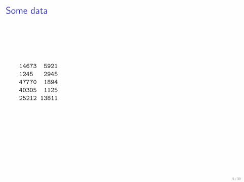
Some data

Some data

> library(ggplot2)> data(diamonds)> diamonds0 <- subset(diamonds, cut %in%+ c("Premium", "Very Good"))> dsmall <- diamonds0[sample(nrow(diamonds0),+ 100), ]> dsmall0 <- dsmall> head(dsmall[, -(8:10)])

carat cut color clarity depth table5022 0.91 Very Good F SI2 63.3 5414673 1.32 Premium I SI2 58.4 601245 0.79 Very Good H VS2 61.5 5547770 0.70 Very Good E SI2 63.5 5940305 0.40 Premium E VS1 61.8 5625212 1.51 Very Good G VS1 63.1 60

price5022 3746

4 / 39

Some data

14673 59211245 294547770 189440305 112525212 13811

5 / 39

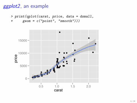
ggplot2 , an example

> print(qplot(carat, price, data = dsmall,+ geom = c("point", "smooth")))

carat

price

0

5000

10000

15000

●

●

●

●●

●

●

●

●●

●

●●

●

●

●

●

●

●

● ●

●

●●

●

●

●●

●

●

●

●

●●

●

●●

●

●

●

●

●

●

●

●

●

●

●

●

●

●

●

●

●

●

●

●

●

●

●

●

●

●

●

●

●

●●

●

●

●

●●

●

●

●●

●

●

●

●

●●

●

●

●●

●

●●

●●

●

●

●

●●

●

●

●

0.5 1.0 1.5 2.0

6 / 39

The Grammar of Graphics

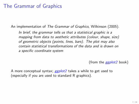
An implementation of The Grammar of Graphics, Wilkinson (2005).

In brief, the grammar tells us that a statistical graphic is amapping from data to aesthetic attributes (colour, shape, size)of geometric objects (points, lines, bars). The plot may alsocontain statistical transformations of the data and is drawn ona specific coordinate system

(from the ggplot2 book)

A more conceptual syntax; ggplot2 takes a while to get used to(especially if you are used to standard R graphics).

7 / 39

My perspective

! Produces very beautiful (but slow) graphics.

! Syntax takes a while to get used to.

! The package is very capable, but can be extremely hard tocustomize in ways that was not envisioned by the author.

! Very friendly email list (starting to be high volume).

! Help pages in R are often too brief and missing arguments; thewebsite (had.co.nz/ggplot2) is better.

! The book is invaluable.

! Worth investing time in.

! Code can be hard to access. Try

> help("geom_point")> geom_point> GeomPoint> GeomPoint$new> help("aes")

8 / 39

Key Components

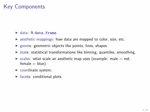
! data: A data.frame.

! aesthetic mappings: how data are mapped to color, size, etc.

! geoms: geometric objects like points, lines, shapes.

! stats: statistical transformations like binning, quantiles, smoothing.

! scales: what scale an aesthetic map uses (example: male = red,female = blue).

! coordinate system.

! facets: conditional plots.

9 / 39

Data, core functions

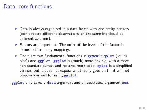
! Data is always organized in a data.frame with one entity per row(don’t record different observations on the same individual asdifferent columns).

! Factors are important. The order of the levels of the factor isimportant for many mappings.

! There are two fundamental functions in ggplot2 : qplot (“quickplot”) and ggplot. ggplot is (much) more flexible, with a morenon-standard syntax and requires more code. qplot is a simplifiedversion, but it does not expose what really goes on (= it will notprepare you well for using ggplot.

ggplot only takes a data argument and an aesthetics argument aes.

10 / 39

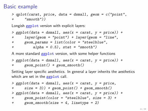
Basic example> qplot(carat, price, data = dsmall, geom = c("point",+ "smooth"))

Longish ggplot version with explicit layers:

> ggplot(data = dsmall, aes(x = carat, y = price)) ++ layer(geom = "point") + layer(geom = "line",+ geom_params = list(color = "steelblue",+ alpha = 0.5), stat = "smooth")

A more standard ggplot version, with some helper functions

> ggplot(data = dsmall, aes(x = carat, y = price)) ++ geom_point() + geom_smooth()

Setting layer specific aesthetics. In general a layer inherits the aestheticswhich are set in the ggplot call.

> ggplot(data = dsmall, aes(x = carat, y = price,+ size = 3)) + geom_point() + geom_smooth()> ggplot(data = dsmall, aes(x = carat, y = price)) ++ geom_point(color = "steelblue", size = 3) ++ geom_smooth(size = 4, linetype = 2)

11 / 39

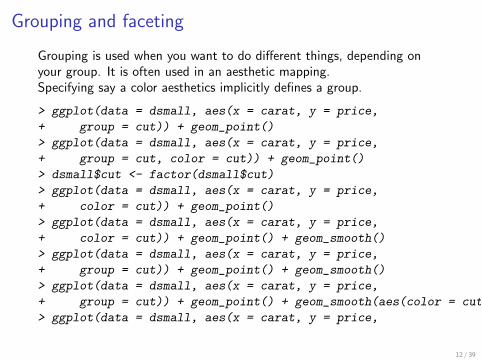
Grouping and faceting

Grouping is used when you want to do different things, depending onyour group. It is often used in an aesthetic mapping.Specifying say a color aesthetics implicitly defines a group.

> ggplot(data = dsmall, aes(x = carat, y = price,+ group = cut)) + geom_point()> ggplot(data = dsmall, aes(x = carat, y = price,+ group = cut, color = cut)) + geom_point()> dsmall$cut <- factor(dsmall$cut)> ggplot(data = dsmall, aes(x = carat, y = price,+ color = cut)) + geom_point()> ggplot(data = dsmall, aes(x = carat, y = price,+ color = cut)) + geom_point() + geom_smooth()> ggplot(data = dsmall, aes(x = carat, y = price,+ group = cut)) + geom_point() + geom_smooth()> ggplot(data = dsmall, aes(x = carat, y = price,+ group = cut)) + geom_point() + geom_smooth(aes(color = cut))> ggplot(data = dsmall, aes(x = carat, y = price,

12 / 39

Grouping and faceting

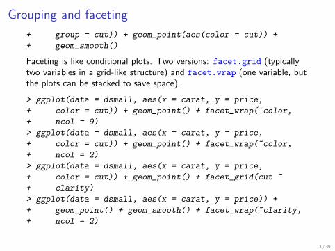
+ group = cut)) + geom_point(aes(color = cut)) ++ geom_smooth()

Faceting is like conditional plots. Two versions: facet.grid (typicallytwo variables in a grid-like structure) and facet.wrap (one variable, butthe plots can be stacked to save space).

> ggplot(data = dsmall, aes(x = carat, y = price,+ color = cut)) + geom_point() + facet_wrap(~color,+ ncol = 9)> ggplot(data = dsmall, aes(x = carat, y = price,+ color = cut)) + geom_point() + facet_wrap(~color,+ ncol = 2)> ggplot(data = dsmall, aes(x = carat, y = price,+ color = cut)) + geom_point() + facet_grid(cut ~+ clarity)> ggplot(data = dsmall, aes(x = carat, y = price)) ++ geom_point() + geom_smooth() + facet_wrap(~clarity,+ ncol = 2)

13 / 39

Annotation, arranging

! Labels: xlab(), ylab(), labs() (these are helper functions).

! Some things only make sense globally, there is opts() for that:opts(title = "Something"), opts(legend = "none")

! Two standard themes are included: theme_bw and theme_gray

! In order to do several plots in one figure (like par(mfrow =c(2,2))), you either need to learn grid or use arrange fromgridExtra from R-forge.

14 / 39

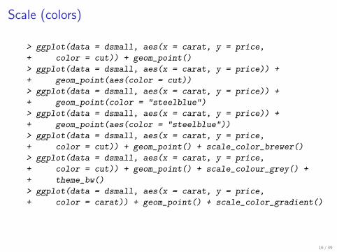
Scale (colors)

! Aesthetics maps data to a scale. The (by far) most confusingexample is color scales.

! One description: you can enumerate all the colors used in acomputer. This means they can be ordered. An ordering (possiblywith subsetting) is called a scale. You can think of a (color) scale asa map from [0, 1] to colorspace. Example: a grey scale and agradient.

! A three-level factor is mapped to color space by mapping the firstlevel to 0, the second to 1/2 and the third to 1. And then the scaleis used to map [0, 1] to color space.

! Mapping data values to a scale is different from setting a value.Several geoms can set aesthetics. Mapping happens through aes.

15 / 39

Scale (colors)

> ggplot(data = dsmall, aes(x = carat, y = price,+ color = cut)) + geom_point()> ggplot(data = dsmall, aes(x = carat, y = price)) ++ geom_point(aes(color = cut))> ggplot(data = dsmall, aes(x = carat, y = price)) ++ geom_point(color = "steelblue")> ggplot(data = dsmall, aes(x = carat, y = price)) ++ geom_point(aes(color = "steelblue"))> ggplot(data = dsmall, aes(x = carat, y = price,+ color = cut)) + geom_point() + scale_color_brewer()> ggplot(data = dsmall, aes(x = carat, y = price,+ color = cut)) + geom_point() + scale_colour_grey() ++ theme_bw()> ggplot(data = dsmall, aes(x = carat, y = price,+ color = carat)) + geom_point() + scale_color_gradient()

16 / 39

Limits

xlim, ylim are used all the time in base R graphics. In ggplot2 you canset limits through scale or a coordinate system. Using a scale discardsdata outside of the limits, using a coordinate system zooms the plot.Both approaches are slightly different from what base R does.

> testdat <- data.frame(x = 1:100, y = rnorm(100))> testdat[50, 2] <- 100> ggplot(testdat, aes(x = x, y = y)) + geom_line()> ggplot(testdat, aes(x = x, y = y)) + geom_line() ++ ylim(-3, 3)> ggplot(testdat, aes(x = x, y = y)) + geom_line() ++ coord_cartesian(ylim = c(-3, 3))> ggplot(testdat, aes(x = x, y = y)) + geom_line() ++ coord_cartesian(ylim = c(-3, 3)) ++ scale_y_continuous(breaks = c(-2,+ -1, 0, 1, 2))

17 / 39

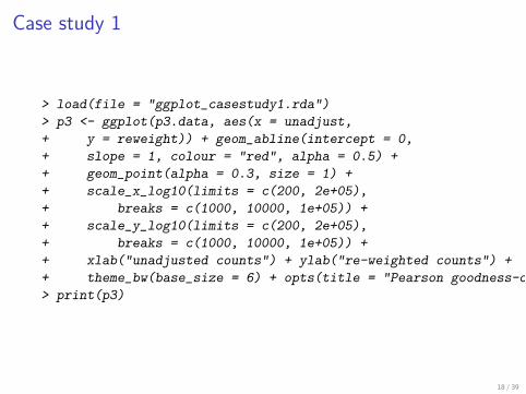
Case study 1

> load(file = "ggplot_casestudy1.rda")> p3 <- ggplot(p3.data, aes(x = unadjust,+ y = reweight)) + geom_abline(intercept = 0,+ slope = 1, colour = "red", alpha = 0.5) ++ geom_point(alpha = 0.3, size = 1) ++ scale_x_log10(limits = c(200, 2e+05),+ breaks = c(1000, 10000, 1e+05)) ++ scale_y_log10(limits = c(200, 2e+05),+ breaks = c(1000, 10000, 1e+05)) ++ xlab("unadjusted counts") + ylab("re-weighted counts") ++ theme_bw(base_size = 6) + opts(title = "Pearson goodness-of-fit")> print(p3)

18 / 39

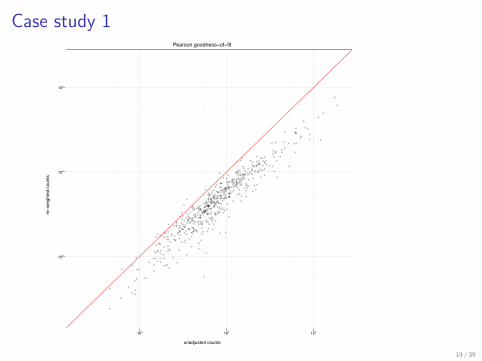
Case study 1Pearson goodness−of−fit

unadjusted counts

re−w

eigh

ted

coun

ts

103

104

105

103 104 105

19 / 39

Case study 1

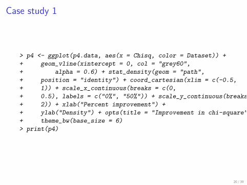
> p4 <- ggplot(p4.data, aes(x = Chisq, color = Dataset)) ++ geom_vline(xintercept = 0, col = "grey60",+ alpha = 0.6) + stat_density(geom = "path",+ position = "identity") + coord_cartesian(xlim = c(-0.5,+ 1)) + scale_x_continuous(breaks = c(0,+ 0.5), labels = c("0%", "50%")) + scale_y_continuous(breaks = c(0.5,+ 2)) + xlab("Percent improvement") ++ ylab("Density") + opts(title = "Improvement in chi-square") ++ theme_bw(base_size = 6)> print(p4)

20 / 39

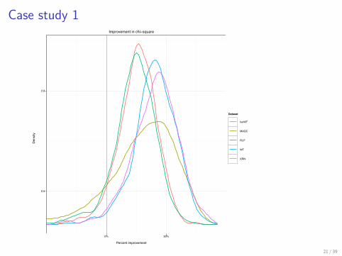
Case study 1Improvement in chi−square

Percent improvement

Dens

ity

0.5

2.0

0% 50%

Dataset

IsoWT

MAQC

RLP

WT

XRN

21 / 39

Case study 1

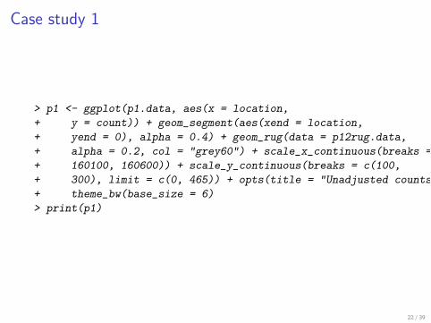
> p1 <- ggplot(p1.data, aes(x = location,+ y = count)) + geom_segment(aes(xend = location,+ yend = 0), alpha = 0.4) + geom_rug(data = p12rug.data,+ alpha = 0.2, col = "grey60") + scale_x_continuous(breaks = c(159600,+ 160100, 160600)) + scale_y_continuous(breaks = c(100,+ 300), limit = c(0, 465)) + opts(title = "Unadjusted counts") ++ theme_bw(base_size = 6)> print(p1)

22 / 39

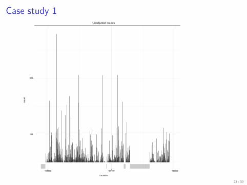
Case study 1Unadjusted counts

location

coun

t

100

300

159600 160100 160600

23 / 39

Case study 1

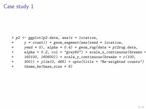
> p2 <- ggplot(p2.data, aes(x = location,+ y = count)) + geom_segment(aes(xend = location,+ yend = 0), alpha = 0.4) + geom_rug(data = p12rug.data,+ alpha = 0.2, col = "grey60") + scale_x_continuous(breaks = c(159600,+ 160100, 160600)) + scale_y_continuous(breaks = c(100,+ 300)) + ylim(0, 465) + opts(title = "Re-weighted counts") ++ theme_bw(base_size = 6)

24 / 39

Case study 1

> library(gridExtra)> grid.newpage()> print(arrange(p1, p3, p2, p4, nrow = 2))

frame[GRID.frame.892]

25 / 39

Case study 1Unadjusted counts

location

coun

t

100

300

159600 160100 160600

Pearson goodness−of−fit

unadjusted counts

re−w

eigh

ted

coun

ts

103

104

105

103 104 105

Re−weighted counts

location

coun

t

0

100

200

300

400

159600 160100 160600

Improvement in chi−square

Percent improvement

Dens

ity

0.5

2.0

0% 50%

Dataset

IsoWT

MAQC

RLP

WT

XRN

26 / 39

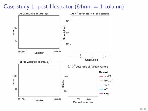
Case study 1, post Illustrator (84mm = 1 column)

Improvement in chi­square

Dataset

50%0%

IsoWT

MAQCRLP

WT

XRN

159,600

159,600 160,600

160,600Location

LocationPercent reduction

100

100

300

300 2.0

0.5

Unadjusted counts, c(l)

Re­weighted counts, cw(l)

105

104

103

105104103

goodness­of­fit comparison

UnadjustedRe­weighted

Density

(a)

(b)

(c)

(d)

Count

Count

goodness­of­fit improvement

27 / 39

Case study 2

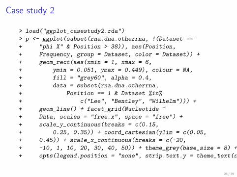
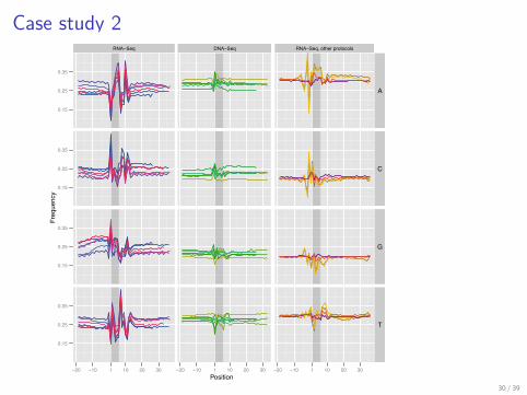
> load("ggplot_casestudy2.rda")> p <- ggplot(subset(rna.dna.otherrna, !(Dataset ==+ "phi X" & Position > 38)), aes(Position,+ Frequency, group = Dataset, color = Dataset)) ++ geom_rect(aes(xmin = 1, xmax = 6,+ ymin = 0.051, ymax = 0.449), colour = NA,+ fill = "grey60", alpha = 0.4,+ data = subset(rna.dna.otherrna,+ Position == 1 & Dataset %in%+ c("Lee", "Bentley", "Wilhelm"))) ++ geom_line() + facet_grid(Nucleotide ~+ Data, scales = "free_x", space = "free") ++ scale_y_continuous(breaks = c(0.15,+ 0.25, 0.35)) + coord_cartesian(ylim = c(0.05,+ 0.45)) + scale_x_continuous(breaks = c(-20,+ -10, 1, 10, 20, 30, 40, 50)) + theme_grey(base_size = 8) ++ opts(legend.position = "none", strip.text.y = theme_text(size = 8)) +

28 / 39

Case study 2

+ scale_colour_manual(values = colList)> print(p)

29 / 39

Case study 2

Position

Freq

uenc

y

0.15

0.25

0.35

0.15

0.25

0.35

0.15

0.25

0.35

0.15

0.25

0.35

RNA−Seq

−20 −10 1 10 20 30

DNA−Seq

−20 −10 1 10 20 30

RNA−Seq, other protocols

−20 −10 1 10 20 30

A

C

G

T

30 / 39

Case study 2, post Illustrator (178mm = 2 columns)

“hansen˙nar˙bias” — 2010/2/28 — 23:32 — page 3 — #3

! !

! !

Nucleic Acids Research, 2009, Vol. 37, No. 12 3

Fre

qu

en

cy

0.15

0.25

0.35

0.15

0.25

0.35

0.15

0.25

0.35

0.15

0.25

0.35

RNA-Seq

-20 -10 1 10 20 30

DNA-Seq

-20 -10 1 10 20 30

RNA-Seq, other protocols

-20 -10 1 10 20 30

A

C

G

T

Position

(a) (b) (c)

Bullard

Marioni

Mortazavi

Lee

Wang, brain

Wang, heart

Bentley

Wang, DNA

Chiang

Mikkelsen

Meissner Nagalakhsmi, RH

Nagalakhsmi, DT

Wilhelm

Bloom

RNA fragmentation,Ran. hex. priming

No fragmentation,Ran. hex. priming

DNA-Seq ChIP-Seq Oligo-dT priming,Nebulization (DNA)

Oligo-dT priming,DNase I (DNA)

Ribominus,Oligo-dT priming,Sonication (DNA)

Ran. hex. priming,DNase I (DNA)

phi X

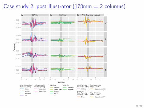
Figure 1. Nucleotide frequencies vs. position for stringently mapped reads. For each experiment, mapped reads were extended upstream of the 5’-start position,such that the first position of the actual read is 1 and positions 0 to -20 are obtained from the genome. The first hexamer of the read is shaded. Brief experimentalprotocols are indicated in the key. (a) RNA-Seq experiments conducted using priming with random hexamers, with and without RNA fragmentation. (b) DNAresequencing and ChIP-Seq experiments. (c) RNA-Seq experiments with alternative library preparation protocols, including priming with random hexamersfollowed by fragmentation using DNase I and priming with oligo(dT) followed by fragmentation using either DNase I, nebulization, or sonication.

This dependence of nucleotide frequency on position canoccur either because of a reproducible bias originating fromthe sequencing platform or because of a spatial bias of thereads across the transcriptome.In contrast to RNA-Seq, no strong distinctive pattern in

nucleotide frequencies is observed for DNA resequencingand ChIP-Seq experiments (10, 11, 12, 13, 14) (Figure 1band Supplementary Figure S2). This shows that the 5’nucleotide bias from RNA-Seq is not caused by the IlluminaGenome Analyzer DNA sequencing protocol, but rather byadditional steps in the RNA-Seq library preparation, namelyRNA extraction and reverse transcription into double-strandedcomplementary DNA (dscDNA). The standard protocoldescribed above was used in all experiments in Figure 1a,except for two experiments that omitted RNA fragmentation.Based on Figure 1c, we conclude that the pattern is

caused by the use of random hexamers to prime thereverse transcription of RNA into dscDNA. The figureshows a number of RNA-Seq experiments employingalternative library preparation protocols (15, 16, 17). Two

of these experiments used oligo(dT) priming followed byfragmentation of dscDNA using nebulization and sonication;both of these experiments show no dependence of thenucleotide frequencies on position. The other two experimentsemployed oligo(dT) priming and random hexamer priming,both followed by fragmentation of dscDNA using DNase I.The nucleotide frequencies for these latter two experimentshave similar patterns, but compared to the pattern of theRNA-Seq experiments of Figure 1a, this pattern is smallerin magnitude and extends upstream of the start position ofthe reads. Because the two different priming methods used inthese experiments result in the same pattern, we conclude thatthe pattern is caused by DNase I digestion.We find that computationally predicted binding energies

associated with the random hexamers do not explain theobserved hexamer frequencies at the beginning of the reads(see Supplementary Data, Supplementary Figure S3). Rather,we find that any relationship between binding energiesand hexamer frequencies is a feature of the particular

31 / 39

Case study 2 variant, post Illustrator

“hansen˙nar˙bias” — 2010/2/28 — 23:32 — page 1 — #5

! !

! !

Nucleic Acids Research, 2009, Vol. 37, No. 12 1

Fre

quency

Position

0.15

0.25

0.35

Sense strand

-20 -10 1 10 20 30

Anti-sense strand

-20 -10 1 10 20 30

Difference

-0.1

0.0

0.1

-10 1 10 20

A

(a) (b) (c)

Figure 3. Nucleotide frequencies vs. position for stringently mapped stranded reads for the A nucleotide. (a), (b) As Figure 1a, but split according to whetherreads map to the sense or anti-sense strand. (c) Difference between the frequencies in panels (a) and (b).

several locations in the reads. Interestingly, we find thatthe performance of the re-weighting scheme is substantiallyimproved by averaging over the heptamer distributionsstarting at positions 1 and 2 (Supplementary Figure S8).Figure 1 shows that these two heptamer distributions are verydifferent, since the marginal distributions of single nucleotidesare very different. We propose two explanations for thisimprovement. First, is the well-known observation that theIllumina sequencer tends to have a higher error rate at the firstbase of the read(2). Second, the end repair performed as partof the standard protocol may shift the start position of the readrelative to the binding of the random hexamer.-Using data from experiments in S. cerevisiae (8) and

H. sapiens (9), we found that re-weighting the readsimproves their uniformity along expressed transcripts,although substantial heterogeneity remains (Figure 4 andSupplementary Figures S6-S8). We concentrated on non-short, highly-expressed regions of constant expression,defined based on existing gene annotation (roughly equal tocoding sequences in yeast and exons in human) and takingmappability into account. We used highly-expressed regions(more than 1 read per base), because evaluating the effect ofthe methodology on base-level spatial heterogeneity requiresa reasonable number of reads per base. For measuring theuniformity of the reads, we used the χ2 goodness-of-fitstatistic and the coefficient of variation. Both measures weresubstantially reduced (up to 50%) when re-weighting wasused, although the statistics as well as qualitative evaluationsuggest that the re-weighted counts are still not uniformlydistributed within an expressed transcript.One possible concern with this methodology is the use of

the same dataset for computing the weights and evaluatingthe performance improvement, especially since we focuson highly-expressed genes where most of the reads comefrom. We have also computed the weights using only readsthat mapped outside of highly-expressed genes and theperformance improvement did not change. For convenience,we suggest using all mapped reads to compute the weights.

Improvement in chi-squareImprovement in chi-squareImprovement in chi-squareImprovement in chi-squareImprovement in chi-squareImprovement in chi-squareImprovement in chi-squareImprovement in chi-squareImprovement in chi-squareImprovement in chi-squareImprovement in chi-squareImprovement in chi-square

Dataset

50%0%

IsoWT

MAQC

RLP

WT

XRN

159,600

159,600 160,600

160,600Location

LocationPercent reduction

100

100

300

300 2.0

0.5

Unadjusted counts, c(l)

Re-weighted counts, cw(l)

105

104

103

105104103

goodness-of-fit comparison

Unadjusted

Re-w

eig

hte

dD

ensi

ty

(a)

(b)

(c)

(d)

Count

Count

goodness-of-fit improvement

Figure 4. Evaluation of the re-weighting scheme. (a), (b) Unadjusted and re-weighted base-level counts for reads from the WT experiment mapped to thesense strand of a 1kb coding region in S. cerevisiae (YOL086C). The grey barsnear the x-axis indicate unmappable genomic locations. (c) The χ2 goodness-of-fit statistics based on unadjusted and re-weighted counts for 552 highly-expressed regions of constant expression. (d) Smoothed density plots of thereduction inχ2 goodness-of-fit statistics when using the re-weighting scheme,evaluated in five different experiments. Values greater than zero indicate thatthe re-weighting scheme improves the uniformity of the read distribution.

DISCUSSION

We have shown that priming using random hexamers biasesthe nucleotide content of RNA sequencing reads and thatthis bias also affects the uniformity of the locations of thereads along expressed transcripts. Despite this bias, we believethat priming using random hexamers is preferable to usingoligo(dT) priming, as the latter is highly biased toward the3’-end of the expressed transcripts.Mamanova and colleagues recently described an alternative

protocol for sequencing RNA using the Illumina GenomeAnalyzer(18), in which reverse transcription takes placedirectly on the flow-cell and which yields stranded reads. Datafrom their study does not show the nucleotide biases reportedhere.

32 / 39

Part II

Publication level graphics

33 / 39

Devices in R

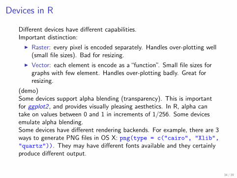
Different devices have different capabilities.Important distinction:

! Raster: every pixel is encoded separately. Handles over-plotting well(small file sizes). Bad for resizing.

! Vector: each element is encode as a“function”. Small file sizes forgraphs with few element. Handles over-plotting badly. Great forresizing.

(demo)Some devices support alpha blending (transparency). This is importantfor ggplot2 , and provides visually pleasing aesthetics. In R, alpha cantake on values between 0 and 1 in increments of 1/256. Some devicesemulate alpha blending.Some devices have different rendering backends. For example, there are 3ways to generate PNG files in OS X: png(type = c("cairo", "Xlib","quartz")). They may have different fonts available and they certainlyproduce different output.

34 / 39

Devices in R

Recently R switched to using a cairo backend (prettier graphics, morecapabilities). If on-screen plotting from the cluster is slow, try x11(type= "Xlib") instead of the default x11(type = "cairo").

35 / 39

Devices in R

Raster: png(), jpeg(), bitmap()Vector: pdf() (alpha), ps()On-screen devices: x11, quartz (OS X)Packages: rgl (OpenGL), GDD (bitmap formats), RSvgDevice, canvas(HTML canvas), RSVGTipsDevice, tikzDevice (Latex).I use quartz, quartz(type = "pdf"), and sometimes (rarely)quartz(type = "png").

36 / 39

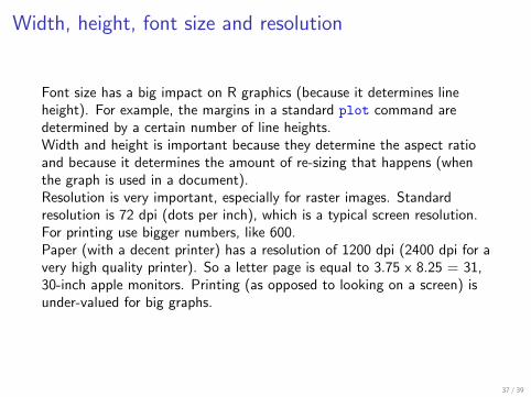
Width, height, font size and resolution

Font size has a big impact on R graphics (because it determines lineheight). For example, the margins in a standard plot command aredetermined by a certain number of line heights.Width and height is important because they determine the aspect ratioand because it determines the amount of re-sizing that happens (whenthe graph is used in a document).Resolution is very important, especially for raster images. Standardresolution is 72 dpi (dots per inch), which is a typical screen resolution.For printing use bigger numbers, like 600.Paper (with a decent printer) has a resolution of 1200 dpi (2400 dpi for avery high quality printer). So a letter page is equal to 3.75 x 8.25 = 31,30-inch apple monitors. Printing (as opposed to looking on a screen) isunder-valued for big graphs.

37 / 39

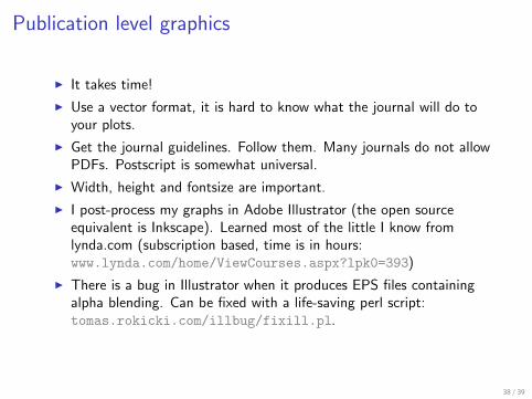
Publication level graphics

! It takes time!

! Use a vector format, it is hard to know what the journal will do toyour plots.

! Get the journal guidelines. Follow them. Many journals do not allowPDFs. Postscript is somewhat universal.

! Width, height and fontsize are important.

! I post-process my graphs in Adobe Illustrator (the open sourceequivalent is Inkscape). Learned most of the little I know fromlynda.com (subscription based, time is in hours:www.lynda.com/home/ViewCourses.aspx?lpk0=393)

! There is a bug in Illustrator when it produces EPS files containingalpha blending. Can be fixed with a life-saving perl script:tomas.rokicki.com/illbug/fixill.pl.

38 / 39

Session Info

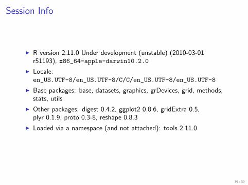
! R version 2.11.0 Under development (unstable) (2010-03-01r51193), x86_64-apple-darwin10.2.0

! Locale:en_US.UTF-8/en_US.UTF-8/C/C/en_US.UTF-8/en_US.UTF-8

! Base packages: base, datasets, graphics, grDevices, grid, methods,stats, utils

! Other packages: digest 0.4.2, ggplot2 0.8.6, gridExtra 0.5,plyr 0.1.9, proto 0.3-8, reshape 0.8.3

! Loaded via a namespace (and not attached): tools 2.11.0

39 / 39