Lehigh UniversityLehigh Preserve

Theses and Dissertations

2012

Gibbs Energy Modeling of Binary and TernaryMolten Nitrate Salt SystemsTucker ElliottLehigh University

Follow this and additional works at: http://preserve.lehigh.edu/etd

This Thesis is brought to you for free and open access by Lehigh Preserve. It has been accepted for inclusion in Theses and Dissertations by anauthorized administrator of Lehigh Preserve. For more information, please contact preserve@lehigh.edu.

Recommended CitationElliott, Tucker, "Gibbs Energy Modeling of Binary and Ternary Molten Nitrate Salt Systems" (2012). Theses and Dissertations. Paper1207.

Gibbs Energy Modeling of Binary and Ternary Molten Nitrate Salt Systems

by

Tucker R. Elliott

A Thesis

Presented to the Graduate and Research Committee

of Lehigh University

in Candidacy for the Degree of

Master of Science

in

Mechanical Engineering and Mechanics

Lehigh University

November 2011

ii

Copyright

Tucker R. Elliott

iii

This thesis is accepted and approved in partial fulfillment of the requirements for the

Master of Science.

Gibbs Energy Modeling of Binary and Ternary Molten Nitrate Salt Systems

______________________

Date Approved

_____________________________

Dr. Alparslan Oztekin

Advisor

_____________________________

Dr. Sudhakar Neti

Co-Advisor

_____________________________

Dr. D. Gary Harlow

Department Chairperson

iv

ACKNOWLEDGEMENTS

I would like to thank Dr. Alparslan Oztekin and Dr. Sudhakar Neti for their continuous

support throughout this research project and their guidance regarding this thesis. They have been

an invaluable source of information. Additionally, I would like to thank Dr. Satish Mohapatra

and Dynalene Inc. for sponsoring the project, as well providing suggestions and experimental

data to improve my work.

Finally, I would like to thank Walter and Patti Ann, my father and mother, who enabled

me to be in the position that I am today.

v

TABLE OF CONTENTS

Page

Acknowledgements .................................................................................................................... iv

List of Figures ............................................................................................................................. vi

List of Tables ............................................................................................................................. vii

Abstract .........................................................................................................................................1

Chapter 1. Introduction ................................................................................................................ 2

Chapter 2. Background Literature ................................................................................................ 5

Chapter 3. Experimental Methods ................................................................................................7

Chapter 4. Mathematical Model and Numerical Method ............................................................ 9

Chapter 5. Results and Discussion ............................................................................................. 29

Chapter 6. Conclusions .............................................................................................................. 45

Chapter 7. Further Research ...................................................................................................... 47

List of References ...................................................................................................................... 48

Vita ............................................................................................................................................. 50

vi

List of Figures

Page

Figure 1. Effect of solid enthalpy of mixing coefficient values on phase diagram shape ..........15

Figure 2. NaNO3-KNO3 simulated phase diagram compared against Coscia experimental data ...

.....................................................................................................................................................30

Figure 3. LiNO3-NaNO3 simulated phase diagram compared against Coscia experimental data ..

.....................................................................................................................................................31

Figure 4. LiNO3-KNO3 simulated phase diagram compared against Coscia experimental data ....

.....................................................................................................................................................32

Figure 5. NaNO3-KNO3 simulated phase diagram compared against Zhang experimental data ...

.....................................................................................................................................................33

Figure 6. LiNO3-NaNO3 simulated phase diagram compared against Campbell and Vallet

experimental data ....................................................................................................................... 34

Figure 7. LiNO3-KNO3 simulated phase diagram compared against Zhang and Vallet

experimental data ........................................................................................................................35

Figure 8. LiNO3-NaNO3-KNO3 system predicted phase diagram - lower values ......................36

Figure 9. LiNO3-NaNO3-KNO3 system predicted phase diagram - higher values .....................37

Figure 10. LiNO3-NaNO3-KNO3 system predicted solidus curves ............................................38

Figure 11a. Ternary phase diagram surface plot .........................................................................39

Figure 11b. Ternary phase diagram surface plot ........................................................................40

Figure 11c. Ternary phase diagram surface plot .........................................................................40

Figure 12. Top view of ternary phase diagram ...........................................................................41

Figure 13. LiNO3-NaNO3-KNO3 simulated phase diagram compared against experimental data -

lower values ................................................................................................................................42

Figure 14. LiNO3-NaNO3-KNO3 simulated phase diagram compared against experimental data -

higher values ...............................................................................................................................43

vii

List of Tables

Page

Table 1. Salt property values ..................................................................................................... 28

Table 2. Enthalpy of mixing empirical coefficient values ......................................................... 29

1

Abstract

Molten nitrate salts have the potential to become efficient heat transfer fluids in many

applications, including concentrated solar power plants and in energy storage systems. Their low

melting temperatures and high energy densities contribute to this. Thus, an understanding of the

phase diagrams of these salts is important, specifically, knowledge of the melting and freezing

temperatures of these mixtures at various concentrations. Many previous works have investigated

modeling these phase diagrams, particularly binary mixtures of nitrate salts. Ternary simulations

for molten salts exist but results have been limited. Using existing enthalpy of mixing data for

binary mixtures, an accurate ternary phase diagram has been constructed. The binary systems

NaNO3- KNO3, LiNO3- NaNO3, and LiNO3- KNO3 and the ternary system LiNO3-NaNO3-

KNO3 have been modeled using a Gibbs energy minimization method. The predictions from this

present model agree well with the results of experiments by our group and the data collected by

previous researchers. The ternary predictions constructed using only binary interactions, agree

reasonably well with the experimental data collected by our group. It is determined that the

ternary mixture has a eutectic temperature of 107° Celsius at a composition of 43-47-10 mole

percent LiNO3-KNO3-NaNO3 respectively, and will be a viable heat transfer fluid. The

thermodynamic model used here can be applied to any ternary system as well as any higher-

order component system.

2

Chapter 1. Introduction

As the world looks to decrease fossil fuel usage, the need for a clean renewable energy

source has become more apparent. Solar thermal energy is one such alternative energy choice. In

2007, of all the energy utilized in the United States, only 7% came from renewable sources. And

of that, only 1% was from solar sources [1]. The market for solar thermal energy is therefore

young. For solar thermal energy to become a more viable technology, a heat transfer fluid with a

high energy density and low melting point is desired. The molten nitrate salts presented here

have such qualities. Binary and ternary systems of nitrate salts have lower melting temperatures

than single component nitrate salts and as a result need less inputted energy to remain molten.

During the night or a cloudy day, when no sunlight is available, less energy from the grid is

needed to heat the fluid. This can keep costs down for a solar power plant, for example. In

addition, using the eutectic composition of a binary or ternary salt, means the lowest melting

point of that salt is utilized. Therefore at the eutectic temperature, the smallest amount of

inputted energy is needed to keep the salt in the liquid state. Nitrate salts were chosen over other

salts for their high energy density, stability at high temperatures, and their relatively low melting

points [2].

Molten salts can be used in different solar thermal applications as heat transfer fluids.

One example is in a parabolic trough system. The molten salt flows through a piping scheme

which is placed at the focal point of a parabolic mirror. The sun's rays are deflected from the

mirror and are focused on the tube so that the flowing salt will absorb the thermal energy.

Another application of molten salt as a working fluid is in a power tower plant. Heliostats are

placed around a tower with a receiver. The mirrors are all aimed to the receiver where the molten

salt is flowing past in a pipe. Again the molten salt will absorb the thermal energy from the sun.

3

In both scenarios, the hot molten salt is used to heat water into steam in a Brayton cycle. The

Brayton cycle will produce electricity which can be inputted into the electric grid.

Knowledge of the chemistry of the molten salts in question is necessary in both an

efficiency sense and a business sense. One of the main goals is to produce a salt with a low

melting temperature. Operating a concentrated solar power plant using a working fluid with a

low melting temperature will be more efficient than using a similar salt with a higher melting

temperature because the plant will use less energy.

In nitrate salt mixtures, eutectic points exist. A eutectic point is where, at a specific

chemical composition, the system solidifies at a lower temperature than at any other composition

[3]. At the eutectic point, the liquid mixture of the two components is in equilibrium with the

crystals of each component. If the temperature is lowered past the eutectic temperature, each

component will begin to crystallize out of the mixture [4]. Using a salt with a composition at or

near its eutectic composition will have a lower melting temperature than, for instance, using a

pure salt. Subsequently, information about the eutectic compositions of different salt systems is

desired.

Experimental data exist for some salt systems, mainly binary systems, but not all. Data on

ternary systems is also present but not fully known. Differential scanning calorimetry

experiments can be conducted to find melting temperatures of salts at different compositions and

eventually with enough experimental data, phase diagrams can be constructed. This process can

be tedious and costly. Care must be taken to buy and use salts with little impurities, and also to

accurately mix salts with the desired concentrations. Testing many different compositions of

different salt mixtures will be time consuming. If accurate predictions of salt phase diagrams can

4

be made instead, the time and money consumed to experimentally produce these phase diagrams

can be saved.

This present research puts forward modeling phase diagrams using a Gibbs function

minimization technique. The Gibbs function is defined as the difference between the enthalpy

and product of the temperature and entropy, as shown below.

(1)

The Gibbs function, also known as, Gibbs free energy is used to determine whether or not

a system is in equilibrium, and the composition at which it will occur. This is used as the basis

for the modeling illustrated below.

The structure of this thesis will be as follows. Chapter two will present background

literature that was used as a starting point for this work. Chapter three will delve into the

methods employed to generate the experimental data against which our models were compared.

Chapter four will discuss the mathematical model used to predict the phase diagrams of the

nitrate salts studied, and the numerical method that executed this. Chapter five will examine the

results of the predictions and will compare these to empirical data. The conclusions of this work

will be presented in chapter six, and in chapter seven suggestions for future work will be

provided.

5

Chapter 2. Background Literature

The assertion that molten nitrate salts would be very useful in energy storage systems as

well as in solar thermal energy applications as a working fluid is not relatively novel, but has

been known for some time [5]. Despite this, there was an admitted lack of information on the

properties of these salts [6]. With advancements in differential scanning calorimetry technology

and other methods, more experimental data has surfaced [7]. In addition to property data, many

attempts to calculate phase diagrams have been purported. This is seen in CALPHAD and other

methods [8].

Some of the previous works that have studied the phase diagrams of selected nitrate salts

are mentioned below. O.J. Kleppa and L.S. Hersh [6,9] studied the heats of mixing in liquid

alkali nitrate salt systems in 1960. More specifically, they studied binary salt systems with nitrate

being the common anion. Using a high-temperature reaction calorimeter, measurements of the

heats of mixing were taken. Kleppa's empirical values for the heat of mixing data were used a

basis for the phase diagram modeling here.

In addition, C.M. Kramer and C.J. Wilson [5] examined the phase diagram of the sodium

nitrate-potassium nitrate binary system. Their theoretical derivation, that the solid and liquid

solutions of a system are in equilibrium when the free energy is set equal to zero, was used as a

starting point for our mathematical model. This was used to study other binary nitrate systems

and the more complicated ternary system.

More recently, Xuejan Zhang et al. [10,11] investigated the phase diagrams of the

lithium-potassium nitrate and sodium-potassium nitrate systems in 2001 and 2003, respectively.

Again, their thermodynamic relationships served as a basis for the modeling here and was in

agreement with the relationships observed in previous works.

6

The experimental data produced by Zhang [10,11], A. N. Campbell et al. [12], and C.

Vallet [13], was used as a comparison with the phase diagrams predicted here and also with the

experimental data that was produced by our group, which will be discussed in the next section.

Their data served as another check to the accuracy of the collection methods of our group and to

the phase diagram simulations that were produced.

Data for the lithium-sodium-potassium nitrate ternary salt was limited, and modeling

attempts were hard to find. A journal piece by A. G. Bergman and K. Nogoev [14] presents

experimental data on the ternary system. This data is once more used a reference for the ternary

system modeling and data collection shown here.

The literature above provided a starting ground for the results illustrated here and this

present research expands upon these previous works.

7

Chapter 3. Experimental Methods

Experiments were conducted to determine phase diagrams of the salt mixtures

investigated in this present work. Research engineers from Dynalene Inc., an industrial heat

transfer fluid manufacturer, teamed up with students and faculty from Lehigh University to study

nitrate salts. The research included determining the properties of these salts and the modeling of

their phase diagrams. The results of the present calculations have been compared with the

experiments conducted at Dynalene [15,16]. A discussion of these experiments is provided here.

Using the equipment and resources at Dynalene Inc., the experiments were made

possible. Differential scanning calorimetry (DSC) was used to determine the phase diagrams of

the salt mixtures. DSC is a measuring technique used to determine temperatures as well as heat

flows during phase changes, such as melting or crystallization [7]. The differential scanning

calorimeter used here was the TA DSC Q200. Because of the temperature limitations of the

machine, isothermal runs were only performed to 400°C. Phase transitions were calibrated using

high purity indium.

The salts used were American Chemical Society (ACS) grade lithium, sodium, and

potassium nitrate. These salts were dried in a furnace at 150°C for 24 hours and stored over a

desiccant to ensure purity. The dried salts were measure out using a Mettler-Toledo XS-205

analytical balance which carried out masses to ±0.001 grams; this guaranteed the accuracy of the

ratio of the salts being measured.

After measurement, the binary mixtures were placed in a furnace to fuse at 350°C for at

least 24 hours, to obtain sufficient homogenization. Ternary mixtures were kept there for 48

hours to ensure uniformity due to the addition of the third component. The experimenter notes

that exposing the salts to these temperatures for that period of time did not initiate thermal

8

degradation based on evidence from previous experiments and reports from literature. Each salt

mixture was tested by the DSC three times, with more runs performed for mixtures close to the

suspected eutectic composition.

The framework of each salt sample was established by using a heating rate of 10°C/min

to provide a general idea of where to look for the solidus and liquidus points on the DSC plot.

Melting runs were carried out to 320°C and then cooled to the original holding temperature at a

rate of 5°C/min. Upon heating, the solidus for each plot is defined as the first deviation from the

baseline and the liquidus is defined as the largest signal of the last thermal event prior to its

return to the baseline. Upon cooling, the liquidus is defined as the first deviation from the

baseline and the solidus is the deviation from the last thermal event prior to returning to the

baseline.

9

Chapter 4. Mathematical Model

4.1 Binary Formulation

Modeling a binary system, begins with setting the Gibbs free energy of the system equal

to zero [5]. In a system with two components, A and B, this is done for each component. The

free energy consists of three terms: first, the fusion term, second, the free energy of mixing of

the liquid solution, and finally the free energy of mixing of the solid solution. Because the free

energy is set to zero, both the liquid and solid solutions of each component are in thermodynamic

equilibrium. For example, the free energy of component A is expressed as

- -

- -

(2)

where, as described above, it is seen split into three terms [5].

Expanding the components of the first term leads to

- -

(3)

and

- -

(4)

where and

are the enthalpy and entropy of fusion of component A, respectively, at its

melting point. To account for the temperature difference between the salt's current temperature

and its melting temperature, a correction term is needed. The correction terms use the difference

in specific heat between the liquid ( ) and solid ( ) phases. The correction terms are

integrated over the temperature range, starting from the component's melting temperature to the

current temperature at which the equation is being solved. Integration of the enthalpy equation

leads to

(5)

10

where is used to denote the difference between and . The melting temperature of the

component is represented as and is the current temperature of the system. Next, the

equation below is used to relate the entropy of fusion to the enthalpy of fusion of component A.

(6)

Integration of the entropy equation and application of the above substitution for leads to

(7)

Now that the terms and have been expanded, these expressions can be plugged into the

first term of the Gibbs free energy equation, shown below.

-

(8)

Rearranging this equation and it becomes,

-

(9)

The Gibbs-Duhem equation must be utilized to determine in both the liquid and

solid phases [5]. The Gibbs-Duhem equation, for component A, is defined as follows

-

(10)

where, the enthalpy of mixing, , in its most general manner, is expressed as a polynomial

of the form

(11)

Here and are the mole fractions of each component with as the component with the

smaller cation. The letters a, b, and c represent empirical coefficients. Determination of these

coefficients is discussed later. The second term in the Gibbs-Duhem equation, shown above, is

the product of - and the total derivative of the enthalpy of mixing, , taken with

11

respect to . Taking the derivative correctly (with respect to ) requires that - is

substituted in for each . This is done because is related to and this effect must be taken

into account. Applying this substitution and then taking the derivative results in

(12)

Plugging this derivative into the Gibbs-Duhem equation, and after cancelling of like terms, the

partial molar enthalpy of mixing for component A becomes,

(13)

This same procedure is applied to each phase, both the liquid and the solid. To determine the

partial molar enthalpy of mixing for component B, the Gibbs-Duhem equation is again used, this

time of the form

-

(14)

Expanding this term is accomplished in the same manner as it was for component A.

The partial molar entropy of mixing in the liquid and solid phases for component A

becomes

- (15)

where is either the mole fraction of component A on the liquidus curve for the liquid phase or

the mole fraction of A on the solidus curve for the solid phase. R represents the universal gas

constant. Similarly, for component B, the expression becomes,

- (16)

Again, is the mole fraction of component B either on the liquidus or solidus curve depending

on the phase. This is the expression because the mixture is assumed to be a regular solution [5].

12

Combining the above terms produces the Gibbs free energy for a component. For

component A, this becomes

(17)

where empirical coefficients with the l and s subscripts are from the liquid and solid enthalpies

of mixing respectively. A similar equation can be developed for component B.

Currently, there are only two equations for five unknowns,

and . Two

more equations come from the relation between the concentrations of the components in each

phase. They are related as follows

(18)

(19)

where the l and s represent the liquid and solid phase, respectively. There is still one more

unknown than there are equations. In order to solve the four equations, one of the unknowns

must be given. When one of these is known, the four equations are solved simultaneously at each

composition (or temperature) to produce the phase diagrams.

4.2 Coefficients

Empirical coefficients are needed to properly represent the partial molar enthalpies of

mixing for both the solid and liquid phases. Kleppa [6] was able to experimentally derive the

expressions and coefficients for the enthalpy of mixing for various binary mixtures. He

conducted mixing experiments of different alkali nitrate salts and using the least squares method,

he was able to determine values for the empirical coefficients of the enthalpy of mixing for the

liquid phase. These values provided the basis for coefficients used in the present work.

13

Specifically, his data for the NaNO3- KNO3, LiNO3-NaNO3, and LiNO3- KNO3 binary systems

was used.

Kleppa though, did not provide values for the coefficients of the enthalpy of mixing for

the solid phase. Kramer [5], in his 1980's paper on the NaNO3- KNO3 system, modeled the

binary salt and did give an expression for the enthalpy of mixing for the solid phase. This was

used as the expression for the solid phase enthalpy of mixing here, but also as a base value for

the other two binary systems.

In order to more accurately match the phase diagram simulations to the experimental data

that was obtained, slight changes to some of Kleppa's liquid coefficients were made. Changes in

the values of the coefficients had some predictable effects on the phase diagram's shape. A

change in the magnitude of the 'a' coefficient caused the eutectic point to be shifted either up or

down in temperature. Increasing it, decreased the eutectic temperature, while decreasing the

magnitude increased the eutectic temperature. The magnitude of the 'b' coefficient affects the

symmetry of the liquidus curve around the eutectic point. So, increasing (decreasing) this

magnitude shifts the eutectic to the left (right) on a phase diagram, resulting in a different

concentration being the eutectic concentration. And the addition of the 'c' coefficient is needed

when there is a large temperature difference between the pure salt's melting temperature and the

eutectic temperature. It ensures that the modeling will be more accurate. The 'c' coefficient is

present in the LiNO3- KNO3 enthalpy of mixing expression, because for this phase diagram a

change in the composition has a larger effect on the corresponding temperature compared to the

other two binary systems.

It should also be noted that results described above were the main effect observed by the

changes in the coefficients, but by no means were they the only effects identified. While a

14

change in the 'a' coefficient did predominantly effect the temperature of the eutectic, it did to

some extent also change the composition. Likewise, a modification of the 'b' coefficient did

slightly effect the eutectic temperature in addition to primarily changing the eutectic

composition.

The solid coefficients of the enthalpy of mixing were chosen accordingly to, as expected,

agree with the experimental data. Some observations were made when choosing the solid

coefficients as well. Drastic changes in the value of the solid coefficients did have some effect on

the shape of liquidus curves and the location of the eutectic, while changes in the value of the

liquid coefficients had only marginal effects on the solidus curves. In addition, changes in the 'a'

coefficient only, or the 'b' coefficient only, had a similar effect on the solidus curves. Hence,

changes in the solid coefficients had a combined effect; the larger the magnitude of these

coefficients and the solidus curves were shifted outward towards the pure component's

composition, and had much steeper slopes. Conversely, smaller magnitudes resulted in curves

that bent in toward the eutectic point with shallower slopes. This effect can be seen in the phase

diagram below.

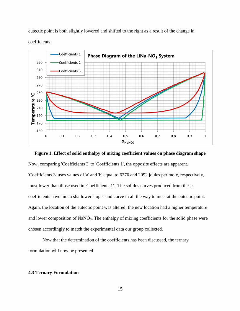
An example of the LiNO3-NaNO3 phase diagram is shown. Three different sets of solid

enthalpy of mixing coefficients were used while the liquid empirical coefficients were kept

constant. The first set, graphed as 'Coefficients 1' has intermediate values of the 'a' and 'b'

coefficients, being 9204.8 and 3347.2 joules per mole respectively. The second set, graphed as

'Coefficients 2', was produced from 'a' equal to 12,552 joules per mole and 'b' equal to 6276

joules per mole. Compared to 'Coefficients 1', 'Coefficients 2' contains solidus curves which are

very vertical and do not bend in towards the eutectic point at all. In addition, the resulting

15

eutectic point is both slightly lowered and shifted to the right as a result of the change in

coefficients.

Figure 1. Effect of solid enthalpy of mixing coefficient values on phase diagram shape

Now, comparing 'Coefficients 3' to 'Coefficients 1', the opposite effects are apparent.

'Coefficients 3' uses values of 'a' and 'b' equal to 6276 and 2092 joules per mole, respectively,

must lower than those used in 'Coefficients 1' . The solidus curves produced from these

coefficients have much shallower slopes and curve in all the way to meet at the eutectic point.

Again, the location of the eutectic point was altered; the new location had a higher temperature

and lower composition of NaNO3. The enthalpy of mixing coefficients for the solid phase were

chosen accordingly to match the experimental data our group collected.

Now that the determination of the coefficients has been discussed, the ternary

formulation will now be presented.

4.3 Ternary Formulation

150

170

190

210

230

250

270

290

310

330

0 0.1 0.2 0.3 0.4 0.5 0.6 0.7 0.8 0.9 1

Tem

pera

ture

°C

xNaNO3

Phase Diagram of the LiNa-NO3 System Coefficients 1

Coefficients 2

Coefficients 3

16

In a ternary system of nitrate salts, the Gibbs free energy of each component is set equal

to zero. Again, as in a binary system, the solid and liquid phases of each component are in

thermodynamic equilibrium, and each component is in equilibrium with the other. At each

composition of the salt, there are five equations that need to be satisfied. First, the free energy of

all three components must be fulfilled, and then the relation between the component's

compositions in the both liquid and solid phases provide the last two equations. Consequently,

there are seven unknowns and only five equations. Therefore, the compositions of two of the

components must be known. Solving these five equations simultaneously provides solutions for

the liquid and solid compositions for each component and the temperature at these compositions.

As in a binary system, the free energy of a component A, for example, becomes,

- -

- -

(20)

and the same expressions exist for the other two components. Expansion of each of these terms is

completed using the same approach to that of the binary system. Determining the partial enthalpy

of mixing for each component is a bit more complex. The enthalpy of mixing for the ternary

system is expressed as the addition of the three binary mixing interactions. The ternary

interaction of the three components is assumed to be negligible compared to the binary

interactions and is therefore omitted. Further research can be conducted into the ternary

interaction to validate this claim. Expansion of the enthalpy of mixing of the liquid phase for the

ternary system is shown below. The form used is

(21)

where is equivalent to as seen in the binary formulation. This is expanded as

(22)

17

where and represent the liquid concentrations of NaNO3, KNO3, and LiNO3

respectively. The coefficients here are those from the three binary systems. The presence of the c

coefficient in the LiNO3-KNO3 expressions and not the others is due to the large temperature

difference between the eutectic and the pure component's melting temperatures. Again, the

Gibbs-Duhem equation must be applied to determine the partial molar enthalpy of mixing for

each component. For component A, the form of the equation used is shown below

(23)

For this equation to be valid, the ratio of the two other liquid concentrations must be kept

constant. This ratio will be known as C, as seen below

(24)

This must be done to ensure that when taking the partial derivative, that the effects of the other

components are kept constant. Here

is the partial derivative of

taken with respect to

component A. The differentiation is illustrated here,

(25)

Combining like terms,

(26)

Next, the terms

and

must be evaluated and expressed in terms of the concentrations. To

do this, the equation below is utilized.

18

(27)

The substitution

is used for and after rearranging, the equation becomes,

(28)

Dividing both sides by the value

and it produces

(29)

After differentiation with respect to component A, and substituting back in for

(30)

And finally, rearranging the right side of the equation and substituting, for the

equation becomes

(31)

A similar procedure is followed to determine

. Again, starting with the equation below, but

now utilizing the substitution .

(32)

Substituting and rearranging,

(33)

Dividing both sides by the value and it produces

(34)

After differentiation with respect to component B, and substituting back in for

(35)

19

And again, rearranging the right side of the equation and substituting, for the

equation becomes

(36)

These two results are now substituted into the enthalpy of mixing equation as seen below.

(37)

Simplifying,

(38)

Now substituting in for

and again simplifying,

(39)

And finally, after crossing out like terms the final form the partial enthalpy of mixing for

component A is produced,

(40)

This same method is used for components B and C. For component B, the form of the

Gibbs-Duhem equation that is used is

(41)

where now, the ratio between the liquid concentrations of components A and C is held constant

as seen below,

20

(42)

Here

is the partial derivative of

taken with respect to component B. The differentiation

is illustrated here,

(43)

After rearranging like terms together,

(44)

Again, the terms

and

must be evaluated and expressed in terms of the concentrations.

This process is the same as it was for component A, as demonstrated above. The final forms for

each term are

(45)

and

(46)

Plugging these into the equation above, and after simplifying,

(47)

And finally, after plugging in

and simplifying, the result for the partial molar enthalpy of

mixing for component B becomes,

21

(48)

On to component C, where the form of the Gibbs-Duhem equation is now

(49)

where the constant C is now equal to the ratio between the liquid concentrations of components

A and B,

(50)

After differentiation,

(51)

The two terms

and

must again be expressed in terms of the component's concentrations.

Again, this process is the same as it was for component A, and is demonstrated above. The final

forms for each term become,

(52)

and

(53)

Now, using these two terms and after some simplification,

(54)

Plugging in for

and after more simplification, the final form for the partial molar enthalpy

of mixing for component C is obtained,

22

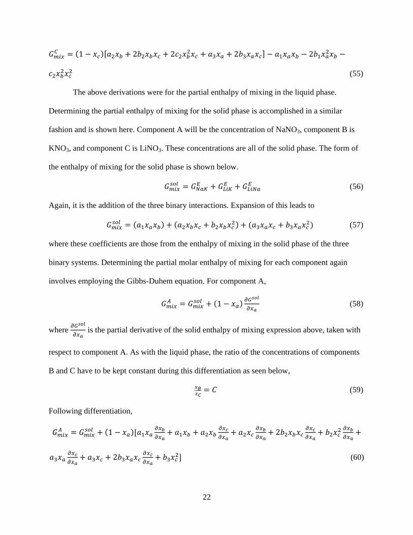
(55)

The above derivations were for the partial enthalpy of mixing in the liquid phase.

Determining the partial enthalpy of mixing for the solid phase is accomplished in a similar

fashion and is shown here. Component A will be the concentration of NaNO3, component B is

KNO3, and component C is LiNO3. These concentrations are all of the solid phase. The form of

the enthalpy of mixing for the solid phase is shown below.

(56)

Again, it is the addition of the three binary interactions. Expansion of this leads to

(57)

where these coefficients are those from the enthalpy of mixing in the solid phase of the three

binary systems. Determining the partial molar enthalpy of mixing for each component again

involves employing the Gibbs-Duhem equation. For component A,

(58)

where

is the partial derivative of the solid enthalpy of mixing expression above, taken with

respect to component A. As with the liquid phase, the ratio of the concentrations of components

B and C have to be kept constant during this differentiation as seen below,

(59)

Following differentiation,

(60)

23

The terms

and

again need to be expanded, and the expansions are exactly the same as

they are for component A in the liquid solution, are reproduced below.

(61)

(62)

Rearranging and substituting in the above equations,

(63)

Simplifying and substituting in for ,

(64)

And finally canceling out like terms, the final form for component A is,

Again for component B, the Gibbs-Duhem equation becomes,

(65)

where the ratio between the concentrations of components A and C is kept constant.

Differentiating and the expression becomes,

(66)

The substitutions for

and

again are the same as that for component B in the liquid phase,

seen below

24

(67)

(68)

Applying this substitution and simplifying,

(69)

Finally, after substitution for and canceling out like terms the expression becomes,

(70)

And lastly, for component C, the Gibbs-Duhem equation is of the form,

(71)

with the ratio of component A to component B being kept constant. Following differentiation,

(72)

Again the expressions (which are the same as those for component C in the liquid solution)

below are used,

(73)

(74)

After substitution and rearrangement,

(75)

And finally, after the substitution for and simplifying, the final form for the enthalpy of

mixing of the solid solution for component C becomes,

25

(76)

Now that each of the terms for the Gibbs free energy for each component have been expanded,

they are put together. For component A,

(77)

For component B,

(78)

And for component C,

(79)

The a, b, and c coefficients within the first set of parentheses for each component are the

liquid enthalpy of mixing empirical coefficients, while the coefficients within the last set of

parentheses are the solid enthalpy of mixing empirical coefficients.

The final two equations which relate the concentrations of each component are

(80)

(81)

26

where the superscripts l and s stand for the liquid and solid phases, respectively. Solving these

equations is discussed in the section below.

4.4 Numerical Method

A computer program was written in the numerical computing software MATLAB, to

simultaneously solve the four binary simulation equations at various concentrations of each

component. Due to the fact that there are five unknowns for the four equations, one of these

unknowns must be inputted into the program. In order to solve these equations, certain properties

of the pure salts must also be known. These include the molar mass, the melting temperature, the

latent heat of fusion, and the specific heat in the liquid and solid phases. The values used are

reproduced in table 1 below. These values were all assumed to be constant within the

temperature range of the phase diagram. The inputted unknown is the liquid concentration of one

of the components.

For instance, in the NaNO3-KNO3 system, the liquid concentration of KNO3 is inputted

into the program ranging from 1 to 99 percent mole KNO3 (the percents 0 and 100 cannot

explicitly be inputted, or the program will fail, but very small or very large mole percentages can

be entered to estimate those values). The program will solve for the remaining four unknowns at

each inputted composition, namely, the other liquidus concentration, the two solidus

concentrations, and the temperature.

Solving these equations in MATLAB is accomplished using the built-in function solver

called fsolve. It is used to solve systems of non-linear equations. The solver uses a trust-region

dogleg algorithm to accomplish this. Information on this algorithm is provided by MATLAB.

[19]. The equations are rewritten in the form

27

(82)

and the solver will find the roots of the equations. Initial guesses need to be provided to the

solver at each concentration, so the desired roots can be found more easily and accurately. The

first guess is inputted manually because, for example, at 1 mole percentage KNO3 in the NaNO3-

KNO3 system, the solidification temperature and the relative amounts of the two solidus

concentrations are all known (due to this concentration being so close to pure NaNO3). After the

solver outputs the roots to the equations at this concentration, it now uses these solutions as the

initial guesses for the next concentration. And this is done throughout the whole range of

inputted concentrations to ensure that the solver can find the roots quickly and efficiently.

To produce a full phase diagram the KNO3 concentration is incremented by 1 mole

percentage, starting from 1 and ending at 99 mole percent, with the calculations being performed

at each increment. This data is then plotted to produce the simulated phase diagram.

As will be presented below, solutions to each of the three binary phase diagrams were not

always continuous. Only in the NaNO3-KNO3 system were the solidus and liquidus lines

continuous. For this system, the inputted concentration can be started at either end of the phase

diagram and be continued all the way through to opposite side, and a solution will be found at

each increment without the solver function failing to find a solution. Both the solidus and

liquidus line both connect at the eutectic point, with a continuous slope on each side of the point.

This is not the case with either the LiNO3-NaNO3 or LiNO3-KNO3 systems. For these

systems, each side of the phase diagram had to be solved separately. If the inputted concentration

was ranged from 1 to 99 percent in a single run of the program, the solver would fail near

concentrations past the eutectic point because it won't be able to find solution. If solutions were

found, they would either include concentrations above unity or imaginary numbers, both of

28

which do not have any physical meaning. These roots were therefore discarded. So to solve for

the phase diagrams of these system, each side of the diagram had to be solved independently.

One script was written which inputted concentrations starting at the left side of the diagram, and

another script starting at the right side of the diagram. The eutectic point of these two systems

was determined to be the point of intersection between the two liquidus curves that were solved

for separately. Also, the solidus curves in these systems showed a discontinuity in their slopes.

They start out as curves but when they reach the eutectic temperature they become flat for a large

range of compositions. But according to experimental data here and by others this is relatively

common.

The salt property constants that were used for the modeling are shown in the table below.

Salt

Molar Mass

(g/mol)

Melting Temperature

(Kelvin)

Latent Heat

(J/g)

Cp(l) - Cp(s)

(J/gK)

NaNO3 84.9947 577.5 173 -0.11

KNO3 101.103 607.4 96.6 -0.03

LiNO3 68.946 525.9 363 0.25

Table 1. Salt property values

The molar mass values used are well documented. The melting temperatures as well as the latent

heats (enthalpies of fusion) of the components were taken from a reference by Y. Takahashi et al.

[17]. The specific heat differences between the liquid and solid states of the salts were those

measured by M. J. Maeso and J. Largo [18].

29

Chapter 5. Results and Discussion

5.1 Binary System

The phase diagram predictions for all three binary systems were produced and compared

against experimental data. The first comparisons are against the data collected at Dynalene Inc.,

by Kevin Coscia. The values of the empirical constants used for each system are shown in the

table below.

Salt System

Δ mix, liquid Δ mix, solid

a b c a b c

NaNO3:KNO3 -1707 -284.5 0 6276 0 0

LiNO3:NaNO3 -1941.4 -2928.8 0 9204.8 3347.2 0

LiNO3:KNO3 -9183.9 -364 -1937.2 10460 4184 0

Table 2. Enthalpy of mixing empirical coefficient values

There is no b coefficient for the NaNO3-KNO3 solid enthalpy of mixing expression, due

to the symmetry present in this system that is not seen in the other two mixtures. Additionally,

the only binary system with a c coefficient is the LiNO3-KNO3 mixture, because it has the largest

temperature difference between the eutectic temperature and pure component melting

temperature. This extra coefficient enables a better fit between the predictions and experimental

data shown here.

The sodium-potassium nitrate binary system is displayed in the figure below.

30

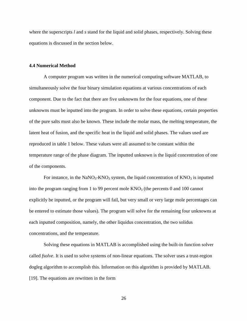
Figure 2. NaNO3-KNO3 simulated phase diagram compared against Coscia experimental

data

Due to the continuous nature of this phase diagram, it displayed the closest fit to the

experimental data. The data indicates a eutectic point is present at 50 mol% KNO3 and 50 mol%

NaNO3 at a temperature of 222°C. The solid solubility of the system is also included; here it is

seen as the group of data points at the eutectic temperature, ranging in composition from 20

mol% to 80 mol% KNO3.

Using the thermodynamic model, the eutectic point was calculated to be at a temperature

of 220.4°C with compositions of 52.1 mol% KNO3 and 47.9 mol% NaNO3. There is a minor

discrepancy in the location of the eutectic point with the model predicting slightly more KNO3

present and also at a faintly higher temperature. The predicted eutectic composition is within 5

percent error, while the predicted temperature is within 1 percent error.

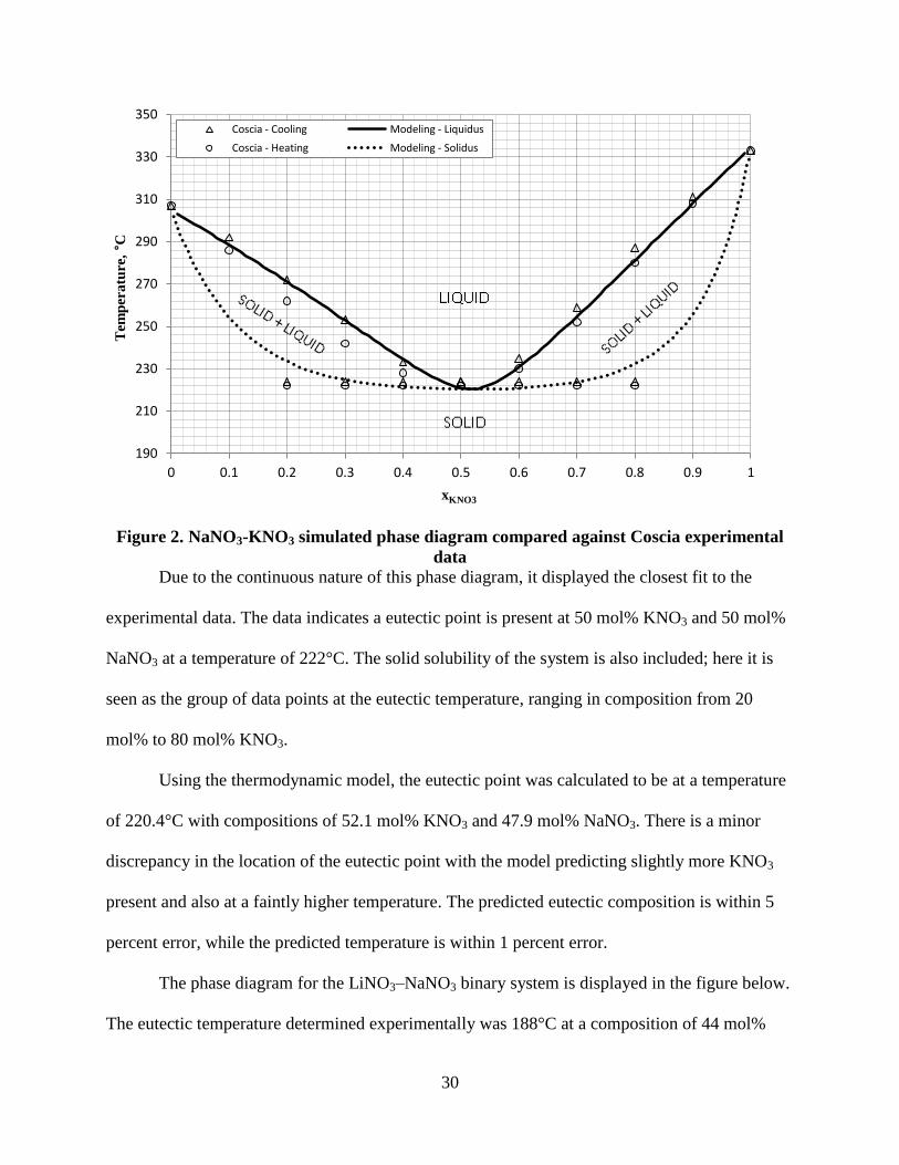
The phase diagram for the LiNO3–NaNO3 binary system is displayed in the figure below.

The eutectic temperature determined experimentally was 188°C at a composition of 44 mol%

190

210

230

250

270

290

310

330

350

0 0.1 0.2 0.3 0.4 0.5 0.6 0.7 0.8 0.9 1

Tem

per

atu

re, °C

xKNO3

Coscia - Cooling Modeling - Liquidus

Coscia - Heating Modeling - Solidus

31

NaNO3 and 56 mol% LiNO3. Again the solidus line is seen as the horizontal points ranging from

10 to 90 mol% NaNO3, at the eutectic temperature.

Figure 3. LiNO3-NaNO3 simulated phase diagram compared against Coscia experimental

data

The simulated eutectic point was determined at a composition of 46 mol% NaNO3 at 183°C.

This eutectic composition had a larger value of NaNO3 and the eutectic composition was at a

lower temperature. The modeled eutectic composition was within 5 percent error of the

experimental data and the modeled eutectic temperature are within 3 percent error of the

experimental data.

The experimental data for the LiNO3–KNO3 binary system is displayed in the figure

below. For this system the eutectic composition was experimentally determined to be 42.5 mol%

LiNO3 and 57.5 mol% KNO3 at a temperature of 115°C. Again, the solidus line is constant at the

eutectic temperature.

150

170

190

210

230

250

270

290

310

330

0 0.1 0.2 0.3 0.4 0.5 0.6 0.7 0.8 0.9 1

Tem

per

atu

re, °C

xNaNO3

Coscia - Cooling Modeling - Liquidus

Coscia - Heating Modeling - Solidus

32

Figure 4. LiNO3-KNO3 simulated phase diagram compared against Coscia experimental

data

The simulations produce a eutectic composition of 44 mol% LiNO3 and 56 mol% KNO3 at a

temperature 122°C. Here, the predicted eutectic composition contains a lower amount of KNO3,

while the predicted eutectic temperature was greater. The calculated eutectic composition is

within 3 percent error and the calculated temperature is within 5 percent error.

Each of these predicted phase diagrams showed great agreement with the experimental

data that was collected. At compositions closer to the pure components, the agreement was

excellent and a bit better than compared to compositions closer to the eutectic point, although the

agreement near the eutectic point is still very good. The predicted phase diagrams will now be

compared to experimental data recorded by others.

5.2 Binary Comparison with other Experimenters

The NaNO3-KNO3 system produced by Zhang et al. [11] is compared to our

thermodynamic model's predictions. The results are shown below.

50

100

150

200

250

300

350

0 0.1 0.2 0.3 0.4 0.5 0.6 0.7 0.8 0.9 1

Tem

per

atu

re, °C

xKNO3

Coscia - Cooling Modeling - Liquidus

Coscia - Heating Modeling - Solidus

33

Figure 5. NaNO3-KNO3 simulated phase diagram compared against Zhang experimental

data

The predicted eutectic composition and temperature are in very good agreement with Zhang.

Some discrepancies do exist in both the liquidus and solidus curves. Zhang's data indicates that

the liquidus values follows a near linear trend in contrast to the non-linear trend that our model

produces. In addition he observed the solidus line as staying constant closer to each end of the

phase diagram, whereas in our model the solidus follows a curved path.

Our predicted LiNO3-NaNO3 model is compared against the experimental data of both

Campbell et al. [12] and Vallet [13].

190

210

230

250

270

290

310

330

350

0 0.1 0.2 0.3 0.4 0.5 0.6 0.7 0.8 0.9 1

Tem

pera

ture

, °C

xKNO3

Phase Diagram of the NaK-NO3 System Zhang - Liquidus

Zhang - Solidus

Modeling - Liquidus

Modeling - Solidus

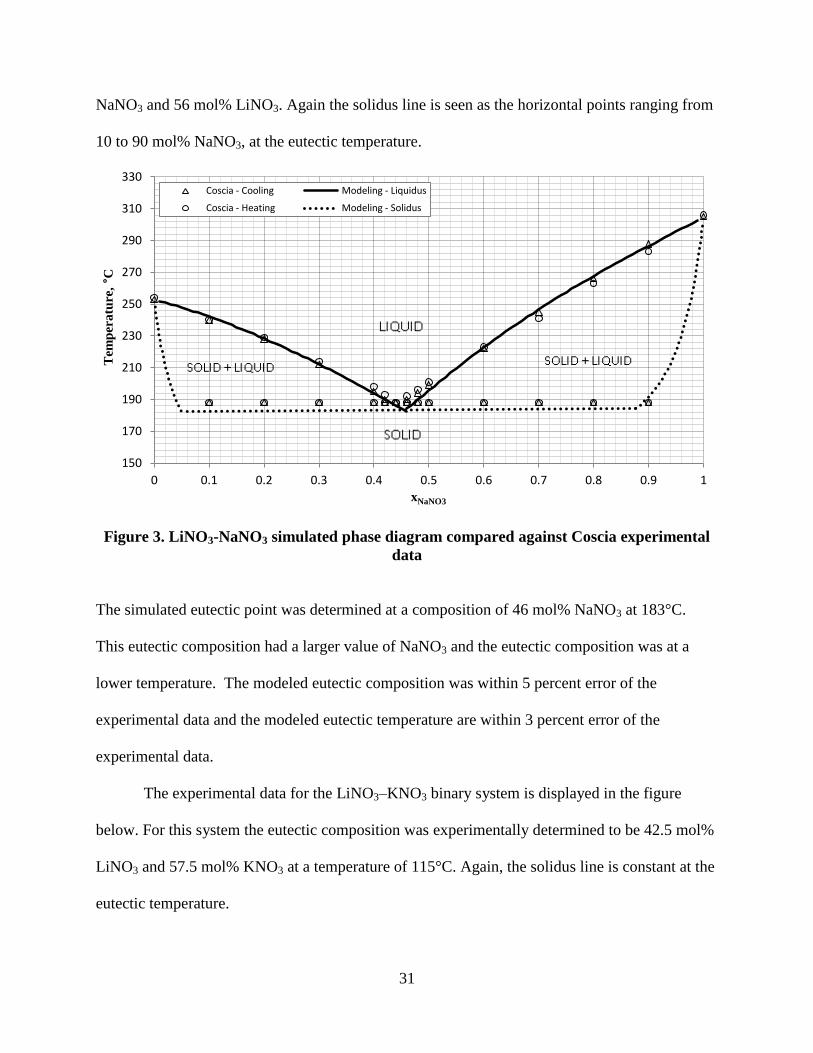
34

Figure 6. LiNO3-NaNO3 simulated phase diagram compared against Campbell and Vallet

experimental data

Our predicted liquidus curve is in very good agreement with both Vallet's and Campbell's

experimental data. There are some minor disagreements with the coordinates of the eutectic

point, however. Vallet's reported the eutectic at 46 mol% NaNO3 agrees with the predictions here

but the temperature is higher than ours. Campbell reported his eutectic at a temperature similar to

ours but at a composition of 41 mol% NaNO3. Vallet did not report solidus data but Campbell's

solidus data matches up very well with our predicted solidus curve. It should be noted that Vallet

and Campbell used constantly mixed systems and observational techniques rather than

differential scanning calorimetry, which may be the reason for the discrepancy in eutectic data.

And finally our simulated LiNO3-KNO3 phase diagram is compared against experimental

data from Vallet [12] and Zhang et al. [10].

150

170

190

210

230

250

270

290

310

330

0 0.1 0.2 0.3 0.4 0.5 0.6 0.7 0.8 0.9 1

Ts,

°C

xNaNO3

Liquidus Temperatures of the LiNa-NO3 System Campbell - Liquidus

Campbell - Solidus

Vallet - Liquidus

35

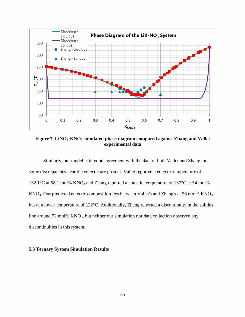
Figure 7. LiNO3-KNO3 simulated phase diagram compared against Zhang and Vallet

experimental data

Similarly, our model is in good agreement with the data of both Vallet and Zhang, but

some discrepancies near the eutectic are present. Vallet reported a eutectic temperature of

132.1°C at 58.1 mol% KNO3 and Zhang reported a eutectic temperature of 137°C at 54 mol%

KNO3. Our predicted eutectic composition lies between Vallet's and Zhang's at 56 mol% KNO3

but at a lower temperature of 122°C. Additionally, Zhang reported a discontinuity in the solidus

line around 52 mol% KNO3, but neither our simulation nor data collection observed any

discontinuities in this system.

5.3 Ternary System Simulation Results

50

100

150

200

250

300

350

0 0.1 0.2 0.3 0.4 0.5 0.6 0.7 0.8 0.9 1

Ts,

°C

xKNO3

Phase Diagram of the LiK-NO3 System Modeling - Liquidus Modeling - Solidus Zhang - Liquidus

Zhang - Solidus

36

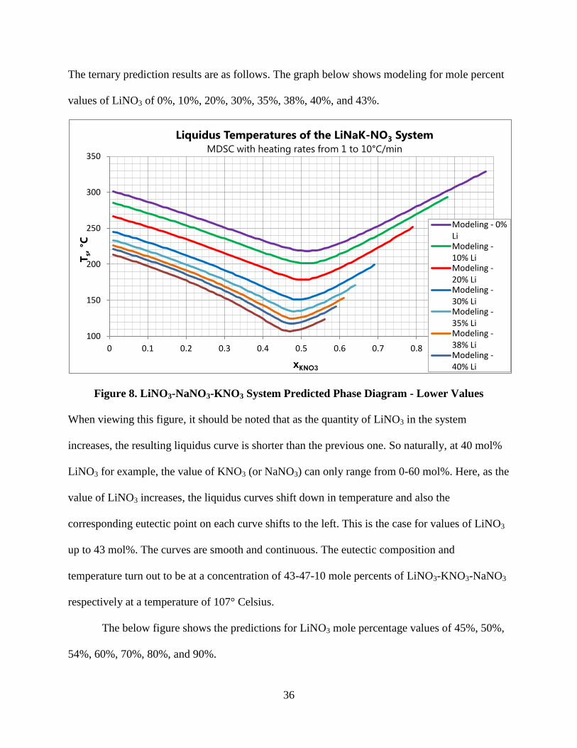
The ternary prediction results are as follows. The graph below shows modeling for mole percent

values of LiNO3 of 0%, 10%, 20%, 30%, 35%, 38%, 40%, and 43%.

Figure 8. LiNO3-NaNO3-KNO3 System Predicted Phase Diagram - Lower Values

When viewing this figure, it should be noted that as the quantity of LiNO3 in the system

increases, the resulting liquidus curve is shorter than the previous one. So naturally, at 40 mol%

LiNO3 for example, the value of KNO3 (or NaNO3) can only range from 0-60 mol%. Here, as the

value of LiNO3 increases, the liquidus curves shift down in temperature and also the

corresponding eutectic point on each curve shifts to the left. This is the case for values of LiNO3

up to 43 mol%. The curves are smooth and continuous. The eutectic composition and

temperature turn out to be at a concentration of 43-47-10 mole percents of LiNO3-KNO3-NaNO3

respectively at a temperature of 107° Celsius.

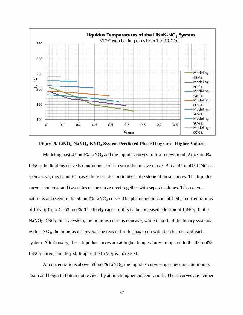
The below figure shows the predictions for LiNO3 mole percentage values of 45%, 50%,

54%, 60%, 70%, 80%, and 90%.

100

150

200

250

300

350

0 0.1 0.2 0.3 0.4 0.5 0.6 0.7 0.8 0.9 1

Ts,

°C

xKNO3

Liquidus Temperatures of the LiNaK-NO3 System

MDSC with heating rates from 1 to 10°C/min

Modeling - 0% Li Modeling - 10% Li Modeling - 20% Li Modeling - 30% Li Modeling - 35% Li Modeling - 38% Li Modeling - 40% Li

37

Figure 9. LiNO3-NaNO3-KNO3 System Predicted Phase Diagram - Higher Values

Modeling past 43 mol% LiNO3 and the liquidus curves follow a new trend. At 43 mol%

LiNO3 the liquidus curve is continuous and is a smooth concave curve. But at 45 mol% LiNO3 as

seen above, this is not the case; there is a discontinuity in the slope of these curves. The liquidus

curve is convex, and two sides of the curve meet together with separate slopes. This convex

nature is also seen in the 50 mol% LiNO3 curve. The phenomenon is identified at concentrations

of LiNO3 from 44-53 mol%. The likely cause of this is the increased addition of LiNO3. In the

NaNO3-KNO3 binary system, the liquidus curve is concave, while in both of the binary systems

with LiNO3, the liquidus is convex. The reason for this has to do with the chemistry of each

system. Additionally, these liquidus curves are at higher temperatures compared to the 43 mol%

LiNO3 curve, and they shift up as the LiNO3 is increased.

At concentrations above 53 mol% LiNO3, the liquidus curve slopes become continuous

again and begin to flatten out, especially at much higher concentrations. These curves are neither

100

150

200

250

300

350

0 0.1 0.2 0.3 0.4 0.5 0.6 0.7 0.8 0.9 1

Ts,

°C

xKNO3

Liquidus Temperatures of the LiNaK-NO3 System

MDSC with heating rates from 1 to 10°C/min

Modeling - 45% Li Modeling - 50% Li Modeling - 54% Li Modeling - 60% Li Modeling - 70% Li Modeling - 80% Li Modeling - 90% Li

38

concave nor complex, but rather they range from the binary temperature at one side of the phase

diagram, to the binary temperature at the other side of the phase diagram. This is more apparent

at higher LiNO3 concentrations namely, the modeling from 60 mol% LiNO3 to 90 mol% LiNO3.

The suspected reason for this is that at these high concentrations, the liquidus curve is equivalent

to one side of the liquidus curve in the corresponding binary system. In the binary systems with

LiNO3, the liquidus curves had to be solved from both sides separately, and the curves here are

simply one of these sides. To ensure the accuracy of these curves the temperature at the end of

each liqudus line was checked against the temperature of the corresponding binary system, which

validated the curves.

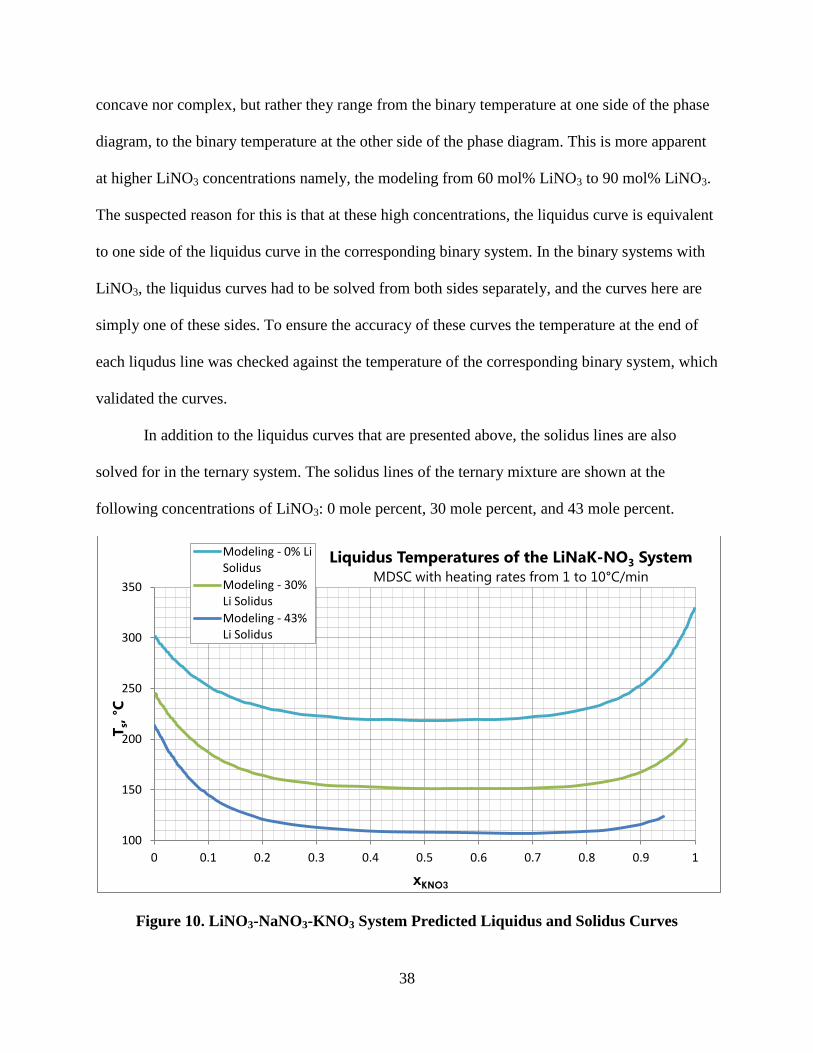
In addition to the liquidus curves that are presented above, the solidus lines are also

solved for in the ternary system. The solidus lines of the ternary mixture are shown at the

following concentrations of LiNO3: 0 mole percent, 30 mole percent, and 43 mole percent.

Figure 10. LiNO3-NaNO3-KNO3 System Predicted Liquidus and Solidus Curves

100

150

200

250

300

350

0 0.1 0.2 0.3 0.4 0.5 0.6 0.7 0.8 0.9 1

Ts,

°C

xKNO3

Liquidus Temperatures of the LiNaK-NO3 System

MDSC with heating rates from 1 to 10°C/min

Modeling - 0% Li Solidus

Modeling - 30% Li Solidus

Modeling - 43% Li Solidus

39

The figure above represent slices of the full ternary system's phase diagram and does not

show the full picture. Because the NaNO3- KNO3- LiNO3 consists of three components, the

complete phase diagram is depicted as a surface plot, and is shown at different views in the

figures below.

Figure 11a. Ternary phase diagram surface plot

40

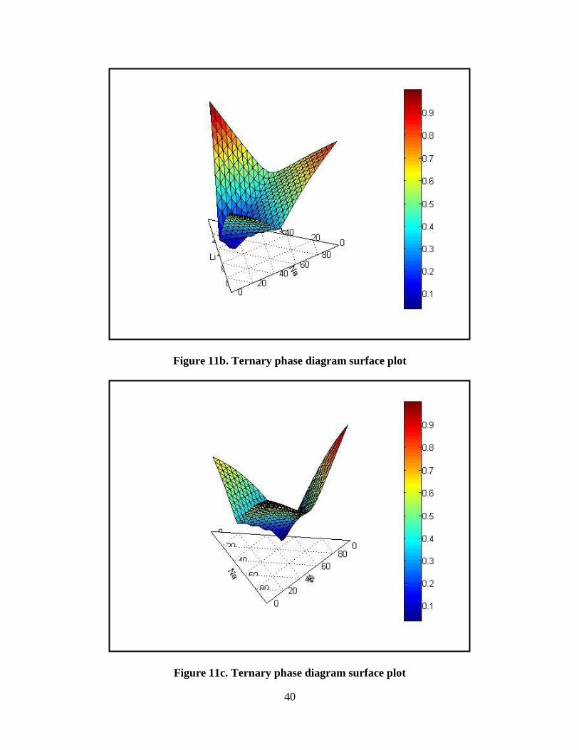
Figure 11b. Ternary phase diagram surface plot

Figure 11c. Ternary phase diagram surface plot

41

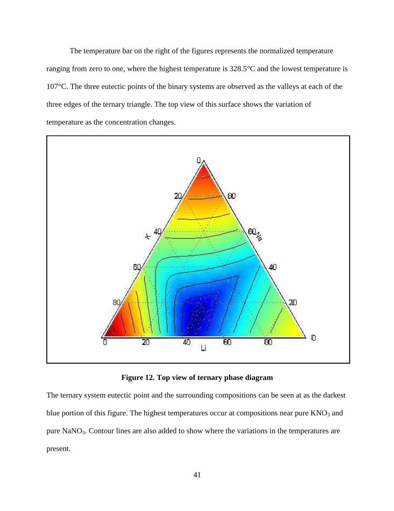
The temperature bar on the right of the figures represents the normalized temperature

ranging from zero to one, where the highest temperature is 328.5°C and the lowest temperature is

107°C. The three eutectic points of the binary systems are observed as the valleys at each of the

three edges of the ternary triangle. The top view of this surface shows the variation of

temperature as the concentration changes.

Figure 12. Top view of ternary phase diagram

The ternary system eutectic point and the surrounding compositions can be seen at as the darkest

blue portion of this figure. The highest temperatures occur at compositions near pure KNO3 and

pure NaNO3. Contour lines are also added to show where the variations in the temperatures are

present.

42

5.4 Ternary System Comparison Results

The ternary prediction results are now compared to experimental data that was collected.

The modeling will be split into separate graphs so the comparison with experimental data will be

easier to observe. First, comparisons at low concentrations of LiNO3, can be seen in the figure

below.

Figure 13. LiNO3-NaNO3-KNO3 simulated phase diagram compared against experimental

data, low LiNO3 values

The predicted values match up well with the experimental data at low concentrations but at

concentrations of 20 and 30 mol% KNO3, a discrepancy is observed near the eutectic points of

the curves. This difference decreases at 35 mol% LiNO3, and at 38 mol% LiNO3 the model and

experimental data match very well, except for a minor disagreement around 40 mol% KNO3.

The next graph shows the model at higher concentrations of LiNO3.

100

150

200

250

300

350

0 0.1 0.2 0.3 0.4 0.5 0.6 0.7 0.8 0.9 1

Ts,

°C

xKNO3

Liquidus Temperatures of the LiNaK-NO3 System

MDSC with heating rates from 1 to 10°C/min

0 mol% LiNO3

10 mol% LiNO3 20 mol% LiNO3 30 mol% LiNO3 35 mol% LiNO3 38 mol% LiNO3 Modeling - 0% Li

43

Figure 14. LiNO3-NaNO3-KNO3 simulated phase diagram compared against experimental

data, eutectic LiNO3 values

The simulations are produced at 40, 43, and 45 mol% LiNO3. First, the modeling at 40

mol% LiNO3 is at temperatures below the experimental data at 38 mol% LiNO3 which is

expected. Modeling the increase in LiNO3 up to 43 mol% follows the same manner, reaching the

eutectic point as described above. And at 45 mol% LiNO3, the discontinuous nature in the slope

of the liquidus curve is observed, which was explained earlier.

The results above give an informative idea to the behavior of these salt mixtures. The

next step would be to use these results and apply them to real-world applications. For instance,

companies who would make use of these molten nitrate salts as heat transfer fluids, this

information can be used to make cost-effective decisions.

Lower melting points, as discussed above, is an important characteristic in heat transfer

fluids for concentrated solar power plants. Using a composition that is not near the eutectic point

100

120

140

160

180

200

220

240

260

280

300

0 0.1 0.2 0.3 0.4 0.5 0.6 0.7 0.8 0.9 1

Ts,

°C

xKNO3

Liquidus Temperatures of the LiNaK-NO3 System

MDSC with heating rates from 1 to 10°C/min

0 mol% LiNO3

10 mol% LiNO3

20 mol% LiNO3

30 mol% LiNO3

35 mol% LiNO3

37 mol% LiNO3

38 mol% LiNO3

Modeling - 43% Li

Modeling - 40% Li

Modeling - 45% Li

44

of a certain system would be a waste of resources for that company. In addition, the cost of each

of these salts are of interest for companies. If the cost of each of these three salts were identical,

obviously choosing the system with the lowest eutectic temperature (the ternary system in this

case), would be the logical choice. But, if one component is more expensive than the others, one

might not just choose the eutectic composition blindly, but might choose a composition that has a

higher melting temperature but less of the more expensive component if this will reduce the cost

for a company in the long run.

45

Chapter 6. Conclusions

The present work illustrates the modeling of phase diagrams of selected binary and

ternary nitrate salts. The results presented validate the use of the Gibbs energy minimization

model used. The phase diagram simulations matched well with the experimental data collected

here and with data gathered by other researchers. For the binary systems, the thermodynamic

model that was used involved setting the liquid and solid phases equal to each other. Because of

this, when solving the resulting equations, both the liquidus and solidus curves were produced.

The same model was used for the ternary system. Here though, only those empirical coefficients

used for each binary mixture were needed to accurately model the ternary phase diagram. This

demonstrates that the binary interactions between the salts have a much larger influence than the

ternary interaction. The equations were solved using a built-in MATLAB solver function, which

simultaneously solves the resulting coupled non-linear set of equations at each inputted

concentration. The eutectic points of each system was determined, with the LiNO3-KNO3 binary

system having the lowest predicted binary temperature of 122° Celsius. The binary simulations

agree very well with the experimental data collected by our group using differential scanning

calorimetry. The predicted ternary eutectic point was determined to be at a composition of 43

mol% LiNO3, 47 mol% KNO3, and 10 mol% NaNO3 with the temperature bring 107° Celsius.

The ternary phase diagram also is in reasonable agreement with the data collected by our group.

It should be noted that the strategy used to model these phase diagrams is not trivial.

Many different methods and procedures exist, some of which were attempted, with less than

satisfactory findings. Using the Gibbs function is a common theme, but in representing the

interactions between the components, numerous approaches exist. Possessing a thermodynamic

46

model which can accurately predict the phase diagrams of binary and ternary mixtures is a

valuable asset to researchers as well as concentrated solar power companies.

47

Chapter 7. Further Research

Further research into the thermodynamic models presented should include treating the

salt's properties such as specific heat and latent heats, not as constants, but as functions of

temperature. This may have the effect of improving the simulations. Another interesting analysis

that could be conducted would be to investigate how changes in the binary coefficients would

affect the ternary phase diagram simulations. For example, choosing coefficients which may not

produce an accurate binary simulation but will better match the ternary experimental data may be

found. Conducting research into the possible effect of the addition of the ternary interaction

between the three components, when modeling the ternary mixture should be done. This was

assumed to be negligible in our models. The addition of other alkali metals should also be

studied, such as rubidium or cesium. Alkaline nitrates could also be included in this research.

Additionally, this thermodynamic model is not unique to nitrate systems, but could also be

applied to other anion systems, for example halides. Use of these different compounds can

provide further verification of the model. Lastly, using this formulation for higher-order systems,

four or five components systems for instance, should be investigated.

48

List of References

1. B. K. Hodge. Alternative Energy Systems and Applications. 2010. John Wiley and Sons Inc.,

Print.

2. Robert W. Bradshaw. Viscosity of Multi-component Molten Nitrate Salts - Liquidus to 200°C.

2010. Sandia National Laboratories, pp. 1-21.

3. M. L. McGlashan. Chemical Thermodynamics. 1979. Academic Press Inc, pp. 268. Print.

4. I. Prigogine, R. Defay. Chemical Thermodynamics. 1973. Longman Group Limited, London,

pp.177-178. Print.

5. C. M. Kramer, C. J. Wilson. The Phase Diagram of NaNO3-KNO3. 1980. Thermochimica

Acta, 42, pp. 253-264.

6. O. J. Kleppa, L.S. Hersh. Heats of Mixing in Liquid Alkali Nitrate Salt Systems. 1961. The

Journal of Chemical Physics, Vol. 34, No. 2, pp. 351-358.

7. P. Jablonski, A. Muller-Blecking, W. Borchard. A Method to Determine Mixing Enthalpies By

DSC. 2003. Journal of Thermal Analysis and Calorimetry, Vol. 74, pp. 779-787.

8. P. J. Spencer. A Brief History of CALPHAD. 2008. Computer Coupling of Phase Diagrams

and Thermochemistry 32, pp. 1-8.

9. O. J. Kleppa, L.S. Hersh. Calorimetry in Liquid Thallium Nitrate-Alkali Nitrate Mixtures.

1962. The Journal of Chemical Physics, Vol. 36, No. 2, pp. 544-547.

10. Xuejun Zhang, Kangcheng Xu, Yici Gao. The Phase Diagram of LiNO3-KNO3. 2002.

Thermochimica Acta, 385, pp. 81-84.

11. Xuejun Zhang, Jun Tian, Kangcheng Xu, Yici Gao. Thermodynamic Evaluation of Phase

Equilibria in NaNO3-KNO3 System. 2003. Journal of Phase Equilibria, Vol. 24, No. 5, 441-446.

49

12. A. N. Campbell, E. M. Kartzmark, M. K. Nagarajan. The Binary (Anhydrous) Systems of

NaNO3-LiNO3, LiClO3-NaClO3, LiClO3-LiNO3, NaNO3-NaClO3 and the Quaternary System of

NaNO3- LiNO3-LiClO3-NaClO3. 1962. Canadian Journal of Chemistry, 40, pp. 1258-1265.

13. C. Vallet. Phase Diagrams and Thermodynamic Properties of some Molten Nitrate Mixtures.

1972. Journal of Chemical Thermodynamics, 4, pp. 105-114.

14. A. G. Bergman, K. Nogoev. The CO(NH2)2-LiNO3; K, Li, Na || NO3; and K, NH4, Na || NO3

Systems. 1964. Russian Journal of Inorganic Chemistry, Vol. 9, No. 6, 771-773.

15. K. Coscia, S. Nelle, T. Elliott, S. Mohapatra, A. Oztekin, S. Neti. The Thermophysical

Properties of the Na-K, Li-Na, and Li-K Nitrate Salt Systems. 2011. ASME Conference IMECE

16. K. Coscia, S. Nelle, T. Elliott, S. Mohapatra, A. Oztekin, S. Neti. The Heat Transfer

Characteristics and Phase Diagram Modeling of Molten Binary Nitrate Salt System. 2011.

SolarPACES Conference.

17. Y. Takahashi, R. Sakamoto, M. Kamimoto. Heat Capacities and Latent Heats of LiNO3,

NaNO3, KNO3. 1988. International Journal of Thermophysics, Vol. 9, No. 6, 1081-1090.

18. M. J. Maeso and J. Largo. Phase Diagrams of LiNO3-KNO3 and LiNO3-KNO3: the

Behaviour of Liquid Mixtures. 1993. Thermochimica Acta, 223, pp. 145-156.

19. The Mathworks, Inc. Equation Solving Algorithms.

http://www.mathworks.com/help/toolbox/optim/ug/brnoyhf.html

50

Vita

Tucker is the son of Walter T. and PattiAnn Elliott and was born on March 18, 1988. He

grew up in Huntington, New York. He received his Bachelor of Science in mechanical

engineering with high honors from Lehigh University in May of 2010. As a presidential scholar,

he continued his education at Lehigh, and will receive his Master of Science in mechanical

engineering in January of 2012.