gilberto a. paula - ime-uspgiapaula/slides_exemplos_semip.pdf · semiparametric models with...
TRANSCRIPT

Semiparametric models with applications using R
Gilberto A. Paula
Instituto de Matemática e EstatísticaUniversidade de São Paulo, Brasil
2o Semestre 2016
G. A. Paula (IME-USP) Semiparametric models in R 2o Semestre 2016 1 / 61

Examples
Outline
1 Examples
2 Defining f (x)
3 Additive normal model
4 Semiparametric normal model
5 Packages in R
6 Voltage drop data
7 Boston housing data
8 Bibliography
G. A. Paula (IME-USP) Semiparametric models in R 2o Semestre 2016 2 / 61

Examples
Voltage drop data
Description
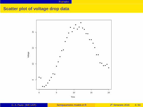
As a 1st example we will consider the voltage drop data (Montgomeryand Peck, 2001) in which a battery voltage drop in a guided missilemotor is observed over the time of missile flight. It was intended avoltage drop model for using a digital-analog simulation model of themissile. Altogether there are 41 observations.
G. A. Paula (IME-USP) Semiparametric models in R 2o Semestre 2016 3 / 61
Examples
Scatter plot of voltage drop data
0 5 10 15 20
810
1214
Time
Volta
ge
G. A. Paula (IME-USP) Semiparametric models in R 2o Semestre 2016 4 / 61

Examples
Scatter plot of voltage drop data
0 5 10 15 20
810
1214
Time
Volta
ge
G. A. Paula (IME-USP) Semiparametric models in R 2o Semestre 2016 5 / 61

Examples
Possible model
Description
The data suggest a nonparametric model such as:
Voltagei = α+ f (Timei) + ǫi ,
G. A. Paula (IME-USP) Semiparametric models in R 2o Semestre 2016 6 / 61

Examples
Possible model
Description
The data suggest a nonparametric model such as:
Voltagei = α+ f (Timei) + ǫi ,
where ǫi∼ N(0, σ2) for i = 1, . . . , 41, with f (·) being a continuous,smooth and nonparametric function.
G. A. Paula (IME-USP) Semiparametric models in R 2o Semestre 2016 6 / 61

Examples
Boston housing data
Description
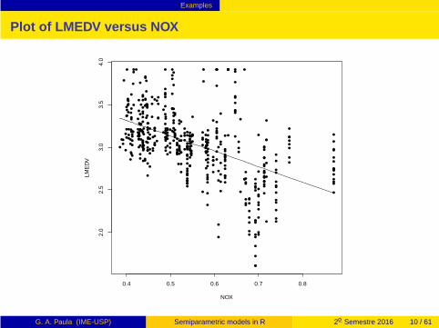
As a 2nd example we will consider the Boston housing data that havebeen analyzed by various authors (see, for instance, Belsley et al.1980). The aim of the study is to assess the association of houseprices with the air quality of the neighborhood by using regressionmodels. The outcome variable
G. A. Paula (IME-USP) Semiparametric models in R 2o Semestre 2016 7 / 61

Examples
Boston housing data
Description
As a 2nd example we will consider the Boston housing data that havebeen analyzed by various authors (see, for instance, Belsley et al.1980). The aim of the study is to assess the association of houseprices with the air quality of the neighborhood by using regressionmodels. The outcome variable
LMEDV (logarithm of the median house price in USD 1000)
is related with 13 explanatory variables. Altogether there are 506observations.
G. A. Paula (IME-USP) Semiparametric models in R 2o Semestre 2016 7 / 61

Examples
Boston housing data
Illustration
We will work, for the purpose of motivating the semi-parametricmodels, with three explanatory variables:
G. A. Paula (IME-USP) Semiparametric models in R 2o Semestre 2016 8 / 61

Examples
Boston housing data
Illustration
We will work, for the purpose of motivating the semi-parametricmodels, with three explanatory variables:
NOX (annual average nitric oxide concentration, p.p. 10 million);
G. A. Paula (IME-USP) Semiparametric models in R 2o Semestre 2016 8 / 61

Examples
Boston housing data
Illustration
We will work, for the purpose of motivating the semi-parametricmodels, with three explanatory variables:
NOX (annual average nitric oxide concentration, p.p. 10 million);
LSTAT (% lower status of the population);
DIS (weighted distances to five Boston employment centers).
G. A. Paula (IME-USP) Semiparametric models in R 2o Semestre 2016 8 / 61

Examples
Plot of LMEDV versus NOX
0.4 0.5 0.6 0.7 0.8
2.0
2.5
3.0
3.5
4.0
NOX
LME
DV
G. A. Paula (IME-USP) Semiparametric models in R 2o Semestre 2016 9 / 61
Examples
Plot of LMEDV versus NOX
0.4 0.5 0.6 0.7 0.8
2.0
2.5
3.0
3.5
4.0
NOX
LME
DV
G. A. Paula (IME-USP) Semiparametric models in R 2o Semestre 2016 10 / 61

Examples
Plot of LMEDV versus LSTAT
10 20 30
2.0
2.5
3.0
3.5
4.0
LSTAT
LME
DV
G. A. Paula (IME-USP) Semiparametric models in R 2o Semestre 2016 11 / 61

Examples
Plot of LMEDV versus LSTAT
10 20 30
2.0
2.5
3.0
3.5
4.0
LSTAT
LME
DV
G. A. Paula (IME-USP) Semiparametric models in R 2o Semestre 2016 12 / 61

Examples
Plot of LMEDV versus DIS
2 4 6 8 10 12
2.0
2.5
3.0
3.5
4.0
DIS
LME
DV
G. A. Paula (IME-USP) Semiparametric models in R 2o Semestre 2016 13 / 61

Examples
Plot of LMEDV versus DIS
2 4 6 8 10 12
2.0
2.5
3.0
3.5
4.0
DIS
LME
DV
G. A. Paula (IME-USP) Semiparametric models in R 2o Semestre 2016 14 / 61

Examples
Possible model
Description
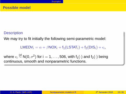
We may try to fit initially the following semi-parametric model:
LMEDVi = α+ βNOXi + f1(LSTATi) + f2(DISi) + ǫi ,
G. A. Paula (IME-USP) Semiparametric models in R 2o Semestre 2016 15 / 61
Examples
Possible model
Description
We may try to fit initially the following semi-parametric model:
LMEDVi = α+ βNOXi + f1(LSTATi) + f2(DISi) + ǫi ,
where ǫiiid∼ N(0, σ2) for i = 1, . . . , 506, with f1(·) and f2(·) being
continuous, smooth and nonparametric functions.
G. A. Paula (IME-USP) Semiparametric models in R 2o Semestre 2016 15 / 61

Examples
Comparison of snacks
Description
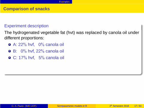
As a 3rd example, we will consider a data set from an experimentdeveloped in School of Public Health - Universidade de São Paulo, inwhich 4 different forms of light snacks (B, C, D and E) were comparedacross 20 weeks with a traditional snack (A).
G. A. Paula (IME-USP) Semiparametric models in R 2o Semestre 2016 16 / 61

Examples
Comparison of snacks
Experiment description
The hydrogenated vegetable fat (hvt) was replaced by canola oil underdifferent proportions:
G. A. Paula (IME-USP) Semiparametric models in R 2o Semestre 2016 17 / 61

Examples
Comparison of snacks
Experiment description
The hydrogenated vegetable fat (hvt) was replaced by canola oil underdifferent proportions:
A: 22% hvf, 0% canola oil
G. A. Paula (IME-USP) Semiparametric models in R 2o Semestre 2016 17 / 61

Examples
Comparison of snacks
Experiment description
The hydrogenated vegetable fat (hvt) was replaced by canola oil underdifferent proportions:
A: 22% hvf, 0% canola oil
B: 0% hvf, 22% canola oil
G. A. Paula (IME-USP) Semiparametric models in R 2o Semestre 2016 17 / 61
Examples
Comparison of snacks
Experiment description
The hydrogenated vegetable fat (hvt) was replaced by canola oil underdifferent proportions:
A: 22% hvf, 0% canola oil
B: 0% hvf, 22% canola oil
C: 17% hvf, 5% canola oil
G. A. Paula (IME-USP) Semiparametric models in R 2o Semestre 2016 17 / 61

Examples
Comparison of snacks
Experiment description
The hydrogenated vegetable fat (hvt) was replaced by canola oil underdifferent proportions:
A: 22% hvf, 0% canola oil
B: 0% hvf, 22% canola oil
C: 17% hvf, 5% canola oil
D: 11% hvf, 11% canola oil
E: 5% hvf, 17% canola oil.
In this analysis we will only consider the variable TEXTURE that will becompared across time among the 5 snack types.
G. A. Paula (IME-USP) Semiparametric models in R 2o Semestre 2016 17 / 61

Examples
Mean profiles
5 10 15 20
4050
6070
80
Weeks
Text
ure
ABCDE
G. A. Paula (IME-USP) Semiparametric models in R 2o Semestre 2016 18 / 61

Examples
Variation coefficient profiles
5 10 15 20
0.05
0.10
0.15
0.20
0.25
0.30
0.35
Weeks
VC
of T
extu
reABCDE
G. A. Paula (IME-USP) Semiparametric models in R 2o Semestre 2016 19 / 61

Examples
Double gamma model
Description
Similarly to Paula (2013) we may consider a semi-parametric doublegamma model:
G. A. Paula (IME-USP) Semiparametric models in R 2o Semestre 2016 20 / 61

Examples
Double gamma model
Description
Similarly to Paula (2013) we may consider a semi-parametric doublegamma model:
yijkind∼ G(µij , φij);
G. A. Paula (IME-USP) Semiparametric models in R 2o Semestre 2016 20 / 61

Examples
Double gamma model
Description
Similarly to Paula (2013) we may consider a semi-parametric doublegamma model:
yijkind∼ G(µij , φij);
log(µij) = β0 + βi + f (Weeksj);
G. A. Paula (IME-USP) Semiparametric models in R 2o Semestre 2016 20 / 61

Examples
Double gamma model
Description
Similarly to Paula (2013) we may consider a semi-parametric doublegamma model:
yijkind∼ G(µij , φij);
log(µij) = β0 + βi + f (Weeksj);
log(φ−1ij ) = γ0 + γi ,
G. A. Paula (IME-USP) Semiparametric models in R 2o Semestre 2016 20 / 61

Examples
Double gamma model
Description
Similarly to Paula (2013) we may consider a semi-parametric doublegamma model:
yijkind∼ G(µij , φij);
log(µij) = β0 + βi + f (Weeksj);
log(φ−1ij ) = γ0 + γi ,
for i = 1(A), 2(B), 3(C), 4(D), 5(E), j = 2, 4, . . . , 20 and k = 1, . . . , 15,where φ−1
ij is the dispersion parameter, β0 + βi and γ0 + γi denote thesnack effects whereas f (·) is continuous, smooth and nonparametricfunction.
G. A. Paula (IME-USP) Semiparametric models in R 2o Semestre 2016 20 / 61

Defining f (x)
Outline
1 Examples
2 Defining f (x)
3 Additive normal model
4 Semiparametric normal model
5 Packages in R
6 Voltage drop data
7 Boston housing data
8 Bibliography
G. A. Paula (IME-USP) Semiparametric models in R 2o Semestre 2016 21 / 61

Defining f (x)
Defining f (x)
How to define f (x)?
G. A. Paula (IME-USP) Semiparametric models in R 2o Semestre 2016 22 / 61

Defining f (x)
Defining f (x)
How to define f (x)?
Piecewise-cubic splines
G. A. Paula (IME-USP) Semiparametric models in R 2o Semestre 2016 22 / 61

Defining f (x)
Defining f (x)
How to define f (x)?
Piecewise-cubic splinesB-splines
G. A. Paula (IME-USP) Semiparametric models in R 2o Semestre 2016 22 / 61

Defining f (x)
Defining f (x)
How to define f (x)?
Piecewise-cubic splinesB-splines
Natural cubic splines
G. A. Paula (IME-USP) Semiparametric models in R 2o Semestre 2016 22 / 61

Defining f (x)
Defining f (x)
How to define f (x)?
Piecewise-cubic splinesB-splines
Natural cubic splinesP-splines
G. A. Paula (IME-USP) Semiparametric models in R 2o Semestre 2016 22 / 61

Defining f (x)
Defining f (x)
How to define f (x)?
Piecewise-cubic splinesB-splines
Natural cubic splinesP-splinesThin-plate splines
G. A. Paula (IME-USP) Semiparametric models in R 2o Semestre 2016 22 / 61

Defining f (x)
Defining f (x)
How to define f (x)?
Piecewise-cubic splinesB-splines
Natural cubic splinesP-splinesThin-plate splines· · ·
G. A. Paula (IME-USP) Semiparametric models in R 2o Semestre 2016 22 / 61

Defining f (x)
Defining f (x)
How to define f (x)?
Piecewise-cubic splinesB-splines
Natural cubic splinesP-splinesThin-plate splines· · ·
Kernel
G. A. Paula (IME-USP) Semiparametric models in R 2o Semestre 2016 22 / 61

Defining f (x)
Defining f (x)
How to define f (x)?
Piecewise-cubic splinesB-splines
Natural cubic splinesP-splinesThin-plate splines· · ·
Kernel
Loess
G. A. Paula (IME-USP) Semiparametric models in R 2o Semestre 2016 22 / 61

Defining f (x)
Defining f (x)
How to define f (x)?
Piecewise-cubic splinesB-splines
Natural cubic splinesP-splinesThin-plate splines· · ·
Kernel
Loess
Wavelets
G. A. Paula (IME-USP) Semiparametric models in R 2o Semestre 2016 22 / 61

Defining f (x)
Defining f (x)
How to define f (x)?
Piecewise-cubic splinesB-splines
Natural cubic splinesP-splinesThin-plate splines· · ·
Kernel
Loess
Wavelets
· · ·
G. A. Paula (IME-USP) Semiparametric models in R 2o Semestre 2016 22 / 61

Defining f (x)
Piecewise-cubic splines
Definition
Suppose the explanatory variable values are in the interval [a, b], fori = 1, . . . , n, with m internal knots, namely a < t1 < · · · < tm < b,where m ≤ n − 2.
G. A. Paula (IME-USP) Semiparametric models in R 2o Semestre 2016 23 / 61

Defining f (x)
Piecewise-cubic splines
Definition
Suppose the explanatory variable values are in the interval [a, b], fori = 1, . . . , n, with m internal knots, namely a < t1 < · · · < tm < b,where m ≤ n − 2.
A simple choice for the nonparametric function f (x) could be thepiecewise-cubic spline, described as
f (x) = β0 + β1x + β2x2 +
m∑
j=1
γj(x − tj)3+,
where
(x − tj)+ =
{
0 se x ≤ tj(x − tj) se x > tj ,
G. A. Paula (IME-USP) Semiparametric models in R 2o Semestre 2016 23 / 61

Defining f (x)
Voltage drop data
Suppose m = 2 internal knots at t1 = 6.5 and t2 = 13.
G. A. Paula (IME-USP) Semiparametric models in R 2o Semestre 2016 24 / 61

Defining f (x)
Voltage drop data
Suppose m = 2 internal knots at t1 = 6.5 and t2 = 13.
0 5 10 15 20
810
1214
Time
Volta
ge
G. A. Paula (IME-USP) Semiparametric models in R 2o Semestre 2016 24 / 61

Defining f (x)
Voltage drop data
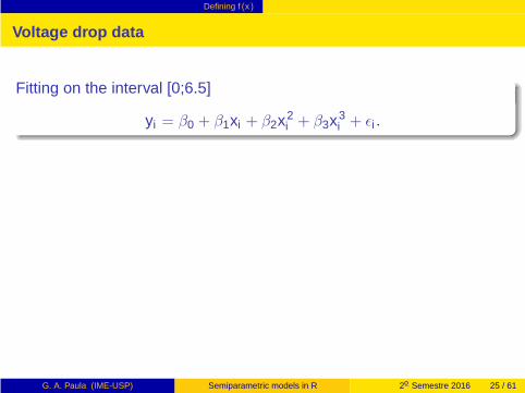
Fitting on the interval [0;6.5]
G. A. Paula (IME-USP) Semiparametric models in R 2o Semestre 2016 25 / 61
Defining f (x)
Voltage drop data
Fitting on the interval [0;6.5]
yi = β0 + β1xi + β2x2i + β3x3
i + ǫi .
G. A. Paula (IME-USP) Semiparametric models in R 2o Semestre 2016 25 / 61

Defining f (x)
Voltage drop data
Fitting on the interval [0;6.5]
yi = β0 + β1xi + β2x2i + β3x3
i + ǫi .
Fitting on the interval (6.5;13]
G. A. Paula (IME-USP) Semiparametric models in R 2o Semestre 2016 25 / 61

Defining f (x)
Voltage drop data
Fitting on the interval [0;6.5]
yi = β0 + β1xi + β2x2i + β3x3
i + ǫi .
Fitting on the interval (6.5;13]
yi = β0 + β1xi + β2x2i + β3x3
i + γ1(xi − 6.5)3 + ǫi .
G. A. Paula (IME-USP) Semiparametric models in R 2o Semestre 2016 25 / 61

Defining f (x)
Voltage drop data
Fitting on the interval [0;6.5]
yi = β0 + β1xi + β2x2i + β3x3
i + ǫi .
Fitting on the interval (6.5;13]
yi = β0 + β1xi + β2x2i + β3x3
i + γ1(xi − 6.5)3 + ǫi .
Fitting on the interval (13;20]
G. A. Paula (IME-USP) Semiparametric models in R 2o Semestre 2016 25 / 61

Defining f (x)
Voltage drop data
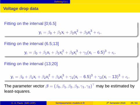
Fitting on the interval [0;6.5]
yi = β0 + β1xi + β2x2i + β3x3
i + ǫi .
Fitting on the interval (6.5;13]
yi = β0 + β1xi + β2x2i + β3x3
i + γ1(xi − 6.5)3 + ǫi .
Fitting on the interval (13;20]
yi = β0 + β1xi + β2x2i + β3x3
i + γ1(xi − 6.5)3 + γ2(xi − 13)3 + ǫi .
G. A. Paula (IME-USP) Semiparametric models in R 2o Semestre 2016 25 / 61
Defining f (x)
Voltage drop data
Fitting on the interval [0;6.5]
yi = β0 + β1xi + β2x2i + β3x3
i + ǫi .
Fitting on the interval (6.5;13]
yi = β0 + β1xi + β2x2i + β3x3
i + γ1(xi − 6.5)3 + ǫi .
Fitting on the interval (13;20]
yi = β0 + β1xi + β2x2i + β3x3
i + γ1(xi − 6.5)3 + γ2(xi − 13)3 + ǫi .
The parameter vector β = (β0, β1, β2, β3, γ1, γ2)⊤ may be estimated by
least-squares.
G. A. Paula (IME-USP) Semiparametric models in R 2o Semestre 2016 25 / 61

Defining f (x)
B-splines
Definition
A more flexible class that contains candidates for f (x) is the B-splinesclass, defined as
G. A. Paula (IME-USP) Semiparametric models in R 2o Semestre 2016 26 / 61

Defining f (x)
B-splines
Definition
A more flexible class that contains candidates for f (x) is the B-splinesclass, defined as
f (x) =q
∑
j=1
Nj(x)τj , x ∈ [a, b],
G. A. Paula (IME-USP) Semiparametric models in R 2o Semestre 2016 26 / 61

Defining f (x)
B-splines
Definition
A more flexible class that contains candidates for f (x) is the B-splinesclass, defined as
f (x) =q
∑
j=1
Nj(x)τj , x ∈ [a, b],
where Nj(x) are the B-spline basis functions and τj are coefficients.
G. A. Paula (IME-USP) Semiparametric models in R 2o Semestre 2016 26 / 61

Defining f (x)
Natural cubic splines
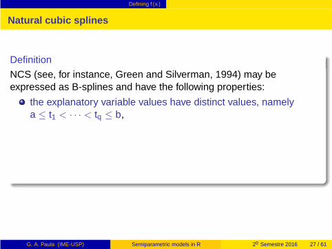
Definition
NCS (see, for instance, Green and Silverman, 1994) may beexpressed as B-splines and have the following properties:
G. A. Paula (IME-USP) Semiparametric models in R 2o Semestre 2016 27 / 61
Defining f (x)
Natural cubic splines
Definition
NCS (see, for instance, Green and Silverman, 1994) may beexpressed as B-splines and have the following properties:
the explanatory variable values have distinct values, namelya ≤ t1 < · · · < tq ≤ b,
G. A. Paula (IME-USP) Semiparametric models in R 2o Semestre 2016 27 / 61

Defining f (x)
Natural cubic splines
Definition
NCS (see, for instance, Green and Silverman, 1994) may beexpressed as B-splines and have the following properties:
the explanatory variable values have distinct values, namelya ≤ t1 < · · · < tq ≤ b,
f (x) is a cubic spline in the intervals [t1, t2], . . . , [tq−1, tq],
f (x) is linear in the intervals [a, t1] and [tq, b],
f (x), f ′(x) and f ′′(x) are continuous.
Therefore, for NCS one has m = q − 2 internal knots.
NCS may also be defined for arbitrary m internal knots.
G. A. Paula (IME-USP) Semiparametric models in R 2o Semestre 2016 27 / 61

Defining f (x)
P-splines
Definition
P-splines (Eilers and Marx, 1996) form a flexible class of B-splinesdefined as
G. A. Paula (IME-USP) Semiparametric models in R 2o Semestre 2016 28 / 61

Defining f (x)
P-splines
Definition
P-splines (Eilers and Marx, 1996) form a flexible class of B-splinesdefined as
f (x) =q
∑
j=1
Nj,k (x)τj , x ∈ [a, b],
G. A. Paula (IME-USP) Semiparametric models in R 2o Semestre 2016 28 / 61

Defining f (x)
P-splines
Definition
P-splines (Eilers and Marx, 1996) form a flexible class of B-splinesdefined as
f (x) =q
∑
j=1
Nj,k (x)τj , x ∈ [a, b],
where Nj,k (x) are the B-spline basis functions of degree k (de Boor,1978), for k = 0, 1, 2, . . ., τj are coefficients, m is the number of internalknots, namely a < t1 < · · · < tm < b, and m = q + k + 1.
G. A. Paula (IME-USP) Semiparametric models in R 2o Semestre 2016 28 / 61

Defining f (x)
P-splines
Basis function
De Boor’s B-splines basis functions are expressed as
G. A. Paula (IME-USP) Semiparametric models in R 2o Semestre 2016 29 / 61

Defining f (x)
P-splines
Basis function
De Boor’s B-splines basis functions are expressed as
Nj,0(x) ={
1 tj ≤ x ≤ tj+1
0 otherwise
G. A. Paula (IME-USP) Semiparametric models in R 2o Semestre 2016 29 / 61

Defining f (x)
P-splines
Basis function
De Boor’s B-splines basis functions are expressed as
Nj,0(x) ={
1 tj ≤ x ≤ tj+1
0 otherwise
and
Nj,k (x) =(x − tj)(tj+k − tj)
Nj,k−1(x) +(tj+k+1 − x)(tj+k+1 − tj+1)
Nj+1,k−1(x),
for j = 1, . . . , q and k = 1, 2, 3, . . . .
G. A. Paula (IME-USP) Semiparametric models in R 2o Semestre 2016 29 / 61

Defining f (x)
Penalization
Why to penalize?
The aim of penalization is to reduce the parametric space solution inorder to avoid overfitting.
G. A. Paula (IME-USP) Semiparametric models in R 2o Semestre 2016 30 / 61

Additive normal model
Outline
1 Examples
2 Defining f (x)
3 Additive normal model
4 Semiparametric normal model
5 Packages in R
6 Voltage drop data
7 Boston housing data
8 Bibliography
G. A. Paula (IME-USP) Semiparametric models in R 2o Semestre 2016 31 / 61

Additive normal model
Additive normal model
Description
First, we will assume the following nonparametric model:
G. A. Paula (IME-USP) Semiparametric models in R 2o Semestre 2016 32 / 61

Additive normal model
Additive normal model
Description
First, we will assume the following nonparametric model:
yi = f (ti) + ǫi ,
G. A. Paula (IME-USP) Semiparametric models in R 2o Semestre 2016 32 / 61

Additive normal model
Additive normal model
Description
First, we will assume the following nonparametric model:
yi = f (ti) + ǫi ,
where f (t) is a continuous, smooth and nonparametric function and
ǫiiid∼ N(0, σ2), for i = 1, . . . , n.
G. A. Paula (IME-USP) Semiparametric models in R 2o Semestre 2016 32 / 61

Additive normal model
Additive normal model
Penalization
A suggestion is to use the second derivative penalization.
G. A. Paula (IME-USP) Semiparametric models in R 2o Semestre 2016 33 / 61

Additive normal model
Additive normal model
Penalization
A suggestion is to use the second derivative penalization. So, theobjective function to be minimized is given by
G. A. Paula (IME-USP) Semiparametric models in R 2o Semestre 2016 33 / 61

Additive normal model
Additive normal model
Penalization
A suggestion is to use the second derivative penalization. So, theobjective function to be minimized is given by
SP(f, λ) =n
∑
i=1
{yi − f (ti)}2 + λ
∫ b
a[f ′′(x)]2dx ,
where f = (f (t1), . . . , f (tq))⊤, [a, b] denotes the data interval and λ > 0is the smoothing parameter.
The solution is a natural cubic spline with knots at the distinct valuesa ≤ t1 < · · · < tq ≤ b.
G. A. Paula (IME-USP) Semiparametric models in R 2o Semestre 2016 33 / 61

Additive normal model
Additive normal model
Smoothing parameter
One has the following λ interpretation:
G. A. Paula (IME-USP) Semiparametric models in R 2o Semestre 2016 34 / 61

Additive normal model
Additive normal model
Smoothing parameter
One has the following λ interpretation:
when λ → 0 minimizing SP(f, λ) leads to a data interpolation;
G. A. Paula (IME-USP) Semiparametric models in R 2o Semestre 2016 34 / 61

Additive normal model
Additive normal model
Smoothing parameter
One has the following λ interpretation:
when λ → 0 minimizing SP(f, λ) leads to a data interpolation;
when λ → ∞ one has to impose f ′′(x) = 0 so the solution leads toa linear function for f (x);
then 0 < λ < ∞.
G. A. Paula (IME-USP) Semiparametric models in R 2o Semestre 2016 34 / 61

Additive normal model
Semiparametric normal model
Penalization
One has for B-splines the following solution (see, for instance, Wood,2006):
G. A. Paula (IME-USP) Semiparametric models in R 2o Semestre 2016 35 / 61

Additive normal model
Semiparametric normal model
Penalization
One has for B-splines the following solution (see, for instance, Wood,2006):
∫ b
a[f ′′(x)]2dx = τ⊤Kτ ,
G. A. Paula (IME-USP) Semiparametric models in R 2o Semestre 2016 35 / 61

Additive normal model
Semiparametric normal model
Penalization
One has for B-splines the following solution (see, for instance, Wood,2006):
∫ b
a[f ′′(x)]2dx = τ⊤Kτ ,
where K is a (q × q) non-negative definite smoothing matrix that doesnot depend on τ .
G. A. Paula (IME-USP) Semiparametric models in R 2o Semestre 2016 35 / 61

Semiparametric normal model
Outline
1 Examples
2 Defining f (x)
3 Additive normal model
4 Semiparametric normal model
5 Packages in R
6 Voltage drop data
7 Boston housing data
8 Bibliography
G. A. Paula (IME-USP) Semiparametric models in R 2o Semestre 2016 36 / 61

Semiparametric normal model
Semiparametric normal model
Description
We will assume now the following partially linear model:
G. A. Paula (IME-USP) Semiparametric models in R 2o Semestre 2016 37 / 61

Semiparametric normal model
Semiparametric normal model
Description
We will assume now the following partially linear model:
yi = x⊤
i β + f (ti) + ǫi ,
G. A. Paula (IME-USP) Semiparametric models in R 2o Semestre 2016 37 / 61

Semiparametric normal model
Semiparametric normal model
Description
We will assume now the following partially linear model:
yi = x⊤
i β + f (ti) + ǫi ,
where x i = (xi1, . . . , xip)⊤ contains values of explanatory variables,
β = (β1, . . . , βp)⊤, f (ti) = N⊤
i τ is a B-spline and ǫiiid∼ N(0, σ2), for
i = 1, . . . , n.
Objective function
The penalized least-squares function becomes
SP(θ, λ) = (y − Xβ − Nτ )⊤(y − Xβ − Nτ ) + λτ⊤Kτ ,
where θ = (β⊤, τ⊤)⊤.
G. A. Paula (IME-USP) Semiparametric models in R 2o Semestre 2016 37 / 61

Semiparametric normal model
Semiparametric normal model
Iterative process
One has the following iterative process:
G. A. Paula (IME-USP) Semiparametric models in R 2o Semestre 2016 38 / 61

Semiparametric normal model
Semiparametric normal model
Iterative process
One has the following iterative process:
starting with β(0) as the parametric least-squares solution;
G. A. Paula (IME-USP) Semiparametric models in R 2o Semestre 2016 38 / 61

Semiparametric normal model
Semiparametric normal model
Iterative process
One has the following iterative process:
starting with β(0) as the parametric least-squares solution;
τ (0) = (N⊤N + λK)−1N⊤(y − Xβ(0));
G. A. Paula (IME-USP) Semiparametric models in R 2o Semestre 2016 38 / 61

Semiparametric normal model
Semiparametric normal model
Iterative process
One has the following iterative process:
starting with β(0) as the parametric least-squares solution;
τ (0) = (N⊤N + λK)−1N⊤(y − Xβ(0));back-fitting (Gauss-Seidel) algorithm:
β(m+1) = (X⊤X)−1X⊤{y − Nτ (m)}
τ (m+1) = (N⊤N + λK)−1N⊤{y − Xβ(m+1)},
for m = 0, 1, 2, . . . and λ fixed.
G. A. Paula (IME-USP) Semiparametric models in R 2o Semestre 2016 38 / 61

Semiparametric normal model
Semiparametric normal model
Effective degrees of freedom
From the iterative process at the convergence one has that
G. A. Paula (IME-USP) Semiparametric models in R 2o Semestre 2016 39 / 61

Semiparametric normal model
Semiparametric normal model
Effective degrees of freedom
From the iterative process at the convergence one has that
f = Nτ
G. A. Paula (IME-USP) Semiparametric models in R 2o Semestre 2016 39 / 61

Semiparametric normal model
Semiparametric normal model
Effective degrees of freedom
From the iterative process at the convergence one has that
f = Nτ
= N(N⊤N + λK)−1N⊤{y − Xβ}
G. A. Paula (IME-USP) Semiparametric models in R 2o Semestre 2016 39 / 61

Semiparametric normal model
Semiparametric normal model
Effective degrees of freedom
From the iterative process at the convergence one has that
f = Nτ
= N(N⊤N + λK)−1N⊤{y − Xβ}
= H(λ){y − Xβ}.
G. A. Paula (IME-USP) Semiparametric models in R 2o Semestre 2016 39 / 61

Semiparametric normal model
Semiparametric normal model
Effective degrees of freedom
From the iterative process at the convergence one has that
f = Nτ
= N(N⊤N + λK)−1N⊤{y − Xβ}
= H(λ){y − Xβ}.
So, as suggested by Hastie and Tibshirani (1990) one may take
df(λ) = tr{H(λ)}
= tr{N(N⊤N + λK)−1N⊤}
= tr{N⊤N(N⊤N + λK)−1}.
G. A. Paula (IME-USP) Semiparametric models in R 2o Semestre 2016 39 / 61

Semiparametric normal model
Semiparametric normal model
Model selection
The Akaike Information Criterion (AIC) and the Bayesian InformationCriterion (BIC) are, respectively, defined as
G. A. Paula (IME-USP) Semiparametric models in R 2o Semestre 2016 40 / 61

Semiparametric normal model
Semiparametric normal model
Model selection
The Akaike Information Criterion (AIC) and the Bayesian InformationCriterion (BIC) are, respectively, defined as
AIC(λ) = −2L(θ, σ2) + 2{p + df(λ) + 1};
G. A. Paula (IME-USP) Semiparametric models in R 2o Semestre 2016 40 / 61

Semiparametric normal model
Semiparametric normal model
Model selection
The Akaike Information Criterion (AIC) and the Bayesian InformationCriterion (BIC) are, respectively, defined as
AIC(λ) = −2L(θ, σ2) + 2{p + df(λ) + 1};
BIC(λ) = −2L(θ, σ2) + log(n){p + df(λ) + 1},
for given λ.
G. A. Paula (IME-USP) Semiparametric models in R 2o Semestre 2016 40 / 61
Semiparametric normal model
Semiparametric normal model
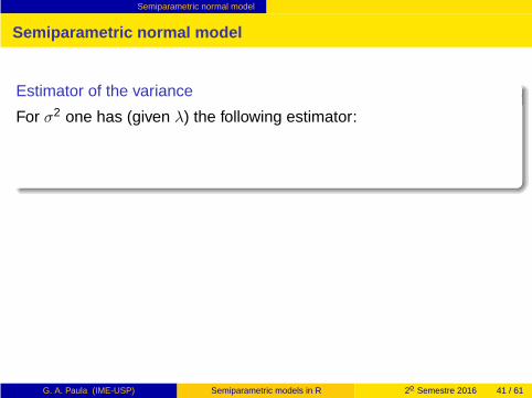
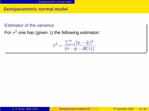
Estimator of the variance
For σ2 one has (given λ) the following estimator:
G. A. Paula (IME-USP) Semiparametric models in R 2o Semestre 2016 41 / 61
Semiparametric normal model
Semiparametric normal model
Estimator of the variance
For σ2 one has (given λ) the following estimator:
σ2 =
∑ni=1(yi − yi)
2
{n − p − df(λ)}.
G. A. Paula (IME-USP) Semiparametric models in R 2o Semestre 2016 41 / 61

Semiparametric normal model
Semiparametric normal model
Estimator of the variance
For σ2 one has (given λ) the following estimator:
σ2 =
∑ni=1(yi − yi)
2
{n − p − df(λ)}.
Choosing the smoothing parameter
Minimizing the generalized cross-validation score
GCV(λ) =n∑n
i=1(yi − yi)2
{n − df(λ)}2 ,
or minimizing (jointly) AIC(λ) and df(λ) for a grid of λ values.
G. A. Paula (IME-USP) Semiparametric models in R 2o Semestre 2016 41 / 61

Semiparametric normal model
Alternative penalization
P-splines
Eilers and Marx (1996) proposes the alternative penalization
G. A. Paula (IME-USP) Semiparametric models in R 2o Semestre 2016 42 / 61

Semiparametric normal model
Alternative penalization
P-splines
Eilers and Marx (1996) proposes the alternative penalization
SP(θ, λ) = (y − Xβ − Nτ )⊤(y − Xβ − Nτ ) + λ
q∑
j=d+1
[∆dτj ]2,
G. A. Paula (IME-USP) Semiparametric models in R 2o Semestre 2016 42 / 61

Semiparametric normal model
Alternative penalization
P-splines
Eilers and Marx (1996) proposes the alternative penalization
SP(θ, λ) = (y − Xβ − Nτ )⊤(y − Xβ − Nτ ) + λ
q∑
j=d+1
[∆dτj ]2,
where N is the de Boor’s basis and ∆dτj is the penalty difference termof order d .
In matrix notation
SP(θ, λ) = (y − Xβ − Nτ )⊤(y − Xβ − Nτ ) + λτ⊤D⊤
d Ddτ ,
where Dd is the penalty difference matrix of order d .
G. A. Paula (IME-USP) Semiparametric models in R 2o Semestre 2016 42 / 61

Semiparametric normal model
P-splines
Penalization examples
G. A. Paula (IME-USP) Semiparametric models in R 2o Semestre 2016 43 / 61

Semiparametric normal model
P-splines
Penalization examples
∆τj = τj − τj−1
D1 =
−1 1 0 00 −1 1 00 0 −1 1
.
G. A. Paula (IME-USP) Semiparametric models in R 2o Semestre 2016 43 / 61

Semiparametric normal model
P-splines
Penalization examples
∆τj = τj − τj−1
D1 =
−1 1 0 00 −1 1 00 0 −1 1
.
∆2τj = τj − 2τj−1 + τj−2
D2 =
1 −2 1 0 00 1 −2 1 00 0 1 −2 1
.
G. A. Paula (IME-USP) Semiparametric models in R 2o Semestre 2016 43 / 61

Semiparametric normal model
P-splines
Penalization examples
∆τj = τj − τj−1
D1 =
−1 1 0 00 −1 1 00 0 −1 1
.
∆2τj = τj − 2τj−1 + τj−2
D2 =
1 −2 1 0 00 1 −2 1 00 0 1 −2 1
.
∆3τj = τj − 3τj−1 + 3τj−2 − τj−3
D3 =
−1 3 −3 1 0 00 −1 3 −3 1 00 0 −1 3 −3 1
.
G. A. Paula (IME-USP) Semiparametric models in R 2o Semestre 2016 43 / 61
Packages in R
Outline
1 Examples
2 Defining f (x)
3 Additive normal model
4 Semiparametric normal model
5 Packages in R
6 Voltage drop data
7 Boston housing data
8 Bibliography
G. A. Paula (IME-USP) Semiparametric models in R 2o Semestre 2016 44 / 61

Packages in R
Packages in R
Packages in R
Some packages for fitting semi-parametric regression models availablefrom CRAN at http://CRAN.R-project.org:
G. A. Paula (IME-USP) Semiparametric models in R 2o Semestre 2016 45 / 61

Packages in R
Packages in R
Packages in R
Some packages for fitting semi-parametric regression models availablefrom CRAN at http://CRAN.R-project.org:
gamlss (Righy and Stasinopoulos, 2005)
G. A. Paula (IME-USP) Semiparametric models in R 2o Semestre 2016 45 / 61

Packages in R
Packages in R
Packages in R
Some packages for fitting semi-parametric regression models availablefrom CRAN at http://CRAN.R-project.org:
gamlss (Righy and Stasinopoulos, 2005)
mgcv (Wood, 2015)
G. A. Paula (IME-USP) Semiparametric models in R 2o Semestre 2016 45 / 61

Packages in R
Packages in R
Packages in R
Some packages for fitting semi-parametric regression models availablefrom CRAN at http://CRAN.R-project.org:
gamlss (Righy and Stasinopoulos, 2005)
mgcv (Wood, 2015)
ssym (Vanegas and Paula, 2015)
G. A. Paula (IME-USP) Semiparametric models in R 2o Semestre 2016 45 / 61

Voltage drop data
Outline
1 Examples
2 Defining f (x)
3 Additive normal model
4 Semiparametric normal model
5 Packages in R
6 Voltage drop data
7 Boston housing data
8 Bibliography
G. A. Paula (IME-USP) Semiparametric models in R 2o Semestre 2016 46 / 61

Voltage drop data
Scatter plot of voltage drop data
0 5 10 15 20
810
1214
Time
Volta
ge
G. A. Paula (IME-USP) Semiparametric models in R 2o Semestre 2016 47 / 61

Voltage drop data
Fitted model
Description
We will fit by the package ssym the following model:
Voltagei = α+ f (Timei) + ǫi ,
G. A. Paula (IME-USP) Semiparametric models in R 2o Semestre 2016 48 / 61

Voltage drop data
Fitted model
Description
We will fit by the package ssym the following model:
Voltagei = α+ f (Timei) + ǫi ,
where α is an intercept, f (·) is a continuous, smooth and
nonparametric function and ǫiiid∼ N(0, σ2) for i = 1, . . . , 41.
Suggestion: (n13 + 3) knots.
G. A. Paula (IME-USP) Semiparametric models in R 2o Semestre 2016 48 / 61

Voltage drop data
> require(ssym)> fit1.battery = ssym.l(voltage ~ ncs(time), data=battery,family="Normal")> summary(fit1.battery)
Family: NormalSample size: 41Quantile of the Weights0% 25% 50% 75% 100%1 1 1 1 1
************************** Median/Location submodel ********************************** Parametric component
Estimate Std.Err z-value Pr(>|z|)(Intercept) 10.904 0.0542 201.3309 < 2.2e-16 *********** Nonparametric component
Smooth.param Basis.dimen d.f. Statistic p-valuencs(time) 4.243 5.000 4.931 2709 <2e-16 ***
**** Deviance: 41
G. A. Paula (IME-USP) Semiparametric models in R 2o Semestre 2016 48 / 61

Voltage drop data
************************* Skewness/Dispersion submodel ******************************* Parametric component
Estimate Std.Err z-value Pr(>|z|)(Intercept) -2.3484 0.2209 -10.6329 < 2.2e-16 ***
**** Deviance: 42.2
*******************************************************************Overall goodness-of-fit statistic: 0.152165
-2*log-likelihood: 20.068AIC: 33.931BIC: 45.808
> np.graph(fit1.battery,which=1,xlab="Time", ylab="Voltage")> np.graph(fit1.battery,which=1,xlab="Time", ylab="Voltage",obs=TRUE)
G. A. Paula (IME-USP) Semiparametric models in R 2o Semestre 2016 49 / 61

Voltage drop data
Voltage 95% confidence band
0 5 10 15 20
−4−2
02
4
Voltage
Non
para
met
ric e
stim
ate
0 5 10 15 20
−4−2
02
4
Voltage
Non
para
met
ric e
stim
ate
G. A. Paula (IME-USP) Semiparametric models in R 2o Semestre 2016 49 / 61

Voltage drop data
Voltage 95% confidence band
0 5 10 15 20
−4−2
02
4
Voltage
Non
para
met
ric e
stim
ate
0 5 10 15 20
−4−2
02
4
0 5 10 15 20
−4−2
02
4
Voltage
Non
para
met
ric e
stim
ate
G. A. Paula (IME-USP) Semiparametric models in R 2o Semestre 2016 50 / 61

Boston housing data
Outline
1 Examples
2 Defining f (x)
3 Additive normal model
4 Semiparametric normal model
5 Packages in R
6 Voltage drop data
7 Boston housing data
8 Bibliography
G. A. Paula (IME-USP) Semiparametric models in R 2o Semestre 2016 51 / 61

Boston housing data
Plot of LMEDV versus NOX
0.4 0.5 0.6 0.7 0.8
2.0
2.5
3.0
3.5
4.0
NOX
LME
DV
G. A. Paula (IME-USP) Semiparametric models in R 2o Semestre 2016 52 / 61

Boston housing data
Plot of LMEDV versus NOX
0.4 0.5 0.6 0.7 0.8
2.0
2.5
3.0
3.5
4.0
NOX
LME
DV
G. A. Paula (IME-USP) Semiparametric models in R 2o Semestre 2016 53 / 61

Boston housing data
Plot of LMEDV versus LSTAT
10 20 30
2.0
2.5
3.0
3.5
4.0
LSTAT
LME
DV
G. A. Paula (IME-USP) Semiparametric models in R 2o Semestre 2016 54 / 61

Boston housing data
Plot of LMEDV versus LSTAT
10 20 30
2.0
2.5
3.0
3.5
4.0
LSTAT
LME
DV
G. A. Paula (IME-USP) Semiparametric models in R 2o Semestre 2016 55 / 61

Boston housing data
Possible model
Description
We may try to fit initially the following semi-parametric model:
LMEDVi = α+ βNOXi + f (LSTATi) + ǫi ,
G. A. Paula (IME-USP) Semiparametric models in R 2o Semestre 2016 56 / 61

Boston housing data
Possible model
Description
We may try to fit initially the following semi-parametric model:
LMEDVi = α+ βNOXi + f (LSTATi) + ǫi ,
where ǫiiid∼ N(0, σ2) for i = 1, . . . , 506, with f (·) being a continuous,
smooth and nonparametric function.
G. A. Paula (IME-USP) Semiparametric models in R 2o Semestre 2016 56 / 61

Boston housing data
> require(ssym)> require(MASS)> fit1.boston= ssym.l(log(medv) ~ nox + psp(lstat), data=Boston,family="Normal")
> summary(fit1.boston)
Family: NormalSample size: 506Quantile of the Weights0% 25% 50% 75% 100%1 1 1 1 1
************************** Median/Location submodel ********************************** Parametric component
Estimate Std.Err z-value Pr(>|z|)(Intercept) 3.1251 0.0650 48.0810 <2e-16 ***nox -0.1543 0.1106 -1.3954 0.1629
******** Nonparametric component
Smooth.param Basis.dimen d.f. Statistic p-valuepsp(lstat) 17.1 11.000 7.282 731.9 <2e-16 ***
G. A. Paula (IME-USP) Semiparametric models in R 2o Semestre 2016 56 / 61

Boston housing data
**** Deviance: 506
************************* Skewness/Dispersion submodel ******************************* Parametric component
Estimate Std.Err z-value Pr(>|z|)(Intercept) -2.9854 0.0629 -47.4859 < 2.2e-16 ***
**** Deviance: 762.68
*******************************************************************Overall goodness-of-fit statistic: 0.110987
-2*log-likelihood: -74.654AIC: -54.09BIC: -10.632
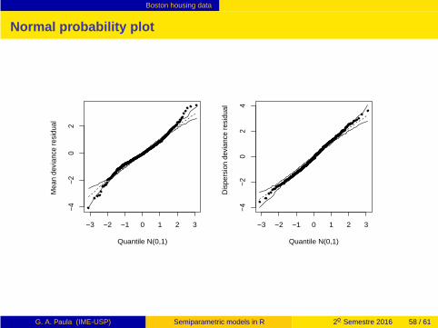
> np.graph(fit1.boston, which=1, xlab="Lstat",ylab="Estimate of f(Lstat)")> envelope(fit1.boston)
G. A. Paula (IME-USP) Semiparametric models in R 2o Semestre 2016 57 / 61

Boston housing data
f(Lstat) 95% confidence band
10 20 30
−1.0
−0.5
0.0
0.5
1.0
Lstat
Non
para
met
ric e
stim
ate
10 20 30
−1.0
−0.5
0.0
0.5
1.0
Lstat
Non
para
met
ric e
stim
ate
G. A. Paula (IME-USP) Semiparametric models in R 2o Semestre 2016 57 / 61
Boston housing data
Normal probability plot
−3 −2 −1 0 1 2 3
−4−2
02
Quantile N(0,1)
Mea
n de
vian
ce r
esid
ual
−3 −2 −1 0 1 2 3
−4−2
02
4Quantile N(0,1)
Dis
pers
ion
devi
ance
res
idua
l
G. A. Paula (IME-USP) Semiparametric models in R 2o Semestre 2016 58 / 61

Bibliography
Outline
1 Examples
2 Defining f (x)
3 Additive normal model
4 Semiparametric normal model
5 Packages in R
6 Voltage drop data
7 Boston housing data
8 Bibliography
G. A. Paula (IME-USP) Semiparametric models in R 2o Semestre 2016 59 / 61

Bibliography
References
References
G. A. Paula (IME-USP) Semiparametric models in R 2o Semestre 2016 60 / 61

Bibliography
References
References
Belsley DA, Kuh E and Welsch RE (1980). RegressionDiagnostics. Identifying Influential Data and Sources ofCollinearity. Wiley, New York.
G. A. Paula (IME-USP) Semiparametric models in R 2o Semestre 2016 60 / 61

Bibliography
References
References
Belsley DA, Kuh E and Welsch RE (1980). RegressionDiagnostics. Identifying Influential Data and Sources ofCollinearity. Wiley, New York.
De Boor C (1978). A Practical Guide to Splines. AppliedMathematical Sciences. Springer-Verlag, New York.
Eilers PHC and Marx BD (1996). Flexible smoothing withB-splines and penalties. Statistical Science, 11, 89-121.
Green PJ and Silverman BW (1994). Nonparametric Regressionand Generalized Linear Models. Chapman and Hall, London.
Hastie TJ and Tibshirani RJ (1990). Generalized Additive Models.Chapman and Hall, London.
G. A. Paula (IME-USP) Semiparametric models in R 2o Semestre 2016 60 / 61

Bibliography
References
References
G. A. Paula (IME-USP) Semiparametric models in R 2o Semestre 2016 61 / 61

Bibliography
References
References
Montgomery DC, Peck EA and Vining GG (2001). Introduction toLinear Regression Analysis, 3rd Edition. Wiley, New York.
G. A. Paula (IME-USP) Semiparametric models in R 2o Semestre 2016 61 / 61

Bibliography
References
References
Montgomery DC, Peck EA and Vining GG (2001). Introduction toLinear Regression Analysis, 3rd Edition. Wiley, New York.
Paula GA (2013). On diagnostics in double generalized linearmodels. Computational Statistics & Data Analysis, 68, 44-51.
Righy, R. A. e Stasinopoulos, D. M. (2005). Generalized additivemodels for location, scale and shape (with discussion). AppliedStatistics 54, 507-554.
Vanegas LH and Paula GA (2015). ssym: Fitting Semi-parametricLog-symmetric Regression Models. R package version 1.5.3.http://CRAN.R-project.org/package=ssym.
Wood SN (2015). mgcv: Mixed GAM Computation Vehicle withGCV/AIC;REML. Smoothness Estimation R package version1.8-7. http://CRAN.R-project.org/package=mgcv.
G. A. Paula (IME-USP) Semiparametric models in R 2o Semestre 2016 61 / 61