gis: fast indexing and querying of graph structuresr.web.umkc.edu/raopr/tr-db-2009-01.pdf · we...
TRANSCRIPT

GiS: Fast Indexing and Querying of Graph Structures ∗
Dipali Pal Praveen R. Rao Vasil Slavov
{[email protected],[email protected],[email protected]}
Technical Report UMKC-TR-DB-2009-01
Abstract
We propose a new way of indexing a large database of graphs and processing exact subgraph matching
(or subgraph isomorphism) and approximate (full) graph matching queries. Rather that decomposing a
graph into smaller units (e.g., paths, trees, graphs) for indexing purposes, we represent each graph in
the database by its graph signature, which is essentially a multiset, and each signature is then indexed.
During query processing, a query graph is also mapped into its signature. We show that exact subgraph
matching and approximate (full) graph matching queries can be processed by performing operations
such as intersection and union over the data and query graph signatures. We call this holistic query
processing where a query is processed as a whole without decomposing into smaller units. To improve
the precision of exact subgraph matching, we propose a new method based on the concept of line graphs.
We study its benefits and tradeoffs for a variety of datasets. To speed up query processing, we develop a
disk-based index on graph signatures and propose a bulk-loading scheme for fast indexing. We study the
relationship between graph edit distance and the properties of graph signatures and develop a method for
approximate (full) graph matching. Through extensive evaluation on real and synthetic graph datasets,
we demonstrate that GiS’s holistic query processing approach provides a scalable and efficient disk-based
solution for indexing and querying graphs.
Nov 2009
(Updated Nov 2012)
Department of Computer Science and Electrical Engineering
University of Missouri-Kansas City
Kansas City, MO 64110
∗The authors assume all responsibility for the contents of the paper.
0

1 Introduction
Graphs are widely used to model data in a variety of domains such as biology, chemistry, computer vision,and the World Wide Web. As an example, in biology, protein interaction networks and phylogenies can bemodeled as graphs. In chemistry, chemical compound structures can be conveniently represented by graphstructures. Graphs are also useful in pattern recognition and computer vision, for example, to representhierarchical image features. On the World Wide Web, social networks naturally fit a graph data model.
Pattern matching over graphs is an important task in a variety of applications and falls under twocategories, namely, subgraph matching and entire graph matching. Further, each category can be classifiedinto exact matching and approximate (or in-exact) matching. Exact subgraph matching (or isomorphism) [34,20] has been a problem of interest for several decades and has been widely used in areas such as chemicalinformatics, circuit design and verification, scene analysis in computer vision, and so forth. One exampleis the task of substructure matching in chemical databases. By posing a query based on exact subgraphmatching, we can identify those molecules in a database that contain a particular functional group (e.g., aphenyl group C6H5) [11]. Another application of exact subgraph matching is for finding structural motifs in3D protein structures using protein contact maps [17], which can be represented as labeled graphs.
Approximate graph matching [36] is useful in applications where graphs similar to a query graph are de-sired. Such a matching is useful for tasks such as similarity searching of chemical compounds [37], comparingphylogenies and biopathway graphs, and so forth.
Subgraph isomorphism is an NP-complete problem [9], for which backtracking techniques [34, 14] weredeveloped in the past. Unfortunately, these techniques become intractable in the worst case. In practicalapplications a large number of graphs exist in the database, and it is infeasible to test for subgraph isomor-phism pairwise between a query graph and every data graph. A common approach adopted by most priortechniques is to first filter and identify candidate matches, and then verify these candidates to retain onlythe true matches. The key challenge in the filtering stage is to construct an index over graphs, so that a largenumber of graphs that do not contain a match for a query can be pruned away quickly, thereby reducing thenumber of actual pairwise tests needed in the verification stage.
Many of the previous approaches for exact subgraph matching queries are main-memory based i.e., theyload the index into memory before processing graph queries (e.g., gIndex [40], Grafil [41], Tree+∆ [47],GDIndex [38], QuickSI [30], GCoding [48]). A recent technique called FG-index [6, 7] maintains part of theindex in memory and the rest on disk. SAGA [31] and TALE [32] are disk-based techniques for approximatesubgraph matching queries.
Previous approaches commonly leverage frequent pattern mining to extract features from graphs (e.g.,trees, subgraphs) for indexing (e.g., gIndex [40], Grafil [41], Tree+∆ [47], QuickSI [30], FG-index [6, 7]).GraphGrep [10] and SING [22] use paths in graphs as features but do not use frequent pattern mining.C-tree [15] and GCoding [48] are two other techniques that do not rely on mining to construct indexes ongraphs.
Approximate graph matching requires the computation of graph edit distance between graphs. Graph editdistance provides a measure of dissimilarity between two graphs. However, computing graph edit distancebetween two graphs is computationally expensive and the cost is exponential in the number of vertices in thegraphs [28]. Therefore, to process an approximate graph matching query, it would be inefficient to computethe graph edit distance between a query and every graph in the database. A filter and verification approachseems to be a viable alternative.
In this work, we aim to build disk based indexes for fast filtering of exact subgraph and approximategraph matching queries. This will allow us to process large datasets wherein the graph indexes cannot fitin main memory. We aim to avoid the use of mining for extracting frequent patterns as this preprocessingstep can become very expensive for large, dense graphs. Finally, holistic XML pattern matching approaches(e.g., TwigStack [3]) are regarded to be superior for querying XML documents than those that decomposea tree pattern query into smaller units and process them separately. In a similar vein, we aim to developa holistic graph pattern matching approach, without decomposing a graph (data or query) into its featuresduring indexing and query processing.
The nature of data graphs supported by GiS is illustrated in Figure 1. In Figure 1(a), an undirectedgraph (without edge labels) is used to represent the 3D structure of proteins using contact map graphs [8].In Figure 1(b), an undirected graph (with edge labels) is used to model a guanine molecule.
1

NH2
O
NH
NN
N
H
O
C
CH
N
C
N
CN
C
N
HN
H
H
d
d
ds
s
s
ss
ss
s
s
s
s
ds
(a) Protein contact map graphs (b) Guanine molecule
Figure 1: Examples
To achieve our aforementioned aims, we propose a system called GiS. We assume that the databaseD has a large number of labeled, undirected graphs. The nature of real-world data graphs studied in thispaper include contact map graphs to represent 3D structure of proteins [8] and graphs representing chemicalmolecules. We also consider larger graphs such as protein-protein interaction networks. We address twotypes of queries over D.
Exact subgraph matching: Given a query graph Q, an exact subgraph matching query findsall graphs in D that contain a subgraph that is isomorphic to Q. (This query is also referred toas a subgraph containment query in prior work.)
Approximate (full) graph matching: Given a query graph Q and a distance threshold d, anapproximate graph matching query finds all graphs in D whose edit distance with Q is at mostd.
The key contributions of this paper are summarized below.
• We propose a new way of representing a graph holistically (i.e., as a whole) by its signature, therebyavoiding its decomposition into smaller units that are separately indexed. A graph signature is essen-tially a multiset that captures the vertex and edge characteristics of a graph.
• To systematically expose more structural properties of a graph that can be captured by a graphsignature, and therefore, improve the precision of exact subgraph matching, we propose a new methodbased on the concept of line graphs. Line graph computation can be applied successively to a graphand provides a way to tune the extent of structural information captured by signatures. We study thebenefits and tradeoffs of our method.
• We propose an approach for approximate graph matching using signatures on the original graphs.(Line graphs are not used for approximate graph matching.) We study the relationship between graphedit distance and the properties of graph signatures and propose a method for processing approximategraph matching queries.
• We show that both exact subgraph matching and approximate graph matching query can be processedby first computing the signature of a query and then by applying multiset operations on the dataand query signatures. Unlike GiS, many existing methods decompose a query into features and thenprocess individual features and combine the results.
2

• To speed up query processing, we develop a disk-based indexing strategy for graph signatures, i.e.,multisets. We propose a bulk-loading approach for efficient indexing.
• We demonstrate through extensive performance evaluation on real and synthetic graph datasets thatGiS’s holistic query processing approach provides an efficient disk-based solution for the filtering phaseof exact subgraph matching and approximate graph matching.
The rest of the paper is organized as follows: Section 2 provides preliminaries in graph theory andmultisets; Section 3 describes related work; Section 4 provides the overall architecture of GiS; Section 5presents graph signatures and line graphs; Section 6 describes how signatures can be used for exact subgraphmatching; Section 7 describes approximate graph matching using signatures; Section 8 describes our indexingstrategy and query processing algorithms; Section 9 describes the performance evaluation; and Section 10describes our conclusions and future work.
This work was presented as a demonstration at a conference [24].
2 Preliminaries
We state the basic terminologies from graph theory literature. A graph G consists of a non-empty finitevertex set V (G) called vertices, and a finite set E(G) of unordered pairs of vertices called edges. We denotesuch a graph by G(V,E) or G = (V,E). A simple graph, which we consider in this paper, does not containmulti-edges or self-loops. We assume undirected graphs, where there is no direction assigned to an edge.Edges and vertices may be labeled. We assume that each vertex of a graph is assigned a unique integer idfrom 1 to n, where n denotes the number of vertices. We use vi to denote the id of a vertex. Let l(vi) denotethe vertex label of vi drawn from some domain D. Two vertices are adjacent if there is an edge joining them.An edge is said to be incident on the vertices that are its end points. We will frequently use (vi, vj) to denotean edge between vertex vi and vertex vj . Two edges are adjacent if they share a common vertex.
A graph G1 is isomorphic to G2, if there exists a bijective mapping f : V (G1) → V (G2) between thevertex sets in G1 and G2, and two vertices u1 and v1 are adjacent in G1, if and only if, their correspondingvertices u2 and v2 are adjacent in G2. A subgraph Gi(Vi, Ei) of a graph G has a vertex set Vi ⊆ V andEi ⊆ E. Subgraph isomorphism is a decision problem to test if a graph has a subgraph that is isomorphicto a given graph. For labeled graphs, we impose an additional condition that the labels of correspondingvertices in the bijective mapping should also be identical for graph and subgraph isomorphism.
Edit distance between two graphs denotes the minimum cost of transforming one graph to another byapplying a sequence of edit operations (e.g., insertion, deletion, and relabel of vertices and edges). Inapproximate graph matching, we find those graphs that are within a user-specified edit distance from aquery graph.
Example 1 Figure 2 shows three data graphs G1, G2, and G3, and one query graph Q. The domain ofvertex labels D = {A,B,C}. In G3, there exists a subgraph that is isomorphic to Q as shown by dottedarrows. Only G2 has an edit distance of one with Q (assuming unit costs for each edit operation). Onevertex relabel is needed to transform G2 to Q. G1 and G3, however, have an edit distance greater than onewith Q.
G1 G2 Q
BA
C
A
BB
A CC B
B
B
B
A
C
C
G3
Figure 2: Examples
3
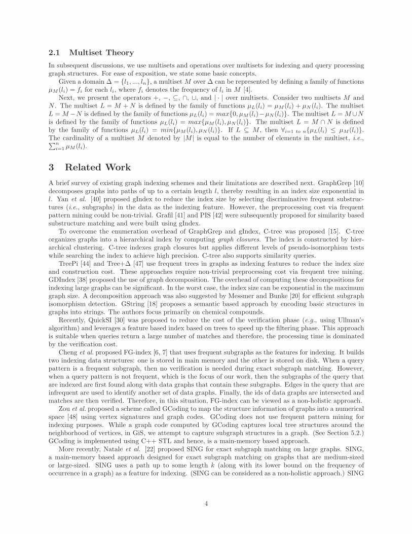
2.1 Multiset Theory
In subsequent discussions, we use multisets and operations over multisets for indexing and query processinggraph structures. For ease of exposition, we state some basic concepts.
Given a domain ∆ = {l1, ..., ln}, a multiset M over ∆ can be represented by defining a family of functionsµM (li) = fi for each li, where fi denotes the frequency of li in M [4].
Next, we present the operators +, −, ⊆, ∩, ∪, and | · | over multisets. Consider two multisets M andN . The multiset L = M +N is defined by the family of functions µL(li) = µM (li) + µN (li). The multisetL = M −N is defined by the family of functions µL(li) = max{0, µM (li)−µN (li)}. The multiset L = M ∪Nis defined by the family of functions µL(li) = max{µM (li), µN (li)}. The multiset L = M ∩ N is definedby the family of functions µL(li) = min{µM (li), µN (li)}. If L ⊆ M , then ∀i=1 to n{µL(li) ≤ µM (li)}.The cardinality of a multiset M denoted by |M | is equal to the number of elements in the multiset, i.e.,∑n
i=1 µM (li).
3 Related Work
A brief survey of existing graph indexing schemes and their limitations are described next. GraphGrep [10]decomposes graphs into paths of up to a certain length l, thereby resulting in an index size exponential inl. Yan et al. [40] proposed gIndex to reduce the index size by selecting discriminative frequent substruc-tures (i.e., subgraphs) in the data as the indexing feature. However, the preprocessing cost via frequentpattern mining could be non-trivial. Grafil [41] and PIS [42] were subsequently proposed for similarity basedsubstructure matching and were built using gIndex.
To overcome the enumeration overhead of GraphGrep and gIndex, C-tree was proposed [15]. C-treeorganizes graphs into a hierarchical index by computing graph closures. The index is constructed by hier-archical clustering. C-tree indexes graph closures but applies different levels of pseudo-isomorphism testswhile searching the index to achieve high precision. C-tree also supports similarity queries.
TreePi [44] and Tree+∆ [47] use frequent trees in graphs as indexing features to reduce the index sizeand construction cost. These approaches require non-trivial preprocessing cost via frequent tree mining.GDIndex [38] proposed the use of graph decomposition. The overhead of computing these decompositions forindexing large graphs can be significant. In the worst case, the index size can be exponential in the maximumgraph size. A decomposition approach was also suggested by Messmer and Bunke [20] for efficient subgraphisomorphism detection. GString [18] proposes a semantic based approach by encoding basic structures ingraphs into strings. The authors focus primarily on chemical compounds.
Recently, QuickSI [30] was proposed to reduce the cost of the verification phase (e.g., using Ullman’salgorithm) and leverages a feature based index based on trees to speed up the filtering phase. This approachis suitable when queries return a large number of matches and therefore, the processing time is dominatedby the verification cost.
Cheng et al. proposed FG-index [6, 7] that uses frequent subgraphs as the features for indexing. It buildstwo indexing data structures: one is stored in main memory and the other is stored on disk. When a querypattern is a frequent subgraph, then no verification is needed during exact subgraph matching. However,when a query pattern is not frequent, which is the focus of our work, then the subgraphs of the query thatare indexed are first found along with data graphs that contain these subgraphs. Edges in the query that areinfrequent are used to identify another set of data graphs. Finally, the ids of data graphs are intersected andmatches are then verified. Therefore, in this situation, FG-index can be viewed as a non-holistic approach.
Zou et al. proposed a scheme called GCoding to map the structure information of graphs into a numericalspace [48] using vertex signatures and graph codes. GCoding does not use frequent pattern mining forindexing purposes. While a graph code computed by GCoding captures local tree structures around theneighborhood of vertices, in GiS, we attempt to capture subgraph structures in a graph. (See Section 5.2.)GCoding is implemented using C++ STL and hence, is a main-memory based approach.
More recently, Natale et al. [22] proposed SING for exact subgraph matching on large graphs. SING,a main-memory based approach designed for exact subgraph matching on graphs that are medium-sizedor large-sized. SING uses a path up to some length k (along with its lower bound on the frequency ofoccurrence in a graph) as a feature for indexing. (SING can be considered as a non-holistic approach.) SING
4

Figure 3: Architecture of GiS
also maintains the position of a feature in a graph to speed up the filtering phase and the verification phase.Unlike GiS, SING supports the finding of all occurrences of an exact subgraph match in the graph database.
Many approaches have been developed for approximate subgraph matching (e.g., SAGA [31], TALE [32],PIS [42], Grafil [41],GADDI [45], GrafD-index [29], SAPPER [46]). SAGA [31] and TALE [32] are diskbased approaches for approximate subgraph matching. SAGA is designed for small query graphs and TALEis designed for large query graphs with hundreds of nodes. SAGA is suited for biological data and breaks agraph into fragments of a user-specified size and uses fragments as the indexing units. In TALE, the indexingunit is the neighborhood of each graph node. The neighborhood information captures the local structurearound a graph node, and the index size grows linearly with the database size. TALE can be regarded as anon-holistic approach. SAPPER is another technique for approximate subgraph matching on large graphs.Unlike, TALE that is faster but may miss approximate matches, SAPPER returns all matches. GiS is notdesigned for approximate subgraph matching.
Recently, Cheng et al. [5] proposed a new approach for processing supergraph queries, wherein thedatabase graphs that are contained by the query graph are output. GiS does not support supergraphqueries. Han et al. [13] developed a framework called iGraph by reimplementing previous techniques suchas gIndex, FG-index, Tree+∆, C-tree, and GCoding to enable their comparison based on the I/O cost. Thisframework was developed on MS Windows platform.
The concept of a line graph has been studied in the context of biological networks. Periera et al. [25]used the line graph of a protein interaction network to improve graph clustering. Ucar et al. [33] used theline graph for preprocessing to eliminate redundant false positives from protein-protein interactions beforeperforming clustering. Nacher et al. [21] studied the effect of line graph computation on scale-free networks.Bayir et al. [1] computed the line graph of protein interaction network to remove edges in the graph beforecomputing topological measures.
In this paper, we employ the concept of line graphs in the context of processing exact subgraph matchingqueries. We analyze the properties of line graphs when applied multiple times on graphs (with and withoutedge labels) and empirically show that line graphs enable high precision of exact subgraph matching.
4 Architecture of GiS
We introduce the overall architecture of GiS before delving into the details of its design in Sections 5, 6, 7,and 8. The key components of GiS include the Signature Generator, Indexing Engine, Query Engine, andStorage Engine as shown in Figure 3. The Signature Generator constructs a signature of a graph and cangenerate different quality signatures using the idea of line graphs. A graph signature is essentially a multisetrepresentation of a graph that captures the vertex and edge characteristics of the graph and enables holistic
5
processing of graph queries.To index a graph, the Indexing Engine obtains the signature of a graph from the Signature Generator
and then indexes the signature in a disk-resident hierarchical index. The index, which we refer to as graphsignature index, speeds up the filtering phase during query processing. The leaf nodes of the graph signatureindex contain the graph signatures and the ids of the graphs. The Storage Engine maintains the indexes andthe data graphs on disk. A user can pose either an exact subgraph matching query or an approximate (full)graph matching query.
The Query Engine obtains the signature of a query graph from the Signature Generator and then usesit as a key to search through the signature index. Candidates graph ids are obtained during the filteringphase. Finally, the verification step is carried out on the candidate graphs to obtain the true matches for thequery. Note that the way the signature index is searched during the filtering phase depends on the natureof the query. For example, subset operation between multisets (or signatures) is utilized for exact subgraphmatching; multiset difference operation is utilized during approximate graph matching.
5 Graph Signatures
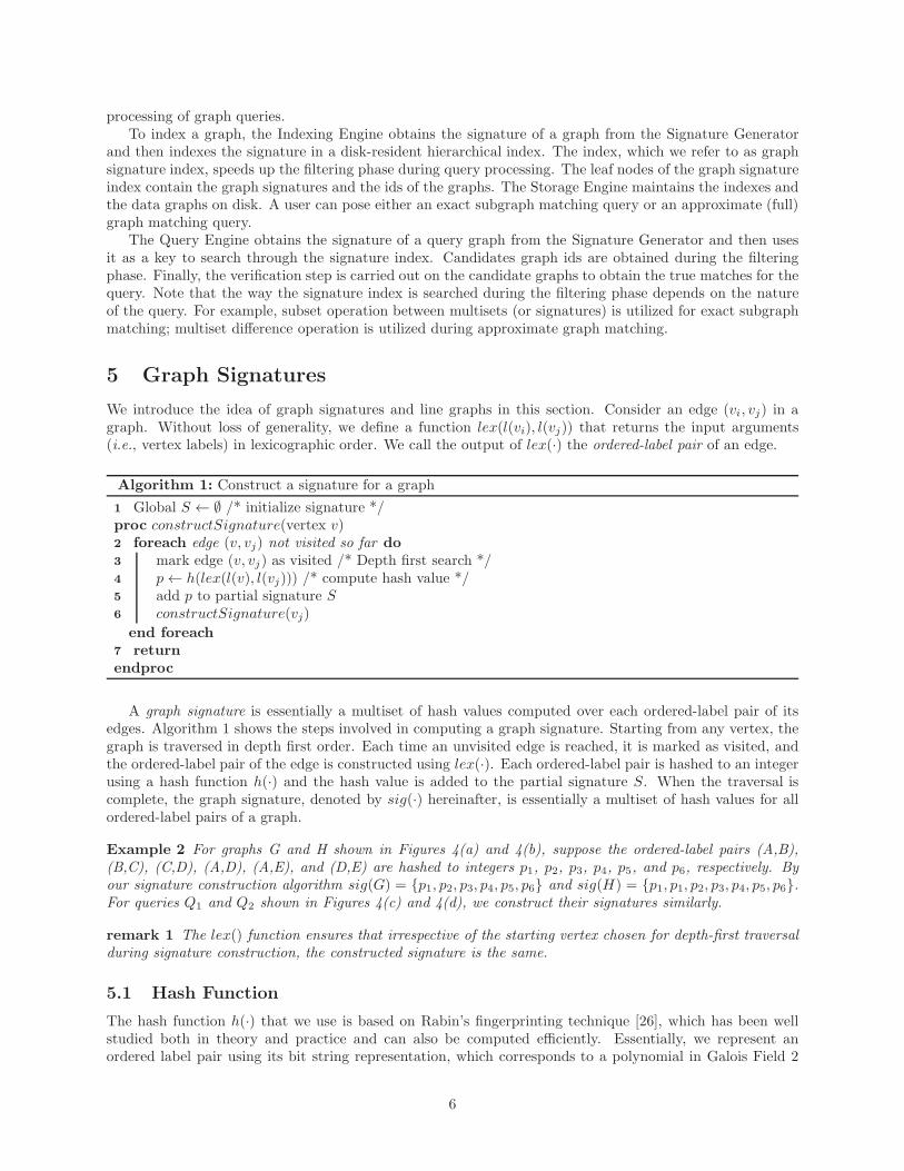
We introduce the idea of graph signatures and line graphs in this section. Consider an edge (vi, vj) in agraph. Without loss of generality, we define a function lex(l(vi), l(vj)) that returns the input arguments(i.e., vertex labels) in lexicographic order. We call the output of lex(·) the ordered-label pair of an edge.
Algorithm 1: Construct a signature for a graph
1 Global S ← ∅ /* initialize signature */proc constructSignature(vertex v)2 foreach edge (v, vj) not visited so far do3 mark edge (v, vj) as visited /* Depth first search */4 p← h(lex(l(v), l(vj))) /* compute hash value */5 add p to partial signature S
6 constructSignature(vj)
end foreach7 returnendproc
A graph signature is essentially a multiset of hash values computed over each ordered-label pair of itsedges. Algorithm 1 shows the steps involved in computing a graph signature. Starting from any vertex, thegraph is traversed in depth first order. Each time an unvisited edge is reached, it is marked as visited, andthe ordered-label pair of the edge is constructed using lex(·). Each ordered-label pair is hashed to an integerusing a hash function h(·) and the hash value is added to the partial signature S. When the traversal iscomplete, the graph signature, denoted by sig(·) hereinafter, is essentially a multiset of hash values for allordered-label pairs of a graph.
Example 2 For graphs G and H shown in Figures 4(a) and 4(b), suppose the ordered-label pairs (A,B),(B,C), (C,D), (A,D), (A,E), and (D,E) are hashed to integers p1, p2, p3, p4, p5, and p6, respectively. Byour signature construction algorithm sig(G) = {p1, p2, p3, p4, p5, p6} and sig(H) = {p1, p1, p2, p3, p4, p5, p6}.For queries Q1 and Q2 shown in Figures 4(c) and 4(d), we construct their signatures similarly.
remark 1 The lex() function ensures that irrespective of the starting vertex chosen for depth-first traversalduring signature construction, the constructed signature is the same.
5.1 Hash Function
The hash function h(·) that we use is based on Rabin’s fingerprinting technique [26], which has been wellstudied both in theory and practice and can also be computed efficiently. Essentially, we represent anordered label pair using its bit string representation, which corresponds to a polynomial in Galois Field 2
6

p2p3
p4
p5
p6
1p
B
A
C
D
E p1
p2
p3
p6
p5
p4
A
B A E
DC
p1 B
p2
p1
A
B
C
p1
p7
A
B
C
(a) Graph G (b) Graph H (c) Q1 (d) Q2
Figure 4: Data and query graphs with hash values assigned to each ordered-labeled pair.
with coefficients 0 or 1. Let us denote this polynomial by p. We define h(·) = p mod r, where r is anirreducible polynomial in Galois Field 2 picked at random. This hash function has low degree of collision.Suppose k bit fingerprints are computed using an irreducible polynomial of degree k − 1, then given two
ordered label pairs x and y, s.t. x 6= y, P (h(x) = h(y)) ≤ max(|x|,|y|)2k−1 , where | · | denotes the number of
bits [2].In our experiments, r was an irreducible polynomial of degree 31 and we generated 32 bit hash values.
Suppose each ordered labeled pair requires at most 1024 bits, then the probability of collision is less than2−21. We required less than 1024 bits for each ordered label pair in our experiments.
5.2 Line Graphs: A Method to Tune Graph Signatures
The above scheme for signature construction solely considers adjacent vertices and their labels. It ignoresother structural properties of a graphs such as adjacency between the edges in the graph, which can affectthe precision of exact subgraph matching. We propose a new method that allows GiS to tune the amount ofstructural information captured by graph signatures based on the concept of line graphs (a.k.a. interchangegraphs) [39].
Definition 1 A line graph of a graph G = (V,E), denoted by L(G) = (VL, EL), is a graph whose vertex setVL contains one vertex for every edge in G. The edge set EL is constructed as follows: two vertices in L(G)are adjacent, if and only if, their corresponding edges in G are adjacent i.e., share a vertex.
Although the standard definition of a line graph does not specify how the vertex labels of a line graphshould be represented, we follow a precise way, because this affects the graph signatures that will be con-structed. For an edge (vi, vj) in G, we label the corresponding vertex in L(G) by lex(l(vi), l(vj)).
Algorithm 2 outlines the steps involved in constructing L(G) from G. It has two phases: In the firstphase, the vertex set of L(G) is created by traversing G in depth-first order (Lines 3-10). In the secondphase, we examine the adjacency between edges in G and create the edge set of L(G) (Lines 11-20).
The signature of L(G) is constructed using the signature construction algorithm described earlier (Algo-rithm 1). The ordered-label pair of each edge in the line graph is also computed using the function lex(·) andis then hashed to an integer during signature construction. Note that the signature of a line graph containsthe hash values of the ordered-label pairs in it.
Example 3 L(G) and L(H) in Figures 5(a) and 5(b) denote the line graphs of G and H in Figures 4(a)and 4(b), respectively. The ordered-label pairs of L(G) and L(H) are hashed to integers r0, ..., r9. For exam-ple, the ordered-label pair ((A,B),(B,C)) is hashed to r1. The signatures sig(L(G)) = {r1, r2, r3, r4, r5, r6,r7, r8, r9} and sig(L(H))= {r0, r1, r2, r3, r4, r7, r8, r9}. For query Q3 in Figure 5(c), its line graph L(Q3) is shown and its signaturesig(L(Q3)) = {r1, r2, r6, r9}.
A line graph of a graph provides a systematic way to expose more structural properties of a graph thatcan be captured during signature construction: L(G) explicitly provides the information about the adjacencyof edges in G. (Line graph computation can be applied again on L(G). It is similar to a composable function.This property of line graphs is discussed in Section 5.3.) We assert that line graphs provide a way to tunethe quality of graph signatures, while still enabling holistic processing of queries.
7

r5
r2r8
r4
r7
3r
r1
r6
r9
A,B
A,D
B,C
C,DD,E
A,Er1
r2
3r
r8
r7
r4
r9
A,B
A,D
B,C
C,DD,E
A,E
A,Br0
p1 p4
p3p2Q3
r6r1
r2 r9
L(Q3)
C
B
A
D
A,B
B,C A,D
C,D
(a) L(G) (b) L(H) (c) Q3 and L(Q3)
Figure 5: Data and query line graphs.
Thus, rather than indexing the signatures of the data graphs, we can index the signatures of their linegraphs. (The benefit achieved by using line graphs during exact subgraph matching will be illustrated inSection 6 through an example.) Although a line graph improves the quality of signatures, it increases thelength of signatures in most cases. Given a graph G = (V,E) and its L(G) = (VL, EL), |VL| = |E| and
|EL| =∑|V |
i=1
(
deg(vi)2
)
, where deg(vi) is the degree of a vertex vi in G. The time complexity of constructinga line graph is O(|VL|+ |EL|).
Note that there are two exceptions as shown by Rooij et al. [35]. If a graph is a path graph (i.e., containsonly one path) with path length n, then its line graph is a path graph with path length n− 1. In this case,the size of the signature will decrease as fewer edges will be considered. If a graph is a cycle graph, then itsline graph is also a cycle graph. In this case, the size of the signature remains the same.
5.3 Successively Applying Line Graph Computation for Exact Subgraph Match-ing
A graph signature can be made more precise by successively applying the line graph computation n times onthe input graph. (Line graph computation is similar to a composable function.) As a result, the structuralproperties captured by the signature are enhanced. We denote the successive application of line graphcomputation by Ln(G), where G is the input graph. For example, L3(G) is equivalent to L(L(L(G))). Ifn = 0, L0(G) = G. We refer to each Li(G) as a line graph in our discussions. Except for path graphs, allother input graphs will yield a graph for Ln(·) as n→∞.
Example 4 Figure 6(a) shows the successive application of line graph computation, where the number ofedges grows. Figure 6(b) shows the successive application of line graph computation on a cycle graph.
From a line graph Ln(G), we apply Algorithm 1 and construct its signature by hashing the ordered-labelpairs in it, as we did for the original graph G. Thus, we do not need to store the vertex labels of a linegraphs. The size of the signature of a line graph grows with the number of edges in the line graph and doesnot depend on the size of the vertex labels. (A more detailed discussion is provided in Section 6.3.)
Example 5 Consider L(L(G)) in Figure 6(b). The ordered-label pairs (output by the lex(·) function) are‘((A,B),(B,C)), ((B,C),(B,E))’, ‘((A,B),(B,C)), ((B,C),(C,D))’, ‘((A,B),(B,C)), ((A,B),(B,E))’, ‘((A,B),(B,E)),((B,C),(B,E))’, ‘((A,B),(B,E)), ((B,E),(D,E))’, ‘((B,C),(B,E)), ((B,C),(C,D))’, ‘((B,C),(B,E)), ((B,E),(D,E))’,‘((B,C),(C,D)), ((C,D),(D,E))’, and ‘((B,E),(D,E)), ((C,D),(D,E))’. The signature of L(L(G)) will contain9 hash values after hashing each of the above ordered-label pairs.
Now, we can index sig(Ln(G)) instead of sig(G). We show through our experimental evaluation inSection 9, that line graphs improves the precision of exact subgraph matching queries. For instance, with areal dataset, the average precision improved from 0.58 to 0.997 when sig(L2(G)) was used instead of sig(G).The intuition for the improvement is as follows: With successive application of line graph computation,
8
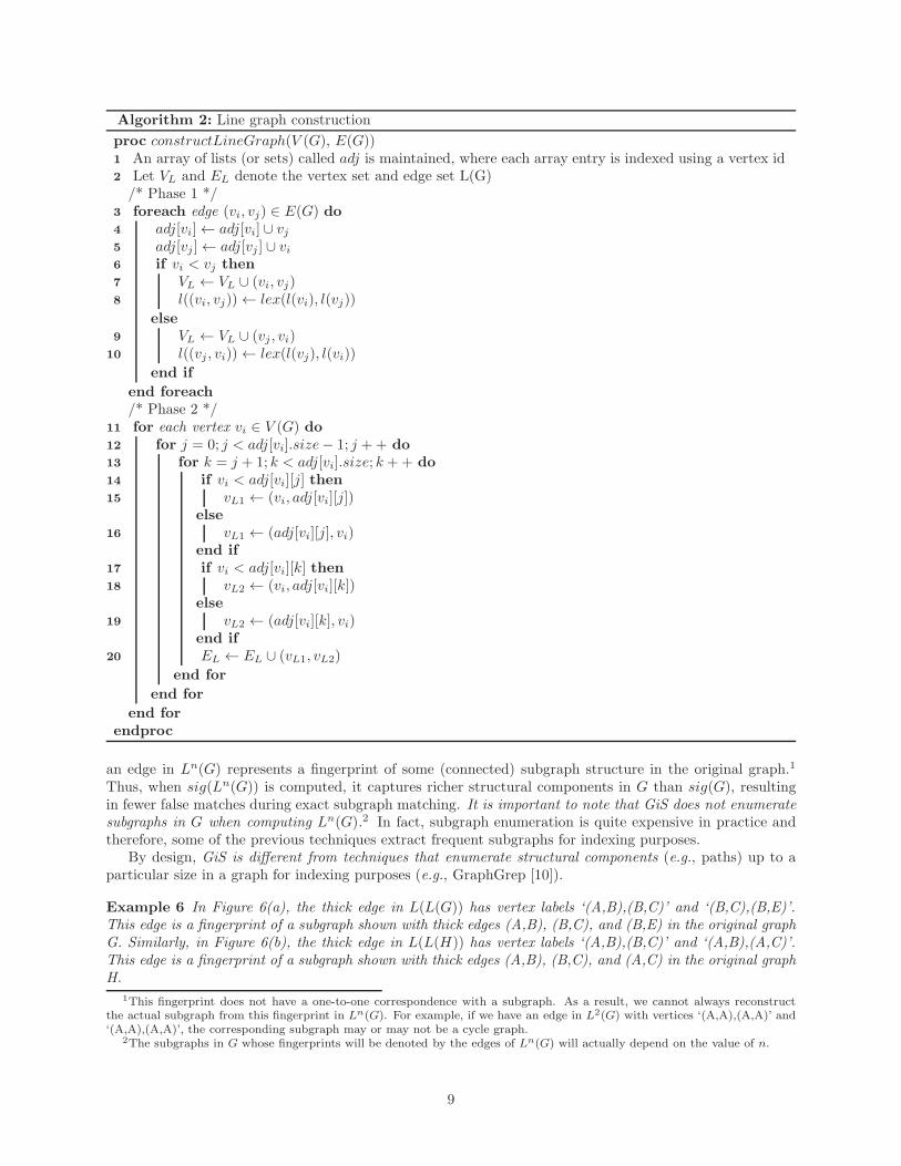
Algorithm 2: Line graph construction
proc constructLineGraph(V (G), E(G))1 An array of lists (or sets) called adj is maintained, where each array entry is indexed using a vertex id2 Let VL and EL denote the vertex set and edge set L(G)/* Phase 1 */
3 foreach edge (vi, vj) ∈ E(G) do4 adj[vi]← adj[vi] ∪ vj5 adj[vj ]← adj[vj ] ∪ vi6 if vi < vj then7 VL ← VL ∪ (vi, vj)8 l((vi, vj))← lex(l(vi), l(vj))
else9 VL ← VL ∪ (vj , vi)
10 l((vj , vi))← lex(l(vj), l(vi))
end if
end foreach/* Phase 2 */
11 for each vertex vi ∈ V (G) do12 for j = 0; j < adj[vi].size− 1; j ++ do13 for k = j + 1; k < adj[vi].size; k ++ do14 if vi < adj[vi][j] then15 vL1 ← (vi, adj[vi][j])
else16 vL1 ← (adj[vi][j], vi)
end if17 if vi < adj[vi][k] then18 vL2 ← (vi, adj[vi][k])
else19 vL2 ← (adj[vi][k], vi)
end if20 EL ← EL ∪ (vL1, vL2)
end for
end for
end forendproc
an edge in Ln(G) represents a fingerprint of some (connected) subgraph structure in the original graph.1
Thus, when sig(Ln(G)) is computed, it captures richer structural components in G than sig(G), resultingin fewer false matches during exact subgraph matching. It is important to note that GiS does not enumeratesubgraphs in G when computing Ln(G).2 In fact, subgraph enumeration is quite expensive in practice andtherefore, some of the previous techniques extract frequent subgraphs for indexing purposes.
By design, GiS is different from techniques that enumerate structural components (e.g., paths) up to aparticular size in a graph for indexing purposes (e.g., GraphGrep [10]).
Example 6 In Figure 6(a), the thick edge in L(L(G)) has vertex labels ‘(A,B),(B,C)’ and ‘(B,C),(B,E)’.This edge is a fingerprint of a subgraph shown with thick edges (A,B), (B,C), and (B,E) in the original graphG. Similarly, in Figure 6(b), the thick edge in L(L(H)) has vertex labels ‘(A,B),(B,C)’ and ‘(A,B),(A,C)’.This edge is a fingerprint of a subgraph shown with thick edges (A,B), (B,C), and (A,C) in the original graphH.
1This fingerprint does not have a one-to-one correspondence with a subgraph. As a result, we cannot always reconstructthe actual subgraph from this fingerprint in Ln(G). For example, if we have an edge in L2(G) with vertices ‘(A,A),(A,A)’ and‘(A,A),(A,A)’, the corresponding subgraph may or may not be a cycle graph.
2The subgraphs in G whose fingerprints will be denoted by the edges of Ln(G) will actually depend on the value of n.
9

G
(A,B),(B,C)
(B,C),(C,D)
(C,D),(D,E)
B
C
A
D
EB,C
A,B
C,D D,E
B,E (B,C),(B,E)
(A,B),(B,E)
L(L(G))L(G)
(B,E),(D,E)
(a)
A
B C
H
(A,B),(B,C)
(A,B),(A,C) (A,C),(B,C)
L(L(H))
B,C A,C
A,B
L(H)
(b)
Figure 6: The figure shows the successive application of line graph computation on two different types ofgraphs. Note that the signature of a line graph only contains the hash values of the ordered-labeled pairs.We do not need to store the vertex labels of a line graph.
Next, we describe some properties of line graph computations in the context of GiS.
remark 2 Suppose two vertices in the original graph have a shortest path of length n, then there exists anedge in Ln−1(G) that is a fingerprint of a (connected) subgraph in G that contains both these vertices.
remark 3 For a path graph G of length n, its graph signature can be constructed for Li(G), where 0 ≤ i < n,because Ln(G) yields a graph with just one vertex.
remark 4 Suppose we want to apply line graph computations n times over each graph in a database. If thedatabase contains path graphs whose signatures cannot be computed for the chosen value of n, then a simpleway is to separate out such path graphs and process them separately.
While applying line graph computations, each node in a graph is treated equally. By virtue of line graphs,GiS provides a tuning parameter n for a user to control how much structural information about a graphshould be captured. In Section 6.4, we describe how n can be chosen for processing exact subgraph matchingqueries.
5.4 Edge Labeled Graphs
GiS can support edge labeled graphs. The signature construction process is modified as follows. Ratherthan constructing an ordered labeled pair of an edge, we construct an ordered labeled triple of an edge. Forexample, given an edge (u, v) with edge label e, we construct an ordered labeled triple (lex(l(u), l(v)), e).The ordered labeled triple is then hashed during signature generation.
Suppose we compute the line graph of an edge labeled graph. The vertex labels of the line graphs areordered triples that include the edge labels of the original graph. The line graph itself does not containedge labels. Successive application of line graph computations will result in graphs without edge labels. Anexample is shown in Figure 7.
In GiS, signatures can be constructed on graphs that have at least vertex or edge labels or both. Unlabeledgraphs are, however, not supported.
6 Exact Subgraph Matching
In this section, we present our method for processing exact subgraph matching queries using graph signatures.
10

A
B C
1 3
2B,C,2 A,C,3
A,B,1
L(G)G
(A,C,3),(B,C,2)
(A,B,1),(B,C,2)
(A,B,1),(A,C,3)
L(L(G))
Figure 7: Line graph computation on an edge labeled graph
6.1 The Approach
Suppose we construct the signatures of a data graph and a query graph. We assume that a query graph hasat least 2 nodes. 3 We establish a necessary condition that forms the basis for processing exact subgraphmatching queries. We state the following theorem.
Theorem 1 Given a data graph G and a query graph Q, if Q is a subgraph of G, then sig(Q) ⊆ sig(G).
Proof. See Appendix A for the proof.
The intuition is as follows. If a query is a subgraph of a data graph, then its edge set is a subset of theedge set of the data graph. Therefore, the hash values that appear in the signature of a query will definitelyappear in the signature of the data graph.
Example 7 Consider the queries Q1 and Q2 shown in Figure 4(c) and 4(d), respectively. Q1 is a subgraph ofG and H, and sig(Q1) = {p1, p2}. Recall that sig(G) = {p1, p2, p3, p4, p5, p6} and sig(H) = {p1, p1, p2, p3, p4,p5, p6}. Indeed, sig(Q1) ⊆ sig(G). Also sig(Q1) ⊆ sig(H). For Q2, sig(Q2) = {p1, p7}. Clearly, sig(Q2) *sig(G) and sig(Q2) * sig(H). This is due to the value p7 in sig(Q2). Q2 is neither a subgraph of G nor H.
Suppose we apply line graph computation once on a data graph and a query graph. We state the followingtheorem that forms a necessary condition for exact subgraph matching queries using line graphs.
Theorem 2 Suppose G and Q denote a data graph and a query graph, and their line graphs L(G) and L(Q)have at least two vertices each. If Q is a subgraph of G, then sig(L(Q)) ⊆ sig(L(G)).
Proof. See Appendix A for the proof.
Example 8 In this example, we show the benefit of using line graphs for exact subgraph matching. Considergraphs G and H shown in Figures 4(a) and 4(b). Consider a query Q3 shown in Figure 5(c). Note thatsig(Q3) = {p1, p2, p3, p4}. Q3 has a subgraph match in G but not in H. However, Theorem 1 holds forsig(Q3) and sig(G) as well as sig(Q3) and sig(H). Therefore, H will be treated as a match which is a falsepositive.
By constructing line graphs, we avoid H being treated as a match. The line graph of Q3 is shown inFigure 5(c) and sig(L(Q3)) = {r1, r2, r6, r9}. Now Theorem 2 holds for sig(L(Q3)) and sig(L(G)), but notfor sig(L(Q3)) and sig(L(H)) because sig(L(Q3)) * sig(L(H)). Therefore, only G is treated as a matchand not H.
We generalize Theorems 1 and 2 as follows.
Theorem 3 Suppose G and Q denote a data graph and a query graph. Let n (≥ 0) denote the number ofline graph computations on the data and query graphs. Suppose Ln(G) and Ln(Q) have at least two vertices.If Q is a subgraph of G, then sig(Ln(Q)) ⊆ sig(Ln(G)).
Proof. See Appendix A for the proof.
Because the above theorems provides a necessary condition for an exact subgraph match, GiS finds asuperset of true matches. False positives can occur and can be discarded during the verification phase byapplying a subgraph isomorphism algorithm [34]. The recall, however, is always one.
3It is straightforward to process queries with one vertex, for example, by building an inverted index on the vertex labels.
11
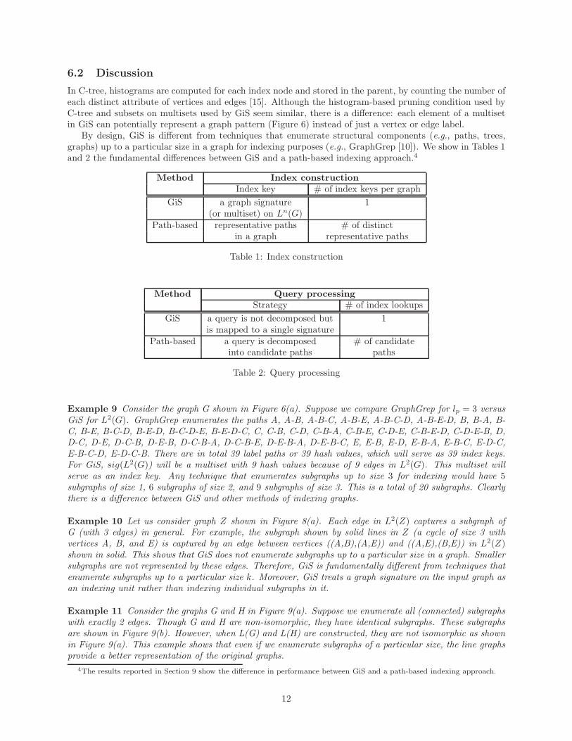
6.2 Discussion
In C-tree, histograms are computed for each index node and stored in the parent, by counting the number ofeach distinct attribute of vertices and edges [15]. Although the histogram-based pruning condition used byC-tree and subsets on multisets used by GiS seem similar, there is a difference: each element of a multisetin GiS can potentially represent a graph pattern (Figure 6) instead of just a vertex or edge label.
By design, GiS is different from techniques that enumerate structural components (e.g., paths, trees,graphs) up to a particular size in a graph for indexing purposes (e.g., GraphGrep [10]). We show in Tables 1and 2 the fundamental differences between GiS and a path-based indexing approach.4
Method Index constructionIndex key # of index keys per graph
GiS a graph signature 1(or multiset) on Ln(G)
Path-based representative paths # of distinctin a graph representative paths
Table 1: Index construction
Method Query processingStrategy # of index lookups
GiS a query is not decomposed but 1is mapped to a single signature
Path-based a query is decomposed # of candidateinto candidate paths paths
Table 2: Query processing
Example 9 Consider the graph G shown in Figure 6(a). Suppose we compare GraphGrep for lp = 3 versusGiS for L2(G). GraphGrep enumerates the paths A, A-B, A-B-C, A-B-E, A-B-C-D, A-B-E-D, B, B-A, B-C, B-E, B-C-D, B-E-D, B-C-D-E, B-E-D-C, C, C-B, C-D, C-B-A, C-B-E, C-D-E, C-B-E-D, C-D-E-B, D,D-C, D-E, D-C-B, D-E-B, D-C-B-A, D-C-B-E, D-E-B-A, D-E-B-C, E, E-B, E-D, E-B-A, E-B-C, E-D-C,E-B-C-D, E-D-C-B. There are in total 39 label paths or 39 hash values, which will serve as 39 index keys.For GiS, sig(L2(G)) will be a multiset with 9 hash values because of 9 edges in L2(G). This multiset willserve as an index key. Any technique that enumerates subgraphs up to size 3 for indexing would have 5subgraphs of size 1, 6 subgraphs of size 2, and 9 subgraphs of size 3. This is a total of 20 subgraphs. Clearlythere is a difference between GiS and other methods of indexing graphs.
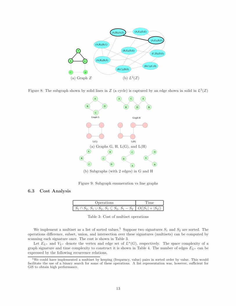
Example 10 Let us consider graph Z shown in Figure 8(a). Each edge in L2(Z) captures a subgraph ofG (with 3 edges) in general. For example, the subgraph shown by solid lines in Z (a cycle of size 3 withvertices A, B, and E) is captured by an edge between vertices ((A,B),(A,E)) and ((A,E),(B,E)) in L2(Z)shown in solid. This shows that GiS does not enumerate subgraphs up to a particular size in a graph. Smallersubgraphs are not represented by these edges. Therefore, GiS is fundamentally different from techniques thatenumerate subgraphs up to a particular size k. Moreover, GiS treats a graph signature on the input graph asan indexing unit rather than indexing individual subgraphs in it.
Example 11 Consider the graphs G and H in Figure 9(a). Suppose we enumerate all (connected) subgraphswith exactly 2 edges. Though G and H are non-isomorphic, they have identical subgraphs. These subgraphsare shown in Figure 9(b). However, when L(G) and L(H) are constructed, they are not isomorphic as shownin Figure 9(a). This example shows that even if we enumerate subgraphs of a particular size, the line graphsprovide a better representation of the original graphs.
4The results reported in Section 9 show the difference in performance between GiS and a path-based indexing approach.
12
A
B
C D
E
(A,B),(A,E)
(A,B),(B,C)
(A,B),(B,E)
(B,C),(B,E)(B,C),(C,D)
(B,E),(D,E)(C,D),(D,E)
(A,E),(B,E)
(A,E),(D,E)
(a) Graph Z (b) L2(Z)
Figure 8: The subgraph shown by solid lines in Z (a cycle) is captured by an edge shown in solid in L2(Z)
A
Graph G
L(G)
B
C
D
A
B
C
D
A
B
Graph H
L(H)
(a) Graphs G, H, L(G), and L(H)
C
D
A
D
A
B
A
B
C
B
C
D
(b) Subgraphs (with 2 edges) in G and H
Figure 9: Subgraph enumeration vs line graphs
6.3 Cost Analysis
Operations Time
S1 ∩ S2, S1 ∪ S2, S1 ⊆ S2, S1 − S2 O(|S1|+ |S2|)
Table 3: Cost of multiset operations
We implement a multiset as a list of sorted values.5 Suppose two signatures S1 and S2 are sorted. Theoperations difference, subset, union, and intersection over these signatures (multisets) can be computed byscanning each signature once. The cost is shown in Table 3.
Let ELn and VLn denote the vertex and edge set of Ln(G), respectively. The space complexity of agraph signature and time complexity to construct it is shown in Table 4. The number of edges ELn can beexpressed by the following recurrence relations,
5We could have implemented a multiset by keeping (frequency, value) pairs in sorted order by value. This wouldfacilitate the use of a binary search for some of these operations. A list representation was, however, sufficient forGiS to obtain high performance.
13
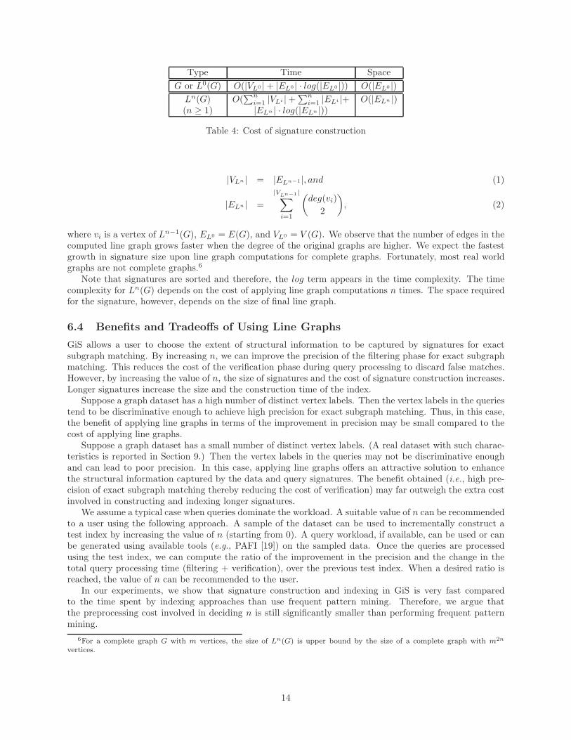
Type Time Space
G or L0(G) O(|VL0 |+ |EL0 | · log(|EL0 |)) O(|EL0 |)
Ln(G) O(∑n
i=1 |VLi |+∑n
i=1 |ELi |+ O(|ELn |)(n ≥ 1) |ELn | · log(|ELn |))
Table 4: Cost of signature construction
|VLn | = |ELn−1 |, and (1)
|ELn | =
|VLn−1 |∑
i=1
(
deg(vi)
2
)
, (2)
where vi is a vertex of Ln−1(G), EL0 = E(G), and VL0 = V (G). We observe that the number of edges in thecomputed line graph grows faster when the degree of the original graphs are higher. We expect the fastestgrowth in signature size upon line graph computations for complete graphs. Fortunately, most real worldgraphs are not complete graphs.6
Note that signatures are sorted and therefore, the log term appears in the time complexity. The timecomplexity for Ln(G) depends on the cost of applying line graph computations n times. The space requiredfor the signature, however, depends on the size of final line graph.
6.4 Benefits and Tradeoffs of Using Line Graphs
GiS allows a user to choose the extent of structural information to be captured by signatures for exactsubgraph matching. By increasing n, we can improve the precision of the filtering phase for exact subgraphmatching. This reduces the cost of the verification phase during query processing to discard false matches.However, by increasing the value of n, the size of signatures and the cost of signature construction increases.Longer signatures increase the size and the construction time of the index.
Suppose a graph dataset has a high number of distinct vertex labels. Then the vertex labels in the queriestend to be discriminative enough to achieve high precision for exact subgraph matching. Thus, in this case,the benefit of applying line graphs in terms of the improvement in precision may be small compared to thecost of applying line graphs.
Suppose a graph dataset has a small number of distinct vertex labels. (A real dataset with such charac-teristics is reported in Section 9.) Then the vertex labels in the queries may not be discriminative enoughand can lead to poor precision. In this case, applying line graphs offers an attractive solution to enhancethe structural information captured by the data and query signatures. The benefit obtained (i.e., high pre-cision of exact subgraph matching thereby reducing the cost of verification) may far outweigh the extra costinvolved in constructing and indexing longer signatures.
We assume a typical case when queries dominate the workload. A suitable value of n can be recommendedto a user using the following approach. A sample of the dataset can be used to incrementally construct atest index by increasing the value of n (starting from 0). A query workload, if available, can be used or canbe generated using available tools (e.g., PAFI [19]) on the sampled data. Once the queries are processedusing the test index, we can compute the ratio of the improvement in the precision and the change in thetotal query processing time (filtering + verification), over the previous test index. When a desired ratio isreached, the value of n can be recommended to the user.
In our experiments, we show that signature construction and indexing in GiS is very fast comparedto the time spent by indexing approaches than use frequent pattern mining. Therefore, we argue thatthe preprocessing cost involved in deciding n is still significantly smaller than performing frequent patternmining.
6For a complete graph G with m vertices, the size of Ln(G) is upper bound by the size of a complete graph with m2n
vertices.
14
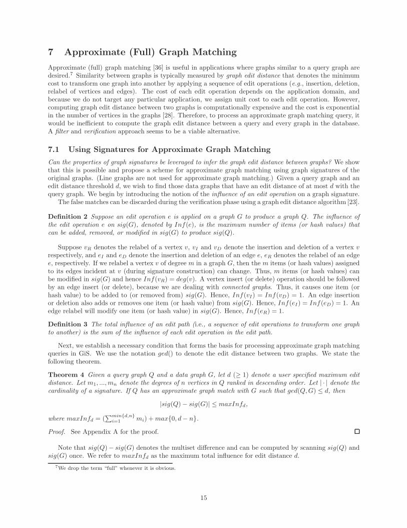
7 Approximate (Full) Graph Matching
Approximate (full) graph matching [36] is useful in applications where graphs similar to a query graph aredesired.7 Similarity between graphs is typically measured by graph edit distance that denotes the minimumcost to transform one graph into another by applying a sequence of edit operations (e.g., insertion, deletion,relabel of vertices and edges). The cost of each edit operation depends on the application domain, andbecause we do not target any particular application, we assign unit cost to each edit operation. However,computing graph edit distance between two graphs is computationally expensive and the cost is exponentialin the number of vertices in the graphs [28]. Therefore, to process an approximate graph matching query, itwould be inefficient to compute the graph edit distance between a query and every graph in the database.A filter and verification approach seems to be a viable alternative.
7.1 Using Signatures for Approximate Graph Matching
Can the properties of graph signatures be leveraged to infer the graph edit distance between graphs? We showthat this is possible and propose a scheme for approximate graph matching using graph signatures of theoriginal graphs. (Line graphs are not used for approximate graph matching.) Given a query graph and anedit distance threshold d, we wish to find those data graphs that have an edit distance of at most d with thequery graph. We begin by introducing the notion of the influence of an edit operation on a graph signature.
The false matches can be discarded during the verification phase using a graph edit distance algorithm [23].
Definition 2 Suppose an edit operation e is applied on a graph G to produce a graph Q. The influence ofthe edit operation e on sig(G), denoted by Inf(e), is the maximum number of items (or hash values) thatcan be added, removed, or modified in sig(G) to produce sig(Q).
Suppose vR denotes the relabel of a vertex v, vI and vD denote the insertion and deletion of a vertex v
respectively, and eI and eD denote the insertion and deletion of an edge e, eR denotes the relabel of an edgee, respectively. If we relabel a vertex v of degree m in a graph G, then the m items (or hash values) assignedto its edges incident at v (during signature construction) can change. Thus, m items (or hash values) canbe modified in sig(G) and hence Inf(vR) = deg(v). A vertex insert (or delete) operation should be followedby an edge insert (or delete), because we are dealing with connected graphs. Thus, it causes one item (orhash value) to be added to (or removed from) sig(G). Hence, Inf(vI) = Inf(vD) = 1. An edge insertionor deletion also adds or removes one item (or hash value) from sig(G). Hence, Inf(eI) = Inf(eD) = 1. Anedge relabel will modify one item (or hash value) in sig(G). Hence, Inf(eR) = 1.
Definition 3 The total influence of an edit path (i.e., a sequence of edit operations to transform one graphto another) is the sum of the influence of each edit operation in the edit path.
Next, we establish a necessary condition that forms the basis for processing approximate graph matchingqueries in GiS. We use the notation ged() to denote the edit distance between two graphs. We state thefollowing theorem.
Theorem 4 Given a query graph Q and a data graph G, let d (≥ 1) denote a user specified maximum editdistance. Let m1, ...,mn denote the degrees of n vertices in Q ranked in descending order. Let | · | denote thecardinality of a signature. If Q has an approximate graph match with G such that ged(Q,G) ≤ d, then
|sig(Q)− sig(G)| ≤ maxInfd,
where maxInfd = (∑min{d,n}
i=1 mi) +max{0, d− n}.
Proof. See Appendix A for the proof.
Note that sig(Q)− sig(G) denotes the multiset difference and can be computed by scanning sig(Q) andsig(G) once. We refer to maxInfd as the maximum total influence for edit distance d.
7We drop the term “full” whenever it is obvious.
15

Inf(vR) Inf(veI ) Inf(veD) Inf(eI ) Inf(eD) Inf(eR)
deg(v) 1 1 1 1 1
Table 5: Influence of edit operations
7.2 Tighter Bound Computation
To compute a tighter bound for |sig(Q) − sig(G)| in Theorem 4, we replace vI and vD by two new editoperations, namely, veI and veD, respectively. We define them as follows: veI (or veD) is the insertion (ordeletion) of a vertex v followed by the insertion (or deletion) of the edge e incident on v. If a user specifiesan upper bound on the number of each edit operation, we can compute a more precise value for maxInfd.Suppose cvR , cveI , cveD , ceI , ceD , and ceR denote the upper bounds for each of the six edit operations,respectively. (Note that cvR ≤ d.) Now the allowed edit distance for approximate graph matching is:
d = cvR + 2× cveI + 2× cveD + ceI + ceD + ceR (3)
The factor of 2 is necessary for veD and veI , because each constitutes an edit operation on a vertex and anedge. The influence of each edit operation is shown in Table 5. The following value of maxInfd will be usedin Theorem 4.
maxInfd =
cvR∑
i=1
mi +
cveI+cveD+ceI+ceD+ceR∑
i=1
1 (4)
Essentially, in the RHS of Equation 4, we maximize the influence of each edit operation by using Table 5.
7.3 Signature-Cardinality Test
Theorem 4 provides a necessary condition. Interestingly, we can discard some false matches by focusing onthe difference in the cardinality of a data graph signature and a query signature. This is because the term|sig(Q)− sig(G)| in Theorem 4 is oblivious of the actual cardinality of sig(G). One scenario that may arisedue to this is as follows: G is output as a match when Q is a subgraph of G but G is a much larger graphthan Q.
We propose the Signature-Cardinality test to overcome the above problem. Suppose we do not know thebounds on the edit operations, then our test is defined as follows:
|sig(G)| − |sig(Q)| ≤d
∑
i=1
1 (5)
|sig(Q)| − |sig(G)| ≤d
∑
i=1
1 (6)
The intuition is as follows. Among the different edit operations, d edge deletes can maximize the term|sig(G)| − |sig(Q)|. But if this term exceeds the RHS value in Equation 5, then clearly ged(G,Q) > d.Similarly, d edge inserts can maximize the term |sig(Q)| − |sig(G)|. But if this term exceeds the RHS valuein Equation 6, then clearly ged(G,Q) > d.
Suppose we know the bounds on the edit operations, then we our test is defined as follows:
|sig(G)| − |sig(Q)| ≤
cveD∑
i=1
1 +
ceD∑
i=1
1 (7)
|sig(Q)| − |sig(G)| ≤
cveI∑
i=1
1 +
ceI∑
i=1
1. (8)
The intuition is that the edit operations veD and eD when applied to G remove one item from sig(G).Therefore, if |sig(G)| − |sig(Q)| exceeds the RHS value in Equation 7, then clearly we need more veD or eD
16

graph idgraph signature
union of signaturesRoot
Leaf
Figure 10: Graph signature index
edit operations to transform G to Q. This would make ged(G,Q) > d. Similarly, veI and eI edit operationscan add one item to sig(Q). Therefore, if |sig(Q)| − |sig(G)| exceeds the RHS value in Equation 8, thenclearly we need more veI and eI edit operations to transform G to Q. This would again make ged(G,Q) > d.
7.4 Discussion
Signature-Cardinality test is applied between the query signature and the data graph signature. Because webuild a hierarchical index on the data graph signatures (Section 8), this test is applied only in the leaf nodesof the index.
Line graphs are not used for approximate graph matching. This is because the influence value of an editoperation increases if L(G) is used.
8 Graph Signature Index
In this section, we describe an index structure for graph signatures (i.e., multisets) for processing exact sub-graph matching and approximate graph matching queries. Because we are dealing with multisets and performoperations on them, prior techniques for set indexing cannot be employed directly (e.g., RD-tree [16]).
8.1 Overview
We develop a disk-based index over graph signatures so that the necessary conditions described in theprevious section can be tested quickly over a large number of graph signatures during query processing. Ourgraph signature index can be conveniently implemented using available database tools that support variablelength records (e.g., Berkeley DB8).
The graph signature index is similar to an R-tree [12] in the sense that it hierarchically groups similarsignatures together, just like an R-tree that hierarchically groups nearby rectangles together. Each non-leafindex node contains (sig, ptr) entries where sig denotes a multiset, and ptr denotes a reference to a childindex node. Each leaf node also contains (sig, ptr) entries where sig denotes a graph signature, and ptr
denotes a graph id. 9 The multiset in a non-leaf node entry denotes the union of the signatures in the childnode pointed by the entry. Figure 10 shows an illustration of the graph signature index.
The following remarks highlight the pruning power of our index during query processing.
remark 5 Suppose sigp denotes the signature value in a node’s entry and sigc denotes the signature value inthe child node pointed to by the node’s entry. If a query signature is a subset of sigc, then the query signatureis also a subset of sigp. This property allows us to prune the search space of signatures while processing exactsubgraph matching queries.
remark 6 If the cardinality of the (multiset) difference between a query signature and sigc is at most somenon-negative value k, then the cardinality of the multiset difference between the query and sigp is also atmost k. (This is because sigc ⊆ sigp.) This property allows us to prune the search space of signatures whileprocessing approximate graph matching queries.
8http://www.oracle.com/technology/products/berkeley-db9Because signatures are of variable lengths, each entry in the index node can instead contain a (recid, ptr), where the recid
denotes the id of the signature stored in a heap file.
17
Algorithm 3: Exact subgraph matching
proc exactSubgraph(nodeId, sigQ)/* nodeId - index node id; sigQ - query signature; */
1 (nodetype, S)← fetchNode(nodeId) /* read node */2 foreach (sig, ptr) in S do3 if sigQ ⊆ sig then4 if nodetype = LEAF then5 Output ptr as a candidate match
else6 exactSubgraph(ptr, sigQ) /* Traverse child */
end if
end if
end foreachendproc
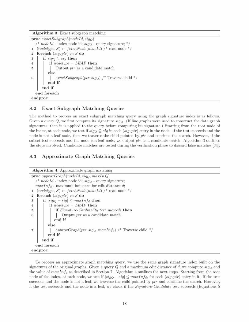
8.2 Exact Subgraph Matching Queries
The method to process an exact subgraph matching query using the graph signature index is as follows.Given a query Q, we first compute its signature sigQ. (If line graphs were used to construct the data graphsignatures, then it is applied to the query before computing its signature.) Starting from the root node ofthe index, at each node, we test if sigQ ⊆ sig in each (sig, ptr) entry in the node. If the test succeeds and thenode is not a leaf node, then we traverse the child pointed by ptr and continue the search. However, if thesubset test succeeds and the node is a leaf node, we output ptr as a candidate match. Algorithm 3 outlinesthe steps involved. Candidate matches are tested during the verification phase to discard false matches [34].
8.3 Approximate Graph Matching Queries
Algorithm 4: Approximate graph matching
proc approxGraph(nodeId, sigQ,maxInfd)/* nodeId - index node id; sigQ - query signature;maxInfd - maximum influence for edit distance d;
1 (nodetype, S)← fetchNode(nodeId) /* read node */2 foreach (sig, ptr) in S do3 if |sigQ − sig| ≤ maxInfd then4 if nodetype = LEAF then5 if Signature-Cardinality test succeeds then6 Output ptr as a candidate match
end if
else7 approxGraph(ptr, sigQ,maxInfd) /* Traverse child */
end if
end if
end foreachendproc
To process an approximate graph matching query, we use the same graph signature index built on thesignatures of the original graphs. Given a query Q and a maximum edit distance of d, we compute sigQ andthe value of maxInfd as described in Section 7. Algorithm 4 outlines the next steps. Starting from the rootnode of the index, at each node, we test if |sigQ− sig| ≤ maxInfd, for each (sig, ptr) entry in it. If the testsucceeds and the node is not a leaf, we traverse the child pointed by ptr and continue the search. However,if the test succeeds and the node is a leaf, we check if the Signature-Candidate test succeeds (Equations 5
18

Algorithm 5: Bulk loading a Signature Index
Global: int i = 1;proc bulkLoad(DList, k, f)/* DList - signature list; k - a positive integer; f - fanout */
1 Suppose idx denotes the index position of a signature s in DList. Create SList by sorting (idx, |s|)for each s ∈ DList
2 split(DList, k, f , SList)3 Create upper level index nodes with increasing node ids containing k (sig, ptr) entries (or less for thelast index node) by grouping k lower level nodes in the order of their node ids. Each sig value in anode’s entry is the union of the signatures in the lower level node.
4 Repeat Line 3 till the upper level has only one index node i.e., root.endprocproc split(DList, k, f , SList)5 Among the k highest cardinality signatures in sList find the pair that is most dissimilar6 Let sA and sB denote the two seed signatures from groups A and B7 Let sUA and sUB denote the union of the signatures in each group8 foreach s ∈ DList do
9 if |s∩sUA||s∪sUA| >
|s∩sUB ||s∪sUB | then
10 add s to group A and update sUA
else
11 if |s∩sUA||s∪sUA| <
|s∩sUB ||s∪sUB | then
12 add s to group B and update sUB
else13 add s to the group with fewer signatures and update its union
end if
end if
end foreach14 if A has more than f signatures then15 create SListA for signatures in A16 split(A, k, f , SListA)
else17 create leaf index node i containing the signatures in A18 i← i+ 1
end if19 if B has more than f signatures then20 create SListB for signatures in B21 split(B, k, f , SListB)
else22 create leaf index node i containing the signatures in B23 i← i+ 1
end ifendproc
and 6). If so, we output ptr as a candidate match. Candidate matches are tested during the verificationphase to discard false matches by computing graph edit distance [23].
If the upper bounds on edit operations are available, then we computemaxInfd using Equation 4. For theSignature-Cardinality test, we use Equations 7 and 8. Note that we do not apply the Signature-Cardinalitytest when non-leaf nodes are searched, because the signatures in these nodes are constructed by computingthe union of the child node signatures.
19

8.4 Bulk Loading the Index
We propose a bulk-loading algorithm to speed up the indexing process rather than inserting one signature ata time into the index. Algorithm 5 outlines the steps involved. Given a group of input graph signatures, werecursively split the group into two groups, until each group has at most f signatures, where f is the desirednode fanout. For a group, we start by picking two dissimilar seeds. Similarity between two signatures
is defined as follows: Given two signatures S1 and S2, their similarity is given by |S1∩S2||S1∪S2|
. Rather than
computing the similarity over all possible pairs to select the seeds, we only examine the k highest cardinalitysignatures. The intuition is that if two signatures with high cardinalities share the least number of elements,then the remaining signatures may be more likely to be similar to either one of them.
Each group is initialized with a seed signature and the union (∪) of the signatures in each group ismaintained. Each remaining graph signature is assigned to the group whose union of signatures has thehighest similarity with the graph signature. In case of ties, we assign the signature to the group with fewersignatures. If a group has more than f signatures, it is split again. Otherwise, the group forms a leaf node.Each time a leaf is created, it is assigned an id one greater than the id assigned to a previously created leafnode. Once all the leaf index nodes are created, we are ready to create the upper level nodes in a bottom-upfashion.
Starting with the node with the smallest id, we group f lower level nodes in the order of their ids tocreate an upper level node. Each entry contains the union of the signatures in a lower level node and thenode’s id. The upper level nodes are also assigned increasing ids as they are created. We continue creatingupper level nodes until only one upper level node is required, i.e., the root of the index. The ids assigned tothe index nodes resemble a reverse of breath first search ordering.
The design of the index in GiS draws inspiration from the psiX system [27].
8.5 Discussion
One may wonder if a graph signature can be inserted or deleted from the graph signature index, i.e.,a dynamic index. It is possible to design an insertion algorithm in similar vein to an R-tree’s insertionalgorithm. The best child can be picked by comparing the similarity of the input signature with the signaturein a node’s entry. The entry with the highest similarity to the input signature can be chosen for insertion.(This is analogous to choosing the bounding box that requires the least increase in size in an R-tree.) Oncethe signature is inserted into a leaf node, the upper level node entries can be updated with the new unionof the signatures in a child node. If a node split is necessary, an approach similar to the quadratic splittingalgorithm of an R-tree can be designed, wherein signatures are considered instead of bounding rectangles.Similarly, we can design an approach for the deletion of a signature. Note that the insertion and deletionalgorithms have not been implemented in GiS and we consider this as future work.
9 Performance Evaluation
In this section, we present the performance evaluation of GiS. We focus on queries with high selectivities,and therefore, consider queries whose processing cost is not dominated by the cost of verification [34].
9.1 Techniques Considered for Performance Evaluation
We compared GiS with recent techniques for exact subgraph matching namely, FG-index, C-tree, and SING.Recall that FG-index uses mining for extracting features for indexing and store part of the index in main-memory and part on disk. C-tree does not rely on mining but the implementation is main-memory based.SING is also main-memory based, does not use mining, and extracts paths in graphs as features for indexing.For fairness of comparison, we measured SING’s performance for finding the first occurrence of an exactsubgraph match when comparing with GiS. SING has shown to be superior to recent techniques such asGCoding [48] and Tree+∆ [47], and hence we do not consider them in our study. SING has also shown to besuperior to C-tree on large graphs. Note that techniques such as FG-index, C-tree, Tree+∆, and GCodingwere designed for small graphs.
20
For approximate (full) graph matching, we compared the performance of GiS with range queries supportedby C-tree. We also compared the read cost of APPFULL with the filtering time of GiS. APPFULL scansevery graph in the database during query processing. While GiS is not designed for approximate subgraphmatching, we compared it with TALE, a disk-based technique for approximate subgraph matching of largegraphs, to gain insights into the scalability of GiS, which is also disk-based.
We did not use the iGraph framework [13] because it was developed for MS Windows. Instead we usedthe original implementation from the authors of FG-index, C-tree, SING, and TALE.
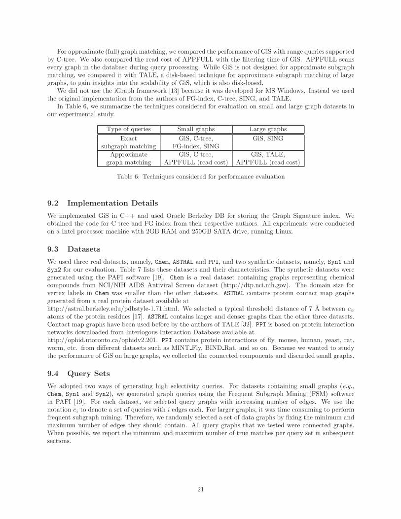
In Table 6, we summarize the techniques considered for evaluation on small and large graph datasets inour experimental study.
Type of queries Small graphs Large graphs
Exact GiS, C-tree, GiS, SINGsubgraph matching FG-index, SING
Approximate GiS, C-tree, GiS, TALE,graph matching APPFULL (read cost) APPFULL (read cost)
Table 6: Techniques considered for performance evaluation
9.2 Implementation Details
We implemented GiS in C++ and used Oracle Berkeley DB for storing the Graph Signature index. Weobtained the code for C-tree and FG-index from their respective authors. All experiments were conductedon a Intel processor machine with 2GB RAM and 250GB SATA drive, running Linux.
9.3 Datasets
We used three real datasets, namely, Chem, ASTRAL and PPI, and two synthetic datasets, namely, Syn1 andSyn2 for our evaluation. Table 7 lists these datasets and their characteristics. The synthetic datasets weregenerated using the PAFI software [19]. Chem is a real dataset containing graphs representing chemicalcompounds from NCI/NIH AIDS Antiviral Screen dataset (http://dtp.nci.nih.gov). The domain size forvertex labels in Chem was smaller than the other datasets. ASTRAL contains protein contact map graphsgenerated from a real protein dataset available athttp://astral.berkeley.edu/pdbstyle-1.71.html. We selected a typical threshold distance of 7 A between cαatoms of the protein residues [17]. ASTRAL contains larger and denser graphs than the other three datasets.Contact map graphs have been used before by the authors of TALE [32]. PPI is based on protein interactionnetworks downloaded from Interlogous Interaction Database available athttp://ophid.utoronto.ca/ophidv2.201. PPI contains protein interactions of fly, mouse, human, yeast, rat,worm, etc. from different datasets such as MINT Fly, BIND Rat, and so on. Because we wanted to studythe performance of GiS on large graphs, we collected the connected components and discarded small graphs.
9.4 Query Sets
We adopted two ways of generating high selectivity queries. For datasets containing small graphs (e.g.,Chem, Syn1 and Syn2), we generated graph queries using the Frequent Subgraph Mining (FSM) softwarein PAFI [19]. For each dataset, we selected query graphs with increasing number of edges. We use thenotation ei to denote a set of queries with i edges each. For larger graphs, it was time consuming to performfrequent subgraph mining. Therefore, we randomly selected a set of data graphs by fixing the minimum andmaximum number of edges they should contain. All query graphs that we tested were connected graphs.When possible, we report the minimum and maximum number of true matches per query set in subsequentsections.
21

Dataset Total # # of # of # ofname of vertices edges unique
graphs vertexMax Avg Max Avg labels
(domainsize)
Syn1 80,000 30 12 33 13 235Syn2 80,000 36 17 42 21 180Chem 40,000 183 23 189 25 38
ASTRAL 34,810 904 174 3,677 686 106PPI 70 4,697 1,235 16,849 3,342 35,203
Table 7: Datasets and their characteristics
Syn1/L(G) Syn2/L(G) ASTRAL/L(G) PPI/L(G)
# of 80,000 80,000 34,810 70graphsAvg. 73.3 bytes 129.9 bytes 20.6 KB 333.7 KBsizeAvg. 53.8 µsecs 92.6 µsecs 19.6 msecs 341 msecstime
Table 8: Average signature size and construction time
9.5 Evaluation Metrics
To evaluate the indexing performance, we measured (a) the total wall clock time to build the index and (b)the index size, for varying number of input data graphs.
Because the code provided by the authors of FG-index did not output the number of candidates or thefiltering time, we compared GiS and FG-index during query processing by measuring the average wall clocktime to process a query, which included both the filtering and verification costs. To compare C-tree and GiS,we measured (a) the average wall clock time per query for the filtering phase and (b) the average precisionachieved per query (i.e., the pruning power). Suppose cand and true denote the candidate set and the set
of true matches, respectively. We compute precision p = |true||cand| because recall is always 1. We also measured
average precision and average filtering time for approximate graph matching queries.We measured the cost of constructing graph signatures and the cost and benefit of using line graphs. We
started with a cold file system buffer cache before beginning both the indexing and query processing tasks.
9.6 Cost of Constructing Graph Signatures
Table 8 shows the average size of a graph signature and the average time to construct a signature for Syn1,Syn2, ASTRAL, and PPI. One line graph computation was applied on these datasets. As ASTRAL containedlarge, dense graphs, the construction time and signature size were larger than that for Syn1 and Syn2. PPIcontained the largest graphs and therefore, the average construction time and signature size were higherthan the rest. Table 9 shows the signature construction costs for Chem. Up to two line graph computationswere employed. Although, L(L(G)) increased the average signature size by three times, the benefit in termsof improved precision of exact subgraph matching was significant. (See Section 9.9 for precision results.)The above results demonstrate that graph signatures can be constructed very efficiently.
Chem G L(G) L(L(G))
# of graphs 40,000 40,000 40,000Avg. size 90.33 bytes 128.77 bytes 274.57 bytesAvg. time 40.00 µsecs 57.50 µsecs 134.25 µsecs
Table 9: Average signature size and construction time
22
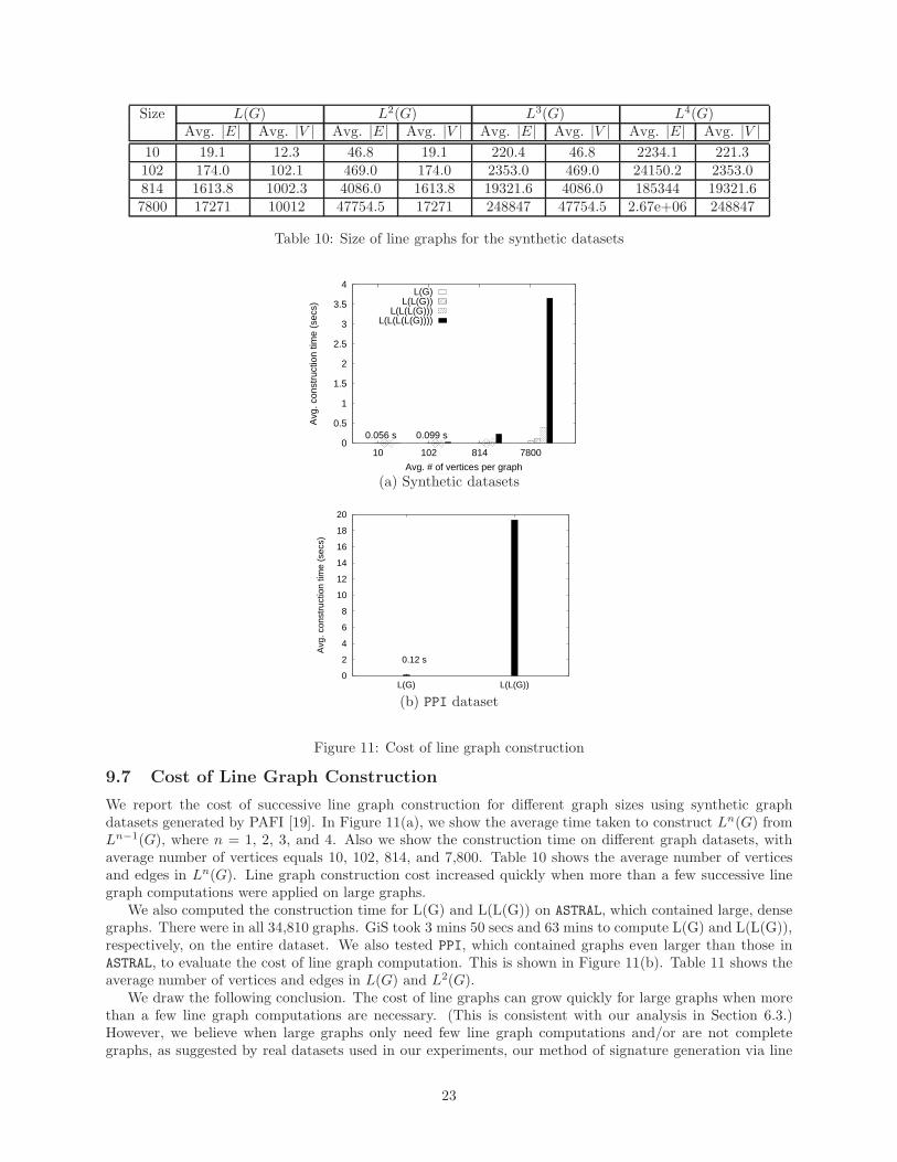
Size L(G) L2(G) L3(G) L4(G)Avg. |E| Avg. |V | Avg. |E| Avg. |V | Avg. |E| Avg. |V | Avg. |E| Avg. |V |
10 19.1 12.3 46.8 19.1 220.4 46.8 2234.1 221.3102 174.0 102.1 469.0 174.0 2353.0 469.0 24150.2 2353.0814 1613.8 1002.3 4086.0 1613.8 19321.6 4086.0 185344 19321.67800 17271 10012 47754.5 17271 248847 47754.5 2.67e+06 248847
Table 10: Size of line graphs for the synthetic datasets
0
0.5
1
1.5
2
2.5
3
3.5
4
10 102 814 7800
Avg
. con
stru
ctio
n tim
e (s
ecs)
Avg. # of vertices per graph
0.056 s 0.099 s
L(G)L(L(G))
L(L(L(G)))L(L(L(L(G))))
(a) Synthetic datasets
0
2
4
6
8
10
12
14
16
18
20
L(G) L(L(G))
Avg
. con
stru
ctio
n tim
e (s
ecs)
0.12 s
(b) PPI dataset
Figure 11: Cost of line graph construction
9.7 Cost of Line Graph Construction
We report the cost of successive line graph construction for different graph sizes using synthetic graphdatasets generated by PAFI [19]. In Figure 11(a), we show the average time taken to construct Ln(G) fromLn−1(G), where n = 1, 2, 3, and 4. Also we show the construction time on different graph datasets, withaverage number of vertices equals 10, 102, 814, and 7,800. Table 10 shows the average number of verticesand edges in Ln(G). Line graph construction cost increased quickly when more than a few successive linegraph computations were applied on large graphs.
We also computed the construction time for L(G) and L(L(G)) on ASTRAL, which contained large, densegraphs. There were in all 34,810 graphs. GiS took 3 mins 50 secs and 63 mins to compute L(G) and L(L(G)),respectively, on the entire dataset. We also tested PPI, which contained graphs even larger than those inASTRAL, to evaluate the cost of line graph computation. This is shown in Figure 11(b). Table 11 shows theaverage number of vertices and edges in L(G) and L2(G).
We draw the following conclusion. The cost of line graphs can grow quickly for large graphs when morethan a few line graph computations are necessary. (This is consistent with our analysis in Section 6.3.)However, we believe when large graphs only need few line graph computations and/or are not completegraphs, as suggested by real datasets used in our experiments, our method of signature generation via line
23

Number of graphs0 20000 40000 60000 80000
Tot
al ti
me
(sec
s)
20
40
60
80
Syn1
Syn2
Syn1
Syn2
Syn1
Syn2
GiS (L(G))
= 0.01)σFG−index (
C−tree
Number of graphs0 20000 40000 60000 80000
Inde
x si
ze (
MB
)
20
40
60
80
Syn1
Syn2
Syn1
Syn2
Syn1
Syn2
GiS (L(G))
= 0.01)σFG−index (
C−tree
Number of graphs
0 20000 40000
Tot
al ti
me
(sec
s)
1
10
210
310 GiS (L(L(G)))
GiS (L(G))
GiS (G)
C−tree
= 0.1)σFG−index(
Number of graphs0 20000 40000
Inde
x si
ze (
MB
)
10
20
30
40
50GiS (L(L(G)))
GiS (L(G))
GiS (G)
= 0.1)σFG−index (
C−tree
(a) Syn1 & Syn2 (b) Syn1 & Syn2 (c) Chem (d) Chem
Figure 12: Indexing performance (GiS, C-tree, FG-index)
graphs can still provide a practical and efficient solution.
9.8 Indexing Performance
9.8.1 Syn1, Syn2, and Chem
In this section, we present the indexing performance of GiS, C-tree, and FG-index. For FG-index, as selectedby the authors, we set the value of tolerance factor σ = 0.01 and σ = 0.1 for synthetic datasets and Chem,respectively. For fair comparison between GiS and C-tree, we built indexes with a fanout of 500.
Figure 12(a) show the total time taken for indexing the synthetic datasets for increasing number of inputgraphs. Clearly, the bulkloading approach of GiS outperformed C-tree and FG-index. FG-index incurredhigher indexing cost than GiS due to the application of frequent subgraph mining. For example, GiS was3.3 times faster than FG-index for Syn2 (80,000). Also C-tree incurred a higher cost than GiS due tothe hierarchical clustering operation. For example, GiS was 3 times faster than C-tree for Syn2 (80,000).Above all, GiS had superior scalability trends. (The timing reported for GiS included the time to constructsignatures for all the datasets.) (Memory consumption of C-tree was significantly higher than that of GiS.)
The size of indexes built by FG-index and GiS for synthetic datasets were significantly smaller than thatbuilt by C-tree. These results are shown in Figure 12(b). Although FG-index had smaller index sizes thanGiS, we show in the next section that GiS is still superior than FG-index for query processing.
Figures 12(c) and 12(d) report the indexing cost for Chem. GiS and C-tree had superior indexing perfor-mance as compared with FG-index. FG-index was about two orders of magnitude slower than GiS due tothe expensive frequent subgraph mining phase. GiS had the smallest index size even with two applications ofline graphs. It used line graphs for Chem, because this dataset had a small number of distinct vertex labels.As expected, the indexing time and index size of GiS increased with the computation of line graphs. Yet,the improvement obtained in average precision for exact subgraph matching queries was significant. (Theprecision results are presented in Section 9.9.)
We also compared the cost of indexing of GiS and SING on Syn1 (80,000 graphs), Syn2 (80,000 graphs),and Chem (40,000 graphs). SING used the default value (provided in the source code) for feature length(or path length), which yields high precision of exact subgraph matching. GiS built the index using L(G)for Syn1, L(G) for Syn2, and L(L(G)) for Chem. The index construction time and index size are shownin Figures 13(a) and 13(b), respectively. We observed that GiS was several times faster than SING in
L(G) L2(G)Avg. |E| Avg. |V | Avg. |E| Avg. |V |
83428.8 3341.97 1.19507e+07 83428.8
Table 11: Size of line graphs for PPI
24

0
100
200
300
400
Chem(L(L(G)))
Syn1(L(G))
Syn2(L(G))
Tot
al ti
me
(sec
s)
GiSSING
0
100
200
300
400
Chem(L(L(G)))
Syn1(L(G))
Syn2(L(G))
Inde
x si
ze (
MB
)
GiSSING
(a) Index construction time (b) Index size
Figure 13: Indexing performance: GiS vs SING
0
2000
4000
6000
8000
ASTRAL PPI
Tot
al ti
me
(sec
s)
Datasets
37 s743 s
GiS (L(G))SING (lp = 2)
0
200
400
600
800
1000
ASTRAL PPI
Inde
x si
ze (
MB
)
Datasets
32 MB101 MB
GiS (L(G))SING (lp = 2)
(a) Index construction time (b) Index size
Figure 14: Indexing performance of GiS and SING on ASTRAL and PPI
constructing the indexes. The size of the indexes built by GiS were smaller than those built by SING for allthe three datasets.
9.8.2 ASTRAL Dataset
ASTRAL contained large, dense graphs and our experiments on this dataset clearly demonstrates the supe-riority of GiS. GiS indexed this dataset using one line graph computation in 1,192 seconds. (Note thatthis time included the time to construct line graphs, construct signatures, and then build the index on thesignatures.) The index size was 847 MB. We set the buffer cache size in Berkeley DB to 164 MB.
Both FG-index and C-tree failed to index ASTRAL that contained large, dense graphs. FG-index crashedas it ran out of virtual memory due to very large number of frequent patterns (more than a million) for amodest setting of σ = 0.1 and σ = 0.15, which are similar to values chosen by the authors of FG-index intheir paper. Moreover, finding frequent graph patterns required more than 3 days. This clearly demonstratesthe limitation of a mining-based approach on large, dense graphs. C-tree crashed while indexing ASTRAL
even when maximum amount of memory was provided for heap space.SING, a main-memory based technique, was unable to index the entire ASTRAL dataset using the default
value of path length (or feature length) on a machine with 8 GB RAM. By design, SING stored not onlythe paths up to a particular length (along with frequency information) but also the position information offeatures for improved indexing and verification. 10 Fortunately, SING indexed the entire ASTRAL datasetsuccessfully when path length was reduced to 2. The index construction time and index size for ASTRAL areshown in Figures 14(a) and 14(b), respectively. GiS was much faster than SING, although the index size ofGiS was larger. Despite the larger index size, we show later in this section that GiS can outperform SINGfor exact subgraph matching.
10This shows that main-memory based techniques will fail on large graph datasets and emphasizes the need for disk-basedindexing techniques.
25

Avg
. res
pons
e tim
e (s
ecs)
0
0.2
0.4
0.6
GiS L(G) (Syn1) FG−index (Syn1)
12 e9 e6 e3e
GiS L(G) (Syn2) FG−index (Syn2)
Query set
Avg
. filt
erin
g tim
e (s
ecs)
0
0.1
0.2
0.3
0.4
GiS L(G) (Syn1) C−tree (Syn1)
12 e9 e6 e3e
GiS L(G) (Syn2) C−tree (Syn2)
Query set
Avg
. filt
erin
g tim
e (s
ecs)
0
0.05
0.1
0.15
0.2
GiS (G)
GiS (L(G))
GiS (L(L(G))C−tree (pseudo=5)
C−tree (pseudo=0)
5 e4 e3 eQuery set
(a) Synthetic datasets (c) Synthetic datasets (e) Chem (without edge labels)(GiS, FG-index) (GiS, C-tree) (GiS, C-tree)
Avg
. res
pons
e tim
e (s
ecs)
0
0.05
0.1
0.15
0.2FG-index
15 e12 e9 e6e
GiS (L(L(G)))
Query set
Avg
. pre
cisi
on
0
0.2
0.4
0.6
0.8
1
GiS(Syn1,L(G)) C−tree (Syn1)
GiS(Syn2,L(G)) C−tree (Syn2)
12 e9 e6 e3 eQuery set
Avg
. pre
cisi
on
0
0.2
0.4
0.6
0.8
1
5 e4 e3e
GiS (G)GiS (L(G)) GiS (L(L(G)))
C−tree (pseudo=0)
C−tree (pseudo=5)
Query set
(b) Chem (with edge labels) (d) Synthetic datasets (f) Chem (without edge labels)(GiS, FG-index) (GiS, C-tree) (GiS, C-tree)
Figure 15: Performance results of exact subgraph matching: GiS, FG-index, C-tree
9.8.3 PPI Dataset
PPI contained the largest graphs compared with other datasets. We compared the indexing performance ofGiS and SING.11 As the implementation of SING is main-memory based, it failed to index the entire dataseton a machine with 8 GB RAM using the default value of path length. So we reduced the path length to2. Further, this will enable fair comparison with GiS, which indexed this dataset using L(G). (We set theBerkeley DB buffer cache size in GiS to 164 MB.) The index construction time and index size for PPI areshown in Figures 14(a) and 14(b), respectively. GiS was faster and built a smaller index than SING.
9.9 Exact Subgraph Matching Queries
9.9.1 Syn1, Syn2, and Chem
First, we report the comparison between GiS and FG-index for processing exact subgraph matching queries.(Recall that the implementation of FG-index provided by the authors does not report the filtering time orthe candidate size and hence they are not reported here.) Figures 15(a) and 15(b) show the performancecomparison for synthetic datasets and Chem, respectively for query sets with increasing number of edges.Each query set had 20 random queries with high selectivities. For Chem, we considered the edge labels whileindexing and query processing. (Both FG-index and GiS support graphs with edge labels.)
The non-holistic approach of FG-index, which required finding partial matches for subgraphs of a query,was slower than GiS in all cases. GiS adopts a holistic approach to processing a query: the entire querygraph is considered together while searching the index. For example, GiS was 5.5 and 3.0 times faster thanFG-index for Syn2 (e12) and Chem (e12), respectively.
Next, we discuss the performance comparison of GiS and C-tree. Figures 15(c) and 15(d) show the average
11C-tree and FG-index are designed for small graphs.
26
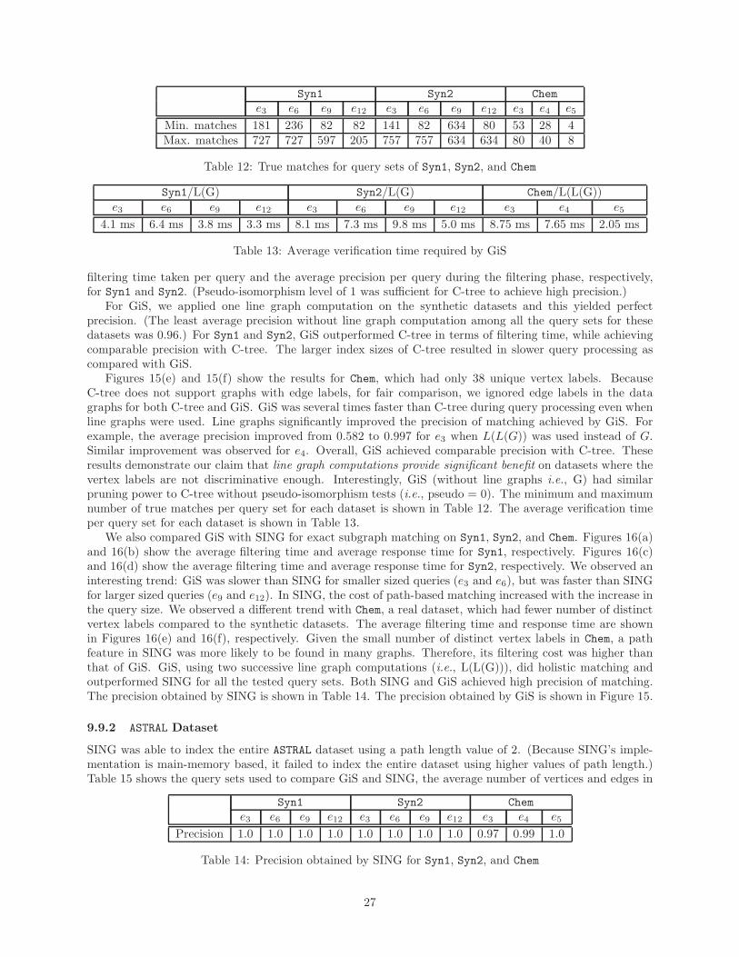
Syn1 Syn2 Chem
e3 e6 e9 e12 e3 e6 e9 e12 e3 e4 e5
Min. matches 181 236 82 82 141 82 634 80 53 28 4Max. matches 727 727 597 205 757 757 634 634 80 40 8
Table 12: True matches for query sets of Syn1, Syn2, and Chem
Syn1/L(G) Syn2/L(G) Chem/L(L(G))e3 e6 e9 e12 e3 e6 e9 e12 e3 e4 e5
4.1 ms 6.4 ms 3.8 ms 3.3 ms 8.1 ms 7.3 ms 9.8 ms 5.0 ms 8.75 ms 7.65 ms 2.05 ms
Table 13: Average verification time required by GiS
filtering time taken per query and the average precision per query during the filtering phase, respectively,for Syn1 and Syn2. (Pseudo-isomorphism level of 1 was sufficient for C-tree to achieve high precision.)
For GiS, we applied one line graph computation on the synthetic datasets and this yielded perfectprecision. (The least average precision without line graph computation among all the query sets for thesedatasets was 0.96.) For Syn1 and Syn2, GiS outperformed C-tree in terms of filtering time, while achievingcomparable precision with C-tree. The larger index sizes of C-tree resulted in slower query processing ascompared with GiS.
Figures 15(e) and 15(f) show the results for Chem, which had only 38 unique vertex labels. BecauseC-tree does not support graphs with edge labels, for fair comparison, we ignored edge labels in the datagraphs for both C-tree and GiS. GiS was several times faster than C-tree during query processing even whenline graphs were used. Line graphs significantly improved the precision of matching achieved by GiS. Forexample, the average precision improved from 0.582 to 0.997 for e3 when L(L(G)) was used instead of G.Similar improvement was observed for e4. Overall, GiS achieved comparable precision with C-tree. Theseresults demonstrate our claim that line graph computations provide significant benefit on datasets where thevertex labels are not discriminative enough. Interestingly, GiS (without line graphs i.e., G) had similarpruning power to C-tree without pseudo-isomorphism tests (i.e., pseudo = 0). The minimum and maximumnumber of true matches per query set for each dataset is shown in Table 12. The average verification timeper query set for each dataset is shown in Table 13.
We also compared GiS with SING for exact subgraph matching on Syn1, Syn2, and Chem. Figures 16(a)and 16(b) show the average filtering time and average response time for Syn1, respectively. Figures 16(c)and 16(d) show the average filtering time and average response time for Syn2, respectively. We observed aninteresting trend: GiS was slower than SING for smaller sized queries (e3 and e6), but was faster than SINGfor larger sized queries (e9 and e12). In SING, the cost of path-based matching increased with the increase inthe query size. We observed a different trend with Chem, a real dataset, which had fewer number of distinctvertex labels compared to the synthetic datasets. The average filtering time and response time are shownin Figures 16(e) and 16(f), respectively. Given the small number of distinct vertex labels in Chem, a pathfeature in SING was more likely to be found in many graphs. Therefore, its filtering cost was higher thanthat of GiS. GiS, using two successive line graph computations (i.e., L(L(G))), did holistic matching andoutperformed SING for all the tested query sets. Both SING and GiS achieved high precision of matching.The precision obtained by SING is shown in Table 14. The precision obtained by GiS is shown in Figure 15.
9.9.2 ASTRAL Dataset
SING was able to index the entire ASTRAL dataset using a path length value of 2. (Because SING’s imple-mentation is main-memory based, it failed to index the entire dataset using higher values of path length.)Table 15 shows the query sets used to compare GiS and SING, the average number of vertices and edges in
Syn1 Syn2 Chem
e3 e6 e9 e12 e3 e6 e9 e12 e3 e4 e5
Precision 1.0 1.0 1.0 1.0 1.0 1.0 1.0 1.0 0.97 0.99 1.0
Table 14: Precision obtained by SING for Syn1, Syn2, and Chem
27

0
0.05
0.1
0.15
e3 e6 e9 e12
Avg
. filt
erin
g tim
e (s
ecs)
Query sets
GiS (L(G))SING
0
0.05
0.1
0.15
e3 e6 e9 e12
Avg
. filt
erin
g tim
e (s
ecs)
Query sets
GiS (L(G))SING
0
0.01
0.02
0.03
0.04
0.05
e3 e4 e5
Avg
. filt
erin
g tim
e (s
ecs)
Query sets
GiS (L(L(G)))SING
(a) Syn1 (c) Syn2 (e) Chem (without edge labels)
0
0.05
0.1
0.15
0.2
e3 e6 e9 e12
Avg
. res
pons
e tim
e (s
ecs)
Query sets
GiS (L(G))SING
0
0.05
0.1
0.15
0.2
e3 e6 e9 e12
Avg
. res
pons
e tim
e (s
ecs)
Query sets
GiS (L(G))SING
0
0.01
0.02
0.03
0.04
0.05
e3 e4 e5
Avg
. res
pons
e tim
e (s
ecs)
Query sets
GiS (L(L(G)))SING
(b) Syn1 (d) Syn2 (f) Chem (without edge labels)
Figure 16: Performance results of exact subgraph matching: GiS, SING
Query Avg. # Avg. # # of true Avg. precisionset of vertices of edges matches GiS SING
(min, max) (L(G))
Q1 23 48 (1, 11) 0.94 0.002Q2 26 77 (1, 118) 0.95 0.034Q3 34 80 (1, 71) 0.95 0.017Q4 36 110 (1, 24) 0.97 0.057
Table 15: Query processing performance on ASTRAL (34,810 graphs)
each query set, along with the minimum and maximum number of true matches per query set. Figures 17(a)and 17(b) show the average filtering time and average response time, respectively. Clearly, GiS was severaltimes faster than SING. SING yielded poor precision of matching using path length of 2, but GiS (usingL(G)) achieved high precision of matching. These results are shown in Table 15. The average verificationtime for GiS was 141 ms, 284 ms, 131 ms, and 37 ms for query sets Q1, Q2, Q3, and Q4, respectively. Theaverage verification time for SING was much higher because of poor precision of matching.
Next, we compared GiS and SING on a smaller subset of graphs in ASTRAL, more specifically 2,000graphs. SING used the default value of path length to achieve high precision. While SING indexed thesegraphs in 1,680 secs with an index size of 2.9 GB, GiS indexed them in 35 secs with an index size of 47 MB.Figure 18(b) shows the query sets used for the evaluation. It also shows the average size of the queries ineach query set and the average response time for each query set. The minimum and maximum number oftrue matches per query set is also reported. Note that the query sets Q1, Q2, Q3, and Q4 had 5, 4, 7, and 15queries, respectively. Figure 18(a) shows the average filtering time of GiS and SING. GiS was several timesfaster than SING for all the query sets. We also measured the precision of exact subgraph matching. GiSand SING both had perfect precision for the query sets Q2, Q3, and Q4. However, for Q1 with relativelysmaller query graphs, GiS had poorer precision than SING (0.23 vs 0.87). Interestingly, the average responsetime of GiS was still better than SING as the cost of verification was small for the tested query sets.
28
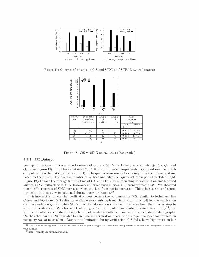
0
1
2
3
4
5
Q1 Q2 Q3 Q4A
vg. f
ilter
ing
time
(sec
s)Query set
GiS (L(G))SING (lp = 2)
0
2
4
6
8
10
Q1 Q2 Q3 Q4
Avg
. res
pons
e tim
e (s
ecs)
Query set
GiS (L(G))SING (lp = 2)
(a) Avg. filtering time (b) Avg. response time
Figure 17: Query performance of GiS and SING on ASTRAL (34,810 graphs)
0 1 2 3 4 5 6 7 8 9
10 11
Q1 Q2 Q3 Q4
Avg
. filt
erin
g tim
e (s
ecs)
GiSSING
(a)Query # of true Avg # Avg # Avg.set matches of of response
(min, max) vertices edges timeGiS SINGL(G)
Q1 (1, 22) 9 14 0.66 s 3.13 sQ2 (1, 2) 23 50 0.64 s 9.23 sQ3 (1, 11) 27 79 0.45 s 11.76 sQ4 (1, 11) 28 85 0.25 s 6.10 s
(b)
Figure 18: GiS vs SING on ASTRAL (2,000 graphs)
9.9.3 PPI Dataset
We report the query processing performance of GiS and SING on 4 query sets namely, Q1, Q2, Q3, andQ4. (See Figure 19(b).) (These contained 70, 5, 8, and 12 queries, respectively.) GiS used one line graphcomputation on the data graphs (i.e., L(G)). The queries were selected randomly from the original datasetbased on their sizes. The average number of vertices and edges per query set are reported in Table 19(b).Figure 19(a) shows the average filtering time of GiS and SING. It is interesting to note that on smaller-sizedqueries, SING outperformed GiS. However, on larger-sized queries, GiS outperformed SING. We observedthat the filtering cost of SING increased when the size of the queries increased. This is because more features(or paths) in a query were examined during query processing.12
It is interesting to note that verification cost became the bottleneck for GiS. Similar to techniques likeC-tree and FG-index, GiS relies on available exact subgraph matching algorithms [34] for the verificationstep on candidate graphs, while SING uses the information stored with features from the filtering step tospeed up verification. We observed that using VFLib, a popular exact subgraph matching library13, theverification of an exact subgraph match did not finish even after an hour on certain candidate data graphs.On the other hand, SING was able to complete the verification phase; the average time taken for verificationper query was at most 60 ms. Despite this limitation during verification, GiS did achieve high precision like
12While the filtering cost of SING increased when path length of 3 was used, its performance trend in comparison with GiSwas similar.
13http://amalfi.dis.unina.it/graph/
29
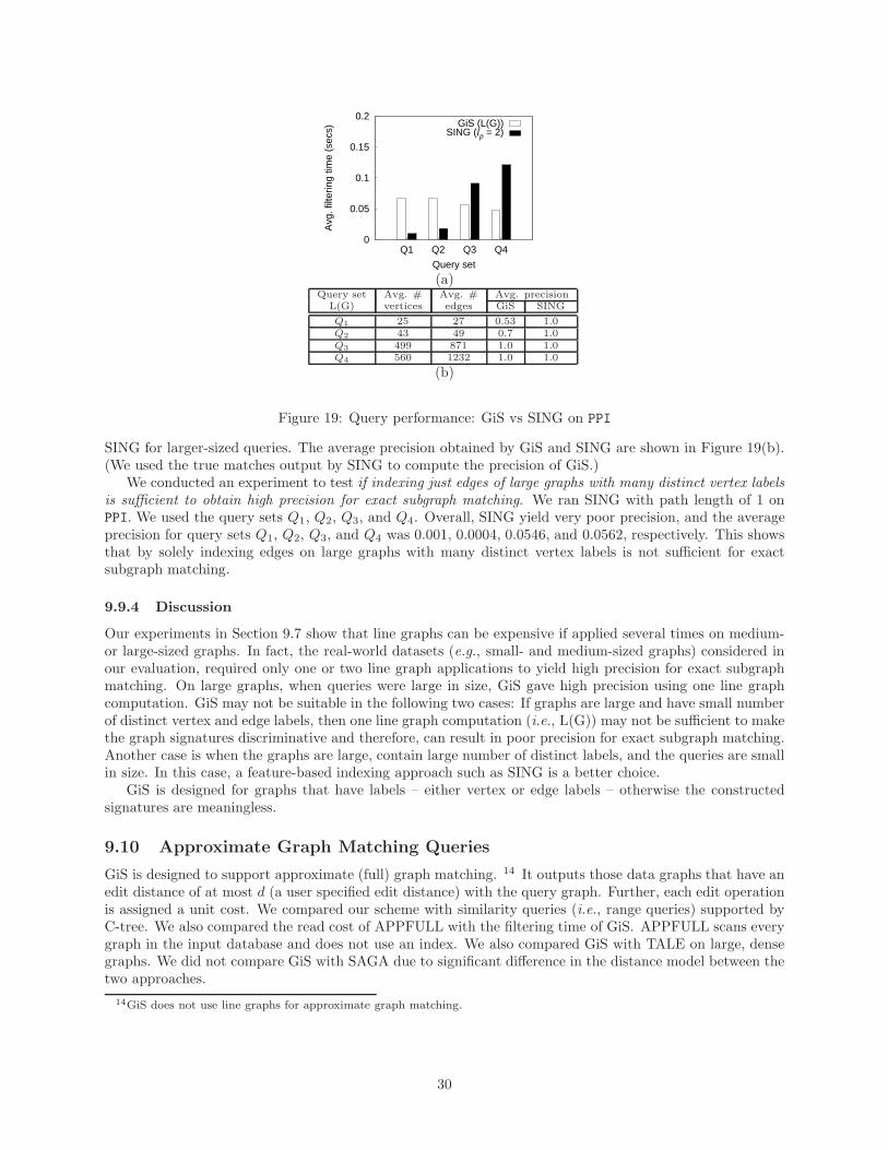
0
0.05
0.1
0.15
0.2
Q1 Q2 Q3 Q4
Avg
. filt
erin
g tim
e (s
ecs)
Query set
GiS (L(G))SING (lp = 2)
(a)Query set Avg. # Avg. # Avg. precision
L(G) vertices edges GiS SING
Q1 25 27 0.53 1.0Q2 43 49 0.7 1.0Q3 499 871 1.0 1.0Q4 560 1232 1.0 1.0
(b)
Figure 19: Query performance: GiS vs SING on PPI
SING for larger-sized queries. The average precision obtained by GiS and SING are shown in Figure 19(b).(We used the true matches output by SING to compute the precision of GiS.)
We conducted an experiment to test if indexing just edges of large graphs with many distinct vertex labelsis sufficient to obtain high precision for exact subgraph matching. We ran SING with path length of 1 onPPI. We used the query sets Q1, Q2, Q3, and Q4. Overall, SING yield very poor precision, and the averageprecision for query sets Q1, Q2, Q3, and Q4 was 0.001, 0.0004, 0.0546, and 0.0562, respectively. This showsthat by solely indexing edges on large graphs with many distinct vertex labels is not sufficient for exactsubgraph matching.
9.9.4 Discussion
Our experiments in Section 9.7 show that line graphs can be expensive if applied several times on medium-or large-sized graphs. In fact, the real-world datasets (e.g., small- and medium-sized graphs) considered inour evaluation, required only one or two line graph applications to yield high precision for exact subgraphmatching. On large graphs, when queries were large in size, GiS gave high precision using one line graphcomputation. GiS may not be suitable in the following two cases: If graphs are large and have small numberof distinct vertex and edge labels, then one line graph computation (i.e., L(G)) may not be sufficient to makethe graph signatures discriminative and therefore, can result in poor precision for exact subgraph matching.Another case is when the graphs are large, contain large number of distinct labels, and the queries are smallin size. In this case, a feature-based indexing approach such as SING is a better choice.
GiS is designed for graphs that have labels – either vertex or edge labels – otherwise the constructedsignatures are meaningless.
9.10 Approximate Graph Matching Queries
GiS is designed to support approximate (full) graph matching. 14 It outputs those data graphs that have anedit distance of at most d (a user specified edit distance) with the query graph. Further, each edit operationis assigned a unit cost. We compared our scheme with similarity queries (i.e., range queries) supported byC-tree. We also compared the read cost of APPFULL with the filtering time of GiS. APPFULL scans everygraph in the input database and does not use an index. We also compared GiS with TALE on large, densegraphs. We did not compare GiS with SAGA due to significant difference in the distance model between thetwo approaches.
14GiS does not use line graphs for approximate graph matching.
30
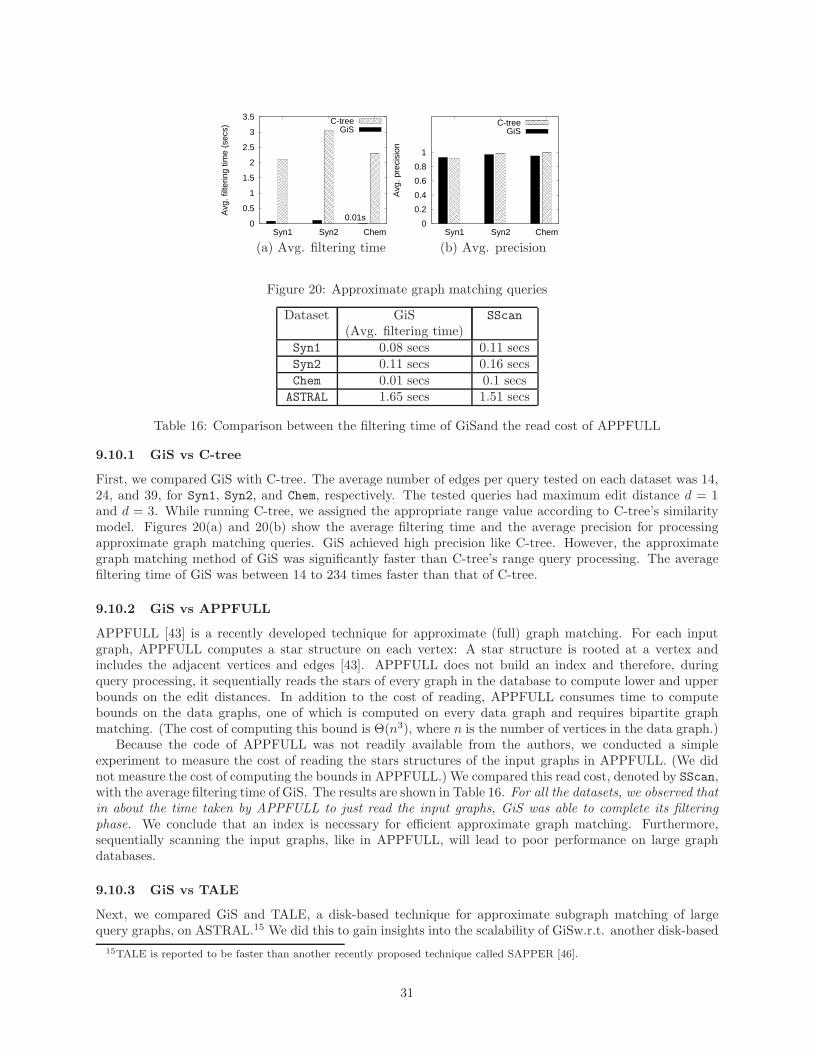
0
0.5
1
1.5
2
2.5
3
3.5
Syn1 Syn2 ChemA
vg. f
ilter
ing
time
(sec
s)0.01s
C-treeGiS
0
0.2
0.4
0.6
0.8
1
Syn1 Syn2 Chem
Avg
. pre
cisi
on
C-treeGiS
(a) Avg. filtering time (b) Avg. precision
Figure 20: Approximate graph matching queries
Dataset GiS SScan
(Avg. filtering time)Syn1 0.08 secs 0.11 secsSyn2 0.11 secs 0.16 secsChem 0.01 secs 0.1 secs
ASTRAL 1.65 secs 1.51 secs
Table 16: Comparison between the filtering time of GiSand the read cost of APPFULL
9.10.1 GiS vs C-tree
First, we compared GiS with C-tree. The average number of edges per query tested on each dataset was 14,24, and 39, for Syn1, Syn2, and Chem, respectively. The tested queries had maximum edit distance d = 1and d = 3. While running C-tree, we assigned the appropriate range value according to C-tree’s similaritymodel. Figures 20(a) and 20(b) show the average filtering time and the average precision for processingapproximate graph matching queries. GiS achieved high precision like C-tree. However, the approximategraph matching method of GiS was significantly faster than C-tree’s range query processing. The averagefiltering time of GiS was between 14 to 234 times faster than that of C-tree.
9.10.2 GiS vs APPFULL
APPFULL [43] is a recently developed technique for approximate (full) graph matching. For each inputgraph, APPFULL computes a star structure on each vertex: A star structure is rooted at a vertex andincludes the adjacent vertices and edges [43]. APPFULL does not build an index and therefore, duringquery processing, it sequentially reads the stars of every graph in the database to compute lower and upperbounds on the edit distances. In addition to the cost of reading, APPFULL consumes time to computebounds on the data graphs, one of which is computed on every data graph and requires bipartite graphmatching. (The cost of computing this bound is Θ(n3), where n is the number of vertices in the data graph.)
Because the code of APPFULL was not readily available from the authors, we conducted a simpleexperiment to measure the cost of reading the stars structures of the input graphs in APPFULL. (We didnot measure the cost of computing the bounds in APPFULL.) We compared this read cost, denoted by SScan,with the average filtering time of GiS. The results are shown in Table 16. For all the datasets, we observed thatin about the time taken by APPFULL to just read the input graphs, GiS was able to complete its filteringphase. We conclude that an index is necessary for efficient approximate graph matching. Furthermore,sequentially scanning the input graphs, like in APPFULL, will lead to poor performance on large graphdatabases.
9.10.3 GiS vs TALE
Next, we compared GiS and TALE, a disk-based technique for approximate subgraph matching of largequery graphs, on ASTRAL.15 We did this to gain insights into the scalability of GiSw.r.t. another disk-based
15TALE is reported to be faster than another recently proposed technique called SAPPER [46].
31
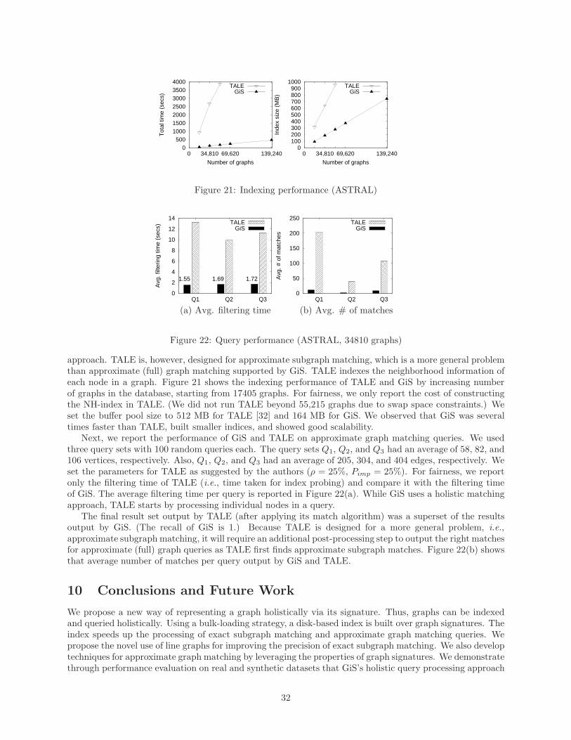
0 500
1000 1500 2000 2500 3000 3500 4000
0 34,810 69,620 139,240T
otal
tim
e (s
ecs)
Number of graphs
TALEGiS
0 100 200 300 400 500 600 700 800 900
1000
0 34,810 69,620 139,240
Inde
x si
ze (
MB
)
Number of graphs
TALEGiS
Figure 21: Indexing performance (ASTRAL)
0
2
4
6
8
10
12
14
Q1 Q2 Q3
Avg
. filt
erin
g tim
e (s
ecs)
1.55 1.69 1.72
TALEGiS
0
50
100
150
200
250
Q1 Q2 Q3
Avg
. # o
f mat
ches
TALEGiS
(a) Avg. filtering time (b) Avg. # of matches
Figure 22: Query performance (ASTRAL, 34810 graphs)
approach. TALE is, however, designed for approximate subgraph matching, which is a more general problemthan approximate (full) graph matching supported by GiS. TALE indexes the neighborhood information ofeach node in a graph. Figure 21 shows the indexing performance of TALE and GiS by increasing numberof graphs in the database, starting from 17405 graphs. For fairness, we only report the cost of constructingthe NH-index in TALE. (We did not run TALE beyond 55,215 graphs due to swap space constraints.) Weset the buffer pool size to 512 MB for TALE [32] and 164 MB for GiS. We observed that GiS was severaltimes faster than TALE, built smaller indices, and showed good scalability.
Next, we report the performance of GiS and TALE on approximate graph matching queries. We usedthree query sets with 100 random queries each. The query sets Q1, Q2, and Q3 had an average of 58, 82, and106 vertices, respectively. Also, Q1, Q2, and Q3 had an average of 205, 304, and 404 edges, respectively. Weset the parameters for TALE as suggested by the authors (ρ = 25%, Pimp = 25%). For fairness, we reportonly the filtering time of TALE (i.e., time taken for index probing) and compare it with the filtering timeof GiS. The average filtering time per query is reported in Figure 22(a). While GiS uses a holistic matchingapproach, TALE starts by processing individual nodes in a query.
The final result set output by TALE (after applying its match algorithm) was a superset of the resultsoutput by GiS. (The recall of GiS is 1.) Because TALE is designed for a more general problem, i.e.,approximate subgraph matching, it will require an additional post-processing step to output the right matchesfor approximate (full) graph queries as TALE first finds approximate subgraph matches. Figure 22(b) showsthat average number of matches per query output by GiS and TALE.
10 Conclusions and Future Work
We propose a new way of representing a graph holistically via its signature. Thus, graphs can be indexedand queried holistically. Using a bulk-loading strategy, a disk-based index is built over graph signatures. Theindex speeds up the processing of exact subgraph matching and approximate graph matching queries. Wepropose the novel use of line graphs for improving the precision of exact subgraph matching. We also developtechniques for approximate graph matching by leveraging the properties of graph signatures. We demonstratethrough performance evaluation on real and synthetic datasets that GiS’s holistic query processing approach
32

provides a scalable and efficient disk-based solution for indexing and querying a large database of graphs.In the design of GiS, we did not focus on speeding up the verification phase. While GiS could quickly
filter through a database of large graphs (e.g., protein interaction networks), the verification phase of exactsubgraph matching became the bottleneck. To overcome this, we would like to annotate a graph signaturewith vertex and edge information in the original graph so that we can speed up the verification phase byfocusing on smaller portions of a candidate data graph. We would also like to extend the implementation ofGiS to support the insertion and deletion of graph signatures from the graph signature index.
Acknowledgments
We are grateful to the authors of C-tree, FG-index, SING, and TALE for their code and assistance. Thiswork was supported in part by the National Science Foundation under Grant No. 1115871.
References
[1] M. A. Bayir, T. D. Guney, and T. Can. Integration of topological measures for eliminating non-specificinteractions in protein interaction networks. Discrete Appl. Math., 157:2416–2424, 2009.
[2] A. Broder. On the resemblance and containment of documents. In Proc. of the Compression andComplexity of Sequences 1997, 1997.
[3] N. Bruno, N. Koudas, and D. Srivastava. Holistic twig joins: Optimal XML pattern matching. In Proc.of the 2002 SIGMOD Conference, Wisconsin Madison, WI, 2002.
[4] C. Calude, G. Paun, G. Rozenberg, and A. Salomaa. Multiset Processing: Mathematical, ComputerScience, and Molecular Computing Points of View. Springer, 2001.
[5] J. Cheng, Y. Ke, A. Fu, and J. Yu. Fast graph query processing with a low-cost index. The VLDBJournal, pages 1–19, 2010.
[6] J. Cheng, Y. Ke, W. Ng, and A. Lu. FG-index: Towards verification-free query processing on graphdatabases. In Proc. of the 2007 SIGMOD Conference, pages 857–872, Beijing, China, 2007.
[7] J. Cheng, Y. Ye, and W. Ng. Efficient Query Processing on Graph Databases. ACM Transactions onDatabase Systems, 34(1):1–48, 2009.
[8] N. V. Dokholyan, L. Li, F. Ding, and E. I. Shakhnovich. Topological Determinants of Protein Folding.Proceedings of the National Academy of Sciences, 99(13):8637–8641, 2002.
[9] M. R. Garey and D. S. Johnson. Computers and Intractability : A Guide to the Theory of NP-Completeness . Freeman, 1979.
[10] R. Giugno and D. Shasha. GraphGrep: A Fast and Universal Method for Querying Graphs. Intl. Conf.on Pattern Recognition, 2002.
[11] A. Golovin and K. Henrick. Chemical Substructure Search in SQL. Jour. of Chem. Info. and Modeling,49(1):22–27, 2009.
[12] A. Guttman. R-trees: A dynamic index structure for spatial searching. In Proc. of the 1984 SIGMODConference, pages 47–57, June 1984.
[13] W.-S. Han, J. Lee, M.-D. Pham, and J. X. Yu. igraph: a framework for comparisons of disk-based graphindexing techniques. Proc. VLDB Endow., 3:449–459, September 2010.
[14] R. Haralick and G. Elliott. Increasing tree search efficiency for constraint satisfaction problems. ArtificialIntelligence, 14(3):263–313, Oct 1980.
33

[15] H. He and A. K. Singh. Closure-tree: An index structure for graph queries. In Proc. of the 22th ICDEConference, pages 38–49, 2006.
[16] J. Hellerstein and A. Pfeffer. The RD-Tree: An Index Structure for Sets. Technical Report UW-CS-TR-1252, Univ. of Wisconsin Madison, 1994.
[17] J. Hu, X. Shen, Y. Shao, C. Bystroff, and M. J. Zaki. Mining Protein Contact Maps. In BIOKDD02:Workshop on Data Mining in Bioinformatics, pages 3–10, 2002.
[18] H. Jiang, H. Wang, P. S. Yu, and S. Zhou. GString: A novel approach for efficient search in graphdatabases. In Proc. of the 23th ICDE Conference, pages 566–575, 2007.
[19] M. Kuramochi and G. Karypis. An Efficient Algorithm for Discovering Frequent Subgraphs. IEEETransactions on Knowledge and Data Engineering, 16(9):1038–1051, 2004.
[20] B. T. Messmer and H. Bunke. Efficient subgraph isomorphism detection: A decomposition approach.IEEE Transactions on Knowledge and Data Engineering, 12(2):307–323, 2000.
[21] J. Nacher, T. Yamada, S. Goto, M. Kanehisa, and T. Akutsu. Two complementary representations ofa scale-free network. Physica A, 349:349–363, 2005.
[22] R. D. Natale, A. Ferro, R. Giugno, M. Mongiov, A. Pulvirenti, and D. Shasha. SING: Subgraph Searchin Non-Homogeneous Graphs. BMC Bioinformatics, 11(1):96–96, Feb 2010.
[23] M. Neuhaus and H. Bunke. Bridging the Gap Between Graph Edit Distance and Kernel Machines.World Scientific Publishing, 2007.
[24] D. Pal and P. R. Rao. A tool for fast indexing and querying of graphs. In Proceedings of the 20thinternational conference companion on World wide web, pages 241–244, 2011.
[25] J. B. Pereira-Leal, A. J. Enright, and C. A. Ouzounis. Detection of functional modules from proteininteraction networks. Proteins: Structure, Function, and Bioinformatics, 54(1):49–57, 2004.
[26] M. O. Rabin. Fingerprinting by Random Polynomials. Technical Report TR 15-81, Harvard University,Cambridge, MA 02138, 1981.
[27] P. Rao and B. Moon. Locating XML Documents in a Peer-to-Peer Network using Distributed HashTables. IEEE Transactions on Knowledge and Data Engineering, 21(12):1737–1752, December 2009.
[28] K. Riesen and H. Bunke. Approximate graph edit distance computation by means of bipartite graphmatching. Journal of Image and Vision Computing, 27(7):950–959, June 2009.
[29] H. Shang, X. Lin, Y. Zhang, J. X. Yu, and W. Wang. Connected substructure similarity search. InProc. of the 2010 SIGMOD Conference, pages 903–914, Indianapolis, 2010.
[30] H. Shang, Y. Zhang, X. Lin, and J. X. Yu. Taming Verification Hardness: An Efficient Algorithm forTesting Subgraph Isomorphism. In Proc. of the 34st VLDB Conference, pages 364–375, 2008.
[31] Y. Tian, R. C. McEachin, C. Santos, D. J. States, and J. M. Patel. SAGA: A Subgraph Matching Toolfor Biological Graphs. Bioinformatics Journal, 23(2):232–239, 2007.
[32] Y. Tian and J. M. Patel. TALE: A Tool for Approximate Large Graph Matching. In Proc. of the 24thICDE Conference, pages 963–972, Cancun, 2008.
[33] D. Ucar, S. Parthasarathy, S. Asur, and C. Wang. Effective pre-processing strategies for functionalclustering of a protein-protein interactions network. In 5th IEEE Symposium on Bioinformatics andBioengineering, pages 129–136, 2005.
[34] J. R. Ullmann. An algorithm for subgraph isomorphism. Journal of ACM, 23(1):31–42, 1976.
[35] A. van Rooij and H. S. Wilf. The interchange graph of a finite graph. Acta Mathematica Hungarica,16(3-4):263–269, 1965.
34

[36] J. T. Wang, K. Zhang, and G.-W. Chirn. Algorithms for approximate graph matching. InformationSciences - Informatics and Computer Science, 82(1-2):45–74, 1995.
[37] P. Willett, J. Barnard, and G. Downs. Chemical Similarity Searching. Jour. of Chem. Info. andComputer Sciences, 38(6):983–996, 1998.
[38] D. W. Williams, J. Huan, and W. Wang. Graph database indexing using structured graph decomposi-tion. In Proc. of the 23th ICDE Conference, pages 976–985, Istanbul, 2007.
[39] R. J. Wilson. Introduction to Graph Theory. Longman, 1999.
[40] X. Yan, P. Yu, and J. Han. Graph indexing: A frequent structure based approach. In Proc. of the 2004SIGMOD Conference, 2004.
[41] X. Yan, P. S. Yu, and J. Han. Substructure similarity search in graph databases. In Proc. of the 2005SIGMOD Conference, pages 766–777, Baltimore, 2005.
[42] X. Yan, F. Zhu, J. Han, and P. S. Yu. Searching Substructures with Superimposed Distance. In Proc.of the 22th ICDE Conference, pages 88–99, Atlanta, 2006.
[43] Z. Zeng, A. K. Tung, J. Wang, J. Feng, and L. Zhou. Comparing Stars: On Approximating Graph EditDistance. In Proc. of the 35st VLDB Conference, Lyon, France, 2009.
[44] S. Zhang, M. Hu, and J. Yang. TreePi: A Novel Graph Indexing Method. In Proc. of the 23th ICDEConference, pages 966–975, Istanbul, 2007.
[45] S. Zhang, S. Li, and J. Yang. Gaddi: distance index based subgraph matching in biological networks.In Proceedings of the 12th International Conference on Extending Database Technology: Advances inDatabase Technology, EDBT ’09, pages 192–203, Saint Petersburg, Russia, 2009.
[46] S. Zhang, J. Yang, and W. Jin. SAPPER: subgraph indexing and approximate matching in large graphs.In Proc. of the 36th VLDB Conference, pages 903–914, Singapore, 2010.
[47] P. Zhao, J. X. Yu, and P. S. Yu. Graph indexing: tree + delta >= graph. In Proc. of the 33rd VLDBConference, pages 938–949, 2007.
[48] L. Zou, L. Chen, J. X. Yu, and Y. Lu. A Novel Spectral Coding in a Large Graph Database. In Proc.of the 11th Intl. Conference on Extending Database Technology, 2008.
Appendix A
Theorem 1
Given a data graph G and a query graph Q, if Q is a subgraph of G, then sig(Q) ⊆ sig(G).Proof. By definition, if Q is a subgraph of G, then every edge of Q appears in G. While applying
Algorithm 1 on Q, all the ordered-label pairs in Q were also considered during the signature construction forG. Thus each hash value p that was added to the signature sig(Q) (Line 5 in Algorithm 1), was also addedto the signature sig(G). Therefore, all the hash values in sig(Q) are present in sig(G), and hence sig(Q) ⊆sig(G).
Theorem 2
Suppose G and Q denote a data graph and a query graph, and their line graphs L(G) and L(Q) have at leasttwo vertices each. If Q is a subgraph of G, then sig(L(Q)) ⊆ sig(L(G)).
Proof.We first show that if Q is a subgraph of G, then L(Q) is a subgraph of L(G). Let us focus on the vertex
set of L(Q) and L(G). Without loss of generality, consider an edge (vqi, vqj) in Q. Because Q is a subgraphof G, there exists an edge with labels L(vqi) and L(vqj) in G. Let (vgk, vgl) denote such an edge in G. Edge
35

(vqi, vqj) has a vertex in L(Q) according to the definition of a line graph. Similarly, (vgk, vgl) has a vertexin L(G). Further their vertex labels are the same because lex(l(vqi), l(vqj)) = lex(l(vgk), l(vgl)).
The above condition is true for every edge in Q. Therefore the vertex set of L(Q) is a subset of the vertexset of L(G).
Let us focus on the edge set of L(Q) and L(G). Without loss of generality, suppose edges (vqi, vqj) and(vqi, vqk) are adjacent in Q. Since Q is a subgraph of G, there exists a corresponding pair of edges in G say(vgl, vgm) and (vgl, vgn) that are adjacent. Then l(vqi) = l(vgl), l(vqj) = l(vgm), and l(vqk) = l(vgn). In L(Q),there exists an edge (lex(vqi, vqj), lex(vqi, vqk)). In L(G), there exists an edge (lex(vgl, vgm), lex(vgl, vgn)).This edge in L(G) has the same vertex labels as that of the edge in L(G). (This is because l(vqi) = l(vgl),l(vqj) = l(vgm), and l(vqk) = l(vgn).) This is true for every edge in L(Q), and therefore the edge set of L(Q)is a subset of the edge set of L(G).
Hence, it is proved that L(Q) is a subgraph of L(G). Now we can apply the ideas in Theorem 1 to showthat sig(L(Q)) ⊆ sig(L(G)).
Theorem 3
Suppose G and Q denote a data graph and a query graph. Let n (≥ 0) denote the number of line graphcomputations on the data and query graphs. Suppose Ln(G) and Ln(Q) have at least two vertices. If Q is asubgraph of G, then sig(Ln(Q)) ⊆ sig(Ln(G)).
Proof.We prove the theorem by Induction on the number of line graph computations. Let P (k) denote the
proposition that if Q is a subgraph of G, then sig(Lk(Q)) ⊆ sig(Lk(G)). Note that 1 ≤ k ≤ n.(1) Basis of Induction: P (0) is true. If Q is a subgraph of G, then sig(L0(Q)) ⊆ sig(L0(G). This was
proved in Theorem 1.(2) Induction Hypothesis: Assume that P (i) is true for 1 ≤ i ≤ k. We will show that P (k + 1) is true.
Now Lk+1(Q) = L(Lk(Q)) and Lk+1(G) = L(Lk(G)). If Lk(Q) is a subgraph of Lk(G), then Lk+1(Q) isa subgraph of Lk+1(G) (by Theorem 2). By induction hypothesis, if Q is a subgraph of G, then Lk(Q) isa subgraph of Lk(G). By transitivity, if Q is a subgraph of G, then Lk+1(Q) is a subgraph of Lk+1(G).Therefore, sig(Lk+1(Q)) ⊆ sig(Lk+1(G)). Thus P (k + 1) is true.
Theorem 4
Given a query graph Q and a data graph G, let d (≥ 1) denote a user specified maximum edit distance. Letm1, ...,mn denote the degrees of n vertices in Q ranked in descending order. Let | · | denote the cardinalityof a signature. If Q has an approximate graph match with G such that ged(Q,G) ≤ d, then
|sig(Q)− sig(G)| ≤ maxInfd,
where maxInfd = (∑min{d,n}
i=1 mi) +max{0, d− n}.Proof.Suppose d ≤ n. There are many different edit paths of cost d that could transform G to Q. Among
these, the one that maximizes the total influence is the edit path with d vertex relabels. This is becauseInf(vR) ≥ 1. We denote this maximum total influence for edit distance d by maxInfd. By computing|sig(Q)− sig(G)|, we are computing the count of those items that are in Q but do not have a counterpartin G. The value maxInfd provides an upper bound for this count. As we do not know which vertices are tobe relabeled when the query is posed, we compute the value of maxInfd by summing the d highest vertexdegrees of Q, i.e.,
∑di=1 mi.
Suppose d > n. Then at most n relabels can be present as there are only n vertices in Q. The remainingd − n edit distance should be contributed by the remaining edit operations. Each of these edit operationshas an influence of 1. Therefore, an additional term max{0, d− n} is needed.
36