Using GIS to Optimize Gathering Line Operations and Maintenance

– A Risk Based Approach

W. Kent Muhlbauer

WKM Consultancy

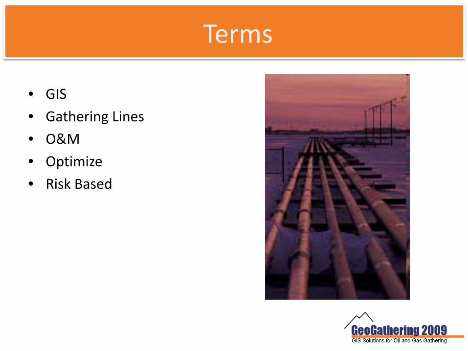
Terms

• GIS

• Gathering Lines

• O&M

• Optimize

• Risk Based

Gathering PL:  One of Several Types of PL

… sometimes with unique designs

… and special requirements

… in interesting areas

… and in challenging areas

Definitions (for presentation)

• GIS = computer tools to use and manage data

• Gathering Line = a type of PL

• O&M = activities of running a PL

• Optimize = to make better

• Risk Based– Risk = PoF x CoF

– Risk‐based = using an understanding of risk

Key Message

Understanding Risk = Better Decision‐Making

Unprecedented Opportunities to Understand Risk

Data Drives the Process

“If you don’t have a number, you don’t have a fact; you have an opinion”

IM Rule Data (Liquids)

• HCA info

• Results from previous testing inspection

• Leak history

• Corrosion or condition data

• CP history

• Soil corrosivity

• Type and quality of coating

• Age of pipe

• Product characteristics

• Pipe wall

• Pipe diameter

• Subsidence 

• All ground movement potential

• Security of thru‐put

• Time since last inspection

• Defect growth rates

• Stress levels

• Leak detection

• Physical support

IM Rule Data (Gas) Data Elements for Prescriptive IMP

Attribute Data– Pipe wall

– Pipe OD

– Seam type

– Manufacturer

– Date of manufacture

– Material properties

– Equipment properties

Inspection– Pressure tests

– In‐line inspections

– Geometry inspections

– Bell hole inspections

– CP & close‐interval surveys

– Coating condition and DCVG

– surveys

– Audits & reviews

ASME B31.8S Section 4

IM Rule Data (Gas) Data Elements for Prescriptive IMP, Cont’d

Construction– Year installed– Bending method– Joining method and– inspection– Depth of cover– Crossings, casings– Pressure test– Coating type– Field coating method– Soil and backfill– Cathodic protection– Inspection reports

ASME B31.8S Section 4

Gas IM RuleData Elements for Prescriptive IMP

Considerations:

• Data must support risk assessment

• Data age and accuracy

• Missing data is not justification to exclude a threat from the IMP

• Common reference system needed – GIS and geospatial referencing a practical necessity for all but simplest systems

• Appendix A gives additional data needs on a threat specific basis

ASME B31.8S Section 4

Dealing with Uncertainty

Error 1:  Call it ‘good’ when its really ‘bad’

Error 2:  Call it ‘bad’ when its really ‘good’

Use of Data

• Not everything that matters can be counted;

• Not everything that can be counted matters

‐Albert Einstein

Data Collection; Maintenance; Sectioning

swamp

Metropolis

A B C

Risk Analysis:  Turning Data into Information 

• Risk = Probability x Consequences

• Probability = Degree of Belief• Risk Mitigation via Integrity Mgmt in HCA

Threat Categories• ASME B31.8 Supplement considers 3 categories of threat:

– Time Dependent – May worsen over time; require periodic reassessment

– Time Stable – Does not worsen over time; one‐time assessment is sufficient (unless conditions of operation change)

– Time Independent – Occurs randomly; best addressed by prevention

Time Dependent Threats

• External corrosion

• Internal corrosion

• Stress‐corrosion cracking (SCC)

• Fatigue

Time Stable Threats (resistance)

• Manufacturing‐related flaws in

– Pipe body

– Pipe seam

• Welding / Fabrication‐caused flaws in

– Girth welds

– Fabrication welds

– Wrinkled / buckled bend

– Threads / couplings

• Defects present in equipment

– Gaskets, O‐rings

– Control / relief devices

– Seals, packing

– Other equipment

Time Independent (Random) Threats

• Third‐party/Mechanical damage– Immediate failure

– Delayed failure (previously damaged)

– Vandalism

• Incorrect operations

• Weather related– Cold weather

– Lightning

– Heavy rain, flood

– Earth movement

Failure Mechanisms

Corrosion; fatigue

3rd party, earth movements, human 

error

Failures

Time

Hawthorne Effect

“Anything that is studied, improves.”

Better Estimates:  Absolute Risk Values

Frequency of consequence– Temporally

– Spatially•Incidents per mile-year

•fatalities per mile-year

•dollars per km-decade

conseq prob

Better Modeling:  PoF Triad

• Exposure:  frequency or intensity of failure mechanism(s) reaching the pipe 

when no mitigation applied

• Mitigation measure:  reduces frequency or intensity of the exposure 

reaching the pipe; keeps mechanism off the pipe

• Resistance:  ability to resist failure given presence of exposure/threat

attack > defense > survival

Potential for Damage vs Failure

• Probability of Damage (PoD) = f (exposure, mitigation)

• Probability of Failure (PoF) = f (PoD, resistance)

Exposure     

PoD

Mitigation

PoF

Resistance

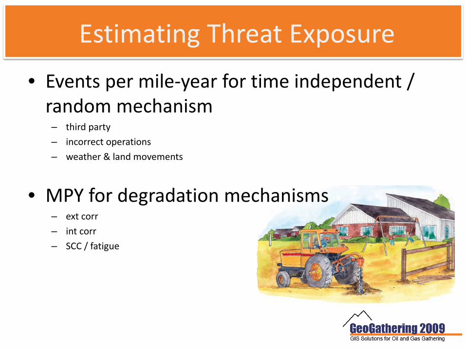
Estimating Threat Exposure

• Events per mile‐year for time independent / random mechanism

– third party

– incorrect operations

– weather & land movements

• MPY for degradation mechanisms– ext corr

– int corr

– SCC / fatigue

Rates:  Failures, Exposures, Events, etc

Failures/yr Years to Fail Approximate Rule Thumb 1,000,000 0.000001 Continuous failures

100,000 0.00001 fails ~10 times per hour

10,000 0.0001 fails ~1 times per hour 1,000 0.001 fails ~3 times per day

100 0.01 fails ~2 times per week 10 0.1 fails ~1 times per month 1 1 fails ~1 times per year

0.1 10 fails ~1 per 10 years 0.01 100 fails ~1 per 100 years

0.001 1,000 fails ~1 per 1000 years 0.0001 10,000 fails ~1 per 10,000 years

0.00001 100,000 fails ~1 per 100,000 years 0.000001 1,000,000 One in a million chance of failure

0.0000000001 1,000,000,000 Effectively, it never fails

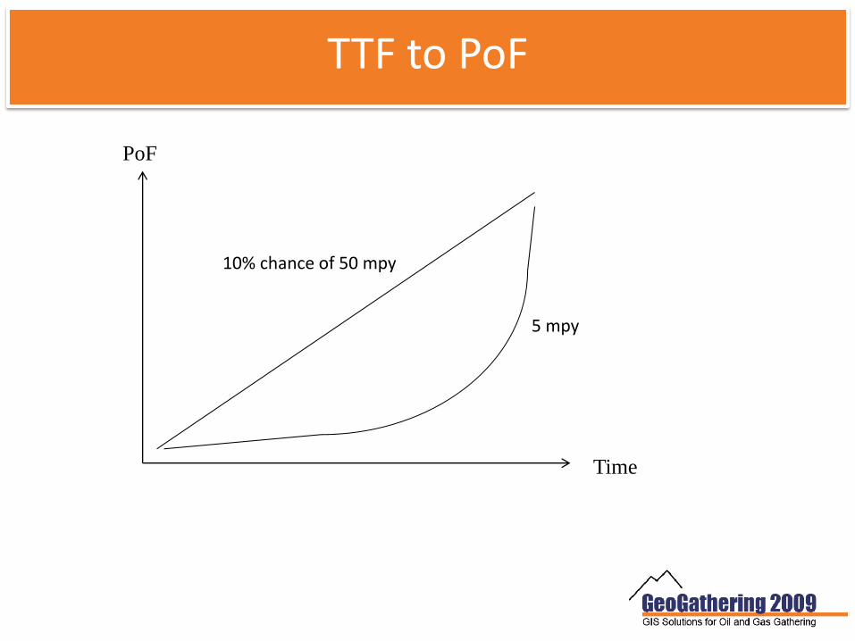
Time Dependent Mechanisms

PoF time‐dep = f (TTF)  

whereTTF  = “time to failure”

TTF = (available pipe wall) / [(unmitigated mpy) x (1 – mitigation effectiveness)]

Time

PoF

TTF to PoF

5 mpy

10% chance of 50 mpy

PoF:  TTF & TTF99

time

PoF PoF=100%

PoF=1%

TTF99

Measuring MitigationStrong, single measure or  Accumulation of lesser measures

Mitigation % = 1‐[(1‐mit1) x (1‐mit2) x (1‐mit3)…]

In words:  mitigation %  = 1 ‐ (remaining threat)

remaining threat = (remnant from mit1) AND (remnant from mit2) AND (remnant from mit3) …

What is cumulative mitigation benefit from 3 measures that independently produce effectiveness of 60%, 60%, and 50%?

92%

Exposure Mitigation Reduction freq damage prob damageevents/mi-yr events/mi-yr Prob/mi-yr

10 90.0% 10 1 63.2%10 99.0% 100 0.1 9.52%10 99.9% 1000 0.01 1.00%

Best Estimate of Pipe Wall Today

Press Test 1

Press Test 2

Bell Hole 1

Bell Hole 2

ILI 1

ILI 2

NOP

Best Est Today

Final PoF

PoF overall = PoFthdptyOR PoFcorr ext OR PoFcorr intOR PoFincopsOR PoFgeohazard

PoS = 1‐ PoF

PoF overall = 1‐[(1‐PoFthdpty) x (1‐PoFcorr ext) x (1‐PoFcorr int) x (1‐PoFincops) x 

(1‐PoFgeohazard)]

Understanding Consequence of Failure

• Risk = (PoF)∙(Consequence)

• Consequence of Failure– Leak vs rupture

– Estimate of hazard area

– Estimate of damages (property, people, etc) 

Initiating Event

Hazard Zones

Hazard Zone

Spill pathPL

HCA

PIR Calculations

TTO13 & TTO14

Receptor Characterization

•fatalities•injuries•occupancy•shielding•escape•prop damage•waterways•ground water•wetlands•T&E wildlife•preserves•historical sites

PL

Hwy

Hwy

Monetized Risk:  Expected LossSurrogate for ‘risk’ and ‘financial exposure’

• Benefits– Common denominator allows unlimited comparisons 

– Defines the magnitude of the problem– Implies appropriate reaction

• Difficulties– Some consequences difficult to monetize– Annual (averages) vs Extremes

Damage State Estimates

Hazard Zone injury rate fatality rate

environ damage rate

service interruption rate

<100' 80% 8% 50% 100% 100'-50% PIR 50% 5% 30% 90% 50% -100% PIR 20% 2% 10% 80%

•Create Zones Based on Threshold Distances•Estimate Damage States (or PoD) for Each Zone

Sample EL Calculations

unit cost unit cost unit cost

$100,000

$3,500,000 $ 50,000 Expected

Loss

Hole Size

Ignition Scenario

Maximum Distance (ft)

Probability of

Maximum Distance

Hazard Zone Group

# people

Human injury costs

Human fatality costs

# environ

units

Environ Damage Costs

Probability weighted

dollars per failure

immediate 400 4.8% 100'-50% PIR 5 $ 3,600 $ 12,600 1 $ 720 $ 16,920 delayed 1500 1.6% 50% -100% PIR 10 $ 960 $ 3,360 1 $ 80 $ 4,400 rupture no ignition 300 1.6% 100'-50% PIR 5 $ 1,200 $ 4,200 1 $ 240 $ 5,640 immediate 300 1.8% 100'-50% PIR 5 $ 1,350 $ 4,725 1 $ 270 $ 6,345 delayed 600 1.8% 100'-50% PIR 5 $ 1,350 $ 4,725 1 $ 270 $ 6,345 medium no ignition 100 8.4% 100'-50% PIR 5 $ 6,300 $ 22,050 1 $ 1,260 $ 29,610 immediate 50 8.0% <100' 1 $ 1,920 $ 6,720 0.5 $ 1,000 $ 9,640 delayed 80 8.0% <100' 1 $ 1,920 $ 6,720 0.5 $ 1,000 $ 9,640 small no ignition 30 64.0% <100' 1 $15,360 $ 53,760 0.5 $ 8,000 $ 77,120

100.0% Total expected loss per failure at this location $165,660

Final EL Value

At a specific location along a pipeline:Expected Loss

Failure Rate (failures per mile-year)

Probability of Hazard Zone1,2

Probability weighted dollars2,3

Probability weighted dollars

per mile-year 4.80% $16,920 $0.81 1.60% $4,400 $0.07 1.60% $5,640 $0.09 1.80% $6,345 $0.11 1.80% $6,345 $0.11 8.40% $29,610 $2.49 8.00% $9,640 $0.77 8.00% $9,640 $0.77

0.001

64.00% $77,120 $49.36 100.00% $165,660 $54.59

Table Notes1. after a failure has occurred2. from Table 2 above, per event3. (damage rate) x (value of receptors in hazard zone), per event

Expected Losses Vary Along PL

swamp

$

$

Hazard zones

Expected Losses

…identify model and pipeline specifications (e.g., product)

…determine the interval spacing or read point

locations from a stored file of X,Y points

Step 1: Determine On-Line Sampling Interval

Z1Z2

Z3

…determine the # of zones and reach

defining each zone

Step 2: Establish Hazard Zones

Z1Z2

Z3

…count the number of

houses within each zone

Step 3: Determine Number of Houses in Each Zone (Point Features)

Z1Z2

Z3

…calculate the length of

waterway within each zone

Step 4: Determine Length of Waterways in Each Zone (Line Features)

Z1Z2

Z3

HPA

ESA

Z1Z2

Z3

…calculate the area of each HCA within each zone

Step 5: Determine Area of HCAs in Each Zone (Polygon Features)

Z1Z2

Z3

Z1Z2

Z3…convert the

counts, lengths, and areas of impacted

features into estimated impacts

within each hazard zone

Summarize Impacted Receptors (Data Table)

Hazard Zones & Consequence Estimates

…delineate impact area to

identify window center (e.g. oil

spill)

Z2 Z3Z1

calculate Expected

Loss

The Sliding Impact Area based on—

• Product specifications• Spill quantity• Terrain configuration• Infiltration, evaporation

and Pooling

Expected Loss Calcs (Probability * Impacted Feature Valuation)

Each row represents one pipeline release location

Expected Loss is a function of each Zone’s Probability of occurring and the Zone’s Potential LossExpected Loss = (Z1_Prob * Z1_PLoss) + (Z2_Prob * Z2_PLoss) + (Z3_Prob * Z3_PLoss)

EL20 = (.88 * 101660) + (.07 * 15812) + (.07 * 28609) = $146,081 …considerable risk exposure at this location

One injuryOne property damaged

Two injuriesThree properties damaged

Three injuriesTwelve properties damaged

Visualization of Risks

•EL for entire PL•EL changes along PL•PoF at all points•Compiled PoF•“Hot spots” for each failure mechanism•TTF --> Re-assess interval

$

$$$

If you put tomfoolery into a computer, nothing comes out of it but tomfoolery. But this tomfoolery, having passed through a very expensive machine, is somehow ennobled and no‐one dares criticize it.

‐ Pierre Gallois

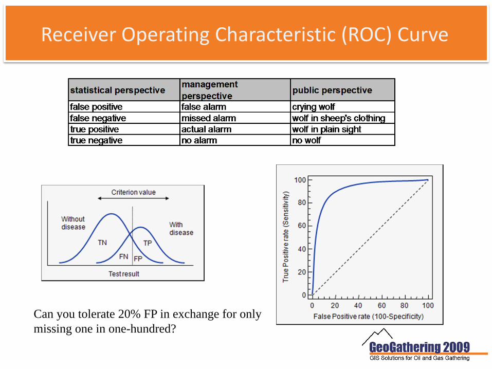
Receiver Operating Characteristic (ROC) Curve

Can you tolerate 20% FP in exchange for only missing one in one-hundred?

Optimizing O&M

Resource Allocation Modeling

Responding to Changes Along ROWRisk‐based thinking to avoid inefficient, one‐size‐fits‐all solutions

Example:  Increased CoF potential

– Change CoF• Product, pressure, ignition, containment, response

– Change PoF• Design factors• Respond to threat(s)

– Increase patrol– Protective slab– Surveys:  coating, CP– Training– Geotech study

Reported Mitigation Benefits

Mitigation Impact on risk

Increase soil cover56% reduction in mechanical damage when soil cover increased from 1.0 to 1.5 m

Deeper burial25% reduction in impact failure frequency for burial at 1.5 m; 50% reduction for 2m; 99% for 3m

Increased wall thickness90% reduction in impact frequency for >11.9-mm wall or >9.1-mm wall with 0.3 safety factor

Concrete slab Same effect as pipe wall thickness increaseConcrete slab Reduces risk of mechanical damage to “negligible” Underground tape marker 60% reduction in mechanical damageAdditional signage 40% reduction in mechanical damageIncreased one-call awareness and response 50% reduction in mechanical damageIncreased ROW patrol 30% reduction in mechanical damage

Increased ROW patrol30% heavy equipment-related damages; 20% ranch/farm activities; 10% homeowner activities

Improved ROW, signage, public education 5–15% reduction in third-party damages

Risk Management Options

Resource Allocation Choice Cost Impact Risk Impact

Increase Public Education +  $4000 ‐ 0.8%

Perform Close Interval Survey +  $11000 ‐ 2.6%

Reduce Air Patrol ‐ $7600 + 1.1%

Perform Hydrostatic Test + $67000 ‐ 8.2%

Action Triggers / Strategies

Risk

Frequency

When to take actionProportional level of action

What is “Safe Enough”?• Many risk levels are considered insignificant or tolerable

– Regulatory precedents

• ALARP 

• land use/facility siting

• Environmental clean up criteria

• EIS, EA

– Industry precedents

• Reliability Based Design

• Limit state

– Often measured in terms of fatalities

• Philosophical challenges placing this in IMP context– ‘acceptable risk’ argument is not explicitly recognized in IMP

– very low risk levels can be shown in many covered segments, especially when short

Acceptable Risk

Canadian Risk‐Based Land Uses

10‐4

10‐5

10‐6

CSChE Risk Assessment – Recommended Practices, MIACC risk acceptability

Nessim et al.  Target Reliability Levels for Design and Assessment ofOnshore Natural Gas Pipelines.  International Pipeline Conference, Calgary, Alberta, 2004 

Failurelocation

AffectedArea

Number of people affected = A x P x ρAffected area ‐ proportional to pd2

Population density

Ignition probability ‐ proportional to d

Expected number of people affected α ρpd3

Reliability Based Design

Safety risk

New Possibilities:  Reliability Targets

PRCI work– Acceptable risk as implied by current regs & stds

– Based on probability of fatality 

– Considers both individual and societal risk criteria

– Annex in CSA Z662; considered for ASME B31.8

– Tolerable PoF:  5E‐5 failures per km‐yr in Class 3

(Nessim, et al, IPC 2002, 2004, 2006)

Unprecedented opportunities to understand risk issues

New Tools & Techniques 

New ways of thinking emerging

New Possibilities: Optimizing Decisions

Range of Opportunities

From

Tweaking existing O&M programs and design protocols

To

Establishing corporate/regional/national acceptable risk levels

He who shoots at nothing, hits nothing

Chinese proverb