global and finite termination of a two-phase …

GLOBAL AND FINITE TERMINATION OF A TWO-PHASEAUGMENTED LAGRANGIAN FILTER METHOD FOR

GENERAL QUADRATIC PROGRAMS∗

MICHAEL P. FRIEDLANDER† AND SVEN LEYFFER‡

Abstract. We present a two-phase algorithm for solving large-scale quadratic programs (QPs).In the first phase, gradient-projection iterations approximately minimize a bound-constrained aug-mented Lagrangian function and provide an estimate of the optimal active set. In the second phase,an equality-constrained QP defined by the current active set is approximately minimized in order togenerate a second-order search direction. A filter determines the required accuracy of the subproblemsolutions and provides an acceptance criterion for the search directions. The resulting algorithm isglobally and finitely convergent. The algorithm is suitable for large-scale problems with many degreesof freedom, and provides an alternative to interior-point methods when iterative methods must beused to solve the underlying linear systems. Numerical experiments on a subset of the CUTEr QPtest problems demonstrate the effectiveness of the approach.

Key words. Large-scale optimization, quadratic programming, gradient-projection, active-setmethods, filter methods, augmented Lagrangian.

AMS subject classifications. 65K05, 90C06, 90C20, 90C26, 90C52

1. Introduction. Quadratic programs (QPs) play a fundamental role in opti-mization. They are useful across a rich class of applications, such as the simulationof rigid multibody dynamics [2, 50], optimal control [7, 32, 53], and financial-portfoliooptimization [15,54]. They also arise as a sequence of subproblems within algorithmsfor solving more general nonlinear optimization problems. Of particular interest forus are sequential quadratic programming (SQP) methods, which have proved to be areliable approach for general problems (for a recent survey, see Gould and Toint [47]).Our purpose is to develop a QP algorithm that may be used effectively within an SQPframework for solving large-scale nonlinear problems.

Compared to interior-point methods for QPs, active-set methods are especiallyeffective as subproblem solvers within the SQP framework because they can exploitincreasingly good starting points in order to reduce the number of iterations requiredfor convergence. Inertia-controlling active-set strategies (see, e.g., [33,43]) are robustin practice, but their overall efficiency is limited by the number of active-set changesthat can be made at each iteration (typically, a single index changes at each iteration).The combinatorial nature of such an approach severely limits its effectiveness on trulylarge-scale, nonconvex problems that may have many degrees of freedom. However,the robustness and warm-start capability of active-set approaches motivate us topropose a method that is capable of extremely large changes to the active set at eachiteration and yet continues to be finitely convergent.

Interior-point methods are often preferred over active-set approaches because theyhave proved effective for large problems and because they have strong theoretical con-

∗Preprint ANL/MCS-P1370-0906 and UBC Department of Computer Science Tech. Rep. TR-2007-16. To appear in SIAM J. Sci. Comp., Revised August 30, 2007†Department of Computer Science, University of British Columbia, Vancouver, BC V6T 1Z4,

Canada, [email protected]. The research of this author was supported in part by a Discovery Grantfrom the National Science and Engineering Research Council of Canada.‡Mathematics and Computer Science Division, Argonne National Laboratory, Argonne, IL 60439,

[email protected]. The work of this author was supported by the Mathematical, Information,and Computational Sciences Division subprogram of the Office of Advanced Scientific ComputingResearch, Office of Science, U.S. Department of Energy, under Contract W-31-109-ENG-38

1

2 MICHAEL P. FRIEDLANDER AND SVEN LEYFFER

vergence properties. For convex QPs, interior methods are convergent in polynomialtime [56]. However, the key subproblems within these methods lead to linear systems(known as Karush-Kuhn-Tucker, or saddle-point, systems) that are inherently ill-conditioned [38, Theorem 4.2]. Implementations based on iterative linear solvers needto overcome this ill-conditioning by appealing to specialized preconditioners; this hasled to significant research efforts for developing effective preconditioners [10–12,16,41].

In contrast, the Karush-Kuhn-Tucker (KKT) systems that arise in active-setmethods do not suffer from the artificial ill-conditioning inherent in the barrier termof interior methods. We recognize that preconditioning KKT systems is still an ac-tive and open research area, but our expectation is that KKT systems arising inactive-set methods will more easily lend themselves to effective preconditioning thanthose arising in interior-point methods. We are particularly interested in developingmethods that have a strong potential to be effective within a matrix-free context.Such methods may have applicability, for example, to the large problems that arisein PDE-constrained optimization with inequality constraints.

With this goal in mind, we propose a new algorithm for solving QPs that ismotivated by the computational effectiveness of gradient-projection methods (such asthose described by [13, Chapter 2] and [21]) for bound-constrained QPs. A simplisticextension of gradient projection to general QPs would lead to a subproblem that isalmost as difficult to solve as the original QP: each projection of the objective gradientonto the feasible set is itself a QP. Instead, we use the augmented Lagrangian functionto transform the QP into a bound-constrained problem on which we can performinexpensive gradient-projection iterations.

Each iteration of our algorithm has two main phases. The first phase applies inex-pensive gradient-projection iterations in order to minimize the augmented Lagrangianfunction subject to the original problem’s bound constraints. This phase encouragesrapid changes to the active set and provides an estimate of the optimal active set.With that active-set estimate, the second phase then solves an equality-constrainedQP (it is this subproblem that gives rise to the KKT system). A filter method [36]is used to dynamically control the accuracy of the bound-constrained solves, therebyeliminating an arbitrary and sometimes troublesome sequence of parameters com-monly used in augmented Lagrangian techniques.

We prove global and finite convergence of the algorithm and show that it identifiesthe optimal active set in a finite number of iterations. Once this active set has beenidentified, the algorithm may be interpreted as a Newton iteration on the active set.We present preliminary numerical results that demonstrate the effectiveness of thisapproach.

1.1. The quadratic program. We consider general QPs of the form

minimizex∈Rn

cTx+ 12x

THx

subject to Ax = b, x ≥ 0,(GQP)

where b and c are m- and n-vectors, H is an n×n symmetric (and possibly indefinite)matrix, and A is an m× n matrix. Typically, n� m. QPs with more general upperand lower bounds are easily accommodated by our method.

Notation. Unless otherwise indicated, the 2-norm of a vector v is denoted by ‖v‖.Subscripts on vectors indicate components, so that vi is the ith component of v, andif I is an index set, then vI is a subvector indexed by I. Unless indicated otherwise,superscripts indicate iterates, so that vk is the kth iterate. With vector arguments,the functions min{·, ·} and max{·, ·} are defined componentwise.

TWO-PHASE FILTER METHOD FOR QUADRATIC PROGRAMMING 3

We define the augmented Lagrangian corresponding to (GQP) as

Lρ(x, y) = cTx+ 12x

THx− yT(Ax− b) + 12ρ‖Ax− b‖

2,

where x and the m-vector y are independent variables and ρ > 0. The usual La-grangian function is then L0(x, y). When yk and ρk are fixed, we often use theshorthand notation Lk(x) := Lρk(x, yk). Define the first-order multiplier estimate by

yρ(x, y) = y − ρ(Ax− b). (1.1)

The derivatives of Lρ with respect to x may be written as follows:

∇xLρ(x, y) = c+Hx−ATyρ(x, y), (1.2a)

∇2xxLρ(x, y) = H + ρATA. (1.2b)

We assume that (GQP) is feasible and has at least one point (x∗, y∗) that satisfiesthe first-order KKT conditions.

Definition 1.1 (first-order KKT conditions). A pair (x∗, y∗) is a first-orderKKT point for (GQP) if

min{x∗,∇xL0(x∗, y∗)} = 0, (1.3a)Ax∗ = b. (1.3b)

The vector of z∗ := ∇xL0(x∗, y∗) is the set of Lagrange multipliers that corre-sponds to the bounds x ≥ 0. Our method remains feasible with respect to the simplebounds, and we define the active and inactive bound constraints at x by the indexsets

A(x) = {j ∈ 1, . . . , n | xj = 0} and I(x) = {j ∈ 1, . . . , n | xj > 0}.

The symbol x∗ may denote a (primal) solution of (GQP) and may also be used todenote a limit point of the sequence {xk}. Let A∗ := A(x∗) and I∗ := I(x∗). Forj ∈ Ik, letHk be the submatrix formed from the jth rows and columns ofH. Similarly,let Ak and A∗ be the submatrices formed from the columns of A indexed by Ik andI∗, respectively.

A vital component of our algorithm is the concept of a filter [36], which we useto determine the required subproblem optimality and to test acceptance during thelinesearch procedure. The filter is defined by a collection of tuples together with arule that must be enforced among all entries maintained in the filter. We denote thefilter at the kth iteration by Fk; it is fully defined in section 2.1.

1.2. Related work. Our method is related to a number of nonlinear program-ming approaches. The two-phase aspect of our method is reminiscent of sequentiallinear-programming/equality-quadratic-programming methods, which have receivedmuch attention recently. For examples of such approaches, see Fletcher and Sainz dela Maza [35] and, more recently, Chin and Fletcher [19] and Byrd et al. [17]. A com-mon approach of these methods is to solve a relatively inexpensive LP subproblem inorder to estimate the optimal active set, and then solve an equality-constrained QPto obtain a search direction in a subspace. The idea of using gradient projection topredict the optimal active set has been used in the context of bound-constrained QPs(i.e., with no general linear constraints) by More and Toraldo [55] and by Friedlan-der and Martınez [39], among others. Bound-constrained QP solvers have also beenconsidered by [6, 20,25–27].


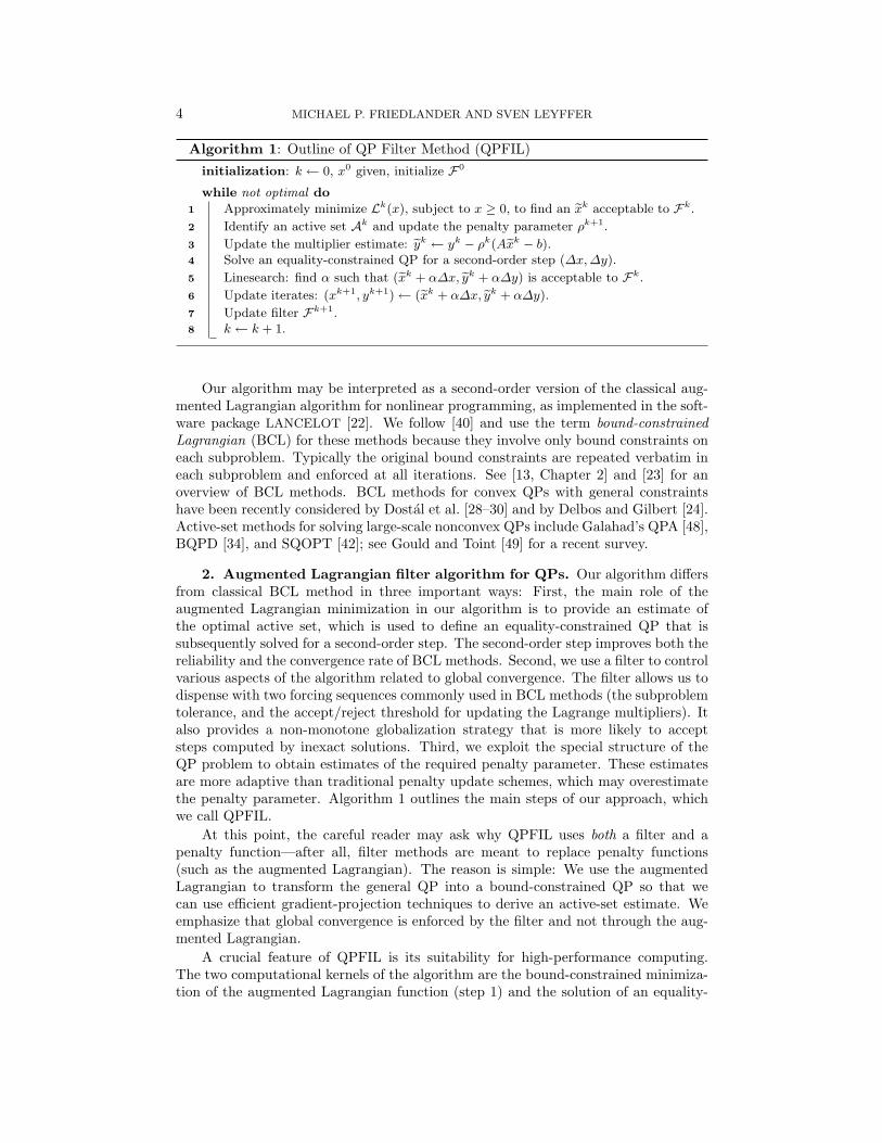
Algorithm 1: Outline of QP Filter Method (QPFIL)initialization: k ← 0, x0 given, initialize F0

while not optimal do

Approximately minimize Lk(x), subject to x ≥ 0, to find an exk acceptable to Fk.1

Identify an active set Ak and update the penalty parameter ρk+1.2

Update the multiplier estimate: eyk ← yk − ρk(Aexk − b).3

Solve an equality-constrained QP for a second-order step (∆x,∆y).4

Linesearch: find α such that (exk + α∆x, eyk + α∆y) is acceptable to Fk.5

Update iterates: (xk+1, yk+1)← (exk + α∆x, eyk + α∆y).6

Update filter Fk+1.7

k ← k + 1.8

Our algorithm may be interpreted as a second-order version of the classical aug-mented Lagrangian algorithm for nonlinear programming, as implemented in the soft-ware package LANCELOT [22]. We follow [40] and use the term bound-constrainedLagrangian (BCL) for these methods because they involve only bound constraints oneach subproblem. Typically the original bound constraints are repeated verbatim ineach subproblem and enforced at all iterations. See [13, Chapter 2] and [23] for anoverview of BCL methods. BCL methods for convex QPs with general constraintshave been recently considered by Dostal et al. [28–30] and by Delbos and Gilbert [24].Active-set methods for solving large-scale nonconvex QPs include Galahad’s QPA [48],BQPD [34], and SQOPT [42]; see Gould and Toint [49] for a recent survey.

2. Augmented Lagrangian filter algorithm for QPs. Our algorithm differsfrom classical BCL method in three important ways: First, the main role of theaugmented Lagrangian minimization in our algorithm is to provide an estimate ofthe optimal active set, which is used to define an equality-constrained QP that issubsequently solved for a second-order step. The second-order step improves both thereliability and the convergence rate of BCL methods. Second, we use a filter to controlvarious aspects of the algorithm related to global convergence. The filter allows us todispense with two forcing sequences commonly used in BCL methods (the subproblemtolerance, and the accept/reject threshold for updating the Lagrange multipliers). Italso provides a non-monotone globalization strategy that is more likely to acceptsteps computed by inexact solutions. Third, we exploit the special structure of theQP problem to obtain estimates of the required penalty parameter. These estimatesare more adaptive than traditional penalty update schemes, which may overestimatethe penalty parameter. Algorithm 1 outlines the main steps of our approach, whichwe call QPFIL.

At this point, the careful reader may ask why QPFIL uses both a filter and apenalty function—after all, filter methods are meant to replace penalty functions(such as the augmented Lagrangian). The reason is simple: We use the augmentedLagrangian to transform the general QP into a bound-constrained QP so that wecan use efficient gradient-projection techniques to derive an active-set estimate. Weemphasize that global convergence is enforced by the filter and not through the aug-mented Lagrangian.

A crucial feature of QPFIL is its suitability for high-performance computing.The two computational kernels of the algorithm are the bound-constrained minimiza-tion of the augmented Lagrangian function (step 1) and the solution of an equality-


constrained QP (step 4). Scalable tools that perform well on high-performance ar-chitectures exist for both steps. For example, TAO [9] and PETSc [3,4] are suitable,respectively, for the bound-constrained subproblem and the equality-constrained QP.In the remainder of this section we give details of each step of the QPFIL algorithm.

2.1. An augmented Lagrangian filter. The iterations of a BCL method fornonconvex optimization typically are controlled by two fundamental forcing sequencesthat ensure convergence to a solution. A decreasing sequence, ωk → 0, determinesthe required optimality of each subproblem solution and controls the convergence ofthe dual infeasibility (see (1.3a)). The second decreasing sequence, ηk → 0, tracksthe primal infeasibility (see (1.3b)) and determines whether the penalty parameter ρk

should be increased or left unchanged.In the definition of our filter we use quantities that are analogous to ωk and ηk:

ω(x, y) := ‖min{x,∇xL0(x, y)}‖,η(x) := ‖Ax− b‖,

which are based on the optimality and feasibility of a current pair (x, y). As we provein section 3, such a choice allows us to dispense with the sequences normally foundin BCL methods and instead defines these sequences implicitly. We observe that thefilter will generally be less conservative than BCL methods in the acceptance of acurrent subproblem solution or multiplier update.

Note that w(x, y) is based on the gradient of the Lagrangian function, not on theaugmented Lagrangian. Thus, our decision on when to exit the minimization of thecurrent subproblem is based on the optimality of the current subproblem iterate for theoriginal problem, rather than being based on the optimality of the current subproblem,as is usually the case in BCL methods. This approach ensures that the subproblemiterations (defined below) always generate solutions that are acceptable to the filter.Another advantage of this definition is that the filter is, in effect, independent of thepenalty parameter ρk and hence does not need to be updated if ρk is increased.

In the remainder of the paper we use the abbreviations

ωk := ω(xk, yk) and ηk := η(xk).

Definition 2.1 (augmented Lagrangian filter). The following rules define anaugmented Lagrangian filter:

1. A pair (ω′, η′) dominates another pair (ω, η) if ω′ ≤ ω and η′ ≤ η, and atleast one inequality holds strictly.

2. A filter F is a list of pairs (ω, η) such that no pair dominates another.3. A filter F contains an entry (called the upper bound)

(ω, η) = (U, 0), (2.1)

where U is a positive constant.4. A pair (x′, y′) is acceptable to the filter F if and only if

ω′ ≤ βω` or η′ ≤ βη` − γω′, (2.2)

for each (ω`, η`) ∈ F , where β, γ ∈ (0, 1) are constants.We use the shorthand notation ` ∈ F to imply that (ω`, η`) ∈ F .

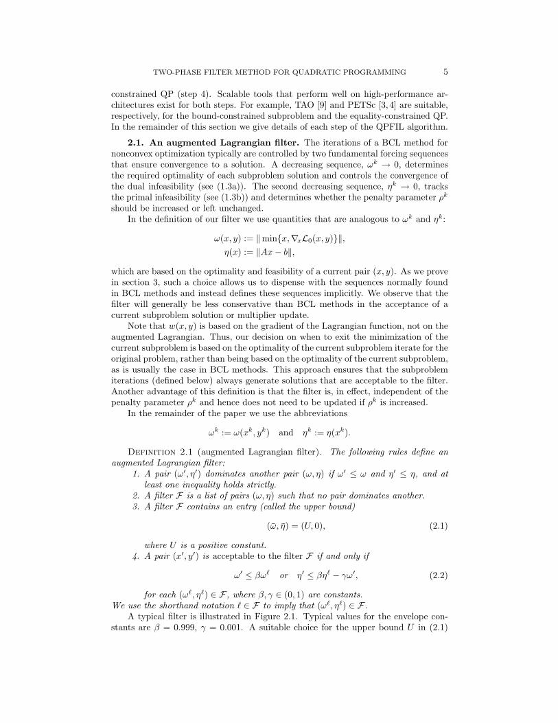
A typical filter is illustrated in Figure 2.1. Typical values for the envelope con-stants are β = 0.999, γ = 0.001. A suitable choice for the upper bound U in (2.1)


U ω(x, y)

upper bound

η(x)

Fig. 2.1. A typical filter. All pairs (ω, η) that are below and to the left of the envelope (dashedline) are acceptable to the filter (cf. (2.2)).

is U = δmax{1, ω0}, with δ = 1.25. Filter methods are typically insensitive to thechoice of these parameters, and most importantly, these parameters are not problem-dependent, unlike penalty parameters which must be chosen with more care. We notethat (2.2) creates a sloping envelope around the filter. Together with (2.1), this impliesthat a sequence {(ωk, ηk)} of pairs each acceptable to Fk must satisfy ωk → ω∗ = 0.If the second condition in (2.2) were weakened to ηk+1 ≤ βη`, then the sequence ofpairs acceptable to Fk could accumulate to points where ηk → η∗ = 0, but which arenonstationary because ωk → ω∗ > 0.

A consequence of η(x) ≥ 0 and the sloping envelope is that the upper bound(U, 0) is theoretically unnecessary—the sloping envelope implies an upper bound U =ηmin/γ, where ηmin is the least η` for all ` ∈ F . In practice, however, we impose theupper bound U in order to avoid generating entries with excessively large values ωk.

We remark that the axes in the augmented Lagrangian filter appear to be thereverse of the usual definition: feasibility is on the vertical axis instead of the hori-zontal axis, as it typically appears in the literature. This reflects the dual view of theaugmented Lagrangian: it can be shown that Ax − b is a steepest descent directionat x for the augmented Lagrangian [14, §2.2], and that ω(x, y) is the dual feasibilityerror. This definition of the filter is similar to the one used in [45]. The gradient ofthe Lagrangian has also been used in the filter by Ulbrich et al. [59], together with acentrality measure, in the context of interior-point methods.

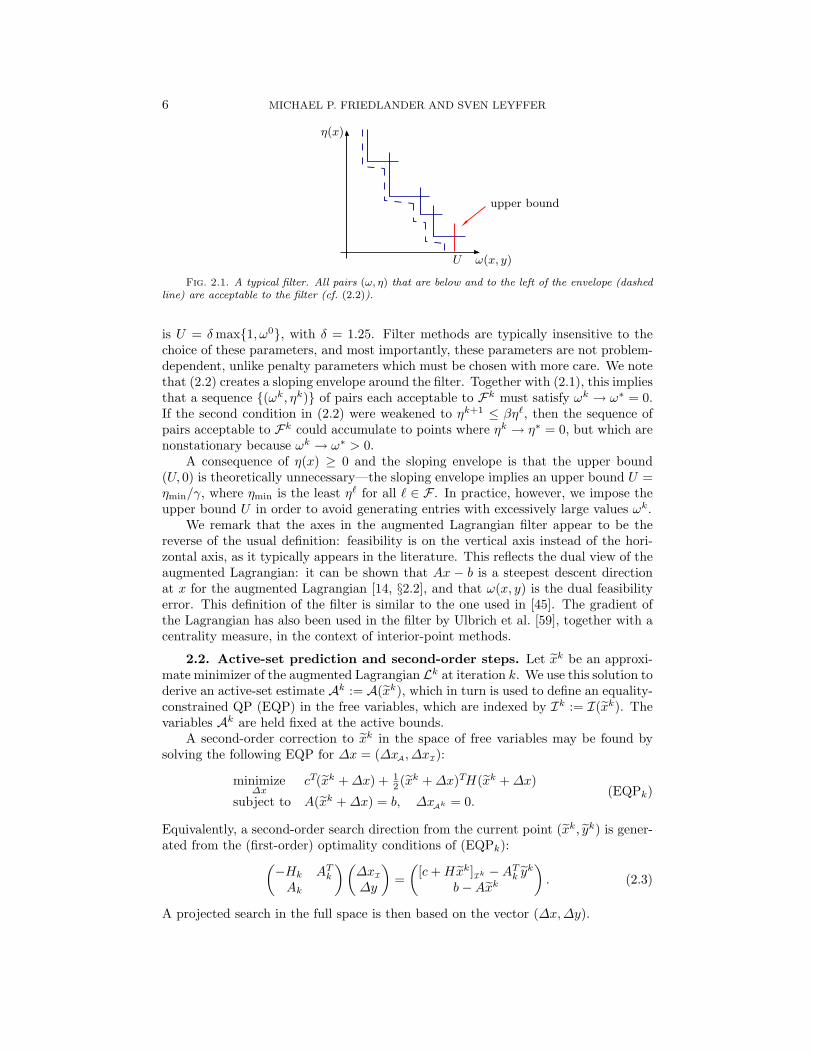
2.2. Active-set prediction and second-order steps. Let xk be an approxi-mate minimizer of the augmented Lagrangian Lk at iteration k. We use this solution toderive an active-set estimate Ak := A(xk), which in turn is used to define an equality-constrained QP (EQP) in the free variables, which are indexed by Ik := I(xk). Thevariables Ak are held fixed at the active bounds.

A second-order correction to xk in the space of free variables may be found bysolving the following EQP for ∆x = (∆xA, ∆xI):

minimize∆x

cT(xk +∆x) + 12 (xk +∆x)TH(xk +∆x)

subject to A(xk +∆x) = b, ∆xAk = 0.(EQPk)

Equivalently, a second-order search direction from the current point (xk, yk) is gener-ated from the (first-order) optimality conditions of (EQPk):(

−Hk ATkAk

)(∆xI∆y

)=(

[c+Hxk]Ik −ATk ykb−Axk

). (2.3)

A projected search in the full space is then based on the vector (∆x,∆y).


ρρmin

y∗

y

D

(a) Nonlinear constraints

ρρmin

y

D

(b) Linear constraints

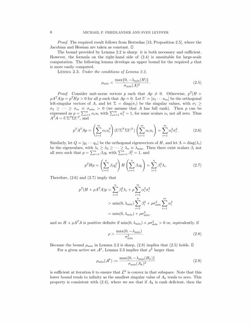
Fig. 2.2. The sets D illustrate the required penalty parameter for the BCL method when theconstraints are either nonlinear or linear.

Note that step 1 of Algorithm 1 requires that the approximate augmented La-grangian minimizer xk be acceptable to the filter. Moreover, as we demonstrate insection 3.2, the first-order multiplier estimate yk must also be acceptable to the filter.These two properties ensure that even if a linesearch along (∆x,∆y) fails to obtain apositive steplength α such that (xk + α∆x, yk + α∆y) is acceptable to the filter, thealgorithm can still make progress with the first-order step alone. In this case, α = 0,and the algorithm relies on the progress of the standard BCL iterations.

2.3. Estimating the penalty parameter. It is well known that BCL meth-ods, under standard assumptions, converge for all large-enough values of the penaltyparameter ρk. The threshold value ρmin is never computed explicitly; instead, BCLmethods attempt to discover the threshold value by increasing ρk in stages. Typicallythe norm of the constraint violation is used to guide the decisions regarding when toincrease the penalty parameter: a linear decrease (as anticipated by the BCL localconvergence theory) signals that the penalty parameter may be held constant; lessthan linear convergence—or a large increase in constraint violations—indicates thata larger ρk is needed.

When the constraints are nonlinear, the penalty-parameter threshold and theinitial Lagrange multiplier estimates are closely coupled. Poor estimates yk of y∗

imply that a larger ρk is needed to induce convergence. This coupling is fully de-scribed by Bertsekas [13, Proposition 2.4]. When the constraints are linear, however,the Lagrange multipliers do not appear in (1.2b), and we see that yk and ρk areessentially decoupled—the curvature of Lk can be influenced by changing ρk alone.This observation is illustrated in Figure 2.2, in which the left figure corresponds tononlinear constraints and the right figure to linear constraints. The regions in thepenalty/multiplier plane for which BCL methods converge are indicated by the shadedregions D. The result below provides an explicit threshold value ρmin needed to ensurethat the Hessian of the augmented Lagrangian is positive definite (a positive multipleof ρmin is enough to induce convergence). Let λmin(·) and σmin(·), respectively, denotethe leftmost eigenvalue, and the smallest singular value, of a matrix.

Lemma 2.2. Suppose that pTHp > 0 for all nonzero p such that Ap = 0 and Ahas full row rank. Then H + ρATA is positive definite if and only if

ρ > ρmin := λmin

(A(H + γATA)−1AT

)−1 − γI, (2.4)

for any γ ≥ 0 such that H + γATA is nonsingular.


Proof. The required result follows from Bertsekas [13, Proposition 2.5], where theJacobian and Hessian are taken as constant.

The bound provided by Lemma 2.2 is sharp: it is both necessary and sufficient.However, the formula on the right-hand side of (2.4) is unsuitable for large-scalecomputation. The following lemma develops an upper bound for the required ρ thatis more easily computed.

Lemma 2.3. Under the conditions of Lemma 2.2,

ρmin <max{0,−λmin(H)}

σmin(A)2. (2.5)

Proof. Consider unit-norm vectors p such that Ap 6= 0. Otherwise, pT(H +ρATA)p = pTHp > 0 for all p such that Ap = 0. Let U = [u1 · · ·um] be the orthogonalleft-singular vectors of A, and let Σ = diag(σi) be the singular values, with σ1 ≥σ2 ≥ · · · ≥ σm ≡ σmin > 0 (we assume that A has full rank). Then p can beexpressed as p =

∑mi=1 αiui with

∑mi=1 α

2i = 1, for some scalars αi not all zero. Thus

ATA = UΣTΣUT, and

pTATAp =

(m∑i=1

αiuTi

)(UΣTΣUT )

(m∑i=1

αiui

)=

m∑i=1

α2iσ

2i . (2.6)

Similarly, let Q = [q1 · · · qn] be the orthogonal eigenvectors of H, and let Λ = diag(λi)be the eigenvalues, with λ1 ≥ λ2 ≥ · · · ≥ λn ≡ λmin. Then there exist scalars βi notall zero such that p =

∑ni=1 βiqi with

∑ni=1 β

2i = 1, and

pTHp =

(n∑i=1

βiqTi

)H

(n∑i=1

βiqi

)=

n∑i=1

β2i λi. (2.7)

Therefore, (2.6) and (2.7) imply that

pT(H + ρATA)p =n∑i=1

β2i λi + ρ

m∑i=1

α2iσ

2i

> min(0, λmin)n∑i=1

β2i + ρσ2

min

m∑i=1

α2i

= min(0, λmin) + ρσ2min,

and so H + ρATA is positive definite if min(0, λmin) + ρσ2min > 0 or, equivalently, if

ρ >max(0,−λmin)

σ2min

. (2.8)

Because the bound ρmin in Lemma 2.2 is sharp, (2.8) implies that (2.5) holds.For a given active set Ak, Lemma 2.3 implies that ρk larger than

ρmin(Ak) :=max{0,−λmin(Hk)}

σmin(Ak)2(2.9)

is sufficient at iteration k to ensure that Lk is convex in that subspace. Note that thislower bound tends to infinity as the smallest singular value of Ak tends to zero. Thisproperty is consistent with (2.4), where we see that if Ak is rank deficient, then the


required bound in Lemma 2.2 does not exist. In section 3 we show that for a givenoptimal active set, a multiple of this bound is required to induce convergence to anoptimal solution in our method.

We are not entirely satisfied with (2.9) because it requires an estimate (or at leasta lower bound) of the smallest singular value of the current Ak which can be relativelyexpensive to compute. One possibility for estimating this value is to use a Lanczosbidiagonalization procedure, as implemented in PROPACK [51].

Ideally, we would compute the penalty value according to (2.4) or (2.5). However,for the size of problems of interest, this approach would be prohibitive in terms ofcomputational effort. In our numerical experiments we have instead used the quantity

ρmin(Ak) = max

1,‖Hk‖1

max{

1√|Ik|‖Ak‖∞ , 1√

m‖Ak‖1

} ,

where |Ik| is the number of free variables and m is the number of general equalityconstraints, as a simple approximation to (2.9). We note that the penalty parameteronly appears within the subproblem minimization (step 1 of Algorithm 1), and not inthe definition of the filter. If only a rough approximation to (2.9) is available, thena multiple of the approximation might be used so as to increase the likelihood thata large-enough quantity is obtained. In the remainder of the paper, we assume thatρmin(Ak) is given by (2.9).

2.4. Minimizing the augmented Lagrangian subproblem. Like classicalBCL methods, our method generates a sequence of approximate minimizers of thebound-constrained subproblem

minimizex

Lk(x) subject to x ≥ 0. (2.10)

Instead of optimizing the subproblem to a prescribed tolerance, however, each itera-tion of the inner algorithm approximately optimizes it in stages (i.e., a few iterationsof some minimization procedure are applied), so that at each iteration j of the inneralgorithm, the current iterate xj satisfies the approximate optimality conditions

‖min{x,∇xLρj (x, y)}‖∞ ≤ εj , (2.11)

where y is the latest multiplier estimate yk. The only requirement for the sequence ofapproximate minimizations is that they eventually solve the subproblem in the limit,and thus that εj → 0. The iterate xj and the implied first-order multiplier (1.1) aretested for acceptability against the current filter. The inner-minimization algorithmis described in Algorithm 2.

The penalty parameter ρj is checked at each inner iteration to ensure that itsatisfies the bound implied by Lemma 2.2 (see steps 5 and 7). If the current submatrixAj is rank deficient (i.e., σmin(Aj) = 0), then there does not exist a finite ρ that makesthe reduced Hessian positive definite. In that case, we are not assured that reducingthe augmented Lagrangian brings the next iterate any closer to optimality of theoriginal subproblem. Instead, we make progress towards feasibility of the iterates byapproximately solving the minimum infeasibility problem

minimizex

12‖Ax− b‖

2 subject to x ≥ 0, (2.12)


Algorithm 2: Bound-Constrained Lagrangian Filter (BCLFIL)Inputs: x0, y, ρ1, F Outputs: ex, ey, eρSet α ∈ [0, 1), j ← 0repeat

j ← j + 11

Choose εj > 0 such that limj→∞ εj = 02

Find a point xj that satisfies (2.11) [approximately solve (2.10)]3

Aj ← A(xj) [update active set]4

if σmin(Aj) = 0 then5

Find a point xj that satisfies (2.13) [feasibility restoration]6

else if ρj < 2ρmin(Aj) then7

ρj+1 ← 2ρmin(Aj) [increase penalty parameter]8

else9

yj ← y − ρj(Axj − b) [provisional multiplier update]10

(ωj , ηj)←`ω(xj , yj), η(xj)

´[update primal-dual infeasibility]11

if (ωj , ηj) is acceptable to F then12

return ex← xj , ey ← yj , eρ← ρj

ρj+1 ← ρj [keep penalty parameter]13

until converged

and we thus require that xj satisfy the approximate necessary and sufficient condition

‖min{x,AT(Ax− b)}‖∞ ≤ εj . (2.13)

The point xj ≥ 0 solves the minimum infeasibility problem if ATj (AjxjIj − b) = 0,

which can be satisfied at infeasible points if Aj is rank deficient.An alternative to step 6 of Algorithm 2 is to increase ρj by a fixed multiple. A

similar strategy is used in the method suggested in [30], where ρj is increased if thecurrent iterate is not “extended regular.” With this update, it can be shown that ifρj →∞, then every limit point x∗ of xj is either a KKT point of (GQP) or a solutionof (2.12) (see Theorem 7.1). The analysis given in [30] shows that x∗ continues tobe a solution of the original QP, but this conclusion depends crucially on the strictconvexity of (GQP)—an assumption that we do not make here.

In classical BCL methods, the gradient of the augmented Lagrangian at the latestiterate xj and the latest multiplier estimate y is used to test termination of the inneriterations. The test in step 12 of Algorithm 2 is based on the norm of the (usual)Lagrangian function at xj , but it differs from BCL in using the first-order multiplierestimate yj = y−ρj(Axj− b). We note that the identity ∇xLρj (xj , y) = ∇xL0(xj , yj)implies that the quantities used to test termination in Algorithm 2 and in classicalBCL methods are in fact identical. Algorithm 2 additionally uses the current primalinfeasibility ηj as a criterion. The inner minimization terminates when the currentiterates are acceptable to the filter and the penalty parameter is large enough for thecurrent active set.

To establish that our algorithm finitely identifies the optimal active set (see sec-tion 4), we assume that each approximate minimization reduces the objective by atleast as much as does a Cauchy point of a projected-gradient method (see, e.g., [57,§16.6]). This is a mild assumption that is satisfied by most globally convergent bound-constrained solvers. In practice, we perform one or two steps of a bound-constrainedoptimization algorithm and then test the acceptability of (ωj , ηj) to the filter. This


Algorithm 3: QP Filter Method (QPFIL)Inputs: x0, y0 Outputs: x∗, y∗

Set penalty parameter ρ0 > 0 and positive filter envelope parameters β, γ < 1.Set filter upper bound U ← γmax

˘1, ‖Ax0 − b‖

¯, and add (U, 0) to filter F0.

Set minimum steplength αmin > 0.Compute infeasibilities ω0 ← ω(x0, y0) and η0 ← η(x0).k ← 0if ω0 > 0 and η0 > 0 then add (ω0, η0) to F0.1

while not optimal dok ← k + 12

(exk, eyk, ρk)← BCLFIL(xk−1, yk−1, ρk−1,Fk−1)3

Ak ← A(exk)4

Find (∆xk,∆yk) that solves (2.3)5

Find αk ∈ [αmin, 1] such that (exk + α∆xk, eyk + α∆yk) is acceptable to Fk6

if linesearch failed then7

(xk, yk)← (exk, eyk) [keep first-order iterates]8

else

(xk, yk)← (exk + αk∆xk, eyk + α∆yk) [second-order update]9

(ωk, ηk)←`ω(xk, yk), η(xk)

´[compute infeasibilities]10

if ωk > 0 then11

Fk ← Fk−1 ∪ {(ωk, ηk)}12

Remove redundant entries from Fk13

if ηk = 0 then update upper bound U14

return x∗ ← xk, y∗ ← yk

requirement is often weaker than traditional augmented Lagrangian methods, whichat each outer iteration must reduce the projected gradient beyond a specified toler-ance that goes to zero; in contrast, here the inner-iteration tolerances are independentacross outer iterations.

2.5. Detailed algorithm statement. The proposed algorithm is structuredaround outer and inner iterations. The outer iterations handle management of thefilter, the solution of (EQPk), and the subsequent linesearch. The inner iterationsminimize the augmented Lagrangian function, update the multipliers and the penaltyparameter, and identify a candidate set of active constraints used to define (EQPk)for the outer iteration. Thus, each inner iteration performs steps 1–3 of Algorithm 1.

In step 6 of Algorithm 3 we perform a filter linesearch by trying a sequence ofsteps α = γi, i = 0, 1, 2, . . ., for some constant γ ∈ (0, 1) until an acceptable point isfound, or until α < αmin, where αmin > 0 is a constant parameter. The parameterαmin is needed because the first-order point (xk, yk) could lie in a corner of the filterwith the second-order step implying a step into the filter. In that case there existsno α > 0 that yields an acceptable step. Other ways of deciding when to terminatethe linesearch are possible, based, for example, on requiring that the new filter areainduced by the linesearch step be larger than the new filter area induced by thefirst-order step.

The filter update in step 12 of Algorithm 3 removes redundant entries that aredominated by a new entry. The upper bound (U, 0) also allows us to manage thenumber of filter entries that we wish to store. If this number is exceeded, then we


can reset the upper bound as U = max`{ω` | ω` ∈ Fk} and subsequently deletedominated entries from Fk, thus reducing the number of filter entries.

3. Global convergence. Global convergence of Algorithm 3 (QPFIL) is basedon progress made by the inner iterations of step 3. The second-order updates insteps 5–9 serve only to accelerate convergence. Therefore, we can establish globalconvergence of QPFIL by analyzing a first-order version of the algorithm that does notuse the second-order updates. The following assumption holds implicitly throughout.

Assumption 3.1. The sequences {xj} and {xk} generated by Algorithms 2 and 3lie in a compact set. Hence, each sequence has at least one limit point.

3.1. Preliminaries. When A∗ has full rank, define the least-squares multiplierestimate y(x) as the unique solution of the least-squares problem

y(x) := arg miny

‖[c+Hx]I∗ −AT∗y‖. (3.1)

Because the least-squares multiplier estimate is unique, there exists a positive constantα1 such that

‖y(x)− y(x∗)‖ ≤ α1‖x− x∗‖. (3.2)

Note that the definition of y requires a priori knowledge of the bounds that are activeat the solution; however, y is used only for analysis and is never computed.

Lemma 3.2. Suppose that A∗ has full rank and y is an approximate least-squaressolution of (3.1) for some x. Then there exists a positive constant α2 such that

‖y(x)− y‖ ≤ α2‖[c+Hx]I∗ −AT∗y‖. (3.3)

Proof. Let r(x) and r be the least-squares residuals associated with y(x) and y,respectively, so that AT∗y(x) + r(x) = [c+Hx]I∗ and AT∗y + r = [c+Hx]I∗ . Then

AT∗(y(x)− y) + r(x)− r = 0,

and because A∗r(x) = 0, it follows that A∗AT∗(y(x) − y) + A∗r = 0. Because A∗

has full rank, it is straightforward to show that there exists a positive constant α2

such that ‖y(x) − y‖ ≤ α2‖r‖, and the required result follows immediately from thedefinition of r.

The next result shows how a sequence of multiplier estimates is related to theleast-squares multiplier estimates.

Lemma 3.3. Let {ωk} and {ρk} be sequences of positive scalars where ωk → 0.Let {xk} and {yk} be any sequences of n-vectors and m-vectors, respectively, thattogether satisfy

‖min{xk,∇xL0(xk, yk)}‖∞ ≤ ωk. (3.4)

Let x∗ be any limit point of {xk} with an associated sequence of indices K. Supposethat A∗ has full rank and let y∗ := y(x∗). Then there are positive constants α1 andα2 such that

‖yk − y∗‖ ≤ βk := α1‖xk − x∗‖+ α2ωk, (3.5)

for all k ∈ K large enough.


Proof. Set zk := ∇xL0(xk, yk). For k ∈ K large enough, xk is sufficiently close tox∗ that xki > 0 if x∗i > 0. Then for such k, (3.4) and ωk → 0 imply that min{xki , zki } =z∗i , so that

‖zkI∗‖ ≤ ‖min{xk, zk}‖ ≤√n ωk. (3.6)

We now derive (3.5). From the triangle inequality,

‖yk − y∗‖ ≤ ‖y(xk)− yk‖+ ‖y(xk)− y∗‖. (3.7)

Also, (3.3) (with x = xk and y = yk) and (3.6) together imply that

‖y(xk)− yk‖ ≤ α2ωk.

Substituting this and (3.2) (with x = xk) into (3.7), we obtain (3.5).

3.2. Convergence of inner iterations. We expect that the usual behavior ofAlgorithm 2 will be to terminate finitely. However, as the next theorem proves, if thealgorithm does not terminate, then the inner iterations converge to a KKT point of(GQP), or they converge to a solution of the minimum infeasibility problem (2.12).For this section only, let

yj := y − ρj(Axj − b) and zj := ∇xL0(xj , yj).

Theorem 3.4 (convergence of inner iterations). Let {xj} and ρk be sequencesgenerated by Algorithm 2. Then the algorithm terminates finitely, or every limit pointx∗ of {xj} is a KKT point of (GQP), or solves (2.12).

Proof. We first consider the case where step 5 tests true finitely many times andthen treat separately the two other cases where step 5 tests true infinitely many times(and hence ρj →∞) and A∗ is either full rank or not.

Case 1. (Step 5 test true finitely many times.) In this case, the alternativesteps 7 or 9 must evaluate true for all j large enough. But there are only finitelymany different active sets, and so step 5 can evaluate true only finitely many times.Hence, {ρj} remains bounded and step 12 is tested for all j large enough. Consideronly such j. Because each xj satisfies (2.11), steps 10 and 11 ensure that ωj → 0.Moreover, for every ` ∈ F , ω` > 0 (see steps 1 and 11 of Algorithm 3), and soωj must be acceptable to the filter (see (2.2)) after finitely many iterations. Hence,Algorithm 2 exits finitely.

Case 2. (Step 5 test true infinitely many times.) In this case, each xj in somesub-sequence J satisfies (2.13). Because εj → 0, the limit point x∗ associated withthe sequence J satisfies (2.13), and it must therefore be a solution of (2.12).

In Theorem 7.1 (see section 7) we give an analogous convergence proof for aslightly modified version of Algorithm 2 that offers alternative to steps 5–6. See [1]for a related convergence analysis that relies on a set of different assumptions.

The hypotheses of Theorem 3.4 can fail to hold if there are no convergent sub-sequences (i.e., Assumption 3.1 fails to hold) or if Algorithm 2 breaks down becauseno iterate xj can be found to satisfy the stopping condition (2.11). For example,the subproblem is unbounded below, which can happen if there exists a nonzero andnonnegative vector d such that dTHd < 0 and Ad = 0.


3.3. Convergence of first-order algorithm. For this section only, we con-sider a simplified algorithm that skips the second-order update (steps 5–10 of Algo-rithm 3). In this case, (xk, yk) ≡ (xk, yk), and we refer to the sequence {(xk, yk)}of augmented Lagrangian minimizers and multiplier estimates as Cauchy points; ourintent is to emphasize that these solutions can be interpreted as steepest-ascent stepsof the augmented Lagrangian function and thus can yield only linear convergence.

We prove that the first-order sequence {(xk, yk)} generated in step 3 converges toa stationary point of (GQP). This result is of interest also within the context of moreestablished BCL methods because it illustrates how a filter can be used in place ofthe two arbitrary forcing sequences (ωk and ηk) commonly associated with augmentedLagrangian methods.

We show the sequence of penalty parameters ρk is bounded, and that every limitpoint of the primal-dual pair (xk, yk) satisfies (1.3a) and is thus dual feasible.

Lemma 3.5. The penalty parameter is updated finitely often.Proof. This follows from the fact that there exist only a finite number of different

active sets that could result in a penalty-parameter update.Lemma 3.6. Any limit point (x∗, y∗) of {(xk, yk)} satisfies ωk ≡ ω(xk, yk)→ 0.Proof. We consider two mutually exclusive cases, depending on whether a finite

or an infinite number of entries are added to the filter. If a finite number of entriesare added to the filter (i.e., if step 11 of Algorithm 3 tests true only finitely manytimes), then it follows that ωk = 0 for all k sufficiently large. The required result thenfollows immediately. If, on the other hand, an infinite number of entries (ωk, ηk) areadded to the filter, then the required result follows from [19, Lemma 1]—where wetake f(x) = η(x) and h(x) = ω(x, y)—because η(x) is trivially bounded below.

The following theorem is our main convergence result on the sequence of Cauchypoints.

Theorem 3.7 (global convergence with single limit point). Consider a version ofAlgorithm 3 that skips steps 5–10. Assume that the algorithm generates a sequence ofCauchy points {(xk, yk)}, and that x∗ is the single limit point of {xk}. Then yk → y∗,where y∗ := y(x∗), and (x∗, y∗) is a KKT point of (GQP).

Proof. Step 3 of Algorithm 3, together with Lemma 3.6, ensure that each xk, yk,ρk, and ωk, for k ∈ K, satisfy the conditions of Lemma 3.3. Then (3.4)–(3.5) hold,and yk → y∗, as required. Because ωk → 0, (3.4) implies that

0 ≤ limk→∞

‖min{xk,∇xL0(xk, yk)}‖∞ ≤ limk→∞

ωk = 0,

and so min{x∗,∇xL0(x∗, y∗)} = 0. Therefore, (x∗, y∗) satisfies (1.3a).The “single limit point” assumption on xk and the definition of yk = yk−1 −

ρk(Axk− b) (see step 10 of Algorithm 2) imply that ‖yk−yk−1‖ → 0. By Lemma 3.5,ρk is bounded for all k, so

‖yk − yk−1‖ = ρk‖Axk − b‖ → 0, (3.8)

and x∗ satisfies (1.3b). Hence, (x∗, y∗) is a KKT pair of (GQP).Recall that (GQP) is nonconvex, and hence the subproblem may have many

stationary points. The single-limit-point assumption of Theorem 3.7 excludes thesituation in which consecutive minimizations of the augmented Lagrangian subprob-lem converge to different stationary points. Otherwise, the corresponding Lagrangemultiplier updates would not have a limit point and (3.8) would not hold. We couldrelax the single-limit-point assumption if we instead assume that the subproblem


solver finds a stationary point closest in norm to xk. Such a requirement cannot beverified in practice, but depending on the subproblem solver, it is, arguably, often sat-isfied. A similar assumption is made implicitly in a classical proof of convergence ofthe augmented Lagrangian method: Bertsekas [13, Proposition 2.4] assumes that allminimizers of the augmented Lagrangian fall within a small neighborhood. The single-limit-point assumption made in Theorem 3.7 considerably simplifies the analysis andleads to similar conclusions. In the case where (GQP) is convex, every subproblemhas a unique minimizer and neither assumption is required.

If we instead assume that a second-order sufficiency condition exists at a limitpoint x∗, we can drop the single-limit-point assumption. In effect, the followingtheorem shows that second-order points are attractors, and the algorithm generatesincreasingly better Lagrange-multiplier estimates.

Theorem 3.8 (global convergence with second-order sufficiency). Consider aversion of Algorithm 3 that skips steps 5–10. Assume that the algorithm generates asequence of Cauchy points {(xk, yk)}, and that a limit point x∗ satisfies the second-order sufficiency condition

pTHp > 0 for all p 6= 0 satisfying Ap = 0 with pj = 0 for all j ∈ A∗. (3.9)

Then there exist positive constants δ1, δ2, δ3, and a positive constant γ < 1 such that

‖yk − y∗‖ ≤ δ1ωk + γ‖yk−1 − y∗‖, (3.10a)

‖xk − x∗‖ ≤ δ2ωk + δ3‖yk−1 − y∗‖, (3.10b)

ρk‖Axk − b‖ ≤ δ1ωk + (γ + 1)‖yk−1 − y∗‖, (3.10c)

where (x∗, y∗) is a KKT point of (GQP).Proof. Step 3 of Algorithm 3 together with Lemma 3.6 ensure that each xk, yk,

ρk, and ωk, for k ∈ K, satisfy the conditions of Lemma 3.3. Therefore, (3.6) holds,and by a symmetric argument, xkA∗ satisfies a similar inequality, and so

‖zkI∗‖ ≤√n ωk and ‖xkA∗‖ ≤

√n ωk. (3.11)

Note that each xk, yk, and zk satisfies

c+Hxk −ATyk = zk and yk = yk−1 − ρk(Axk − b).

Rearranging terms, we have(−Hk ATkAk

1ρk I

)(xkI∗yk

)=(

[c− zk]I∗1ρk y

k−1 + b

). (3.12)

Now consider the equality QP (cf. (EQPk))

minimizex

cTI∗x+ 12x

THkx subject to Akx = b,

which has optimality conditions(−Hk ATkAk

)(x∗I∗y∗

)=(cI∗

b

). (3.13)

Subtracting (3.12) from (3.13), we get(−Hk ATkAk

1ρk I

)([xk − x∗]I∗yk − y∗

)=(

−zkI∗1ρk (yk−1 − y∗)

). (3.14)


Note that this matrix is nonsingular if and only if Hk := H + ρkATkAk is nonsingular[37, Proposition 2]. But Algorithm 2 exits only if ρk > 2ρmin(Ak), and by Lemma 2.3and (3.9), Hk is in fact positive definite. Therefore, the solutions to (3.13) and (3.14)are unique. Moreover, inverting (3.14), we arrive at(

[xk − x∗]I∗yk − y∗

)=

(−H−1

k ρkH−1k ATk

ρkAkH−1k ρkI − (ρk)2AkH

−1k ATk

)(−zkI∗

1ρk (yk−1 − y∗)

). (3.15)

Apply the triangle inequality to the second equation to arrive at

‖yk − y∗‖ ≤ ρk‖AkH−1k ‖︸︷︷︸

(a)

‖zkI∗‖+ ‖I − ρkAkH−1k ATk ‖︸︷︷︸

(b)

‖yk−1 − y∗‖. (3.16)

Because ρk is bounded and Hk is positive definite, there exists a positive constant δ1that bounds (a). Next, note that AkH

−1k ATk = (A+T

k HkA+k + ρkI)−1. If λi are the

eigenvalues of A+Tk HkA

+k , then

ρk > 2max{0,−λmin(Hk)}

σmin(Ak)> 2 min

iλi.

Therefore,

‖I − ρkAkH−1k ATk ‖ = max

i

(1− ρk

λi + ρk

)= max

i

(λi

λi + ρk

)< 1,

and so we have a bound on (b). Together with (3.11) and (3.16), this implies that(3.10a) holds.

In order to derive (3.10b), we first observe that (3.11) implies that

‖xk − x∗‖ ≤√n ωk + ‖[xk − x∗]I∗‖. (3.17)

Also, from the first set of equations in (3.15),

‖[xk − x∗]I∗‖ ≤ ‖H−1k ‖ ‖z

kI∗‖+ ρk‖H−1

k ATk ‖ ‖yk−1 − y∗‖.

Substitute (3.10a) into the above, and subsequently substitute the result into (3.17)to obtain (3.10b).

To derive (3.10c), use the definition yk and the triangle inequality to derive thebound

ρk‖Axk − b‖ = ‖yk−1 − yk‖ ≤ ‖yk − y∗‖+ ‖yk−1 − y∗‖.

Substituting (3.10a) into the above and rearranging terms, we arrive at (3.10c).It is important to note that the conclusion of Theorem 3.8 does not imply linear

convergence of the Lagrange multiplier estimates. However, it still holds that yk → y∗:repeatedly apply (3.10a) to obtain

‖yk+` − y∗‖ ≤ δ1∑i=1

γ`−iωk+i−1 + γ`‖yk − y∗‖

for ` ≥ 1. Because ωk → 0 and γ < 1, it follows that yk+` → y∗ as ` → ∞. Thus,yk → y∗, and with (3.10b) and (3.10c), xk → x∗ and ‖Axk − b‖ → 0.


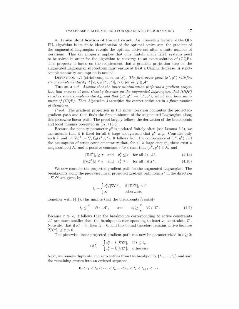
4. Finite identification of the active set. An interesting feature of the QP-FIL algorithm is its finite identification of the optimal active set: the gradient ofthe augmented Lagrangian reveals the optimal active set after a finite number ofiterations. This key property implies that only finitely many KKT systems needto be solved in order for the algorithm to converge to an exact solution of (GQP).This property is based on the requirement that a gradient projection step on theaugmented Lagrangian subproblem must ensure at least a Cauchy decrease. A strict-complementarity assumption is needed.

Definition 4.1 (strict complementarity). The first-order point (x∗, y∗) satisfiesstrict complementarity if [∇xL0(x∗, y∗)]i > 0 for all j ∈ A∗.

Theorem 4.2. Assume that the inner minimization performs a gradient projec-tion that ensures at least Cauchy decrease on the augmented Lagrangian, that (GQP)satisfies strict complementarity, and that (xk, yk) → (x∗, y∗), which is a local mini-mizer of (GQP). Then Algorithm 3 identifies the correct active set in a finite numberof iterations.

Proof. The gradient projection in the inner iteration computes the projected-gradient path and then finds the first minimum of the augmented Lagrangian alongthis piecewise linear path. The proof largely follows the derivation of the breakpointsand local minima presented in [57, §16.6].

Because the penalty parameter ρk is updated finitely often (see Lemma 3.5), wecan assume that it is fixed for all k large enough and that ρk ≡ ρ. Consider onlysuch k, and let ∇Lk := ∇xL0(xk, yk). It follows from the convergence of (xk, yk) andthe assumption of strict complementarity that, for all k large enough, there exist aneighborhood Nε and a positive constant τ � ε such that (xk, yk) ∈ Nε and

[∇Lk]i ≥ τ and xki ≤ ε for all i ∈ A∗, (4.1a)

|[∇Lk]i| ≤ ε and xki ≥ τ for all i ∈ I∗. (4.1b)

We now consider the projected gradient path for the augmented Lagrangian. Thebreakpoints along the piecewise linear projected gradient path from xk in the direction−∇Lk are given by

ti =

{xki /[∇Lk]i if [∇Lk]i > 0∞ otherwise.

Together with (4.1), this implies that the breakpoints ti satisfy

ti ≤ε

τ∀i ∈ A∗, and ti ≥

τ

ε∀i ∈ I∗. (4.2)

Because τ � ε, it follows that the breakpoints corresponding to active constraintsA∗ are much smaller than the breakpoints corresponding to inactive constraints I∗.Note also that if xki = 0, then ti = 0, and this bound therefore remains active because[∇Lk]i ≥ τ > 0.

The piecewise linear projected gradient path can now be parameterized in t ≥ 0:

xi(t) =

{xki − t [∇Lk]i if t ≤ ti,xki − ti[∇Lk]i otherwise.

Next, we remove duplicate and zero entries from the breakpoints {t1, . . . , tn} and sortthe remaining entries into an ordered sequence

0 < t1 < t2 < · · · < ta−1 < ta < ti < ti+1 < · · · .


Observe that (4.2) implies that this ordering separates the active indices 1, . . . , a fromthe inactive indices i, i+ 1, . . ., and that

ta ≤ε

τ� τ

ε≤ ti.

We now show that the first minimizer of the augmented Lagrangian occurs in theinterval [ta, ti] for ε sufficiently small, and therefore the correct active set is identified.We must first demonstrate that the augmented Lagrangian has no minimizer in anyof the intervals [tj−1, tj ] for j ≤ a. Let j ≤ a, and consider the piecewise searchdirection on [tj−1, tj ]:

pj−1i =

{−[∇Lk]i if tj−1 ≤ ti,0 otherwise.

(4.3)

Next, consider the path segment given by

x(t) = x(tj−1) +∆t pj−1 for ∆t ∈ [0, tj − tj−1],

and look for a minimizer of the augmented Lagrangian in this segment. We expandthe Lagrangian along this segment and compute the directional gradient on [tj−1, tj ]:

−f ′j−1 = −(∇Lk)Tpj−1 − x(tj−1)T(H + ρATA)pj−1.

From (4.1a) and (4.3), it follows that the first term on the right-hand side above isbounded below by τ2, whereas the second term is O(ετ). Therefore, the first termdominates, and −f ′j−1 ≥ τ2 for j ≤ a+ 1.

Next, observe that the directional Hessian on [tj−1, tj ],

f ′′j−1 = pj−1(H + ρATA)pj−1,

is bounded because H + ρATA and pj−1 are bounded. Using (4.1a) and (4.3), weconclude that there exist positive constants κ1 and κ2, independent of ε, such thatκ1τ

2 ≤ f ′′j−1 ≤ κ2. Because f ′′j−1 > 0, the minimizer of the augmented Lagrangian onthe segment [tj−1, tj ] is given by

t∗j = min{−f ′j−1

f ′′j−1

, tj − tj−1

}.

The first term in the minimum can be bounded below by τ2/κ2 � ε, and the secondterm is O(ε). Thus, for ε sufficiently small, the minimum of the quadratic on thesegment [tj−1, tj ] occurs at tj for all j ≤ a, and the projected gradient search proceedsto the next segment, [tj , tj+1]. Repeating this argument for all j ≤ a shows that thereis no minimum of the augmented Lagrangian in any of the segments [tj−1, tj ] forj ≤ a. Therefore, all active constraints are identified correctly.

Next, we show that the interval [ta, ti] contains a minimum of the augmentedLagrangian in its interior. We can use the same estimates as above for the directionalgradient and the Hessian because the left-hand boundary corresponds to an activeindex. Thus, we again consider the case where f ′′a = O(κ2) > 0 and f ′a = O(τ2) > 0.It follows that the quotient −fa/f ′′a is a constant independent of ε. However, theright-hand boundary of the segment

∆t ∈ [0, ti − ta] = [0, τO(1/ε)]


becomes large as ε becomes small. Thus, for ε sufficiently small, the minimum of theaugmented Lagrangian occurs in the interior of the segment [ta, ti], and no additionalinactive constraints are identified as active.

Theorem 4.2 implies the following corollary, which establishes global convergenceof Algorithm 3.

Corollary 4.3. Let the assumptions of Theorem 4.2 hold, and assume in addi-tion that the augmented system (2.3) in step 4 of Algorithm 3 is solved exactly. Thenthe algorithm terminates finitely at a KKT point of (GQP).

Proof. The proof follows because Algorithm 3 identifies the correct active set in afinite number of iterations, and an exact solve of (2.3) subsequently gives the solutionof (GQP).

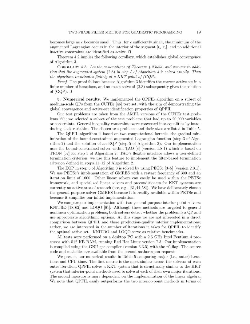
5. Numerical results. We implemented the QPFIL algorithm on a subset ofmedium-scale QPs from the CUTEr [46] test set, with the aim of demonstrating theglobal convergence and active-set identification properties of QPFIL.

Our test problems are taken from the AMPL versions of the CUTEr test prob-lems [60]; we selected a subset of the test problems that had up to 20,000 variablesor constraints. General inequality constraints were converted into equalities by intro-ducing slack variables. The chosen test problems and their sizes are listed in Table 5.

The QPFIL algorithm is based on two computational kernels: the gradual min-imization of the bound-constrained augmented Lagrangian function (step 3 of Algo-rithm 2) and the solution of an EQP (step 5 of Algorithm 3). Our implementationuses the bound-constrained solver within TAO [8] (version 1.8.1) which is based onTRON [52] for step 3 of Algorithm 2. TAO’s flexible interface allows a user-definedtermination criterion; we use this feature to implement the filter-based terminationcriterion defined in steps 11–12 of Algorithm 2.

The EQP in step 5 of Algorithm 3 is solved by using PETSc [3–5] (version 2.3.1).We use PETSc’s implementation of GMRES with a restart frequency of 300 and aniteration limit of 1000. Other linear solvers can easily be used within the PETScframework, and specialized linear solvers and preconditioners for KKT systems arecurrently an active area of research (see, e.g., [31,44,58]). We have deliberately chosenthe general-purpose solver GMRES because it is readily available within PETSc andbecause it simplifies our initial implementation.

We compare our implementation with two general-purpose interior-point solvers:KNITRO [18, 62] and LOQO [61]. Although these methods are targeted to generalnonlinear optimization problems, both solvers detect whether the problem is a QP anduse appropriate algorithmic options. At this stage we are not interested in a directcomparison between QPFIL and these production-quality interior implementations;rather, we are interested in the number of iterations it takes for QPFIL to identifythe optimal active set—KNITRO and LOQO serve as relative benchmarks.

All tests were performed on a desktop PC with a 2.5 GHz Intel Pentium 4 pro-cessor with 512 KB RAM, running Red Hat Linux version 7.3. Our implementationis compiled using the GNU gcc compiler (version 3.3.5) with the -O flag. The sourcecode and makefiles are available from the second author upon request.

We present our numerical results in Table 5 comparing major (i.e., outer) itera-tions and CPU time. The first metric is the most similar across the solvers: at eachouter iteration, QPFIL solves a KKT system that is structurally similar to the KKTsystem that interior-point methods need to solve at each of their own major iterations.The second measure is more dependent on the implementation of the linear algebra.We note that QPFIL easily outperforms the two interior-point methods in terms of


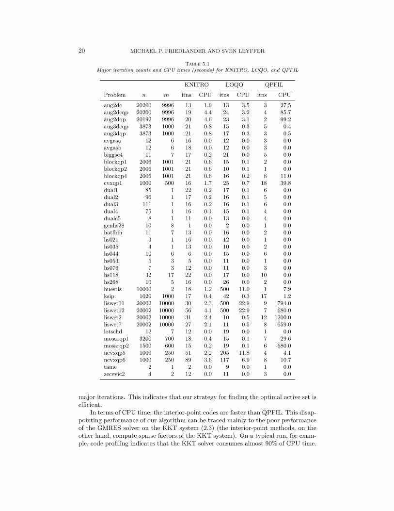
Table 5.1Major iteration counts and CPU times (seconds) for KNITRO, LOQO, and QPFIL

KNITRO LOQO QPFIL

Problem n m itns CPU itns CPU itns CPU

aug2dc 20200 9996 13 1.9 13 3.5 3 27.5aug2dcqp 20200 9996 19 4.4 24 3.2 4 85.7aug2dqp 20192 9996 20 4.6 23 3.1 2 99.2aug3dcqp 3873 1000 21 0.8 15 0.3 5 0.4aug3dqp 3873 1000 21 0.8 17 0.3 3 0.5avgasa 12 6 16 0.0 12 0.0 3 0.0avgasb 12 6 18 0.0 12 0.0 3 0.0biggsc4 11 7 17 0.2 21 0.0 5 0.0blockqp1 2006 1001 21 0.6 15 0.1 2 0.0blockqp2 2006 1001 21 0.6 10 0.1 1 0.0blockqp4 2006 1001 21 0.6 16 0.2 8 11.0cvxqp1 1000 500 16 1.7 25 0.7 18 39.8dual1 85 1 22 0.2 17 0.1 6 0.0dual2 96 1 17 0.2 16 0.1 5 0.0dual3 111 1 16 0.2 16 0.1 6 0.0dual4 75 1 16 0.1 15 0.1 4 0.0dualc5 8 1 11 0.0 13 0.0 4 0.0genhs28 10 8 1 0.0 2 0.0 1 0.0hatfldh 11 7 13 0.0 16 0.0 2 0.0hs021 3 1 16 0.0 12 0.0 1 0.0hs035 4 1 13 0.0 10 0.0 2 0.0hs044 10 6 6 0.0 15 0.0 6 0.0hs053 5 3 5 0.0 11 0.0 1 0.0hs076 7 3 12 0.0 11 0.0 3 0.0hs118 32 17 22 0.0 17 0.0 10 0.0hs268 10 5 16 0.0 26 0.0 2 0.0huestis 10000 2 18 1.2 500 11.0 1 7.9ksip 1020 1000 17 0.4 42 0.3 17 1.2liswet11 20002 10000 30 2.3 500 22.9 9 794.0liswet12 20002 10000 56 4.1 500 22.9 7 680.0liswet2 20002 10000 31 2.4 10 0.5 12 1200.0liswet7 20002 10000 27 2.1 11 0.5 8 559.0lotschd 12 7 12 0.0 19 0.0 1 0.0mosarqp1 3200 700 18 0.4 15 0.1 7 29.6mosarqp2 1500 600 15 0.2 19 0.1 6 680.0ncvxqp5 1000 250 51 2.2 205 11.8 4 4.1ncvxqp6 1000 250 89 3.6 117 6.9 8 10.7tame 2 1 2 0.0 9 0.0 1 0.0zecevic2 4 2 12 0.0 11 0.0 3 0.0

major iterations. This indicates that our strategy for finding the optimal active set isefficient.

In terms of CPU time, the interior-point codes are faster than QPFIL. This disap-pointing performance of our algorithm can be traced mainly to the poor performanceof the GMRES solver on the KKT system (2.3) (the interior-point methods, on theother hand, compute sparse factors of the KKT system). On a typical run, for exam-ple, code profiling indicates that the KKT solver consumes almost 90% of CPU time.


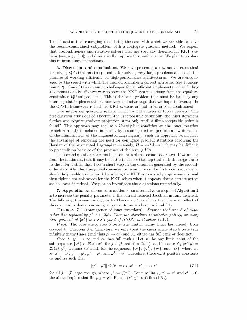
This situation is discouraging considering the ease with which we are able to solvethe bound-constrained subproblem with a conjugate gradient method. We expectthat preconditioners and iterative solvers that are specially designed for KKT sys-tems (see, e.g., [10]) will dramatically improve this performance. We plan to explorethis in future implementations.

6. Discussion and conclusions. We have presented a new active-set methodfor solving QPs that has the potential for solving very large problems and holds thepromise of working efficiently on high-performance architectures. We are encour-aged by the speed with which the method identifies a correct active set (see Proposi-tion 4.2). One of the remaining challenges for an efficient implementation is findinga computationally effective way to solve the KKT systems arising from the equality-constrained QP subproblems. This is the same problem that must be faced by anyinterior-point implementation, however; the advantage that we hope to leverage inthe QPFIL framework is that the KKT systems are not arbitrarily ill-conditioned.

Two interesting questions remain which we will address in future reports. Thefirst question arises out of Theorem 4.2: Is it possible to simplify the inner iterationsfurther and require gradient projection steps only until a filter-acceptable point isfound? This approach may require a Cauchy-like condition on the inner iteration(which currently is included implicitly by assuming that we perform a few iterationsof the minimization of the augmented Lagrangian). Such an approach would havethe advantage of removing the need for conjugate gradient iterations involving theHessian of the augmented Lagrangian—namely, H + ρATA—which may be difficultto precondition because of the presence of the term ρATA.

The second question concerns the usefulness of the second-order step. If we are farfrom the minimum, then it may be better to choose the step that adds the largest areato the filter, rather than take a short step in the direction generated by the second-order step. Also, because global convergence relies only on the first-order sequence, itshould be possible to save work by solving the KKT systems only approximately, andthen tighten the tolerances for the KKT solves when it appears that a correct activeset has been identified. We plan to investigate these questions numerically.

7. Appendix. As discussed in section 3, an alternative to step 6 of Algorithm 2is to increase the penalty parameter if the current reduced Jacobian in rank deficient.The following theorem, analogous to Theorem 3.4, confirms that the main effect ofthis increase is that it encourages iterates to move closer to feasibility.

Theorem 7.1 (convergence of inner iterations). Suppose that step 6 of Algo-rithm 2 is replaced by ρj+1 ← 2ρj. Then the algorithm terminates finitely, or everylimit point x∗ of {xj} is a KKT point of (GQP), or it solves (2.12).

Proof. The case where step 5 tests true finitely many times has already beencovered by Theorem 3.4. Therefore, we only treat the cases where step 5 tests trueinfinitely many times (and thus ρj →∞) and A∗ either has full rank or does not.

Case 1. (ρj → ∞ and A∗ has full rank.) Let x∗ be any limit point of thesub-sequence {xj}J . Each xj , for j ∈ J , satisfies (2.11), and because Lρj (xj , y) =L0(xj , yj), Lemma 3.3 holds for the sequences {xj}, {yj}, {ρj}, and {εj}, where welet xk = xj , yk = yj , ρk = ρj , and ωk = εj . Therefore, there exist positive constantsα1 and α2 such that

‖yj − y∗‖ ≤ βj := α1‖xj − x∗‖+ α2εj (7.1)

for all j ∈ J large enough, where y∗ := y(x∗). Because limj∈J xj = x∗ and εj → 0,

the above implies that limj∈J = y∗. Hence, (x∗, y∗) satisfies (1.3a).


In order to show that x∗ is feasible for (GQP), we use the definition of yj to derive

ρj‖Axj − b‖ = ‖yj − y‖ ≤ ‖yj − y∗‖+ ‖y∗ − y‖ ≤ βj + ‖y∗ − y‖,

where we used the triangle inequality and (7.1). Then εj → 0, limj∈J xj = x∗, and

ρj →∞ imply that Ax∗ = b. Therefore, x∗ satisfies (1.3b), and so (x∗, y∗) is a KKTpoint of (GQP), as required.

Case 2. (ρj → ∞ and A∗ does not have full rank.) The necessary and sufficientoptimality condition for (2.12) is that x∗ satisfy

min{x∗, AT(Ax∗ − b)} = 0. (7.2)

Each xj and zj satisfies (2.11). Therefore,

lim supj∈J

zj ≡ c+Hx∗ −ATy + lim supj∈J

ρjAT(Axj − b) ≥ 0,

which, because ρj →∞, necessarily implies that

z∗ := limj∈J

AT(Axj − b) = AT(Ax∗ − b) ≥ 0. (7.3)

If we consider only the components I∗ of zj , then by (2.11) and εj → 0, (7.3) holdswith equality. But because ρj → ∞ and AT(Ax∗ − b) ≥ 0, we must have thatz∗I = [AT(Ax∗ − b)]I∗ = 0. Therefore, x∗ and z∗ satisfy (7.2).

Acknowledgments. We are grateful to our summer student Anatoly Eydelzon,who developed an initial version of QPFIL using TAO and PETSC, and to Ewoutvan den Berg for his careful reading of this paper. Sincere thanks to Tamara Kolda,and to two anonymous referees, whose many valuable suggestions helped to clarifythe approach and sharpen the theoretical development. In particular, the referees’comments led us to Theorem 3.8 as well as refinements of Algorithm 2.

REFERENCES

[1] R. Andreani, E. G. Birgin, J. M. Martınez, and M. L. Schuverdt, Augmented Lagrangianmethods under the constant positive linear dependence constraint qualification, Math. Pro-gram., (2006).

[2] M. Anitescu, Optimization-based simulation of nonsmooth rigid multibody dynamics, Math.Prog., 105 (2006), pp. 113–143.

[3] S. Balay, K. Buschelman, V. Eijkhout, W. D. Gropp, D. Kaushik, M. G. Knepley, L. C.McInnes, B. F. Smith, and H. Zhang, PETSc Users manual, Tech. Rep. ANL-95/11(Revision 2.1.5), Argonne National Laboratory, 2004.

[4] S. Balay, K. Buschelman, W. D. Gropp, D. Kaushik, M. G. Knepley, L. C. McInnes,B. F. Smith, and H. Zhang, PETSc Web page, 2001. http://www.mcs.anl.gov/petsc.

[5] S. Balay, W. D. Gropp, L. C. McInnes, and B. F. Smith, Efficient management of paral-lelism in object oriented numerical software libraries, in Modern Software Tools in Scien-tific Computing, E. Arge, A. M. Bruaset, and H. P. Langtangen, eds., Birkhauser, 1997,pp. 163–202.

[6] J. L. Barlow and G. Toraldo, The effect of diagonal scaling on projected gradient methodsfor bound constrained quadratic programming problems, Optim. Methods and Softw., 5(1995), pp. 235–245.

[7] G. Bashein and M. Enns, Computation of optimal controls by a method combining quasi-linearization and quadratic programming, Internat. J. Control, 16 (1972), pp. 177–187.

[8] S. J. Benson, L. C. McInnes, J. More, and J. Sarich, TAO user manual (revision 1.8),Tech. Rep. ANL/MCS-TM-242, Mathematics and Computer Science Division, ArgonneNational Laboratory, 2005. http://www.mcs.anl.gov/tao.


[9] S. J. Benson, L. C. McInnes, J. J. More, and J. Sarich, Scalable algorithms in optimiza-tion: Computational experiments, Tech. Rep. ANL/MCS-P1175-0604, Mathematics andComputer Science Division, Argonne National Laboratory, 2004.

[10] M. Benzi, G. Golub, and J. Liesen, Numerical solution of saddle point problems, ActaNumerica, 14 (2005), pp. 1–137.

[11] M. Benzi and G. H. Golub, A preconditioner for generalized saddle point problems, SIAM J.Matrix Anal. Appl., 26 (2004), pp. 20–41.

[12] L. Bergamaschi, J. Gondzio, and G. Zilli, Preconditioning indefinite systems in interiorpoint methods for optimization, Computational Optimization and Applications, 28 (2004),pp. 149–171.

[13] D. P. Bertsekas, Constrained Optimization and Lagrange Multiplier Methods, AcademicPress, New York, 1982.

[14] , Nonlinear Programming, Athena Scientific, Belmont, MA, second ed., 1999.[15] M. J. Best and J. Kale, Quadratic programming for large-scale portfolio optimization, in

Financial Services Information Systems, J. Keyes, ed., CRC Press, 2000, pp. 513–529.[16] G. Biros and O. Ghattas, Parallel Lagrange–Newton–Krylov–Schur methods for PDE-

constrained optimization. Part I: The Krylov–Schur solver, SIAM J. Sci. Comput., 27(2005), pp. 687–713.

[17] R. H. Byrd, N. I. M. Gould, J. Nocedal, and R. A. Waltz, An algorithm for nonlinear op-timization using linear programming and equality constrained subproblems, MathematicalProgramming, Series B, 100 (2004), pp. 27–48.

[18] R. H. Byrd, J. Nocedal, and R. A. Waltz, Knitro: An integrated package for nonlinear op-timization, in Large-Scale Nonlinear Optimization, G. di Pillo and M. Roma, eds., SpringerVerlag, 2006, pp. 35–59.

[19] C. Chin and R. Fletcher, On the global convergence of an SLP-filter algorithm that takesEQP steps, Math. Prog., 96 (2003), pp. 161–177.

[20] T. F. Coleman and Y. Li, A reflective Newton method for minimizing a quadratic functionsubject to bounds on some of the variables, SIAM J. Optim., 6 (1996), pp. 1040–1058.

[21] A. R. Conn, N. I. M. Gould, and Ph. L. Toint, Testing a class of methods for solvingminimization problems with simple bounds on the variables, Math. Comp., 50 (1988),pp. 399–430.

[22] A. R. Conn, N. I. M. Gould, and P. L. Toint, LANCELOT: A Fortran package for large-scale nonlinear optimization (Release A), Springer Verlag, Heidelberg, 1992.

[23] A. R. Conn, N. I. M. Gould, and Ph. L. Toint, A globally convergent augmented Lagrangianalgorithm for optimization with general constraints and simple bounds, SIAM J. Numer.Anal., 28 (1991), pp. 545–572.

[24] F. Delbos and J. Gilbert, Global linear convergence of an augmented lagrangian algorithmfor solving convex quadratic optimization problems, J. Convex Anal., 12 (2005), pp. 45–69.

[25] M. A. Diniz-Ehrhardt, M. A. Gomes-Ruggiero, and S. A. Santos, Numerical analysisof leaving-face parameters in bound-constrained quadratic minimization, Optim. MethodsSoftw., 15 (2001), pp. 45–66.

[26] Z. Dostal, Box constrained quadratic programming with controlled precision of auxiliary prob-lems and applications, Z. Angew. Math. Mech., 76 (1996), pp. 413–414.

[27] , Box constrained quadratic programming with proportioning and projections, SIAM J.Optim., 7 (1997), pp. 871–887.

[28] Z. Dostal, A. Friedlander, and S. A. Santos, Adaptive precision control in quadraticprogramming with simple bounds and/or equality constraints, in High Performance Algo-rithms and Software in Nonlinear Optimization, R. D. Leone, A. Murli, P. M. Pardalos,and G. Toraldo, eds., Dordrecht, The Netherlands, 1998, Kluwer Academic Publishers,pp. 161–173.

[29] , Augmented Lagrangians with adaptive precision control for quadratic programming withequality constraints, Comput. Optim. Appl., 14 (1999), pp. 37–53.

[30] , Augmented Lagrangians with adaptive precision control for quadratic programming withsimple bounds and equality constraints, SIAM J. Optim., 13 (2003), pp. 1120–1140.

[31] I. S. Duff, MA57—a code for the solution of sparse symmetric definite and indefinite systems,ACM Trans. Math. Softw., 30 (2004), pp. 118–144.

[32] K. A. Fegley, S. Blum, J. O. Bergholm, A. J. Calise, J. E. Marowitz, G. Porcelli,and L. P. Sinha, Stochastic and deterministic design and control via linear and quadraticprogramming, IEEE Trans. Automat. Control, AC-16 (1971), pp. 759–766.

[33] R. Fletcher, A general quadratic programming algorithm, J. Inst. Math. Appl., 7 (1971),pp. 76–91.

[34] , Resolving degeneracy in quadratic programming, Ann. Oper. Res., 47 (1993), pp. 307–


334.[35] R. Fletcher and E. S. de la Maza, Nonlinear Programming and nonsmooth Optimization

by successive Linear Programming, Math. Prog., 43 (1989), pp. 235–256.[36] R. Fletcher and S. Leyffer, Nonlinear programming without a penalty function, Math.

Prog., 91 (2002), pp. 239–269.[37] A. Forsgren, Inertia-controlling factorizations for optimization algorithms, Appl. Numer.

Math., 43 (2002), pp. 91–107.[38] A. Forsgren, P. E. Gill, and M. H. Wright, Interior methods for nonlinear optimization,

SIAM Rev., 44 (2002), pp. 525–597.[39] A. Friedlander and J. M. Martınez, On the maximization of a concave quadratic function

with box constraints, SIAM J. Optim., 4 (1994), pp. 177–192.[40] M. P. Friedlander and M. A. Saunders, A globally convergent linearly constrained La-

grangian method for nonlinear optimization, SIAM J. Optim., 15 (2005), pp. 863–897.[41] P. E. Gill, W. Murray, D. B. Ponceleon, and M. A. Saunders, Preconditioners for indefi-

nite systems arising in optimization, SIAM J. Matrix Anal. Appl., 13 (1992), pp. 292–311.[42] P. E. Gill, W. Murray, and M. A. Saunders, User’s guide for SQOPT 5.3: A Fortran

package for large-scale linear and quadratic programming, Tech. Rep. NA 97-4, Departmentof Mathematics, University of California, San Diego, 1997.

[43] P. E. Gill, W. Murray, M. A. Saunders, and M. H. Wright, Inertia-controlling methodsfor general quadratic programming, SIAM Rev., 33 (1991), pp. 1–36.

[44] G. H. Golub, C. Greif, and J. M. Varah, An algebraic analysis of a block diagonal precon-ditioner for saddle point systems, SIAM J. Matrix Anal. Appl., 27 (2006), pp. 779–792.

[45] N. I. M. Gould, S. Leyffer, and P. L. Toint, A multidimensional filter algorithm fornonlinear equations and nonlinear least squares, SIAM J. Optim., 15 (2004), pp. 17–38.

[46] N. I. M. Gould, D. Orban, and Ph. L. Toint, CUTEr and SifDec: A constrained and uncon-strained testing environment, revisited, ACM Trans. Math. Software, 29 (2003), pp. 373–394.

[47] N. I. M. Gould and P. L. Toint, SQP methods for large-scale nonlinear programming, inSystem Modelling and Optimization, Methods, Theory and Applications, M. J. D. Powelland S. Scholtes, eds., Kluwer Academic Publishers, 2000, pp. 149–178.

[48] N. I. M. Gould and P. L. Toint, An iterative working-set method for large-scale non-convexquadratic programming, Tech. Rep. RAL-TR-2001–026, Rutherford Appleton Laboratory,Chilton, Oxfordshire, England, 2001.

[49] , Numerical methods for large-scale non-convex quadratic programming, in Trends inIndustrial and Applied Mathematics, A. H. Siddiqi and M. Kocvara, eds., Kluwer AcademicPublishers, 2002, pp. 149–179.

[50] G. D. Hart and M. Anitescu, A hard-constraint time-stepping approach for rigid multibodydynamics with joints, contact, and friction, in Proceedings of the ACM 2003 Tapia Con-ference for Diversity in Computing, Atlanta, GA, 2003, pp. 34–40.

[51] R. M. Larsen, Combining implicit restart and partial reorthogonalization in Lanczos bidiag-nalization, 2001. http://sun.stanford.edu/~rmunk/PROPACK/.

[52] C.-J. Lin and J. J. More, Newton’s method for large bound-constrained optimization problems,SIAM J. Optim., 9 (1999), pp. 1100–1127.

[53] K. Malanowski, On application of a quadratic programming procedure to optimal control prob-lems in systems described by parabolic equations, Control and Cybern., 1 (1972), pp. 43–56.

[54] H. M. Markowitz, The optimization of a quadratic function subject to constraints, Nav. Res.Logist. Q., 3 (1956), pp. 111–133.

[55] J. J. More and G. Toraldo, On the solution of quadratic programming problems with boundconstraints, SIAM J. Optim., 1 (1991), pp. 93–113.

[56] Y. E. Nesterov and A. Nemirovski, Interior-point polynomial methods in convex program-ming, vol. 14 of Stud. Appl. Math., SIAM, Philadelphia, 1994.

[57] J. Nocedal and S. Wright, Numerical Optimization, Springer Verlag, Berlin, 1999.[58] O. Schenk and K. Gartner, Solving unsymmetric sparse systems of linear equations with

PARDISO, Future Generation Computer Systems, 20 (2004), pp. 475–487.[59] M. Ulbrich, S. Ulbrich, and L. Vicente, A globally convergent primal-dual interior-point

filter method for nonlinear programming, Math. Prog., 100 (2004), pp. 379–410.[60] R. Vanderbei, Benchmarks for nonlinear optimization, December 2002. http://www.

princeton.edu/~rvdb/bench.html.[61] R. Vanderbei and D. Shanno, An interior point algorithm for nonconvex nonlinear program-

ming, COAP, 13 (1999), pp. 231–252.[62] R. A. Waltz and T. D. Plantenga, KNITRO 5.0 User’s Manual, Ziena Optimization, Inc.,

Evanston, IL, Feb. 2006.

global and finite termination of a two-phase …

Documents