global attractivity of equilibrium in gierer–meinhardt system with activator production saturation...

Nonlinear Analysis: Real World Applications 14 (2013) 1871–1886

Contents lists available at SciVerse ScienceDirect

Nonlinear Analysis: Real World Applications

journal homepage: www.elsevier.com/locate/nonrwa

Global attractivity of equilibrium in Gierer–Meinhardtsystem with activator production saturation and geneexpression time delays

Shanshan Chen a, Junping Shi b,∗a Department of Mathematics, Harbin Institute of Technology, Weihai, Shandong, 264209, PR Chinab Department of Mathematics, College of William and Mary, Williamsburg, VA, 23187-8795, USA

a r t i c l e i n f o

Article history:Received 23 February 2012Accepted 20 December 2012

Keywords:Gierer–Meinhardt systemTime delaysGene expressionGlobal attractivity

a b s t r a c t

In thisworkwe investigate a diffusive Gierer–Meinhardt systemwith gene expression timedelays in the production of activators and inhibitors, and also a saturation in the activatorproduction, which was proposed by Seirin Lee et al. (2010) [10]. We rigorously considerthe basic kinetic dynamics of the Gierer–Meinhardt system with saturation. By using anupper and lower solution method, we show that when the saturation effect is strong, theunique constant steady state solution is globally attractive despite the time delays. Thisresult limits the parameter space for which spatiotemporal pattern formation is possible.

© 2013 Elsevier Ltd. All rights reserved.

1. Introduction

Since the pioneering work of Turing [1], Reaction–Diffusion systems have been used to demonstrate morphogeneticpattern formation [2–7]. During the process of cell division and differentiation, gene expressions control the establishmentof stable patterns of differentiated cell types. Recent experimental studies have shown that timing of the pattern-formingevents may have important implications in the development of the patterns [8,9,4,5,10,11]. In particular, there existsa considerable delay between the start of protein signal transduction (ligand–receptor binding) and the result (a geneproduction) via gene expression regulations [10].

In 1972, Gierer and Meinhardt [12] proposed a nonlinear reaction–diffusion model to describe the interaction dynamicsof two chemical substances: (see [12, Eq. (12)])

∂a∂t

= ρ0ℓa + cℓaap

hq− νaa + Da

∂2a∂x2

,

∂h∂t

= c ′ℓhar

hs− νhh + Dh

∂2h∂x2

,

(1.1)

where a(x, t) and h(x, t) are the concentrations of the activator and the inhibitor respectively; the reactions of activators andinhibitors are assumed to be power functions of a and h, and at the same time both substances are removed at a linear rate;the activator a and the inhibitor hdiffuse in the environmentwith diffusion constantDa andDh respectively, and it is assumedthat h diffuses faster than a; finally a constant source term for a initiates the whole reaction. Here ℓa, ρ0, ℓh, c, νa, c ′, νh areall positive constant parameters, and the exponents p, q, r, s are all nonnegative. One of particular examples of exponents

Partially supported by a grant from China Scholarship Council, NSF grant DMS-1022648, and Shanxi 100-talent program.∗ Corresponding author. Tel.: +1 757 221 2030.

E-mail addresses: [email protected], [email protected] (J. Shi).

1468-1218/$ – see front matter© 2013 Elsevier Ltd. All rights reserved.doi:10.1016/j.nonrwa.2012.12.004

http://dx.doi.org/10.1016/j.nonrwa.2012.12.004

http://www.elsevier.com/locate/nonrwa

http://www.elsevier.com/locate/nonrwa

http://crossmark.dyndns.org/dialog/?doi=10.1016/j.nonrwa.2012.12.004&domain=pdf

mailto:[email protected]

mailto:[email protected]

http://dx.doi.org/10.1016/j.nonrwa.2012.12.004

1872 S. Chen, J. Shi / Nonlinear Analysis: Real World Applications 14 (2013) 1871–1886

they considered was q = 1, s = 0, and p = r = 2. That is, two molecules of activator are necessary to activate, and onemolecule of inhibitor is needed for inhibit; and the activators activate both substances and the inhibitors only inhibit theactivator source.

On the other hand, by assuming a saturation of activator production for the case q = 1, s = 0, and p = r = 2 in (1.1),Gierer and Meinhardt [12] also considered (see [12, Eq. (16)])

∂a∂t

= ρ0ℓa + cℓaa2

(1 + κa2)h− νaa + Da

∂2a∂x2

,

∂h∂t

= c ′ℓha2 − νhh + Dh∂2h∂x2

.

(1.2)

For system (1.2), the activator concentration is limited to amaximumvalue so that the activated area forms an approximatelyconstant proportion of the total structure size. Numerical simulation of concentration patterns were obtained in [12] as wellas [13,14] for one and two-dimensional spatial domains.

Since then, the Gierer–Meinhardt system has been regarded as one of the prototype reaction–diffusion models ofspatiotemporal pattern formation [15,16], and extensive research has been done for a more general Gierer–Meinhardtsystem in the form of (with κ = 0 or κ > 0)

∂u∂t

= ϵ21u − u + ρaup

(1 + κup)vq+ σa, x ∈ Ω, t > 0,

τ∂v

∂t= D1v − v + ρh

ur

vs+ σh, x ∈ Ω, t > 0,

∂u(x, t)∂ν

=∂v(x, t)

∂ν= 0, x ∈ ∂Ω, t > 0,

u(x, 0) = u0(x) > 0, v(x, 0) = v0(x) > 0, x ∈ Ω.

(1.3)

Here, Ω is a bounded smooth region in Rn, n ≥ 1 and the Laplace operator 1w(x, t) =n

i=1∂2w(x,t)

∂x2ifor w = u, v

shows the diffusion effect; ∂w(x,t)∂ν

is the outer normal derivative of w = u, v, and a no-flux boundary condition isimposed; the coefficients ϵ, τ and D are positive constants, whereas κ is a nonnegative constant; the basic production termsσa = σa(x), σh = σh(x) are nonnegative, and the interaction coefficients ρa = ρa(x), ρh = ρh(x) are positive over Ω . Upto now, there are many research results on the nonhomogeneous steady state solutions (such as multi-peak steady statesolutions, etc.) of the Gierer–Meinhardt system (1.1), (see Refs. [17–25]) and the Gierer–Meinhardt system with saturation(1.2), (see Refs. [26–29]), and the a priori estimates, global existence and asymptotic behavior of the solution [30–35].

In this paperwe assume that σa, ρa and ρh are positive constants, the basic production term σh(x) ≡ 0, and the saturationparameter κ is a positive constant. Then system (1.3) becomes:

∂u∂t

= ϵ21u − u + ρaup

(1 + κup)vq+ σa, x ∈ Ω, t > 0,

τ∂v

∂t= D1v − v + ρh

ur

vs, x ∈ Ω, t > 0,

∂u(x, t)∂ν

=∂v(x, t)

∂ν= 0, x ∈ ∂Ω, t > 0,

u(x, 0) = u0(x) > 0, v(x, 0) = v0(x) > 0, x ∈ Ω

(1.4)

where ρa, κ, σa, ρh, ϵ, τ and D are positive constants. We show that when the saturation constant κ is large then theunique constant steady state solution is globally attractive, hence no spatiotemporal pattern is possible. In [28] assumingp = r = 2, s = 0 and q = 1, Morimoto showed that system (1.4) admits a radially symmetric steady state solution whenκ is small, and the global stability proved here implies that (1.4) cannot have such radially symmetric steady state solutionwhen κ is large.

In recent studies Gaffney and Monk [8] and Seirin Lee et al. [10] (see also [36,37]) considered the effect of geneexpression time delays on morphogenesis and pattern formation. The time delays in the feedback can be caused by thesignal transduction, gene transcription and mRNA translation in the process of gene expression [10]. Here we consider theGierer–Meinhardt system with gene expression time delays and saturation of activator induced activator production asproposed in [10] (model I with saturation of activator induced activator production in [10]):

∂u∂t

= D1∂2u∂x2

+ k1 − k2u(x, t) + k3u2(x, t − γ )

(1 + κu2(x, t − γ ))v(x, t − γ ),

∂v

∂t= D2

∂2v

∂x2+ k4u2(x, t − γ ) − k5v(x, t),

(1.5)

S. Chen, J. Shi / Nonlinear Analysis: Real World Applications 14 (2013) 1871–1886 1873

where u, v are the concentrations of the activator and the inhibitor respectively; ki (1 ≤ i ≤ 5) are positive and indicatethe production rate, the decay rates and the rate of gene product interaction of morphogens, κ ≥ 0 represents the effect ofthe saturation, and γ ≥ 0 is the gene expression time delay in the morphogen induced protein production.

Indeed we consider a generalized nonlocal Gierer–Meinhardt system with gene expression time delays:

∂u∂t

= ϵ21u − u + ρa

Ω

k1(x, y)up(y, t − γ )

(1 + κup(y, t − γ ))vq(y, t − γ )dy + σa, x ∈ Ω, t > 0,

τ∂v

∂t= D1v − v + ρh

Ω

k2(x, y)ur(y, t − γ )dy x ∈ Ω, t > 0,

∂u(x, t)∂ν

=∂v(x, t)

∂ν= 0, x ∈ ∂Ω, t > 0,

u(x, t) = u0(x, t) > 0, v(x, t) = v0(x, t) > 0, x ∈ Ω, t ∈ [−γ , 0],

(1.6)

following the general version in Suzuki and Takagi [34]. And the dispersal kernel functions ki(x, y), (i = 1, 2), satisfy thefollowing property (see, for example [38,39]):

(K ) Either ki(x, y) = δ(x − y) (Dirac Delta function), or ki(x, y) is a continuous and nonnegative function such thatΩki(x, y)dy = 1 for any x ∈ Ω and the linear operator

Li(φ)(x) :=

Ω

ki(x, y)φ(y)dy

is strictly positive on C(Ω, R) in the sense that

Li(C(Ω, R+) \ 0) ⊂ C(Ω, R+) \ 0.

The generalization of (1.5) to a nonlocal model as in (1.6) is motivated by recent work in [40,41,38,42], as the effects ofdiffusion and time delays are not independent of each other, and the individuals have not been at the same point in space atprevious time. Hence a spatial averaging of the population in the past time should be added to take account of that effect inthe models, and a detailed review on that topic can be found in Gourley, So and Wu [42]. Such formulation for the modelsin a bounded domain first appeared in Gourley and So [38], and see also [40,41,43,39]. In Section 4, we will also commenton the validity of assumption (K ).

Note that when ki(x, y) = δ(x − y), (i = 1, 2), system (1.6) reduces to the following time-delayed reaction–diffusionsystem (as in [10]):

∂u∂t

= ϵ21u − u + ρaup(x, t − γ )

(1 + κup(x, t − γ ))vq(x, t − γ )+ σa, x ∈ Ω, t > 0,

τ∂v

∂t= D1v − v + ρhur(x, t − γ ) x ∈ Ω, t > 0,

∂u(x, t)∂ν

=∂v(x, t)

∂ν= 0, x ∈ ∂Ω, t > 0,

u(x, t) = u0(x, t) > 0, v(x, t) = v0(x, t) > 0, x ∈ Ω, t ∈ [−γ , 0].

(1.7)

Again our main result is that the unique constant steady state solution is globally asymptotically stable when the saturationconstant κ is large, but the result for the delayed system (1.6) is that the exponent s in system (1.4) is 0 in (1.6). Whilethis shows the restriction of the mathematical method of proving the global stability, it may suggest that the additionalfeedback of vs term in (1.4) could enrich the dynamics. We use a upper–lower solution method for the proof of globalstability, which was developed by Pao [44–47], and see also related work in [48,49]. We remark that the global stabilityof constant equilibrium in a scalar delayed reaction–diffusion equation have also been proved by using dynamical systemapproach [50,51], Lyapunov method [52,53], and fluctuation method [43,39].

Our analysis here shows that a strong saturation effect plays a role of stabilizing the constant steady state even when thedelays exist. That is, when κ is sufficiently large, the constant steady state is globally stable and no complex spatiotemporalpatterns appear despite gene expression delays. This shows that in the delayed Gierer–Meinhardt system with saturation,the degree of saturation is the most important parameter for the dynamics, while the time-delay is a secondary parameterwhich can be the determining factor in the small saturation case. This is one step to rigorously analyze the dynamicalbehavior of this prototype biological pattern formation system. Another step is to analyze the bifurcation of the systemusingthe time-delay as bifurcation parameter when κ is small, which has been reported in [10]. The instability of the constantequilibrium for a small κ but a large delay has been rigorously proved in our other work [54]. Hence the present workcomplements the one in [54,10].

The rest of this paper is organized as follows. In Section 2, we present some preliminaries: in Section 2.1, the basicdynamics of the kinetic model is presented; and in Section 2.2, we recall the comparison method of the reaction–diffusionsystemswith delay effect. In Section 3, we prove the global stability of the unique constant steady state solutionwith respectto the reaction–diffusion system without the delay effect (1.4). In Section 4, we prove the global stability of the unique


constant steady state solution with respect to the reaction–diffusion system with gene expression time delays (1.6) for anydelay γ > 0. Section 5 contains some concluding remarks. Throughout the paper, (a, b) > 0 means a > 0 and b > 0 for(a, b) ∈ R2.

2. Preliminaries

2.1. Analysis of the kinetic system

In this subsection, we analyze the following kinetic system corresponding to system (1.4):dudt

= −u + ρaup

(1 + κup)vq+ σa, t > 0,

τdvdt

= −v + ρhur

vs, t > 0,

u(0) = u0 > 0, v(0) = v0 > 0.

(2.1)

In this subsection, we always assume that ρa, ρh, σa, τ , p, q, r > 0, and s, κ ≥ 0.

Lemma 2.1. Suppose that the parameters ρa, ρh, σa, τ , p, q, r > 0, and s, κ ≥ 0. If

p − 1r

<q

s + 1, (2.2)

then system (2.1) has a unique positive constant equilibrium (u∗, v∗), where v∗ = (ρhur∗)

1s+1 .

Proof. If (u, v) is an equilibrium of system (2.1), then (u, v) satisfies

−u + ρaup

(1 + κup)vq+ σa = 0, −v + ρh

ur

vs= 0,

which implies u satisfies

1 + κup= ρaρ

−q

s+1h

up− qrs+1

u − σa. (2.3)

Define

I1(u) := ρaρ−

qs+1

hup− qr

s+1

u − σa,

and it can be easily verified that I1(u) is a strictly decreasing function foru > σa if (2.2) is satisfied.Moreover limu→σ+aI1(u) =

∞, limu→∞ I1(u) = 0 if (2.2) is satisfied. On the other hand, the function I2(u) := 1 + κup satisfies I2(0) = 1 and it isincreasing on (0, ∞). Hence if (2.2) is satisfied, then the system has a unique positive constant equilibrium (u∗, v∗), whereu∗ is the unique positive root of (2.3), and v∗ = (ρhur

∗)

1s+1 .

From the proof of Lemma 2.1, we define β > σa to be the unique point such that I1(β) = 1. That is, β is the unique pointsatisfying

ρ−1a ρ

qs+1h (β − σa) = βp− qr

s+1 . (2.4)

For fixed parameters ρa, σa, ρh, p, q, r, s, we regard u∗ as a function of κ and u∗(0) = β . Then one can show that u∗(κ) isstrictly decreasing in κ . Indeed by differentiating 1 + κup

∗(κ) = I1(u∗(κ)), and using that I ′1(u) < 0 for u > σa, we seethat u′

∗(κ) < 0. Since 1 + κup

∗(κ) = I1(u∗(κ)), we have I1(u∗(κ)) → ∞ as κ → ∞. Hence limκ→∞ u∗(κ) = σa andlimκ→0+ u∗(κ) = β .

We can now arrive at the following result about the local stability of the equilibrium (u∗, v∗).

Theorem 2.2. Suppose that the parameters ρa, ρh, σa, τ , p, q, r > 0, s, κ ≥ 0, β is defined as in Eq. (2.4), and p/r ≤ q/(s+1).

1. If

β − σa

β<

1p

1 +

s + 1τ

, (2.5)

then (u∗, v∗) is locally asymptotically stable for any κ ≥ 0.


2. If

β − σa

β≥

1p

1 +

s + 1τ

, (2.6)

then there exists κ ≥ 0 such that(i) if κ > κ , then (u∗, v∗) is locally asymptotically stable;(ii) if κ < κ , then (u∗, v∗) is unstable;(iii) system (2.1) undergoes a Hopf bifurcation when κ = κ at the positive equilibrium (u∗, v∗), and (2.1) possesses at least

one periodic orbit for any κ < κ;(iv) if β−σa

β=

1p

1 +

s+1τ

, then κ = 0.

Proof. Since the Jacobian matrix at the positive equilibrium (u∗, v∗) is−1 + ρa

pup−1∗

(1 + κup∗)2v

q∗

−qρaup

∗

1 + κup∗

v−q−1∗

rρh

τ

ur−1∗

vs∗

−s + 1

τ

,

using Eq. (2.3) and v∗ = (ρhur∗)

1s+1 , we can calculate the determent of Jacobian matrix to be

D(u∗) =1τ

s + 1 + ρaρ−

qs+1

hup−1− qr

s+1∗

1 + κup∗

−

p(s + 1)1 + κup

∗

+ qr ,

and the trace of Jacobian matrix is

T (u∗) = −

1 +

s + 1τ

+ ρ−1

a ρq

s+1h pu

−p−1+ qrs+1

∗ (u∗ − σa)2.

Since p/r ≤ q/(s + 1), we see that for any σa < u∗ ≤ β , D(u∗) > 0 and T ′(u) > 0 for u > σa. If (2.5) is satisfied, thenT (β) < 0. Hence for any σa < u∗ < β, T (u∗) < 0, which implies that (u∗, v∗) is locally asymptotically stable for any κ ≥ 0if (2.5) is satisfied.

On the other hand, if (2.6) is satisfied, by using T ′(u) > 0 and T (σa) < 0, then we see that there exists a unique u∗ suchthat T (u∗) > 0 for u∗ > u∗, T (u∗) < 0 for u∗ < u∗, and T (u∗) = 0. Since u∗(κ) is strictly decreasing in κ , there exists κ ≥ 0such that when κ > κ , then (u∗, v∗) is locally asymptotically stable; when κ < κ , then (u∗, v∗) is unstable, and

dT (u(κ))

dκ

κ=κ

=dT (u)du

u=u(κ)

·du(κ)

dκ

κ=κ

< 0.

System (2.1) undergoes a Hopf bifurcation at the positive equilibrium (u∗, v∗) for κ = κ , and from Poincáre–Bendixsontheory, system (2.1) possesses a periodic orbit when κ < κ . It is easy to verify that if β−σa

β=

1p

1 +

s+1τ

, then κ = 0.

Remark 2.3. We notice that β is a numerical value which depends on all other parameters except κ and τ , and in general βcannot be explicitly solved. Also the condition p/r ≤ q/(s+1) in Theorem 2.2 is more restrictive than (p−1)/r < q/(s+1)in Lemma 2.1. But for the special case p = r = 2, s = 0 and q = 1 as in (1.2), one can directly calculate β = σa + ρaρ

−1h

and β−σaβa

=ρaρ

−1h

σa+ρaρ−1h

in Theorem 2.2. We choose σa = 0.5, ρa = 1, ρh = 1, and τ = 4, then in this case we have that

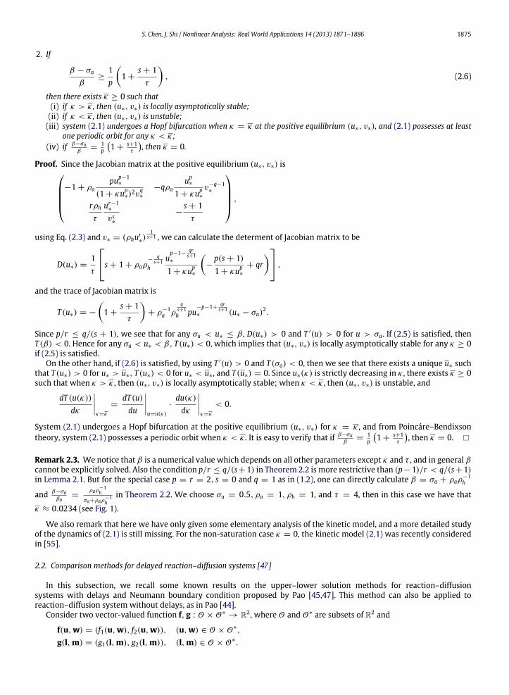
κ ≈ 0.0234 (see Fig. 1).

We also remark that here we have only given some elementary analysis of the kinetic model, and a more detailed studyof the dynamics of (2.1) is still missing. For the non-saturation case κ = 0, the kinetic model (2.1) was recently consideredin [55].

2.2. Comparison methods for delayed reaction–diffusion systems [47]

In this subsection, we recall some known results on the upper–lower solution methods for reaction–diffusionsystems with delays and Neumann boundary condition proposed by Pao [45,47]. This method can also be applied toreaction–diffusion system without delays, as in Pao [44].

Consider two vector-valued function f, g : O × O∗→ R2, where O and O∗ are subsets of R2 and

f(u,w) = (f1(u,w), f2(u,w)), (u,w) ∈ O × O∗,

g(l,m) = (g1(l,m), g2(l,m)), (l,m) ∈ O × O∗.


Fig. 1. Hopf bifurcation diagramwith parameter κ . Here p = r = 2, s = 0, q = 1, σa = 0.5, ρa = 1, ρh = 1. The horizontal axis is κ , the vertical axis is u,and the vertical lines represent the u-range of the periodic orbits. Here a family of limit cycles bifurcate from the Hopf point κ ≈ 0.0234 and the directionof the Hopf bifurcation is backward and supercritical. The diagram is plotted using Matcont.

By writing the vector u,w, l and m in the split form

u ≡ (ui, [u]ai , [u]bi), w ≡ ([w]ei , [w]di), l ≡ ([l]αi , [l]βi), m ≡ ([m]γi , [m]δi)

where [v]σ denotes a vector with σ number of components of v for v = u,w, l or m, the function f(u,w) is said to bequasimonotone in O × O∗ if for any i = 1, 2, there exist nonnegative integers ai, bi, ei and di satisfying the relations

ai + bi = 1, ei + di = 2 (2.7)

such that the function

fi(u,w) ≡ fi(ui, [u]ai , [u]bi , [w]ei , [w]di)

is nondecreasing in each component of [u]ai and [w]ei , and is nonincreasing in each component of [u]bi and [w]di . Similarly,the function g(l,m) is said to be quasimonotone in O × O∗ if for any i = 1, 2, there exist nonnegative integers αi, βi, γi andδi satisfying the relations

αi + βi = 2, γi + δi = 2 (2.8)

such that the function

gi(l,m) ≡ gi([l]αi , [l]βi , [m]γi , [m]δi)

is nondecreasing in each component of [l]αi and [m]γi , and is nonincreasing in each component of [l]βi and [m]δi .We consider the following general reaction–diffusion system with delay and nonlocal effect:

∂u1

∂t= D11u1 + f1(u1(x, t), u2(x, t), u1(x, t − γ ), u2(x, t − γ ))

+

Ω

k1(x, y)g1(u1(y, t), u2(y, t), u1(y, t − γ ), u2(y, t − γ ))dy, x ∈ Ω, t > 0,

∂u2

∂t= D21u2 + f2(u1(x, t), u2(x, t), u1(x, t − γ ), u2(x, t − γ ))

+

Ω

k2(x, y)g2(u1(y, t), u2(y, t), u1(y, t − γ ), u2(y, t − γ ))dy, x ∈ Ω, t > 0,

∂u1(x, t)∂ν

=∂u2(x, t)

∂ν= 0, x ∈ ∂Ω, t > 0,

u1(x, t) = φ1(x, t) ≥ 0, u2(x, t) = φ2(x, t) ≥ 0, x ∈ Ω, t ∈ [−γ , 0],

(2.9)

where the kernel functions k1(x, y) and k2(x, y) satisfy the second assumption in (K). If ki is the Delta function in (1.6), thenwe can simply assume ki ≡ 0 in (2.9). Suppose that there exist two vectors c and c in R2 such that c ≤ c and for i = 1, 2,

fi(c i, [c]ai , [c]bi , [c]ei , [c]di) + gi([c]αi , [c]βi , [c]γi , [c]δi) ≤ 0,fi(c i, [c]ai , [c]bi , [c]ei , [c]di) + gi([c]αi , [c]βi , [c]γi , [c]δi) ≥ 0;

(2.10)


f(u,w) and g(l,m) are quasimonotone in a subset ⟨c, c⟩ × ⟨c, c⟩ where ⟨c, c⟩ = c ∈ R2: c ≤ c ≤ c, and for each

i = 1, 2, fi(u,w) and gi(l,m) satisfy the Lipschitz conditionfi(u,w) − fi(u′,w′) ≤ Ki(

u − u′+ w − w′

),gi(l,m) − gi(l′,m′) ≤ Ki(

l − l′+ m − m′

) (2.11)

for (u,w), (u′,w′), (l,m) and (l′,m′) in ⟨c, c⟩×⟨c, c⟩ and some Ki > 0. Following [47] we define two sequences of constantvectors cm = (cm1 , cm2 ), cm = (cm1 , cm2 ), from the recursion relations

cmi = cm−1i +

1Ki

fi(cm−1i , [cm−1

]ai , [cm−1

]bi , [cm−1

]ei , [cm−1

]di),

+1Ki

gi([cm−1]αi , [c

m−1]βi , [c

m−1]γi , [c

m−1]δi),

cmi = cm−1i +

1Ki

fi(cm−1i , [cm−1

]ai , [cm−1

]bi , [cm−1

]ei , [cm−1

]di),

+1Ki

gi([cm−1]αi , [c

m−1]βi , [c

m−1]γi , [c

m−1]δi),

(2.12)

for m = 1, 2, . . . , i = 1, 2 and c0 = c, c0 = c. From [47, Lemma 2.1] and [45], the sequences cm and cm satisfy themonotonicity property

c ≤ cm ≤ cm+1≤ cm+1

≤ cm ≤ c, m = 1, 2, . . . . (2.13)Hence there exist limits c and c such that limm→∞ cm = c and limm→∞ cm = c. From [47, Theorem 2.2], [47, Corollary 2.1]and [45], the asymptotical dynamics of the reaction–diffusion system with delays (2.9) can be obtained as follows:

Theorem 2.4 ([47]). Suppose there exist c ≤ c satisfying (2.10), f(u,w) and g(l,m) are quasimonotone and satisfy (2.11) in⟨c, c⟩ × ⟨c, c⟩. Then for any initial condition φ = (φ1, φ2) in ⟨c, c⟩, the solution u(x, t) = (u1(x, t), u2(x, t)) ofsystem (2.9) satisfies the relation

c ≤ u(x, t) ≤ c, t ∈ (0, ∞), x ∈ Ω. (2.14)

If, in addition, c = c = c∗, then c∗ is the unique steady state solution of system (2.9) in ⟨c, c⟩ and

limt→∞

u(x, t) = c∗, uniformly for x ∈ Ω. (2.15)

Corollary 2.5 ([47]). Let the conditions in Theorem 2.4 hold, and let

u(x, t) = (u1(x, t), u2(x, t))

be the solution of system (2.9) of an arbitrary initial function φ. If there exists t∗ > 0 such that

c ≤ u(x, t) ≤ c, for t∗ − τ ≤ t ≤ t∗, x ∈ Ω,

then u(x, t) satisfies (2.14) for all t > t∗. Moreover if c = c, then (2.15) holds.

Remark 2.6. For reaction–diffusion systemswithout delays, f(u,w) = f(u). And since f is independent ofw, then the choiceof ei and di does not affect the equation. The general theory of upper–lower solutions of such systems have been consideredin pp. 424–431 of [44], for example.

Remark 2.7. 1. For system (1.4) without delays, g(l,m) = 0, and f(u) = (f1(u), f2(u)), where

f1(u) = −u + ρaup

(1 + κup)vq+ σa,

f2(u) =1τ

−v + ρh

ur

vs

,

and u = (u, v). Here a1 = 0, b1 = 1, a2 = 1, b2 = 0, [u]b1 = v and [u]a2 = u. In this case, the nonlinearity (f1, f2) iscalled mixed quasimonotone as one of ai and one of bi are not zero. Hence the coupled upper solution (c1, c2) and lowersolution (c1, c2) of system (1.4) satisfy

0 ≥ σa − c1 + ρacp1

(1 + κcp1)cq2, 0 ≥ ρh

cr1cs2

− c2,

0 ≤ σa − c1 + ρacp1

(1 + κcp1)cq2, 0 ≤ ρh

cr1cs2

− c2.(2.16)


2. For system (1.7) with local delays, g(l,m) = 0, f(u,w) = (f1(u,w), f2(u,w)) are defined as

f1(u,w) = −u + ρawp

(1 + κwp)zq+ σa,

f2(u,w) =1τ

−v + ρhw

r ,where u = (u, v),w = (w, z). Here

a1 = 0, b1 = 1, e1 = 1, d1 = 1,a2 = 1, b2 = 0, e2 = 2, d2 = 0,

and

[u]b1 = v, [w]e1 = w, [w]d1 = z,[u]a2 = u, [w]e2 = (w, z).

Hence the pair of numbers (c1, c2) and (c1, c2) defined in (2.16) are still upper- and lower-solutions of (1.7). We noticethat here variables u and z are both missing in f2, hence (a2, b2) can also be (0, 1), and (e2, d2) can also be (1, 1). Thisdoes not affect the choice of upper- and lower-solutions.

3. For system (1.6) with nonlocal delays, f(u) = (f1(u), f2(u)) and g(m) = (g1(m), g2(m)) are defined as

f1(u) = −u + σa, f2(u) = −1τ

v,

g1(m) = ρawp

(1 + κwp)zq, g2(m) =

1τ

ρhw

r ,where u = (u, v),m = (w, z). Here

γ1 = 1, δ1 = 1, and γ2 = 2, δ2 = 0,

and

[m]γ1 = w, [w]δ1 = z, and [w]e2 = (w, z).

Hence the pair of numbers (c1, c2) and (c1, c2) defined in (2.16) are still upper- and lower-solutions of (1.6). Here weremark that ai, bi, ci, di, αi and βi for i = 1, 2 can be any nonnegative integers satisfying Eqs. (2.7) and (2.8).

3. Global attractivity for system without delay and nonlocal effect

In this section we analyze system (1.4) which is without the delay effect. For more precise asymptotic behavior of thesolutions, we recall the following well-known result, and for the convenience of readers, we also sketch a proof.

Lemma 3.1. Assume that h : (0, ∞) → R is a smooth function so that h(w)(w − w0) < 0 for any w > 0 andw = w0, h(w0) = 0. Consider the initial–boundary value problem

τ∂w

∂t= D1w + h(w), x ∈ Ω, t > t0,

∂w(x, t)∂ν

= 0, x ∈ ∂Ω, t > t0,

w(x, t0) > 0, x ∈ Ω

(3.1)

where τ ,D > 0, t0 ∈ R, then w(x, t) exists for all t > t0, w(x, t) → w0 uniformly for x ∈ Ω as t → ∞.

Proof. LetM = maxmaxx∈Ω w(x, t0), w0 andm = minminx∈Ω w(x, t0), w0. Then it is easy to see that uM(t) ≥ w(x, t) ≥

um(t), where uM(t) and um(t) are the solutions of τu′= h(u) with initial conditions uM(t0) = M and um(t0) = m

respectively. Then the convergence of w(x, t) follows from the convergence of uM(t) and um(t).

First we prove that any solution of system (1.4) is attracted by an invariant rectangular region.

Theorem 3.2. Suppose that the parameters ρa, ρh, σa, τ , p, q, r, κ, ϵ,D > 0, s ≥ 0. Choose a constant ϵ0 so that

0 < ϵ0 < min

σa

2, ρ

1s+1h

σa

2

rs+1

,

and define

c1 = σa − ϵ0, c2 = (ρhcr1)1/(s+1)

− ϵ0,

c1 = σa + ρa1

κcq2+ ϵ0, c2 = (ρhcr1)

1/(s+1)+ ϵ0.


Then this chosen (c1, c2) and (c1, c2) satisfy

0 < c1 < σa < σa + ρa1

κcq2< c1, 0 < c2 < (ρhcr1)

1/(s+1) < (ρhcr1)1/(s+1) < c2, (3.2)

and for any initial value φ = (u0(x), v0(x)), where u0(x) > 0, v0(x) > 0 for all x ∈ Ω , system (1.4) has a unique global solution(u(x, t), v(x, t)), and there exists t0(φ) such that (u(x, t), v(x, t)) satisfies

(c1, c2) ≤ (u(x, t), v(x, t)) ≤ (c1, c2),

for any t > t0(φ). In particular,

lim inft→∞

u(x, t) ≥ σa, lim inft→∞

v(x, t) ≥ (ρhσra )

1/(s+1),

lim supt→∞

u(x, t) ≤ σa + ρa1

κ(ρhσ ra )

q/(s+1), and

lim supt→∞

v(x, t) ≤

ρh

σa + ρa

1κ(ρhσ r

a )q/(s+1)

r1/(s+1)

.

Proof. Since u(x, t) satisfies

∂u∂t

= ϵ21u + σa − u + ρaup

(1 + κup)vq

≥ ϵ21u + σa − u,

and the Neumann boundary condition, and the solution of ut = ϵ21u + σa − uwith same initial condition converges to σafrom Lemma 3.1, from the comparison principle of parabolic equations, for the initial value φ there exists t1(φ) > 0 suchthat for any t > t1(φ), u(x, t) ≥ c1 = σa − ϵ0 > 0. And consequently v(x, t) satisfies

τ∂v

∂t= D1v − v + ρh

ur

vs

≥ D1v − v +ρhcr1vs

for t > t1(φ). Again we apply Lemma 3.1 to the equation

τ∂v

∂t= D1v − v +

ρhcr1vs

, (3.3)

and any positive solution of (3.3) converges to the steady state (ρhcr1)1/(s+1). Since ϵ0 < min

σa2 , ρ

1s+1h

σa2

rs+1

, we see that

c2 = (ρhcr1)1/(s+1)

− ϵ0 > 0. Hence there exists t2(φ) ≥ t1(φ) such that for any t > t2(φ), v(x, t) ≥ c2. And consequentlyfor t > t2(φ),

∂u∂t

= ϵ21u + σa − u + ρaup

(1 + κup)vq

≤ ϵ21u + σa − u +ρa

κcq2.

Similar to the last two steps, any positive solution of

∂u∂t

= ϵ21u + σa − u +ρa

κcq2

converges to the steady state σa +ρaκcq2

. Hence there exists t3(φ) ≥ t2(φ) such that for any t > t3(φ), u(x, t) ≤ c1 =

σa + ρa1

κcq2+ ϵ0, and correspondingly

τ∂v

∂t= D1v − v + ρh

ur

vs

≤ D1v − v +ρhcr1vs


for t > t3(φ). Finally observe that the steady state solution of

τ∂v

∂t= D1v − v +

ρhcr1vs

is (ρhcr1)1/(s+1). Hence there exists t0(φ) > t3(φ) such that for any t > t0(φ), v(x, t) ≤ c2 = (ρhcr1)

1/(s+1)+ ϵ0.

Remark 3.3. Define X+= φ ∈ C(Ω, R2) : φ > (0, 0)T , and then from Theorem 3.2, there exists a semiflow

Φ(t) = U(·, t) : X+→ X+ induced by system (1.4), where U(x, t) is the solution of system (1.4). Using the comparison

principle of parabolic equations,we can obtain that for any initial valueφ = (u0(x), v0(x)) satisfying (c1, c2) ≤ φ ≤ (c1, c2),the corresponding solution (u(x, t), v(x, t)) satisfies (c1, c2) ≤ (u(x, t), v(x, t)) ≤ (c1, c2). Then define

M := φ ∈ C(Ω) : (c1, c2) ≤ φ ≤ (c1, c2), (3.4)

and M is positively invariant and is attracting. Then from [56, Theorem 3.4.8], Φ(t) = U(·, t) : X+→ X+ has a global

compact attractor.

Next we want to give some results of the global compact attractor of the semiflow Φ(t). Using the upper and lowersolution method [44,46,47], we can obtain when the saturation effect is strong, system (1.4) has a unique positive constantsteady state (u∗, v∗) which is the global attractor of semiflow Φ(t) = U(·, t) : X+

→ X+.

Theorem 3.4. Suppose that the parameters ρa, ρh, σa, τ , p, q, r, κ, ϵ,D > 0, and s ≥ 0. Then there exists κ0 depending onlyon σa, ρa and ρh such that for any κ > κ0, system (1.4) has a unique positive constant steady state solution (u∗, v∗), whichis the global attractor of the semiflow Φ(t) = U(·, t) : X+

→ X+. That is, for any initial value φ = (u0(x), v0(x)), whereu0(x) > 0, v0(x) > 0, the corresponding solution (u(x, t), v(x, t)) of system (1.4) converges uniformly to (u∗, v∗) as t → ∞.Proof. From Theorem 3.2, we know that c1, c1, c2 and c2 satisfy (3.2). From (3.2), we obtain that

0 ≥ σa − c1 + ρacp1

(1 + κcp1)cq2, 0 ≥ ρh

cr1cs2

− c2,

0 ≤ σa − c1 + ρacp1

(1 + κcp1)cq2, 0 ≤ ρh

cr1cs2

− c2.(3.5)

Then (c1, c2) and (c1, c2) is a pair of coupled upper and lower solution of system (1.4). It is clear that there exists K > 0such that for any (c1, c2) ≤ (u1, v1), (u2, v2) ≤ (c1, c2),−u1 + ρa

up1

(1 + κup1)v

q1

+ u2 − ρaup2

(1 + κup2)v

q2

≤ K(|u1 − u2| + |v1 − v2|),

τ−1ρh

ur1

vs1

− v1 − ρhur2

vs2

+ v2

≤ K(|u1 − u2| + |v1 − v2|).

We define two iteration sequences (cm1 , cm2 ) and (cm1 , cm2 ) as follows: for m ≥ 1,

cm1 = cm−11 +

1K

σa − cm−1

1 + ρa(cm−1

1 )p

(1 + κ(cm−11 )p)(cm−1

2 )q

,

cm2 = cm−12 +

1K

ρh

(cm−11 )r

(cm−12 )s

− cm−12

,

cm1 = cm−11 +

1K

σa − cm−1

1 + ρa(cm−1

1 )p

(1 + κ(cm−11 )p)(cm−1

2 )q

,

cm2 = cm−12 +

1K

ρh

(cm−11 )r

(cm−12 )s

− cm−12

,

where (c01, c02) = (c1, c2) and (c01, c

02) = (c1, c2). Then for m ≥ 1, (c1, c2) ≤ (cm1 , cm2 ) ≤ (cm+1

1 , cm+12 ) ≤ (cm+1

1 , cm+12 ) ≤

(cm1 , cm2 ) ≤ (c1, c2), and there exist (c1, c2) and (c1, c2) such that (c1, c2) ≥ (c1, c2) ≥ (c1, c2) ≥ (c1, c2) which satisfylimm→∞ cm1 = c1, limm→∞ cm2 = c2, limm→∞ cm1 = c1, limm→∞ cm2 = c2 and

0 = σa − c1 + ρacp1

(1 + κ cp1)cq2, 0 = ρh

cr1cs2

− c2,

0 = σa − c1 + ρacp1

(1 + κ cp1)cq2, 0 = ρh

cr1cs2

− c2.(3.6)


From (3.6), we obtain that c1, c1 > σa, c1 ≤ σa +ρ

κ(σa)rqs+1

, where ρ = ρaρ−

qs+1

h , and consequently c1 and c1 satisfy

c1 = ρs+1rq

cp1

(1 + κ cp1)(c1 − σa)

s+1rq

, c1 = ρs+1rq

cp1

(1 + κ cp1)(c1 − σa)

s+1rq

. (3.7)

Define R(x) := ρs+1rq

xp(1+κxp)(x−σa)

s+1rq

; we notice that

R′(x) = ρs+1rq

s + 1rq

xµ(−κxp+1+ (p − 1)x − σap)

(1 + κxp)s+1qr +1

(x − σa)s+1qr +1

, (3.8)

where µ =p(s+1)

qr − 1. Define σ∗ = σa +ρ

κ(σa)rqs+1

. Hence if µ ≥ 0, p > 1, and κ >(p−1)ρ

(σa)rqs+1 +1

, then

κσ p+1a − (p − 1)σ∗ + σap ≥ κσ p+1

a > 0,

and consequently,

−R′(x) ≥ ρs+1rq

s + 1rq

σµa

κσ

p+1a − (p − 1)σ∗ + σap

1 + κσ

p∗

s+1qr +1

(σ∗ − σa)s+1qr +1

(3.9)

for any x ∈ (σa, σ∗], and if µ < 0, p > 1, and κ >(p−1)ρ

(σa)rqs+1 +1

, then


s + 1rq

σµ∗

κσ

p+1a − (p − 1)σ∗ + σap

1 + κσ

p∗

s+1qr +1

(σ∗ − σa)s+1qr +1

(3.10)

for any x ∈ (σa, σ∗]. If µ ≥ 0, p ≤ 1, and κ >(p−1)ρ

(σa)rqs+1 +1

, then


s + 1rq

σµa

κσ

p+1a + σap

1 + κσ

p∗

s+1qr +1

(σ∗ − σa)s+1qr +1

(3.11)

for any x ∈ (σa, σ∗], and if µ < 0, p ≤ 1, and κ >(p−1)ρ

(σa)rqs+1 +1

, then


s + 1rq

σµ∗

κσ

p+1a + σap

1 + κσ

p∗

s+1qr +1

(σ∗ − σa)s+1qr +1

(3.12)

for any x ∈ (σa, σ∗].Let H(ρ, σa, κ) be the right hand side of Eqs. (3.9) and (3.10) if µ ≥ 0 and µ < 0, respectively for p > 1 and be

the right hand side of Eqs. (3.11) and (3.12) if µ ≥ 0 and µ < 0, respectively for p ≤ 1. Since for any fixed σa and ρ,limκ→∞ H(ρ, σa, κ) = +∞, then there exists κ0(σa, ρ) such that −R′(x) > 1 for any κ > κ0 and x ∈ (σa, σ∗]. Then fromthe intermediate-value theorem,

c1 − c1 = R(c1) − R(c1) = R′(θ)(c1 − c1) ≤ ϑ(c1 − c1)

for some θ ∈ (c1, c1), ϑ < −1 and hence c1 = c1.From Theorem 2.4 and Corollary 2.5, we obtain that there exists κ0 depending only on σa, ρa and ρh such that for any

κ > κ0, system (1.4) has a unique positive constant steady state solution (u∗, v∗), which is the global attractor of thesemiflow Φ(t) = U(t, ·) : X+

→ X+.

Remark 3.5. If p > 1 and κ >(p−1)ρ

(σa)rqs+1 +1

, then

κσ p+1a − (p − 1)

σa +

ρ

κ(σa)rqs+1

+ σap ≥ κσ p+1

a .


If κ >ρ

(σa)rqs+1

, then

1 + κ

σa +

ρ

κ(σa)rqs+1

p s+1qr +1

ρ

κ(σa)rqs+1

s+1qr +1

≤

1 +

ρ

(σa)qrs+1

(σa + 1)p s+1

qr +1

.

So if µ =p(s+1)

qr − 1 ≥ 0, we can choose

κ0 = max

(p − 1)ρ

(σa)rqs+1 +1

,ρ

(σa)rqs+1

,

1 +

ρ

(σa)qrs+1

(σa + 1)p s+1

qr +1

ρs+1rq s+1

rq σµ+p+1a

in Theorem 3.4. Similarly, we can choose κ0 in the case of µ < 0.

We consider a special case of p = r = 2, s = 0 and q = 1, and choose σa = 0.5, ρa = 1, ρh = 1, and τ = 4. Then wecan choose κ0 ≈ 505.965 in Theorem 3.4, and from Theorem 2.2 we can compute the Hopf bifurcation point is κ ≈ 0.0234.Hence there is a rather large gap between the regimes of global stability and oscillatory behavior.

Remark 3.6. Since limρ→0 H(ρ, σa, κ) = limσ→∞ H(ρ, σa, κ) = ∞, using the same method as in Theorem 3.4, we canobtain that

1. there exists σH depending only on ρ and κ such that for any σa > σH , (u∗, v∗) is globally asymptotically stable;2. there exists ρH depending only on κ and σa such that for any ρ < ρH , (u∗, v∗) is globally asymptotically stable.

4. Global attractivity for system with nonlocal gene expression time delays

In this section we analyze system (1.6) and assume the gene expression time delay γ > 0. Denote X = C(Ω, R2), anddefine A : Dom(A) ⊂ X → X by

Aφ =

ϵ21φ1 − φ1,

Dτ

1φ2 −1τ

φ2

T

for φ = (φ1, φ2)T

∈ X . It is well known that A generates an analytic, compact and strongly positive semigroup T (t) onX [57]. Let C = C([−γ , 0], X), and define F : C → X by

F(U)(x) =

σa + ρa

Ω

k1(x, y)up(y, −γ )

(1 + κup(y, −γ ))vq(y, −γ )dy

ρh

τ

Ω

k2(x, y)ur(y, −γ )dy

, (4.1)

where U = (u, v)T ∈ C and each of ki(x, y) satisfies the assumption (K ). Then we consider the following integral equationU(t) = T (t)φ(0) +

t

0T (t − s)F(Us)ds, t > 0,

U0 = φ ∈ C,

(4.2)

whose solution is called the mild solution of (1.6). Denote

C+= φ = (φ1, φ2)

T∈ C : φ1 > 0, φ2 > 0.

Theorem 4.1. Suppose that the parameters ρa, ρh, σa, τ , p, q, r, κ, ϵ,D, γ > 0, s ≥ 0. Then for any initial value φ ∈ C+,Eq. (4.2) has a unique positive solution U(φ, t) exists on [0, ∞), and U(φ, t) is a classical solution of system (1.6) when t > γ .

Proof. For any initial values φ ∈ C+, from [57, Theorem 4.3.1], we know that when 0 < t ≤ γ , Eq. (4.2) has a uniquesolution U(t) > 0 satisfyingU(t) = T (t)φ(0) +

t

0T (t − s)F(Us)ds, t > 0,

U0 = φ ∈ C+.

Repeating the above procedure iteratively, we can obtain that the mild solution U(t) > 0 (solution of (4.2)) is uniqueand exists on [0, ∞). Furthermore, from [57, Theorem 4.3.1], U(t) is locally Hölder continuous on (0, ∞). Then from[57, Corollary 4.3.3], we obtain that U(t) is the classical solution of (1.6) when t > γ .


Furthermore by using the samemethod in Section 3, we can easily arrive at the following result of asymptotic bounds ofsolutions.

Theorem 4.2. Suppose that the parameters ρa, ρh, σa, τ , p, q, r, κ, ϵ,D, γ > 0. Choose a constant ϵ0 so that

0 < ϵ0 < minσa

2, ρh

σa

2

r,

and define

c1 = σa − ϵ0, c2 = ρhcr1 − ϵ0,

c1 = σa + ρa1

κcq2+ ϵ0, c2 = ρhcr1 + ϵ0.

Then this chosen (c1, c2) and (c1, c2) satisfy

0 < c1 < σa < σa + ρa1

κcq2< c1, 0 < c2 < ρhcr1 < ρhcr1 < c2, (4.3)

and for any initial value φ = (u0(x, t), v0(x, t)), where u0(x, t) > 0, v0(x, t) > 0 for all (x, t) ∈ Ω × [−γ , 0], there existst0(φ) such that the corresponding solution (u(x, t), v(x, t)) of system (1.6) satisfies

(c1, c2) ≤ (u(x, t), v(x, t)) ≤ (c1, c2),

for any t > t0(φ). In particular,

lim inft→∞

u(x, t) ≥ σa, lim inft→∞

v(x, t) ≥ ρhσra ,

lim supt→∞

u(x, t) ≤ σa + ρa1

κ(ρhσ ra )

q, and

lim supt→∞

v(x, t) ≤ ρh

σa + ρa

1κ(ρhσ r

a )q

r

.

Proof. From Theorem 4.1, we know that for any initial values φ = (u0(x), v0(x)), u0(x) > 0, v0(x) > 0, the correspondingsolution (u(x, t), v(x, t)) of system (1.6) exists and is positive for all t > 0.

Since u(x, t) satisfies

∂u∂t

= ϵ21u + σa − u + ρa

Ω

k1(x, y)up(y, t − γ )

(1 + κup(y, t − γ ))vq(y, t − γ )dy

≥ ϵ21u + σa − u,

and the Neumann boundary condition, and the solution of ut = ϵ21u + σa − uwith same initial condition converges to σafrom Lemma 3.1, then from the comparison principle of parabolic equations, for the initial value φ there exists t1(φ) > 0such that for any t > t1(φ), u(x, t) ≥ c1 = σa − ϵ0 > 0. And consequently v(x, t) satisfies

τ∂v

∂t= D1v − v + ρh

Ω

k2(x, y)ur(y, t − γ )dy

≥ D1v − v + ρhcr1for t > t1(φ) + γ . Again we apply Lemma 3.1 to the equation

τ∂v

∂t= D1v − v + ρhcr1, (4.4)

and any positive solution of (4.4) converges to the steady state ρhcr1. Since ϵ0 < min

σa2 , ρh

σa2

r, then c2 = ρhcr1−ϵ0 > 0.Hence there exists t2(φ) ≥ t1(φ) + γ such that for any t > t2(φ), v(x, t) ≥ c2. And consequently for t > t2(φ) + γ ,

∂u∂t

= ϵ21u + σa − u + ρa

Ω

k1(x, y)up(y, t − γ )

(1 + κup(y, t − γ ))vq(y, t − γ )dy

≤ ϵ21u + σa − u +ρa

κcq2.

Similar to the last two steps, any positive solution of

∂u∂t

= ϵ21u + σa − u +ρa

κcq2


converges to the steady state σa +ρaκcq2

. Hence there exists t3(φ) ≥ t2(φ) + γ such that for any t > t3(φ), u(x, t) ≤ c1 =

σa + ρa1

κcq2+ ϵ0, and correspondingly

τ∂v

∂t= D1v − v + ρh

Ω

k2(x, y)ur(y, t − γ )dy

≤ D1v − v + ρhcr1for t > t3(φ) + γ . Finally observe that the steady state solution of

τ∂v

∂t= D1v − v + ρhcr1

is ρhcr1. Hence there exists t0(φ) > t3(φ) + γ such that for any t > t0(φ), v(x, t) ≤ c2 = (ρhcr1)1/(s+1)

+ ϵ0.

Remark 4.3. From the proof of Theorem4.2, if s > 0, thenwe cannot have the above result of asymptotic bounds of solutionswith delays. So we only have the result of bound and global stability for the case of s = 0 in this section.

We can also arrive at the following result using the upper and lower solutions method [46,47] by using the similarargument as Theorem 3.4:

Theorem 4.4. Suppose that the parameters ρa, ρh, σa, τ , p, q, r, κ, ϵ,D, γ > 0. Then there exists κ0 > 0 depending only onσa, ρa and ρh such that for any κ > κ0, there exists a unique positive constant steady state solution (u∗, v∗) of system (1.6)whichis the global attractor of the semiflow Φ(t) = Ut(·) : C+

→ C+. That is, for any initial values φ ∈ C+, the correspondingsolution (u(x, t), v(x, t)) converges uniformly to (u∗, v∗) as t → ∞.

Remark 4.5. Similar to Remark 3.6,

1. there exists σH depending only on ρ and κ such that for any σa > σH , for any positive initial values, the correspondingsolution (u(x, t), v(x, t)) converges uniformly to (u∗, v∗) as t → ∞;

2. there exists ρH depending only on κ and σa such that for any ρ < ρH , for any positive initial values, the correspondingsolution (u(x, t), v(x, t)) converges uniformly to (u∗, v∗) as t → ∞.

Remark 4.6. The integral operator L(φ)(x) =

Ωk(x, y)φ(y)dy defined in (K ) is of Fredholm type [58]. The positivity

assumption on the linear operator L is easily satisfied if the kernel function k(x, y) > 0 for x, y ∈ Ω . The assumption thatΩk(x, y)dy = 1 is equivalent to that the constant function φ(x) = 1 is the eigenfunction corresponding to the principal

eigenvalue 1 of L. In many applications, it is also assumed that the kernel k(x, y) is symmetric so that k(x, y) = k(y, x) forx, y ∈ Ω . Under this additional assumption, it is known that k(x, y) must be of form

k(x, y) = 1 +

∞i=2

λiφi(x)φi(y), (4.5)

where (λi, φi(x)) is the eigenpair of the Fredholm integral operator L satisfying

1 = λ1 < |λ2| ≤ |λ3| ≤ · · · ,

Ω

φ2i (x)dx = 1,

see [59, p. 243] or [58, p. 63, Theorem 14]. A Fredholm integral operator L with kernel as in (4.5) is known as theHilbert–Schmidt operator. In the case L is also positive, Mercer’s Theorem ([59, p. 245] or [58, p. 90, Theorem 17]) impliesthat the convergence in (4.5) is uniform and absolute.

5. Conclusions

The role of time delay in a spatiotemporal pattern formation process has received attention in recent research [60,54,61,8,62,10,11]. It adds one more dimension to the already complex reaction–diffusion models which exhibit patterns such asnonhomogeneous steady states and spatiotemporal oscillation [54,10,11]. On the other hand, for certain parameter ranges,the systemcan achieve the global stability hence nonontrivial patterns exist despite the timedelays [50,47]. In this paper,weconsider the impact of the saturation rate κ on the dynamics of the Gierer–Meinhardt systemwith diffusion, gene expressiondelay and saturation of activator production. For small κ , time-periodic patterns can appear as result of Hopf bifurcationfrom the homogeneous steady state [54]; and for large κ , the system always stabilizes at the homogeneous steady statein the Gierer–Meinhardt system with saturation and gene expression delays (see Theorem 4.4). Indeed our approach ofupper–lower solutions defines an attraction region in the phase space for all parameter ranges, and this attraction regionshrinks to a single point for large κ . Identifying this attraction region will be helpful for further analysis of pattern formationdynamics.


For a reaction–diffusion system modeling spatial chemical reactions, it has been shown that the variation of certainsystem parameters can trigger the transition from a globally asymptotically stable equilibrium to multiple spatiallynonhomogeneous steady states or spatially nonhomogeneous time-periodic orbits via a sequence of steady state or Hopfbifurcations [63–65]. Such transitions also occur for the Gierer–Meinhardt systemwith diffusion and saturation of activatorproduction with κ as the bifurcation parameter, even without the gene expression delay [66]. On the other hand, it iswell known that a larger delay usually destabilizes the homogeneous steady state, as shown in [67,49,64] for example,and for the Gierer–Meinhardt system with diffusion, delay and saturation of activator production (that is (1.7)), such aninstability/bifurcation result was proved recently in [54]. Instability/bifurcation analysis for the nonlocal system (1.6) is notknown yet, as the analytical form of the steady state is not known.

References

[1] A.M. Turing, The chemical basis of morphogenesis, Philos. Trans. R. Soc. Lond. Ser. B 237 (1952) 37–72.[2] A. Elragig, S. Townley, A new necessary condition for Turing instabilities, Math. Biosci. 239 (2012) 131–138.[3] M. Liao, X. Tang, C. Xu, Stability and instability analysis for a ratio-dependent predator–prey system with diffusion effect, Nonlinear Anal. RWA 12

(2011) 1616–1626.[4] L.G. Morelli, K. Uriu, S. Ares, A.C. Oates, Computational approaches to developmental patterning, Science 336 (2012) 187–191.[5] S. Roth, Mathematics and biology: a Kantian view on the history of pattern formation theory, Dev. Genes Evol. 221 (2011) 255–279.[6] C. Xu, J. Wei, Hopf bifurcation analysis in a one-dimensional Schnakenberg reaction–diffusion model, Nonlinear Anal. RWA 13 (2012) 1961–1977.[7] J. Zhou, C. Mu, Positive solutions for a three-trophic food chain model with diffusion and Beddington–Deangelis functional response, Nonlinear Anal.

RWA 12 (2011) 902–917.[8] E.A. Gaffney, N.A.M. Monk, Gene expression time delays and Turing pattern formation systems, Bull. Math. Biol. 68 (2006) 99–130.[9] L.S. Krezel, Vertebrate development: taming the nodal waves, Curr. Biol. 13 (2003) R7–R9.

[10] S. Seirin Lee, E.A. Gaffney, N.A.M. Monk, The influence of gene expression time delays on Gierer–Meinhardt pattern formation system, Bull. Math. Biol.72 (2010) 2139–2160.

[11] S. Sen, P. Ghosh, S.S. Riaz, D.S. Ray, Time-delay-induced instabilities in reaction–diffusion systems, Phys. Rev. E 80 (2008) 046212.[12] A. Gierer, H. Meinhardt, A theory of biological pattern formation, Kybernetik 12 (1972) 30–39.[13] A. Gierer, H. Meinhardt, Applications of a theory of biological pattern formation based on lateral inhibition, J. Cell Sci. 15 (1974) 321–376.[14] A. Gierer, Generation of biological patterns and form: some physical, mathematical and logical aspects, Prog. Biophys. Mol. Biol. 37 (1981) 1–47.[15] L. Edelstein-Keshet, Mathematical Models in Biology, in: The Random House/Birkhäuser Mathematics Series, Random House, Inc., New York, 1988.[16] J.D. Murray, Mathematical Biology, third ed., Springer-Verlag, Berlin, Heidelberg, 2002.[17] D. Iron, M. Ward, J. Wei, The stability of spike solutions to the one-dimensional Gierer–Meinhardt model, Physica D 150 (2001) 25–62.[18] T. Kolokolnikov, W. Sun, M.J. Ward, J. Wei, The stability of a stripe for the Gierer–Meinhardt model and the effect of saturation, SIAM J. Appl. Dyn. Syst.

5 (2006) 313–363.[19] Y. Nec, M.J. Ward, Dynamics and stability of spike-type solutions to a one dimensional Gierer–Meinhardt model with sub-diffusion, Physica D 241

(2012) 947–963.[20] I. Takagi, Stability of bifurcating solutions of the Gierer–Meinhardt systems, Tôhoku Math. J. (2) 31 (1979) 221–246.[21] I. Takagi, Point-condensation for a reaction–diffusion system, J. Differential Equations 61 (1986) 208–249.[22] J. Wei, M. Winter, On the two-dimensional Gierer–Meinhardt system with strong coupling, SIAM J. Math. Anal. 30 (1999) 1241–1263.[23] J. Wei, M. Winter, Spikes for the two-dimensional Gierer–Meinhardt system: the weak coupling case, J. Nonlinear Sci. 11 (2001) 415–458.[24] J. Wei, M. Winter, Spikes for the Gierer–Meinhardt system in two dimensions: the strong coupling case, J. Differential Equations 178 (2002) 478–518.[25] J. Wei, M. Winter, Existence, classification and stability analysis of multiple-peaked solutions for the Gierer–Meinhardt system in R1 , Methods Appl.

Anal. 14 (2007) 119–163.[26] K. Kurata, K. Morimoto, Construction and asymptotic behavior of multi-peak solutions to the Gierer–Meinhardt system with saturation, Commun.

Pure Appl. Anal. 7 (2008) 1443–1482.[27] K. Morimoto, Construction of multi-peak solutions to the Gierer–Meinhardt system with saturation and source term, Nonlinear Anal. TMA 71 (2009)

2532–2557.[28] K. Morimoto, Point-condensation phenomena and saturation effect for the one-dimensional Gierer–Meinhardt system, Ann. Inst. H. Poincaré Anal.

Non Linéaire 27 (2010) 973–995.[29] J. Wei, M. Winter, On the Gierer–Meinhardt system with saturation, Commun. Contemp. Math. 6 (2004) 259–277.[30] S. Abdelmalek, H. Louafi, A. Youkana, Existence of global solutions for a Gierer–Meinhardt system with three equations, Electron. J. Differential

Equations 55 (2012) 1–8.[31] H. Jiang, Global existence of solutions of an activator–inhibitor system, Discrete Contin. Dyn. Syst. A 14 (2006) 737–751.[32] H. Jiang, W.-M. Ni, A priori estimates of stationary solutions of an activator–inhibitor system, Indiana Univ. Math. J. 56 (2007) 681–732.[33] K. Suzuki, I. Takagi, On the role of the source terms in an activator–inhibitor system proposed by Gierer and Meinhardt, in: Asymptotic Analysis and

Singularities, Elliptic and Parabolic PDEs and Related Problems, in: Adv. Stud. Pure Math., vol. 47-2, Math. Soc. Japan, Tokyo, 2007, pp. 749–766.[34] K. Suzuki, I. Takagi, Collapse of patterns and effect of basic production terms in some reaction–diffusion systems, in: Current Advances in Nonlinear

Analysis and Related Topics, in: GAKUTO Internat. Ser. Math. Sci. Appl., vol. 32, Gakko-Tosho, Tokyo, 2010, pp. 163–187.[35] I. Takagi, A priori estimates for stationary solutions of an activator–inhibitor model due to Gierer and Meinhardt, Tôhoku Math. J. (2) 34 (1982)

113–132.[36] S. Seirin Lee, E.A. Gaffney, Aberrant behaviours of reaction diffusion self-organisation models on growing domains in the presence of gene expression

time delays, Bull. Math. Biol. 72 (2010) 2161–2179.[37] S. Seirin Lee, E.A. Gaffney, R.E. Baker, The dynamics of Turing patterns for morphogen-regulated growing domains with cellular response delays, Bull.

Math. Biol. 73 (2011) 2527–2551.[38] S.A. Gourley, J.W.-H. So, Dynamics of a food-limited populationmodel incorporating nonlocal delays on a finite domain, J. Math. Biol. 44 (2002) 49–78.[39] X. Zhao, Global attractivity in a class of nonmonotone reaction–diffusion equations with time delay, Can. Appl. Math. Q. 17 (2009) 271–281.[40] N.F. Britton, Spatial structures and periodic travelling waves in an integro-differential reaction–diffusion population model, SIAM J. Appl. Math. 50

(1990) 1663–1688.[41] S.A. Gourley, N.F. Britton, A predator prey reaction diffusion system with nonlocal effects, J. Math. Biol. 34 (1996) 297–333.[42] S.A. Gourley, J.W.-H. So, J.H. Wu, Nonlocality of reaction–diffusion equations induced by delay: biological modeling and nonlinear dynamics, J. Math.

Sci. 124 (2004) 5119–5153.[43] H.R. Thieme, X. Zhao, A non-local delayed and diffusive predator–prey model, Nonlinear Anal. RWA 2 (2001) 145–160.[44] C.V. Pao, Nonlinear Parabolic and Elliptic Equations, Plenum Press, New York, 1992.[45] C.V. Pao, Coupled nonlinear parabolic systems with time delays, J. Math. Anal. Appl. 196 (1995) 237–265.[46] C.V. Pao, Dynamics of nonlinear parabolic systems with time delays, J. Math. Anal. Appl. 198 (1996) 751–779.[47] C.V. Pao, Convergence of solutions of reaction–diffusion systems with time delays, Nonlinear Anal. 48 (2002) 349–362.[48] S. Chen, J. Shi, Global stability in a diffusive Holling–Tanner predator–prey model, Appl. Math. Lett. 25 (2012) 614–618.


[49] S. Chen, J. Shi, J. Wei, Global stability and Hopf bifurcation in a delayed diffusive Leslie–Gower predator–prey system, Internat. J. Bifur. Chaos 22 (2012)1250061.

[50] W.Z. Huang, Global dynamics for a reaction–diffusion equation with time delay, J. Differential Equations 143 (1998) 293–326.[51] T.S. Yi, X.F. Zou, Global attractivity of the diffusive Nicholson blowflies equation with Neumann boundary condition: a non-monotone case,

J. Differential Equations 245 (2008) 3376–3388.[52] Y. Kuang, H.L. Smith, Global stability in diffusive delay Lotka–Volterra systems, Differential Integral Equations 4 (1991) 117–128.[53] Y. Kuang, H.L. Smith, Convergence in Lotka–Volterra type diffusive delay systemswithout dominating instantaneous negative feedbacks, J. Aust. Math.

Soc. Ser. B 34 (1993) 471–494.[54] S. Chen, J. Shi, J. Wei, Time delay-induced instabilities and Hopf bifurcations in general reaction–diffusion systems, J. Nonlinear Sci. (2013).

http://dx.doi.org/10.1007/s00332-012-9138-1 (in press).[55] W.-M. Ni, K. Suzuki, I. Takagi, The dynamics of a kinetic activator–inhibitor system, J. Differential Equations 229 (2006) 426–465.[56] J.K. Hale, Asymptotic Behavior of Dissipative System, American Mathematical Society, Providence, RI, 1988.[57] A. Pazy, Semigroups of Linear Operators and Applications to Partial Differential Equations, Springer, New York, 1983.[58] H. Hochstadt, Integral Equations, Wiley Interscience, New York, 1973.[59] F. Riesz, B. Sz-Nagy, Functional Analysis, Ungar, New York, 1955.[60] M. Bodnar, A. Bartlomiejczyk, Stability of delay induced oscillations in gene expression of Hes1 protein model, Nonlinear Anal. RWA 13 (2012)

2227–2239.[61] S. Dutta, D.S. Ray, Effects of delay in a reaction–diffusion system under the influence of an electric field, Phys. Rev. E 77 (2008) 036202.[62] P. Ghosh, Control of the Hopf–Turing transition by time-delayed global feedback in a reaction–diffusion system, Phys. Rev. E 84 (2011) 016222.[63] J.Y. Jin, J.P. Shi, J.J. Wei, F.Q. Yi, Bifurcations of patterned solutions in diffusive Lengyel–Epstein system of CIMA chemical reaction, Rocky Mountain J.

Math. (2013) (in press).[64] F.Q. Yi, E.A. Gaffney, P.K. Maini, S. Seirin Lee, Turing instability and Hopf bifurcation in a delayed reaction–diffusion Schnakenberg system, Preprint,

2011.[65] F.Q. Yi, J.J. Wei, J.P. Shi, Bifurcation and spatiotemporal patterns in a homogeneous diffusive predator–prey system, J. Differential Equations 246 (2009)

1944–1977.[66] S. Chen, J. Shi, J. Wei, Bifurcation analysis of the Gierer–Meinhardt system with a saturation in the activator production (2012) (submitted for

publication).[67] S. Chen, J. Shi, J. Wei, The effect of delay on a diffusive predator–prey system with Holling Type-II predator functional response, Commun. Pure Appl.

Anal. 12 (2013) 481–501.

http://dx.doi.org/10.1007/s00332-012-9138-1

global attractivity of equilibrium in gierer–meinhardt system with activator production saturation...

Documents