global digital elevation model accuracy assessment in the

Western Kentucky UniversityTopSCHOLAR®

Masters Theses & Specialist Projects Graduate School

12-2013

Global Digital Elevation Model AccuracyAssessment in the Himalaya, NepalLuke G. MilesWestern Kentucky University, [email protected]

Follow this and additional works at: http://digitalcommons.wku.edu/theses

Part of the Geographic Information Sciences Commons, Geology Commons, Physical andEnvironmental Geography Commons, and the Remote Sensing Commons

This Thesis is brought to you for free and open access by TopSCHOLAR®. It has been accepted for inclusion in Masters Theses & Specialist Projects byan authorized administrator of TopSCHOLAR®. For more information, please contact [email protected].

Recommended CitationMiles, Luke G., "Global Digital Elevation Model Accuracy Assessment in the Himalaya, Nepal" (2013). Masters Theses & SpecialistProjects. Paper 1313.http://digitalcommons.wku.edu/theses/1313

http://digitalcommons.wku.edu?utm_source=digitalcommons.wku.edu%2Ftheses%2F1313&utm_medium=PDF&utm_campaign=PDFCoverPages

http://digitalcommons.wku.edu/theses?utm_source=digitalcommons.wku.edu%2Ftheses%2F1313&utm_medium=PDF&utm_campaign=PDFCoverPages

http://digitalcommons.wku.edu/Graduate?utm_source=digitalcommons.wku.edu%2Ftheses%2F1313&utm_medium=PDF&utm_campaign=PDFCoverPages

http://digitalcommons.wku.edu/theses?utm_source=digitalcommons.wku.edu%2Ftheses%2F1313&utm_medium=PDF&utm_campaign=PDFCoverPages

http://network.bepress.com/hgg/discipline/358?utm_source=digitalcommons.wku.edu%2Ftheses%2F1313&utm_medium=PDF&utm_campaign=PDFCoverPages





GLOBAL DIGITAL ELEVATION MODEL ACCURACY ASSESSMENT IN THE HIMALAYA, NEPAL

A Thesis Presented to

The Faculty of the Department of Geography and Geology Western Kentucky University

Bowling Green, Kentucky

In Partial Fulfillment Of the Requirements for the Degree

Master of Science

By Luke G. Miles

December 2013

iii

ACKNOWLEDGEMENTS Over the past two-and-a-half years, there have been many people that have

supported me during graduate school. First and foremost, I wanted to thank my thesis

committee chair, Dr. John All. His willingness to work with me at the end of my

undergraduate degree convinced me to stay at Western Kentucky University and

complete a Master’s on a topic I love. I would also like to thank the other members of my

thesis committee, Dr. Greg Goodrich and Dr. Jun Yan, for supporting me and providing

insight and perspective on my thesis. It has been an absolute honor working alongside

these three distinguished professors and I am thankful for their encouragement

throughout these last few years. I would also like to thank Dr. Katie Algeo and Kevin

Cary for always being willing to sit down and talk, even if it was not thesis-related. A

special thank you is owed to Wendy Decroix for being a consistent source of knowledge

on even the most silly of questions. A very special thanks is owed to the Department of

Geography and Geology and the Bioinformatics and Information Science Center for

providing me the opportunity and funding to continue my academic career.

I would like to thank my family and friends for their unwavering support

throughout the last several years; to my mom and dad, Greg and Kathi, and my two

sisters, Natalie and Abigail, thanks for being there through the best and worst of times

and always being a constant source of encouragement and love. To Caitlin Pope, Steven

Charny, and Daniel Price, I could not be more thankful for having all of you in my life.

Thanks for always listening and being understanding when I was working on school stuff.

Finally, I would like to give special kudos to Daniel Price's laptop; without it, the last

few months of thesis writing would not have been possible.

iv

CONTENTS Chapter 1

Introduction ..............................................................................................................1 Chapter 2

Background ..............................................................................................................5 2.1 Remote Sensing .................................................................................................6 2.2 Study Areas ......................................................................................................13

2.2.1 The Himalaya ....................................................................................13 2.2.2 Nepal .................................................................................................16 2.2.3 Annapurna Conservation Area ..........................................................18 2.2.4 Chitwan National Park ......................................................................19 2.2.5 Langtang National Park ....................................................................20 2.2.6 Sagarmatha National Park .................................................................21 2.2.7 Makalu Barun National Park ............................................................22 2.2.8 Manaslu Conservation Area ..............................................................23

Chapter 3

Data and Methodology ...........................................................................................25 3.1 Data ..................................................................................................................25 3.2 Methods............................................................................................................26

3.2.1 Slope Classification ..........................................................................27 3.2.2 Aspect Classification .........................................................................28 3.2.3 Elevation Classification ....................................................................30 3.2.4 Frequency Distribution .....................................................................30

Chapter 4

Results and Discussion .........................................................................................32 4.1 Overall Usability ..............................................................................................32 4.2 Individual Park Analyses .................................................................................36

4.2.1 Spatial Analysis .................................................................................45 4.2.2 3D Visualization ................................................................................55

Chapter 5

Conclusions and Future Research ..........................................................................60

Appendix A: ASTER 10-Class Cumulative Error Frequency Distribution .......................66 Appendix B: SRTM Full-Class Cumulative Error Frequency Distribution .......................72 Appendix C: ASTER Full-Class Cumulative Error Frequency Distribution .....................78 Appendix D: SRTM Spatial Analysis Maps ......................................................................84 Appendix E: ASTER Spatial Analysis Maps .....................................................................99 Bibliography .................................................................................................................... 112

v

LIST OF FIGURES

Figure 1. Influence of elevation, slope and aspect on human settlements in Sagarmatha

National Park .......................................................................................................................4

Figure 2. The SRTM Digital Elevation Model for the Country of Nepal ............................8 Figure 3. SRTM Configuration ............................................................................................9 Figure 4. ASTER Stereoscopic Techniques .......................................................................10 Figure 5. Inset of Himalaya Mountain Range ....................................................................14 Figure 6. The Köppen-Geiger Climate Classification for the Country of Nepal ...............17 Figure 7. Annapurna Conservation Area DEM with Ground Control Points ....................19

Figure 8. Chitwan National Park DEM with Ground Control Points ................................20

Figure 9. Langtang National Park DEM with Ground Control Points ..............................21

Figure 10. Sagarmatha National Park DEM with Ground Control Points .........................22

Figure 11. Makalu Barun National Park DEM with Ground Control Points .....................23

Figure 12. Manaslu Conservation Area DEM with Ground Control Points ......................24

Figure 13. Aspect 0°-line Correction Method ....................................................................29

Figure 14. Annapurna SRTM Elevation Cumulative Error Frequency Distribution .........37

Figure 15. Annapurna SRTM Slope Cumulative Error Frequency Distribution ...............37

Figure 16. Annapurna SRTM Aspect Cumulative Error Frequency Distribution ..............38

Figure 17. Chitwan SRTM Elevation Cumulative Error Frequency Distribution .............38

Figure 18. Chitwan SRTM Slope Cumulative Error Frequency Distribution ...................39

Figure 19. Langtang SRTM Elevation Cumulative Error Frequency Distribution ............39

Figure 20. Langtang SRTM Slope Cumulative Error Frequency Distribution ..................40

Figure 21. Langtang SRTM Aspect Cumulative Error Frequency Distribution ................40

vi

Figure 22. Makalu Barun SRTM Elevation Cumulative Error Frequency Distribution ....41

Figure 23. Makalu Barun SRTM Slope Cumulative Error Frequency Distribution ..........41

Figure 24. Makalu Barun SRTM Aspect Cumulative Error Frequency Distribution ........42

Figure 25. Manaslu SRTM Elevation Cumulative Error Frequency Distribution .............42

Figure 26. Manaslu SRTM Slope Cumulative Error Frequency Distribution ...................43

Figure 27. Manaslu SRTM Aspect Cumulative Error Frequency Distribution .................43

Figure 28. Sagarmatha SRTM Elevation Cumulative Error Frequency Distribution ........44

Figure 29. Sagarmatha SRTM Slope Cumulative Error Frequency Distribution ..............44

Figure 30. Sagarmatha SRTM Aspect Cumulative Error Frequency Distribution ............45

Figure 31. SRTM Elevation in Langtang National Park ....................................................47

Figure 32. SRTM Elevation in Makalu Barun National Park ............................................48

Figure 33. ASTER Slope in Sagarmatha National Park ....................................................50

Figure 34. ASTER Slope in Langtang National Park ........................................................51

Figure 35. ASTER Aspect in Annapurna Conservation Area ............................................53

Figure 36. ASTER Aspect in Makalu Barun National Park...............................................54

Figure 37. 3D Scene of SRTM Elevation GCPs in Annapurna Conservation Area ..........56

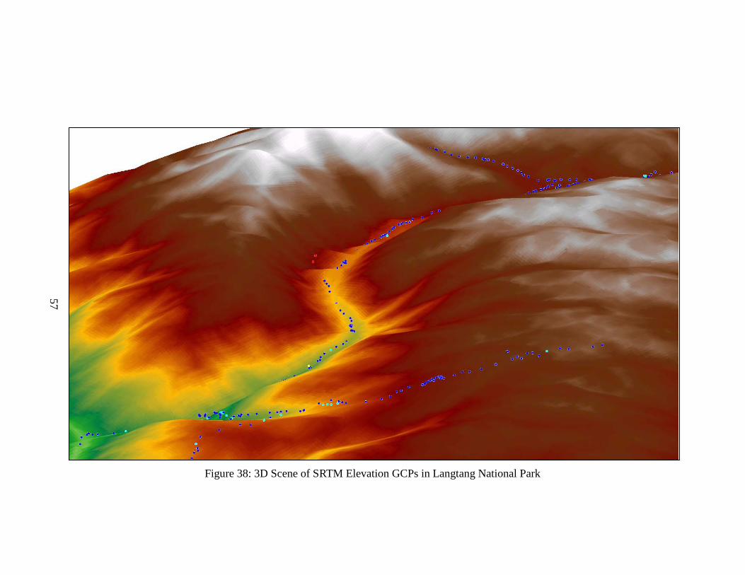
Figure 38. 3D Scene of SRTM Elevation GCPs in Langtang National Park .....................57

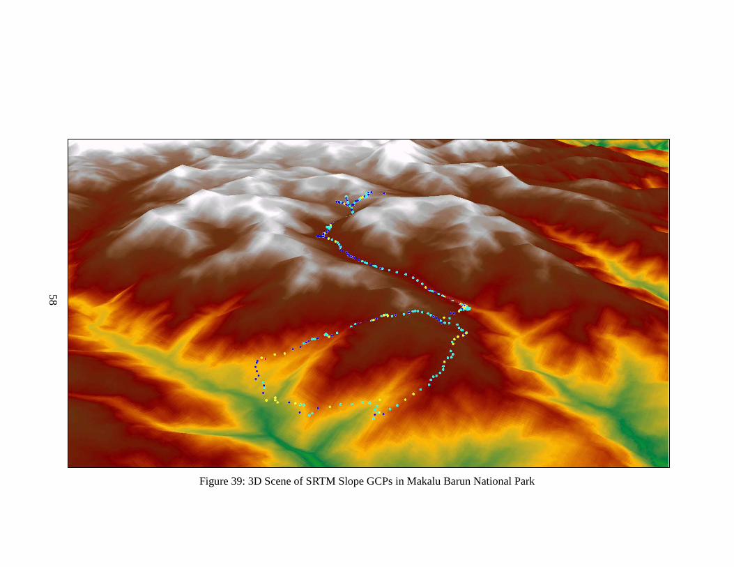
Figure 39. 3D Scene of SRTM Slope GCPs in Makalu Barun National Park ...................58

Figure 40. 3D Scene of SRTM Aspect GCPs in Sagarmatha National Park .....................59

Figure 41. Ridge Top with Low Topographic Variation ....................................................61

Figure 42. Broad Valley with Medium Topographic Variation ..........................................62

Figure 43. Hill Slope with High Topographic Variation ....................................................62

vii

LIST OF TABLES

Table 1. ASTER and SRTM Comparison .......................................................................... 11

Table 2. Nepal Ground Control Points ...............................................................................26 Table 3. SRTM and ASTER Elevation Usable Point Percentages .....................................33 Table 4. SRTM and ASTER Slope Usable Point Percentages ...........................................34 Table 5. SRTM and ASTER Aspect Usable Point Percentages .........................................35 Table 6. SRTM and ASTER Total Usable Points for Elevation, Slope, and Aspect ..........35

viii

GLOBAL DIGITAL ELEVATION MODEL ACCURACY ASSESSMENT IN THE HIMALAYA, NEPAL

Luke Miles December 2013 122 pages Directed by: Dr. John All, Dr. Greg Goodrich, and Dr. Jun Yan Department of Geography and Geology Western Kentucky University

Digital Elevation Models (DEMs) are digital representations of surface

topography or terrain. Collection of DEM data can be done directly through surveying

and taking ground control point (GCP) data in the field or indirectly with remote sensing

using a variety of techniques. The accuracies of DEM data can be problematic, especially

in rugged terrain or when differing data acquisition techniques are combined. For the

present study, ground data were taken in various protected areas in the mountainous

regions of Nepal. Elevation, slope, and aspect were measured at nearly 2000 locations.

These ground data were imported into a Geographic Information System (GIS) and

compared to DEMs created by NASA researchers using two data sources: the Shuttle

Radar Topography Mission (STRM) and Advanced Spaceborne Thermal Emission and

Reflection Radiometer (ASTER). Slope and aspect were generated within a GIS and

compared to the GCP ground reference data to evaluate the accuracy of the satellite-

derived DEMs, and to determine the utility of elevation and derived slope and aspect for

research such as vegetation analysis and erosion management. The SRTM and ASTER

DEMs each have benefits and drawbacks for various uses in environmental research, but

generally the SRTM system was superior. Future research should focus on refining these

methods to increase error discrimination.

1

Chapter 1

Introduction As societies become more concerned about global environmental changes,

environmental analysis is needed to better inform policy responses in both the developed

and developing world. One limitation for environmental studies in developing countries

is the lack of accurate datasets (Goncalves and Fernandes, 2005; Liu, 2008; Ustun et al.,

2006). In recent years, the use of satellite-derived data has become crucial in bridging

the gap for environmental studies across the globe. Topographic datasets, such as Digital

Elevation Models (DEMs), can be generated from orbiting remote sensing platforms

(Tulu, 2005). Quantitative physical properties of geography like elevation, slope, and

aspect can be derived from remote sensing data and are important when studying the land

cover and land use of an area (Saha et al., 2005). For example, many plants and various

crops are limited to certain elevations, and agriculture is difficult to establish in locations

with steeper slopes (Sesnie et al., 2008). Products such as slope and aspect can be

derived from the original DEM. However, these data are highly dependent on landscape

characteristics, because altitude errors in the DEM are exacerbated in the derived

calculations (Aniello, 2003).

The purpose of this study is to compare the elevation, slope, and aspect values

from DEMs created by the Advanced Spaceborne Thermal Emission and Reflection

Radiometer (ASTER) – a passive sensor on the Terra satellite that uses stereoscopic

correlation techniques to create a DEM – and the Shuttle Radar Topography Mission

(SRTM) – a space shuttle mission that utilized radar to create a DEM – to data collected

on the ground in several national parks and conservation areas in Nepal. The primary goal

2

is to determine the usability of remotely sensed measurements of these quantitative

topographical properties (slope and aspect) through error assessment, and to develop an

understanding of the limitations involved. This was done by measuring the magnitude of

the error between the ground data and the remote sensing data, and then distributing the

magnitude of error into classes.

The geospatial data from the study areas were analyzed using Geographic

Information Systems (GIS), remote sensing analysis, and Ground Control Points (GCPs).

A GIS is a computerized system used to collect, correct, store, analyze, and manipulate

geospatial data to create maps, charts, and reports (Chang, 2010). Qualitative remote

sensing analysis was used to analyze the error difference between the remote sensing

platform data and the GCP data in six protected areas of Nepal. The error difference

between the GCPs and the DEMs was used to create a spectrum of confidence for

evaluating the remote sensing data products. The data have been classified as: Definitely

Useable, Provisionally Useable, or Not Useable. By utilizing data gathered in the field

and examining the variability of the landscape, this study provides a basis of

understanding for current and future environmental assessment applications of global

DEM datasets.

Although increased use of remote sensing technology has brought about a better

understanding of the Earth, consistent refinement and improvement of global DEMs are

needed to further research and analysis (Holmes et al., 2000). With space-borne earth-

observation sensors, it is possible to generate DEMs with near-global coverage of the

Earth's surface (Huggel et al., 2007). DEMs are an effective way to examine terrestrial

features and are important for different analytical techniques, including three-dimensional

3

GIS, environmental monitoring, and geo-spatial analysis (Gorokhovich and Voustianiouk,

2006; Nikolakopoulos and Chrysoulakis, 2006). The accuracy of these derived products

depends upon the quality and pixel size of the DEM and is of paramount importance for

environmental issues, especially in areas of rough topography such as mountain ranges.

Due to accuracy issues, slope and aspect data in DEM-based environmental research have

often not been utilized in spite of the significant role of both slope and aspect for

vegetation, hillside stability, etc. (Bennie et al., 2006). Instead, many studies choose to

normalize the land surface variables to remove the slope and aspect components because

of these accuracy concerns (Hale and Rock, 2003).

Slope and aspect are critical components for environmental hazard assessment.

Any significant change in slope and aspect can have a major impact on local environment

risk. For example, slope failure is often tied to the angle of repose (the steepest angle at

which the sloped surface of a given material is stable). Any differences in the structure or

moisture content of the slope material changes the angle of repose. Understanding the

characteristics of the materials, as well as the bio-climate setting (e.g. weather,

vegetation), is paramount in assessing slope processes (Carson, 1969). For example,

depending on the slope materials, a 5° error on a 30° slope is just as dangerous as a 5°

error on a 60° slope. Providing they are both near the failure point, the absolute angle is

not as important as the proximity of the angle to collapse. Thus, classes of error, rather

than actual absolute error values, were used in this analysis.

The presence of soil moisture and vegetation influences the angle of repose as

well. Soil moisture decreases the angle of repose and vegetation increases the angle of

repose. Aspect is critical in this regard because these parameters vary depending on sun

4

angle. In cold, mountainous regions, south-facing slopes will have higher angles of

repose than north-facing slopes because vegetation grows on slopes with direct sunlight

(Figure 1), and because these southern aspects will tend to hold less moisture in these

mesic environments as well.

Figure 1: Influence of elevation, slope and aspect on human settlements in Sagarmatha

National Park (Photo provided by Dr. John All)

5

Chapter 2

Background

To understand environmental change at any significant scale – local, regional or

global – the importance of recognizing the inherent connections to geography cannot be

overstated. Geography provides an appropriate context for environmental inquiries such

as land use / land cover change, climate change, and human / landscape interaction.

Geography embraces the relationships and differences in scale between humans and their

environment. This keeps geography relevant in the development of new environmental

applications through research, application, and public participation (Liverman, 2004).

As technology has developed, geographical methods and techniques have grown

along with it. The development and use of spatial reference systems has strengthened

geography analysis to better showcase changes across the global landscape. These spatial

systems compare the relationships between discrete locations, visualize the dynamics of

these locations (i.e. climate, population), and enhance our understanding of the

relationship between humans and their environment in terms of land use / land cover and

biodiversity. The development of GIS, as both a tool and a science, has directly

contributed to the advancement of geography and is used to quantify these spatial

relationships.

DEMs are used to research and monitor geographic and meteorological

phenomena in more remote and dangerous areas, where direct measurement would be

very difficult. In terms of elevation, slope, and aspect, varied topography can impair

accuracy with respect to glacial monitoring (Kääb et al., 2002), floods (Sanyal and Lu,

2005), landslides (Liu et al., 2004), volcanoes (Huggel et al., 2008), as well as overall

6

hazard assessment (Tralli et al., 2005). Validating the accuracy of DEMs and assessing

error generation is critical for research usage of these datasets. Better technology allows

for greater ease in the generation of DEMs, but offers little help in evaluating the quality

of the output (Cooper, 1998). Due to the increasing use of automation techniques,

effective quality control becomes more difficult because the algorithms used in these

calculations are not able to ‘self-check’ and determine when they are working correctly or

when they fail (Heipke, 1999).

2.1 Remote Sensing and DEMs

Remote sensing is a crucial part of the advancement of geography as a discipline.

Geographers use remote sensing as a tool to better understand distant areas, and to

document environmental changes. It is defined by Schowengerdt (2007, p. 2) as, “...the

measurement of object properties on the earth's surface using data acquired from planes

or satellites”. Remote sensing for image processing and interpretation allows for

environmental analysis without having to physically go to an area. The images used in

remote sensing analysis depend on the size of the study area. Low-flying aircraft can

provide data for smaller areas; but for larger areas, earth-orbiting satellites gather the

remote sensing imagery. Remote sensing is especially useful when dealing with isolated

and often dangerous areas, such as high mountain ranges.

Remote sensing applications can profound impact our understanding of global

environmental change. The imagery can reveal changes across both space and time. For

example, in environmentally sensitive areas such as the mountainous regions of Nepal,

remote sensing can document changes in the landscape due to glacial recession. That, in

7

turn, can influence the development of human settlements, agriculture, grazing areas, and

tourist attractions. Since remote sensing imagery is broken up into spectral bands, it can

also be used for land classification. These bands can be analyzed to show the general type

of plants present, the overall health/vigor of the plants, the amount of soil moisture in the

area, and anthropogenic impacts on various environmental parameters. These datasets can

then be longitudinally studied across time for changes in plant biodiversity as a response

to human impacts, natural disturbances, and climate change.

There are two types of methods through which remote sensing platforms acquire

data: active and passive. The fundamental difference between the two is that while

passive sensors only receive electromagnetic radiation, either reflected off objects from

the sun or emitted from objects on the ground, active sensors emit electromagnetic energy

and use the strength of the return wave to determine physical characteristics of objects, as

well as their distance.

Both active and passive sensors are used to create DEMs (Figure 2). A DEM is a

three-dimensional representation of a terrain's surface, similar to a topographic map. The

quality of the DEM is a measurement of both absolute accuracy – how accurate the

elevation is at each pixel – and relative accuracy – how accurate is the surrounding

morphology. The spatial resolution, or pixel size, of the DEM determines the amount of

data aggregated into each pixel. When the pixels are large, there is significant data

aggregation that smoothes the terrain surface. When the pixels are small, there is less data

aggregation and the terrain surface model has a higher level of detail.

8

Radio Detection and Ranging (RADAR) active systems are useful for measuring

terrain characteristics in areas of frequent cloud cover and thick vegetation. Active

sensors penetrate cloud cover and tree canopies to detect the ground surface (Jensen,

2005). See Figure 2 for an example of the use of a RADAR-based DEM.

Figure 2: The SRTM Digital Elevation Model for the Country of Nepal

The Shuttle Radar Topography Mission (SRTM) occurred during a NASA space

shuttle flight in 2000. The SRTM is an active remote sensing platform which utilizes two

different instruments – one in the shuttle payload bay and one connected to the shuttle via

a 60 meter (m) mast – to measure topographical characteristics. This configuration

creates a radar interferometer - which is similar to stereoscopic correlation. (Farr et al.,

2007) (Figure 3). The mission was to obtain topographic data of the majority of the

9

Earth’s land surfaces (Rabus et al., 2003) and according to NASA, the SRTM collected

data from nearly 80 percent of the Earth (Table 1). The SRTM DEMs are processed at a

pixel size of 30 m in the United States and 90 m for the rest of the world (Corchete et al.,

2006) (Table 1).

Figure 3: SRTM Configuration (Source: SRTM, 2013)

The Advanced Space-borne Thermal Emission and Reflection Radiometer

(ASTER) sensor was originally launched in December 1999 as part of NASA’s Earth

Observing System on the Terra Spacecraft. The ASTER sensor passively measures

fourteen bands from the visible spectrum to the Thermal Infrared. ASTER has three

different ground resolutions: 15 m for visible and Near-Infrared (NIR), 30 m for

Shortwave Infrared (SWIR), and 90 m for Thermal Infrared (TIR) (Bolch et al., 2005;

Jensen, 2005). ASTER creates its DEM by using two camera sensors, one pointed

10

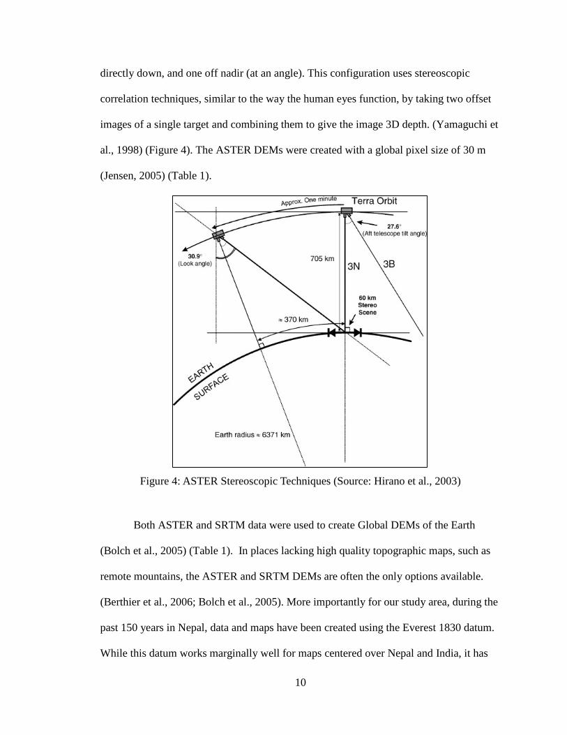
directly down, and one off nadir (at an angle). This configuration uses stereoscopic

correlation techniques, similar to the way the human eyes function, by taking two offset

images of a single target and combining them to give the image 3D depth. (Yamaguchi et

al., 1998) (Figure 4). The ASTER DEMs were created with a global pixel size of 30 m

(Jensen, 2005) (Table 1).

Figure 4: ASTER Stereoscopic Techniques (Source: Hirano et al., 2003)

Both ASTER and SRTM data were used to create Global DEMs of the Earth

(Bolch et al., 2005) (Table 1). In places lacking high quality topographic maps, such as

remote mountains, the ASTER and SRTM DEMs are often the only options available.

(Berthier et al., 2006; Bolch et al., 2005). More importantly for our study area, during the

past 150 years in Nepal, data and maps have been created using the Everest 1830 datum.

While this datum works marginally well for maps centered over Nepal and India, it has

11

significant limitations due to the age of the datum and its incompatibility with modern

Global Navigation Satellite Systems (GNSS) - which use earth-centered datums (e.g.

World Geodetic System 1984 (WGS84)) (Srivastava and Ramalingam 2006). These

Global DEMs use WGS84 and are thus compatible with other geospatial datasets and

represent a significant step forward for environmental analysis.

Table 1: ASTER and SRTM Comparison

Parameters SRTM3 ASTER GDEM Data Source Space Shuttle Radar ASTER

Generation and Distribution NASA/USGS METI/NASA Release Year 2003 2009

Data Acquisition Period 11 days (in 2000) 2000 - Ongoing Posting Interval 90 m 30 m

DEM Accuracy (St. Dev.) 10 m 7-14 m DEM Coverage 60° North - 56° South 83° North - 83° South

Source: METI, 2012

For accuracy assessment of elevation data, comparisons between SRTM, ASTER

and existing topographic maps have been carried out in the past (Van Niel et al., 2008),

but none of these studies have compared these DEMs to actual GCPs as has been done

during this thesis research. Several studies focused on the quantification of non-

conformity between SRTM and other higher resolution DEMs (Hofton et al., 2006;

Rodriguez et al., 2006). Bolch et al., (2005) found better accuracy of ASTER DEMs for

complex land features like high mountain areas, but SRTM DEMs overall has more

precise elevations. It was also noted that a large number of GCPs could increase

accuracy. The study also suggests possible causal factors of errors include steep slopes,

aspect impacts on vegetation, and clouds/cloud shadows. In a comparison between

SRTM and ASTER DEMs, Huggel et al. (2007) found SRTM data to be more reliable in

12

spite of its lower spatial resolution, and identified deeply incised gorges with north-facing

slopes as particularly problematic in ASTER DEM data. Kääb (2005) provided a similar

comparison of the two systems and found the SRTM DEM contains fewer errors than the

ASTER DEM; with error differences in the hundreds of meters. Additionally, Sharma et

al. (2010) suggests the ASTER DEM to be more accurate for highly rugged terrain,

whereas the SRTM DEM is more accurate for predominantly flat landscapes. The study

adds that for high mountain areas, elevation data from both SRTM and ASTER DEMs

are similar to each other, but significantly different from physical topographic maps.

Nikolakopoulos and Chrysoulakis (2006) found that DEMs generated by ASTER and

SRTM are satisfactory and adds that the accuracy of the ASTER DEM is appropriate for

updating 1:50000 topographic maps. Liu (2008) found SRTM DEM data to be of high

quality and concludes that the SRTM DEM can be used to replace 1:250000 topographic

DEMs in most landscapes, including high mountain areas. The study also found that the

SRTM DEM, compared to ground survey data, showed less than 5 m elevation error in

flat areas, and higher errors in mountains. This suggests that slope and aspect are

important factors behind these errors (e.g. northern slopes were more prone to errors than

southern slopes). According to Tulu (2005), the SRTM DEM is more accurate than the

ASTER DEM when compared using the triangulation of GCPs and GPS data; whereas

the ASTER DEM, due to its high resolution, provides much more ground feature details

than SRTM DEM. Tulu (2005) also suggests that depending on the area of interest,

ASTER and SRTM DEMs can vary significantly.

13

There are multiple applications for DEMs; including their use in vegetation

analysis, change detection, and agriculture and land classification. Van Niel et al. (2008)

tested the use of DEMs in predictive vegetation modeling and determined error

propagation of the DEM based on both topographic and environmental factors. They

found that environmental factors, such as slope steepness and cloudiness, can increase

error propagation in subsequent calculations from a base DEM. Eiumnoh and Shrestha

(2000) demonstrate the use of a DEM that compared characteristics of tropical wet-dry

climates in southeast Asia. The DEM greatly assists in land classification during the wet

season, which is typically hampered by frequent cloud cover.

2.2 Study Areas

2.2.1 The Himalaya

The Himalaya are the highest and most massive mountain range in the world.

Over one hundred mountains in this range exceed 7,200 m in height and several exceed

8,000 m in height (Yang and Zheng, 2004). This range includes the tallest mountain in the

world, Mount Everest. The mountain system runs east-to-west and covers a length of

roughly 2,400 kilometers (km), and an area of roughly seven million square kilometers

(sq. km) (Singh et al., 2008; Xu et al., 2009). This range stretches across Nepal, Bhutan,

northern Afghanistan, northern India, northern Pakistan, and the Tibetan Plateau of

China. The Himalaya are home to more than 100 million people; some of who live parts

of the year at altitudes above five thousand meters (Shrestha, 2005). This remote area

attracts people from all over the world who wish to experience the unique mountain

cultures and environment.

14

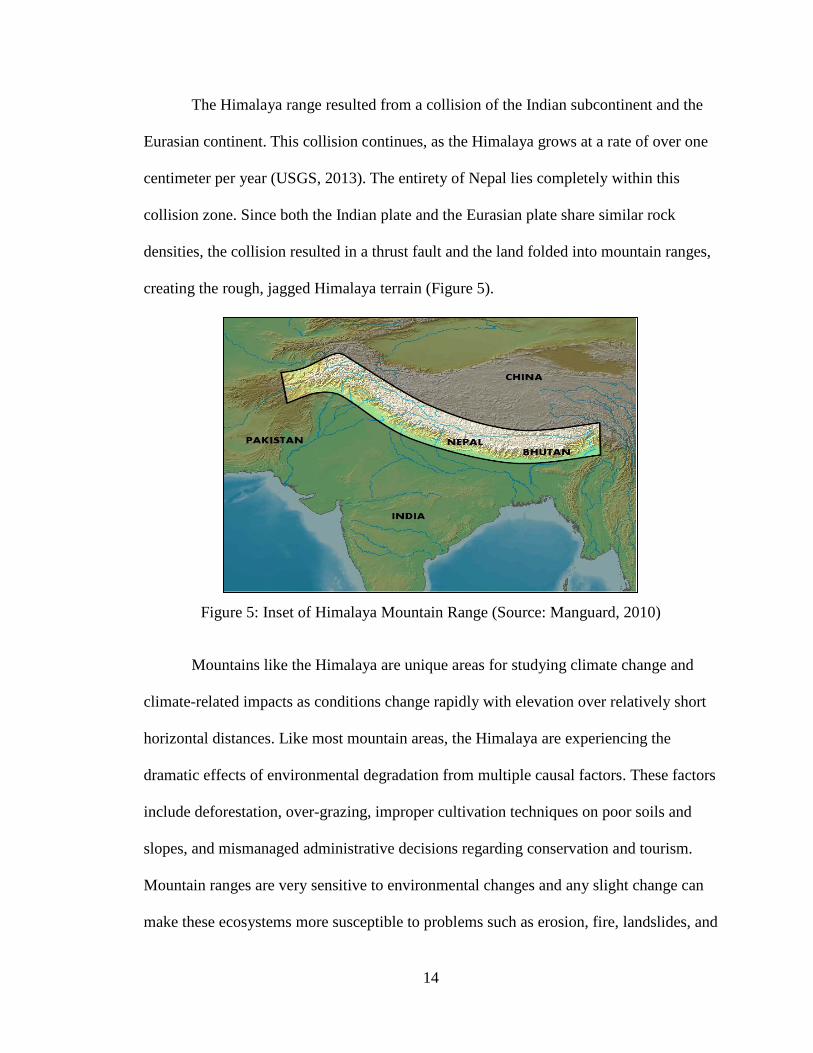
The Himalaya range resulted from a collision of the Indian subcontinent and the

Eurasian continent. This collision continues, as the Himalaya grows at a rate of over one

centimeter per year (USGS, 2013). The entirety of Nepal lies completely within this

collision zone. Since both the Indian plate and the Eurasian plate share similar rock

densities, the collision resulted in a thrust fault and the land folded into mountain ranges,

creating the rough, jagged Himalaya terrain (Figure 5).

Figure 5: Inset of Himalaya Mountain Range (Source: Manguard, 2010)

Mountains like the Himalaya are unique areas for studying climate change and

climate-related impacts as conditions change rapidly with elevation over relatively short

horizontal distances. Like most mountain areas, the Himalaya are experiencing the

dramatic effects of environmental degradation from multiple causal factors. These factors

include deforestation, over-grazing, improper cultivation techniques on poor soils and

slopes, and mismanaged administrative decisions regarding conservation and tourism.

Mountain ranges are very sensitive to environmental changes and any slight change can

make these ecosystems more susceptible to problems such as erosion, fire, landslides, and

15

avalanches. These issues have contributed to an overall loss of habitat and biodiversity in

recent times.

Tourism is a large and lucrative business in the Himalayan range. The

combination of so many of the tallest mountains in the world, as well as the unique

mountain ecosystems in the area, creates attractive recreational opportunities. However,

increased tourist activity, coupled with the effects of climate change, is making these

environmentally fragile areas even more prone to degradation. This problem is worsened

by economic development that is overriding conservation, which leads to further

mountain ecosystem impacts (Baral et al., 2007). Beniston (2003) ties the increased use

of the natural environment to population and economic growth. Both of these factors play

a larger role in environmental degradation in less affluent mountain countries.

Byers (2009) examined the important issue of how the local populations respond

to economic incentives for practicing methods of conservation. The combination of

economic underdevelopment, poverty, land access, and environmental degradation have

made influencing target populations with conservation initiatives and best management

practices very difficult and time intensive. Nepal's national parks and conservation areas

are home to thousands of people who lived and worked there before the land was

designated as a protected area and they do not respond favorably to the changes in their

livelihood. Sustainable alternatives have been proposed, but have been largely considered

unaffordable by local villagers, in spite of their recognition of the importance of

protecting natural resources (Mahal, 1988).

16

2.2.2 Nepal

Nepal (27° 42′ N, 85° 19′ E) is a country located in Southern Asia. It is bordered

by China in the north, and India in the south, east, and west. Nepal lies along the

Himalaya mountain range that runs east to west. The country measures ~800 kilometers

across its east-west axis and only ~200 kilometers across its north-south axis. Nepal

experiences dramatic land use/land cover changes as the terrain rises from a base

elevation near sea level to the peak of Mount Everest. This significant gradient creates

unique diversity in the country’s plants, animals, and ecosystems.

This diversity correlates with variability in hydrology and microclimate.

(Whiteman, 2000). This means that the Himalaya contain incredible biodiversity in small

climate belts (Beniston, 2003). Unfortunately, any change to this delicate ecosystem can

make the region more susceptible to fire, soil erosion, landslides, avalanches, and the loss

of both habitat and biodiversity (Becker et al., 2007; Beniston, 2003; Byers, 2009;

Lambin and Geist, 2006).

Nepal’s land is traditionally split into three sections: the Terai Region, the Hill

Region, and the Mountain Region (Chakraborty, 2001). The Terai Region contains the

lowlands along the southern border with India and ends in the foothills (~600 m)

(Bhattarai and Vetaas, 2003; Mugnier et al., 1999). The Terai has a humid subtropical

climate. Due to its low elevation and gentle slope, this area has dense forests and marshy

grasslands and savannas. The Hill Region lies between the Terai and Mountain regions at

elevations from ~600 m to ~2,500 m (Mugnier et al., 1999). This area begins the

transition between the lowlands and the alpine sections of the country. The Hill Region

has a subtropical highland climate. This region ends abruptly when the Himalaya

17

Mountains quickly begin to rise thousands of meters. The Mountain Region begins at

~2,500 m and rises to over 8,000 m (Gurung and Bajracharya, 2012). The climate in this

region ranges from subarctic/taiga to tundra as seen in Figure 6.

Nepal has a total of ten national parks and six conservation areas. Most of these

parks are UNESCO World Heritage sites, and are managed by the Department of

National Parks and Wildlife Conservation (DNPWC) and the Ministry of Forests in

Nepal. This study examines four national parks and two conservation areas in the hopes

of linking this topographic research to other environmental studies in these protected

areas.

Figure 6: The Köppen-Geiger Climate Classification for the Country of Nepal

18

2.2.3 Annapurna Conservation Area

Established in 1992, the Annapurna Conservation Area (CA) (28° 46′ 48″ N,

83° 58′ 12″ E) is Nepal’s first and largest conservation area (Aryal, 2005; Khadka and

Nepal, 2010). Located in north-central Nepal and bordered by the Tibetan Plateau of

China, it covers an area of 7,629 sq. km (Bhusal, 2009). Annapurna CA has an altitudinal

range of 7,301 m (Bhuju et al., 2007) (Figure 7). This range is characterized by large,

broad river valleys and ridge tops. This area contains several climate zones, with humid

subtropical climates in the southernmost portions of the area changing into taiga and

tundra climates at higher elevations. It is home to over “1,226 species of flowering plants,

102 mammals, 474 birds, 39 reptiles and 22 amphibians” (NTNC, 2013).

19

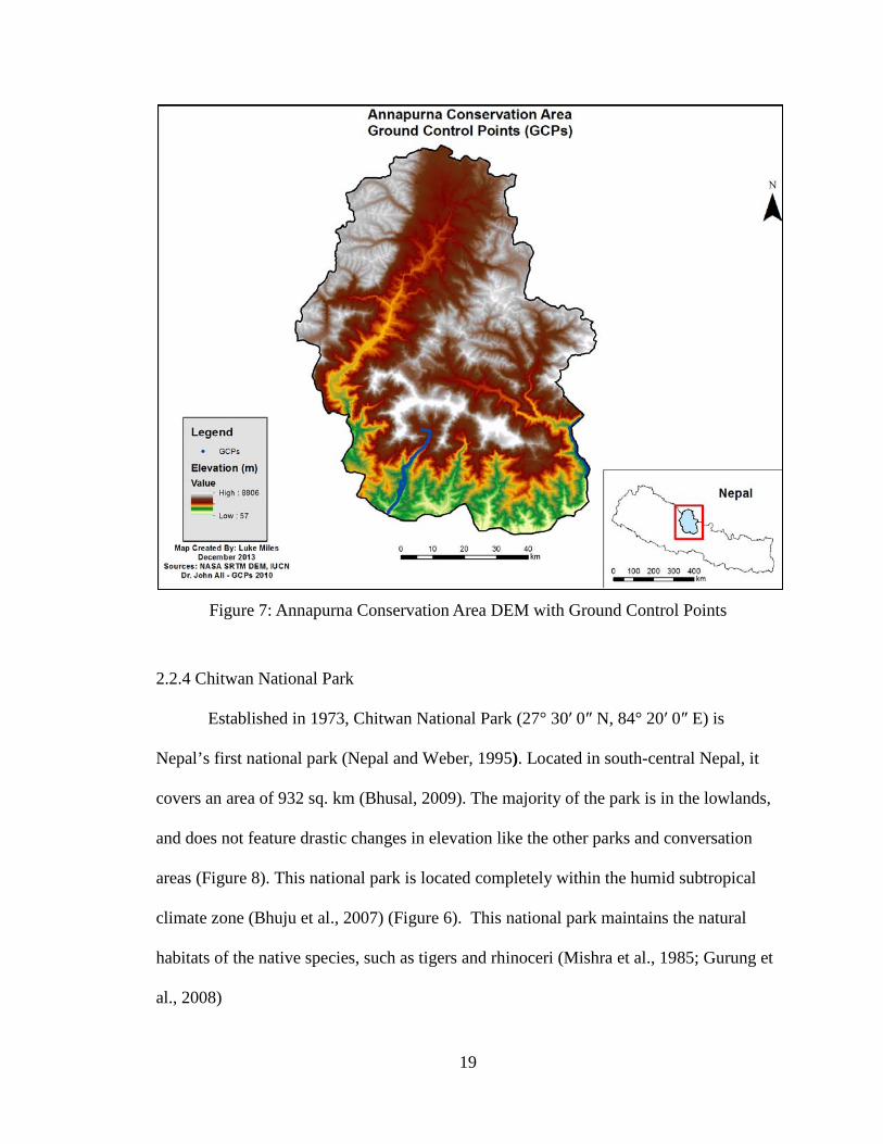
Figure 7: Annapurna Conservation Area DEM with Ground Control Points

2.2.4 Chitwan National Park

Established in 1973, Chitwan National Park (27° 30′ 0″ N, 84° 20′ 0″ E) is

Nepal’s first national park (Nepal and Weber, 1995). Located in south-central Nepal, it

covers an area of 932 sq. km (Bhusal, 2009). The majority of the park is in the lowlands,

and does not feature drastic changes in elevation like the other parks and conversation

areas (Figure 8). This national park is located completely within the humid subtropical

climate zone (Bhuju et al., 2007) (Figure 6). This national park maintains the natural

habitats of the native species, such as tigers and rhinoceri (Mishra et al., 1985; Gurung et

al., 2008)

20

Figure 8: Chitwan National Park DEM with Ground Control Points

2.2.5 Langtang National Park

Established in 1976, Langtang National Park (28° 10′ 25.68″ N, 85° 33′ 11.16″ E)

is Nepal’s first Himalaya national park (Mishra, 2003). The park is located in north-

central Nepal, bordering the Tibetan Plateau of China, and covers an area of 1,710 sq. km

(Bhusal, 2009). The area is comprised of narrow river valleys and steep slopes. It has

climate zone variations similar to Annapurna - with humid subtropical climates in the

southernmost portions of the park progressing to taiga and tundra climates towards the

northern parts of the park. Langtang has an altitudinal range of 6,450 m, which allows

for great variability in biodiversity (Figure 9) (Bhuju et al., 2007).

21

Figure 9: Langtang National Park DEM with Ground Control Points

2.2.6 Sagarmatha National Park

Sagarmatha National Park (27° 56′ 0″ N, 86 ° 44′ 0″ E) was established in 1976

(Byers, 2005). This park is located in northeastern Nepal and it covers an area of 1,148

sq. km (Bhusal, 2009). The altitudinal range of this national park is 6,003 m between the

lowlands and the summit of Mt. Everest (Bhuju et al., 2007). Since the majority of this

park lies above 5,000 m, the climate zones in this area are either taiga or tundra (refer to

Figure 6). The area is very rugged and steep with a few broad valleys (Figure 10).

22

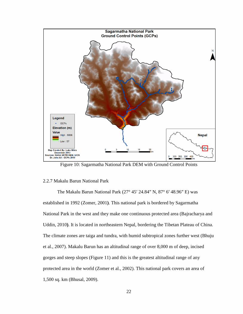
Figure 10: Sagarmatha National Park DEM with Ground Control Points

2.2.7 Makalu Barun National Park

The Makalu Barun National Park (27° 45′ 24.84″ N, 87° 6′ 48.96″ E) was

established in 1992 (Zomer, 2001). This national park is bordered by Sagarmatha

National Park in the west and they make one continuous protected area (Bajracharya and

Uddin, 2010). It is located in northeastern Nepal, bordering the Tibetan Plateau of China.

The climate zones are taiga and tundra, with humid subtropical zones further west (Bhuju

et al., 2007). Makalu Barun has an altitudinal range of over 8,000 m of deep, incised

gorges and steep slopes (Figure 11) and this is the greatest altitudinal range of any

protected area in the world (Zomer et al., 2002). This national park covers an area of

1,500 sq. km (Bhusal, 2009).

23

Figure 11: Makalu Barun National Park DEM with Ground Control Points

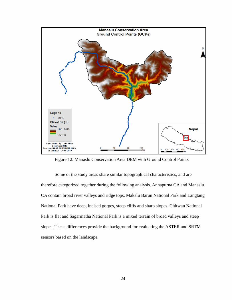
2.2.8 Manaslu Conservation Area

The Manaslu Conservation Area (CA) (28° 32′ 45.6″ N, 84° 50′ 31.2″ E) was

established in 1998 (Bajimaya, 2003). It is located in north-central Nepal, bordering the

Tibetan Plateau of China. It covers an area of 1,633 sq. km (Bhusal, 2009). The park

begins in the lowlands at 600 m and rises to the peak of Mount Manaslu at 8,613 m

(Bhuju et al., 2007) (see Figure 12). This large altitudinal range covers humid continental

as well as taiga and tundra climates. This area contains large river valleys and open

terrain similar to Annapurna CA.

24

Figure 12: Manaslu Conservation Area DEM with Ground Control Points

Some of the study areas share similar topographical characteristics, and are

therefore categorized together during the following analysis. Annapurna CA and Manaslu

CA contain broad river valleys and ridge tops. Makalu Barun National Park and Langtang

National Park have deep, incised gorges, steep cliffs and sharp slopes. Chitwan National

Park is flat and Sagarmatha National Park is a mixed terrain of broad valleys and steep

slopes. These differences provide the background for evaluating the ASTER and SRTM

sensors based on the landscape.

25

Chapter 3

Data and Methodology

3.1 Data

Data for this research was gathered from multiple sources. SRTM DEMs were

obtained from the Consultative Group on International Agriculture Research -

Consortium for Spatial Information (CGIAR-CSI) (http://www.cgiar-csi.org/data/srtm-

90m-digital-elevation-database-v4-1). ASTER DEMs were acquired from the National

Aeronautics and Space Administration (NASA) Global Digital Elevation Model (GDEM)

project (http://asterweb.jpl.nasa.gov/gdem.asp). The International Union for the

Conservation of Nature (IUCN) provided the Nepal GIS shapefiles (http://www.iucn.org).

Ground reference data, or GCPs, were collected by Dr. John All in various

national parks and conservation areas in Nepal, which include: Annapurna CA, Manaslu

CA, Chitwan National Park, Langtang National Park, Sagarmatha National Park, and

Makalu Barun National Park. These study areas were chosen to represent areas that vary

significantly in terms of elevation, slope, and aspect - with data collected in both a

lowland site (Chitwan National Park) and mountainous regions. Data collected in the

lowlands provided a reference point to compare to the analysis in the rugged areas.

A total of over 1,800 GCPs were collected from 2009-2010 across the country of

Nepal. The instruments used to acquire these GCPs were a Garmin60CSx GPS for

elevation, an inclinometer for slope, and a sighting compass for aspect. The derived slope

and aspect data for each point were averaged with a radius of 10 m. The GCPs were

collected using a stratified random protocol using fixed linear distances and elevation

changes from a random starting point. Additionally, opportunistic points were collected

26

whenever a distinct land feature such as ridges, valleys, forests, bare land, grasslands, and

developed settlements were encountered in order to provide a more robust dataset. The

study areas had very few flat locations, and the greater likelihood of error made them

more compelling research areas for evaluating accuracy thresholds. Table 2 shows the

total number of GCPs for the parameters in each park and conservation area respectively.

Table 2: Nepal Ground Control Points

Area of Interest Elevation GCPs Slope GCPs Aspect GCPs Annapurna Conservation Area 165 141 141

Chitwan National Park 145 197 0 Langtang National Park 326 178 77

Makalu Barun National Park 262 262 234 Manaslu Conservation Area 562 357 389 Sagarmatha National Park 417 389 308

Total 1877 1525 1149

3.2 Methods

Further refinement of the dataset was conducted on both the DEMs and GCPs in

ArcGIS™ Desktop. The ASTER and SRTM DEMs were originally obtained as separate

files and were mosaicked together into single images. Once each image was mosaicked,

copies were projected into the Universal Transverse Mercator (UTM) coordinate system

– both Zone 44 North and Zone 45 North due to the fact that these two zones bisect the

country. Subsequently, both mosaicked images were then clipped to the political borders

of Nepal, and the proper zone image was used for each park.

The slope and aspect layers were generated in ArcMap® utilizing the Spatial

Analyst™ extension. The surface analysis tool was used to create both slope and aspect

terrain from the ASTER and SRTM DEMs. The slope terrain was derived by evaluating

the rates of change in the horizontal and vertical directions across a three-by-three cell

27

neighborhood. The aspect terrain was derived by evaluating the rates of change in the x-y

directions across a three-by-three cell neighborhood. Each GCP point layer was projected

into UTM 45N for the majority of the points (in central and eastern Nepal) and UTM 44N

for Annapurna CA. Once they were in the correct projection, the GCPs were overlaid on

top of the elevation, slope, and aspect layers for the ASTER and SRTM DEMs. The

‘Extract Values to Points’ tool in the Spatial Analyst™ extension was then used to extract

the elevation, slope, and aspect data based upon the location of the GCP point features.

This tool added a new field to the attribute table of the GCP point data and then populated

it with the value of the cell being sampled. These values were all imported into Microsoft

Excel for further comparative analysis.

3.2.1 Slope Classification

In determining the usability of the slope data, the magnitude of the error between

the measured GCP data (Actual) and the satellite-derived data (Observed) was calculated.

This created both positive and negative values and so the absolute value of each error was

calculated to leave only the magnitude of the error. Next, these errors were comparatively

scaled against the ground data, which determined their overall usability. Each data point

was scaled and categorized in 5° intervals from 0-90°. The intervals were based on the

standard error of the ASTER and SRTM platform.

Eighteen classes were created using this interval. This technique appropriately

scaled and categorized the magnitude of the error. To be considered useable, the error

value had to be within the standard error of the ASTER or SRTM DEM instrument

parameters and since each class was delineated in the classes of 5° intervals, the

28

magnitude of error had to be within the first two classes, or less than 10°, to be

considered useable. Any point that was above the 10° limit was considered a significant

error in derived slope.

3.2.2 Aspect Classification

Determining the usability of the aspect data was more complicated than the slope

data. The slope data have values from 0-90° with a meaningful, non-arbitrary zero value.

However, aspect data contain values between 0-360° but the 0° value is also equal to

360°. This was an issue when the actual data and the observed data were on opposite

sides of the 0°-line. Two equations were used to effectively split the cyclic data into two

halves. These equations depended on the difference between the actual and observed data

points to negate the effect of the 0°-line in our calculations:

When the actual aspect value was much lower than the observed, this was

indicative of a crossing of the 0°-line from right to left. The actual error difference was

calculated with the following formula.

(360 + Actual) – Observed (1)

When the actual aspect value was much higher than the observed, this was

indicative of a crossing of the 0°-line from left to right. The actual error difference was

calculated with the following formula:

360 – (Actual – Observed) (2)

Figure 13 below demonstrates an example of this issue and how it was solved:

29

Figure 13: Aspect 0°-line Correction Method

Using these two formulas ensured no error values were greater than ±180°. The

absolute value of the difference, similar to slope, was then used. This method reduced the

total number of classes that resulted (36 instead of 72). Each value was then scaled and

categorized in 5° intervals from 0-180°.

Thirty-six classes were thus created for appropriately scaling and categorizing the

magnitude of the aspect errors. To be considered useable, the error value had to be within

the standard error of the ASTER or SRTM DEM instrument parameters. Since each class

was delineated in the classes of 5° intervals, the error had to be within the first two

classes, or less than 10°, to be considered usable. Any errors greater than 10° were

considered a significant change in aspect – and thus solar radiation receipt.

30

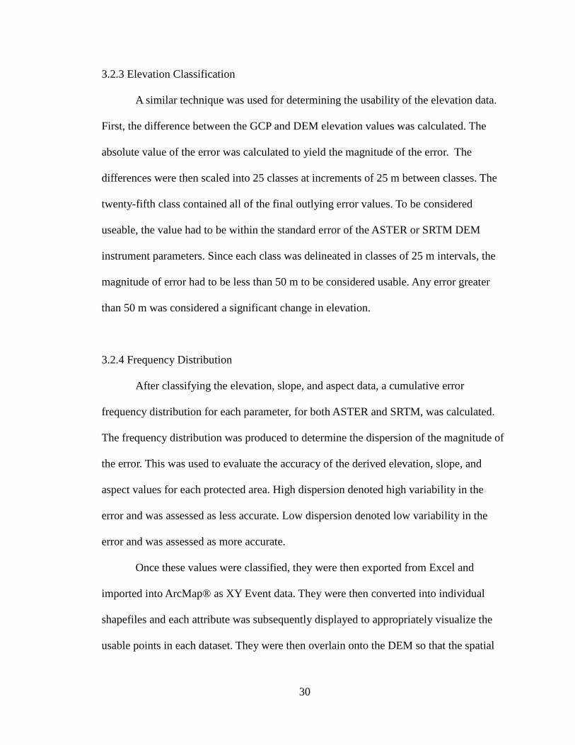
3.2.3 Elevation Classification

A similar technique was used for determining the usability of the elevation data.

First, the difference between the GCP and DEM elevation values was calculated. The

absolute value of the error was calculated to yield the magnitude of the error. The

differences were then scaled into 25 classes at increments of 25 m between classes. The

twenty-fifth class contained all of the final outlying error values. To be considered

useable, the value had to be within the standard error of the ASTER or SRTM DEM

instrument parameters. Since each class was delineated in classes of 25 m intervals, the

magnitude of error had to be less than 50 m to be considered usable. Any error greater

than 50 m was considered a significant change in elevation.

3.2.4 Frequency Distribution

After classifying the elevation, slope, and aspect data, a cumulative error

frequency distribution for each parameter, for both ASTER and SRTM, was calculated.

The frequency distribution was produced to determine the dispersion of the magnitude of

the error. This was used to evaluate the accuracy of the derived elevation, slope, and

aspect values for each protected area. High dispersion denoted high variability in the

error and was assessed as less accurate. Low dispersion denoted low variability in the

error and was assessed as more accurate.

Once these values were classified, they were then exported from Excel and

imported into ArcMap® as XY Event data. They were then converted into individual

shapefiles and each attribute was subsequently displayed to appropriately visualize the

usable points in each dataset. They were then overlain onto the DEM so that the spatial

31

dynamics were revealed across each park. This allowed an examination of the patterns of

usability, with respect to the landscape-type being observed. These shapefiles were also

displayed in ArcScene® to better visualize the elevation, slope, and aspect differences in

3D.

32

Chapter 4

Results and Discussion

4.1 Overall Usability

Tables 3 through 6 show the total numbers and percentages of useable points

found in each protected area for both the ASTER and SRTM datasets. For elevations, the

remote sensing platforms performed well: both SRTM and ASTER in the majority of the

parks had at least 75% usable points. These values were relatively consistent despite the

different landscapes in each park and conservation area. However, since the scaling for

elevation was different from that of slope and aspect, it did not provide a complete

representation of the data. In evaluating slope and aspect from both SRTM and ASTER,

it was obvious that the remote sensing platforms had some difficulty in generating usable

values.

Table 3 shows the elevation usability for the SRTM and ASTER. Each protected

area’s data was evaluated by examining both the total number of useable points and the

percentage of useable points. The useable points for all six protected areas were then

averaged to determine the mean usability for each remote sensing product. The SRTM

performed very well with regards to elevation, with all but Makalu Barun National Park

above 75% usability.

33

Table 3: SRTM and ASTER Elevation Useable Point Percentages

SRTM Elevation Useable Percentage Useable Annapurna Conservation Area 124 75.15% Manaslu Conservation Area 450 80.07%

Langtang National Park 294 90.18% Makalu Barun National Park 87 33.21%

Chitwan National Park 144 99.31% Sagarmatha National Park 368 88.25%

Average 244.50 78.16%

ASTER Elevation Useable Percentage Useable Annapurna Conservation Area 123 74.55% Manaslu Conservation Area 440 78.29%



Average 241.17 77.09%

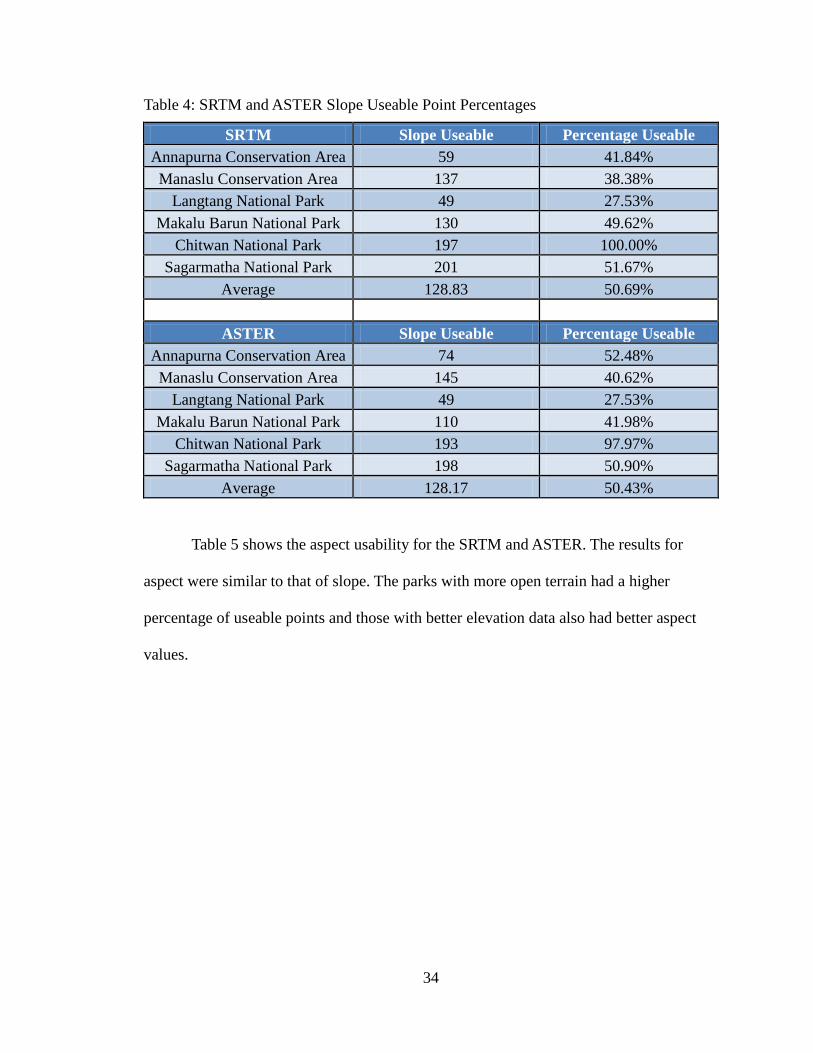
Table 4 shows the slope usability for the SRTM and ASTER. The number of

usable points dropped significantly due to the rugged terrain, and the difficulty of ground

measurements of slope in dangerous terrain. The parks where the satellites performed the

best, excluding Chitwan - which is predominately flat and had the best accuracy values,

were parks with broad river valleys and ridge tops with a large percentage of open sky,

such as Annapurna and Sagarmatha. It was also evident that parks with better elevation

accuracy typically had higher slope accuracy - the more accurate the original DEM, the

more accurate the derived surfaces.

34

Table 4: SRTM and ASTER Slope Useable Point Percentages

SRTM Slope Useable Percentage Useable Annapurna Conservation Area 59 41.84% Manaslu Conservation Area 137 38.38%



Average 128.83 50.69%

ASTER Slope Useable Percentage Useable Annapurna Conservation Area 74 52.48% Manaslu Conservation Area 145 40.62%



Average 128.17 50.43%

Table 5 shows the aspect usability for the SRTM and ASTER. The results for

aspect were similar to that of slope. The parks with more open terrain had a higher

percentage of useable points and those with better elevation data also had better aspect

values.

35

Table 5: SRTM and ASTER Aspect Useable Point Percentages

SRTM Aspect Useable Percentage Useable Annapurna Conservation Area 37 26.24% Manaslu Conservation Area 82 21.08%



Average 37.33 19.50%

ASTER Aspect Useable Percentage Useable Annapurna Conservation Area 30 21.28% Manaslu Conservation Area 70 17.99%



Average 31.17 16.28%

Table 6 shows the comparative total useable points of each remote sensing

product for both the ASTER and SRTM DEM. Looking at the points on a holistic level,

the SRTM performed slightly better than the ASTER data.

Table 6: SRTM and ASTER Total Usable Points for Elevation, Slope and Aspect

Useable Totals Elevation Percentage Useable SRTM 1467 78.16% ASTER 1447 77.09%

Useable Totals Slope Percentage Useable SRTM 773 50.69% ASTER 769 50.43%

Useable Totals Aspect Percentage Useable SRTM 224 19.50% ASTER 187 16.28%

36

4.2 Individual Park Analyses

Figures 14-30 below show the SRTM cumulative error frequency distributions of

all the points in each park for elevation, slope, and aspect through the tenth class. The

tenth class was used as the upper bound for visualization purposes because the majority

of the variance in each park was within the first ten classes. Each GCP error class was

then converted into a percentage of the total points, labeled above each bar, and added

cumulatively. The dispersion of the magnitude of the error was used to evaluate accuracy

for each protected area. When dispersion was low, then the accuracy was assessed as

higher. When dispersion was high, then the accuracy was assessed as lower. The local

topography in each protected area played an important role in terms of error propagation.

Aside from Chitwan, which was predominantly flat and far outperformed all of the other

parks, the mountain areas had difficulties overcoming accuracy issues with regards to

slope and aspect. Because the SRTM performed better than ASTER, only SRTM

distribution results will be discussed here. The general performance patterns between the

two platforms were identical and it would be redundant to discuss both of them. Please

refer to Appendix A for the ASTER ten-class frequency distributions. For the elevation,

slope, and aspect full class cumulative frequency distribution graphs for ASTER and

SRTM, refer to Appendices B and C respectively.

37

Figure 14: Annapurna SRTM Elevation Cumulative Error Frequency Distribution

Figure 15: Annapurna SRTM Slope Cumulative Error Frequency Distribution

75.15

83.03

87.27 90.30 93.94 96.36 98.18 98.79 99.39 100

0.00

20.00

40.00

60.00

80.00

100.00

1 2 3 4 5 6 7 8 9 10

Number of Points

GCP Error Classes

Annapurna SRTM Elevation Cumulative Error Frequency Distribution

16.31 31.21

41.84

55.32 68.79 82.27

88.65 92.91

95.74 97.87

0.00

5.00

10.00

15.00

20.00

25.00

1 2 3 4 5 6 7 8 9 10

Number of Points

GCP Classes

Annapurna SRTM Slope Cumulative Error Frequency Distribution

38

Figure 16: Annapurna SRTM Aspect Cumulative Error Frequency Distribution

Annapurna DEM data performed very well with respect to elevation. Slope and

aspect was not as accurate, but the dispersion of the values was low - which indicated

higher accuracy. Over 80% of Annapurna's elevation values were within the first two

classes (within 50 m of the actual value). Annapurna's topography of broad ridge tops

provided optimal data collection locations.

Figure 17: Chitwan SRTM Elevation Cumulative Error Frequency Distribution

16.31 31.21

41.84

55.32 68.79 82.27

88.65 92.91

95.74 97.87

0.00

5.00

10.00

15.00

20.00

25.00

1 2 3 4 5 6 7 8 9 10

Number of Points

GCP Error Classes

Annapurna SRTM Aspect Cumulative Error Frequency Distribution

49.66 99.31

100 100 100 100 100 100 100 100 0.00

10.00 20.00 30.00 40.00 50.00 60.00 70.00 80.00

1 2 3 4 5 6 7 8 9 10

Number of Points

GCP Error Classes

Chitwan SRTM Elevation Cumulative Error Frequency Distribution

39

Figure 18: Chitwan SRTM Slope Cumulative Error Frequency Distribution

Chitwan's DEM data accuracy levels were clearly the best out of all the parks.

One hundred percent of both elevation and slope data points for this park were within the

first two classes. This was due to the lack of any significant change in topography as

Chitwan is mostly flat. There was no aspect data for Chitwan due to the lack of

significant slopes. Chitwan was chosen to show what was possible when DEMs are

created using remote sensing. This analysis showed how valuable these data are for the

majority of the Earth that has less rugged topography.

Figure 19: Langtang SRTM Elevation Cumulative Error Frequency Distribution

97.46

100 100 100 100 100 100 100 100 100 0.00

50.00

100.00

150.00

200.00

250.00

1 2 3 4 5 6 7 8 9 10

Number of Points

GCP Error Classes

Chitwan SRTM Slope Cumulative Error Frequency Distribution

60.74

90.18

95.40 98.16 98.77 99.08 99.08 99.08 99.08 99.39 0.00

50.00

100.00

150.00

200.00

250.00

1 2 3 4 5 6 7 8 9 10

Number of Points

GCP Error Classes

Langtang SRTM Elevation Cumulative Error Frequency Distribution

40

Figure 20: Langtang SRTM Slope Cumulative Error Frequency Distribution

Figure 21: Langtang SRTM Aspect Cumulative Error Frequency Distribution

Langtang DEM data performed well in terms of elevation, but struggled with

slope and aspect. Over 90% of the total points for elevation were contained within the

first two classes. Although slope and aspect contained over 75% of the points in the first

ten classes, the dispersion of the points was very high, which means that the magnitude of

errors were consistently greater. The higher errors were due to Langtang's deep, incised

river gorges and steep slopes where the majority of the points were collected.

14.04

21.91

27.53 34.83

39.33

47.19 56.74 66.29 76.40

84.83

0.00

5.00

10.00

15.00

20.00

25.00

30.00

1 2 3 4 5 6 7 8 9 10

Number of Points

GCP Error Classes

Langtang SRTM Slope Cumulative Error Frequency Distribution

12.99 24.68

40.26

48.05

51.95

58.44 63.64

70.13 76.62

77.92

0.00 2.00 4.00 6.00 8.00

10.00 12.00 14.00

1 2 3 4 5 6 7 8 9 10

Number of Points

GCP Error Classes

Langtang SRTM Aspect Cumulative Error Frequency Distribution

41

Figure 22: Makalu Barun SRTM Elevation Cumulative Error Frequency Distribution

Figure 23: Makalu Barun SRTM Slope Cumulative Error Frequency Distribution

19.85

33.21 48.09

57.25 64.89

70.99 77.86 84.73

88.17 90.46

0.00 10.00 20.00 30.00 40.00 50.00 60.00

1 2 3 4 5 6 7 8 9 10

Number of Points

GCP Error Classes

Makalu Barun SRTM Elevation Cumulative Error Frequency Distribution

16.79 36.64

49.62

58.02 69.47 79.77

83.97 89.69 94.27

96.56

0.00 10.00 20.00 30.00 40.00 50.00 60.00

1 2 3 4 5 6 7 8 9 10

Number of Points

GCP Error Classes

Makalu Barun SRTM Slope Cumulative Error Frequency Distribution

42

Figure 24: Makalu Barun SRTM Aspect Cumulative Error Frequency Distribution

Makalu DEM data performed the worst out of all the parks. The topography in

Makalu where the data were collected was not conducive to having accurate data. The

majority of the data were collected on steep hill slopes with high mountains on both

sides, which also limited differential correction of the GPS. There was a high amount of

dispersion for the GCP values, which showed the real limitations of these platforms when

collecting these data.

Figure 25: Manaslu SRTM Elevation Cumulative Error Frequency Distribution

4.27

11.97

16.24

22.22

30.34

35.47

42.74

46.15

52.56

60.26

0.00

5.00

10.00

15.00

20.00

1 2 3 4 5 6 7 8 9 10

Number of Points

GCP Error Classes

Makalu Barun SRTM Aspect Cumulative Error Frequency Distribution

54.09

80.07

92.70

95.55 97.33 98.04 98.40 98.93 99.11 99.47 0.00

50.00 100.00 150.00 200.00 250.00 300.00 350.00

1 2 3 4 5 6 7 8 9 10

Number of Points

GCP Error Classes

Manaslu SRTM Elevation Cumulative Error Frequency Distribution

43

Figure 26: Manaslu SRTM Slope Cumulative Error Frequency Distribution

Figure 27: Manaslu SRTM Aspect Cumulative Error Frequency Distribution

Manaslu DEM data performed well; with over 80% of the elevation values within

the first two classes. Manaslu had similar topographic characteristics to Annapurna – i.e.

the topography was less rugged and in a very broad river valley (Figure 12). Most of the

points were within the first ten classes for slope and aspect, which indicated low

dispersion and higher accuracy.

13.45 26.33 38.38

52.66

63.59

71.71 78.43

81.23

87.68

91.32

0.00

10.00

20.00

30.00

40.00

50.00

60.00

1 2 3 4 5 6 7 8 9 10

Number of Points

GCP Error Classes

Manaslu SRTM Slope Cumulative Error Frequency Distribution

11.57

21.08

32.65 43.19

49.61 57.58

64.52

67.61 72.24 76.61

0.00

10.00

20.00

30.00

40.00

50.00

1 2 3 4 5 6 7 8 9 10

Number of Points

GCP Error Classes

Manaslu SRTM Aspect Cumulative Error Frequency Distribution

44

Figure 28: Sagarmatha SRTM Elevation Cumulative Error Frequency Distribution

Figure 29: Sagarmatha SRTM Slope Cumulative Error Frequency Distribution

64.03

88.25

94.96 98.32 99.52 100 100 100 100 100 0.00

50.00 100.00 150.00 200.00 250.00 300.00

1 2 3 4 5 6 7 8 9 10

Number of Points

GCP Error Classes

Sagarmatha SRTM Elevation Cumulative Error Frequency Distribution

22.82

40.00

51.54

59.23 64.62

72.05 78.46 84.87 88.21

93.33

0.00

20.00

40.00

60.00

80.00

100.00

1 2 3 4 5 6 7 8 9 10

Number of Points

GCP Error Classes

Sagarmatha SRTM Slope Cumulative Error Frequency Distribution

45

Figure 30: Sagarmatha SRTM Aspect Cumulative Error Frequency Distribution

In Sagarmatha, over 90% of the elevation points were within the first two classes.

The majority of the slope and aspect values were within the first ten classes, but there

was a generally large dispersion of values. This was due to the mixed landscape in

Sagarmatha that provided a mixture of optimal data collection locations.

4.2.1 Spatial Analysis

Protected areas such as Annapurna, Manaslu and Sagarmatha all share similar

topographical features, but Sagarmatha was more variable with some very deep valleys in

the park. The dispersion in each of these areas was lower, which indicated higher levels

of accuracy in the derived data. The other areas, (e.g. Langtang and Makalu Barun) have

much more jagged and irregular terrain. These parks have steeper slopes and incised

valleys. The dispersion in each of these areas was high, which indicated a lower level of

accuracy in the derived data.

10.39

18.83 28.57 38.64

46.75

51.62 57.79

63.31

72.08 79.55

0.00 5.00

10.00 15.00 20.00 25.00 30.00 35.00

1 2 3 4 5 6 7 8 9 10

Number of Points

GCP Error Classes

Sagarmatha SRTM Aspect Cumulative Error Frequency Distribution

46

Figures 31-36 display a comparative spatial analysis of elevation, slope, and

aspect for the SRTM and ASTER DEM GCPs in each park. These comparisons provide a

spatial representation to further examine why a park’s DEM data performed well or

poorly. Each GCP class was split into four distinct groups. The first class contained the

best two point classes and was designated as definitely useable for most environmental

applications. The other three groups were divided equally - depending on the total

number of classes - for elevation, slope, and aspect and were designated as provisionally

useable (second class group) and not useable (third and fourth class group). Refer to

Appendices D and E for all comparative spatial analysis maps for SRTM and ASTER,

respectively.

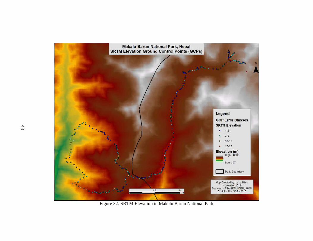
Figures 31 and 32 show the comparison of useable SRTM elevation GCP points in

Langtang National Park and Makalu Barun National Park. This comparison was done

between the park that had the most usable points, and the park that had the least (refer to

Table 3). The points were collected in the western corner of Langtang National Park. The

data collection locations pass through a very broad river valley and then ascend to a ridge

top. Makalu Barun data, on the other hand, began in a shallower valley and elevation

sharply increases. The data collection locations pass through a much shallower valley,

with two high mountain ranges on both sides and the majority of the data points collected

on the slopes of these mountains.

47

Figure 31: SRTM Elevation in Langtang National Park

48

Figure 32: SRTM Elevation in Makalu Barun National Park

49

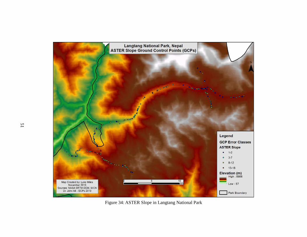
Figures 33 and 34 show the comparison of usable ASTER slope points in

Sagarmatha National Park and Langtang National Park. This comparison was done

between the park that had the most usable points, and the park that had the least (refer to

Table 4). The landscape and data collection locations helped identify the issues between

these two maps. Sagarmatha is an area of mixed terrain with deep river valleys and broad

ridge tops. The mountains were also more north-south oriented in Sagarmatha, and east-

west oriented in Langtang. Many of the points closer to the northwest side of slopes in

Langtang had large errors. Since the ASTER was a passive sensor, any type of shadowing

from north slopes would impair overall accuracy (Berthier et al., 2005).

50

Figure 33: ASTER Slope in Sagarmatha National Park

51

Figure 34: ASTER Slope in Langtang National Park

52

Figures 35 and 36 show the comparison of usable ASTER aspect points in

Annapurna CA and Makalu Barun National Park. This comparison was made between the

park that had the most usable points, and the park that had the least (refer to Table 5). The

landscape in Annapurna was much more open with broad ridge tops. Makalu Barun's

terrain (refer to Figure 11), was much more rugged, with data being collected on the

slopes. Makalu Barun DEM data had a low agreement with elevation data and

consequently had low agreement with the slope and aspect data as well.

53

Figure 35: ASTER Aspect in Annapurna CA

54

Figure 36: ASTER Aspect in Makalu Barun National Park

55

4.2.2 - 3D Visualization

The maps in Figures 37-40 were created in ArcScene® to provide a three-

dimensional representation of elevation, slope and aspect data across the DEM. These

maps were created to improve visualization and analysis. Each map demonstrated the

effect of the topography on the reliability of the terrain. Figures 30 and 31 show that

areas with steeper slopes had less reliable values, while Figures 32 and 33 show that areas

with gentler slopes had more reliable values.

56

Figure 37: 3D Scene of SRTM Elevation GCPs in Annapurna Conservation Area

57

Figure 38: 3D Scene of SRTM Elevation GCPs in Langtang National Park

58

Figure 39: 3D Scene of SRTM Slope GCPs in Makalu Barun National Park

59

Figure 40: 3D Scene of SRTM Aspect GCPs in Sagarmatha National Park

60

Chapter 5

Conclusions and Future Research The availability of a large number of GCPs for this study allowed for a very

detailed accuracy assessment of global DEMs. Considering that Nepal’s topography

varies greatly, the ability to have ground data to verify remotely sensed DEMs is a truly

significant and invaluable opportunity. In Nepal, where people live and work in high

elevations, it is very important to assess the accuracy of these parameters for

environmental management applications. These results can be effectively used to

determine appropriate land use/land cover management strategies for the area in terms of

agriculture, maintaining biodiversity, and hazard assessment.

The local topography of each protected area was crucial to understanding how and

why some park’s data were more accurate than others. Since this was a representative

dataset, with data collected in both the lowlands and in more rugged terrain, evaluating

each park based on the topography was the most effective way to assess the accuracy of

the DEM and the derived slope and aspect terrain data.

Data from topography with low variation, such as the top of a ridge where there

was plenty of open sky, and little to no canopy cover performed the best (Figure 41).

These areas are relatively flat compared to the surrounding landscape, so the magnitude

of the errors for elevation, slope, and aspect should be lower. This is where these DEMs

are most valuable for environmental research.

The valleys between the slopes are secondary in terms of usability – but this

accuracy was entirely dependent on the broadness of the valley and the steepness of the

adjacent slopes. Annapurna, Manaslu, and Sagarmatha had broad river valleys with

61

plenty of open sky, and the magnitude of the errors was lower (Figure 42). The tertiary

locations for data acquisition should be on the steep hill slopes. Depending on the height

and steepness of the slope, these data were generally unusable for most applications

(Figure 43).

Figure 41: Ridge Top with Low Topographic Variation (Photo provided by Dr. John All)

62

Figure 42: Broad Valley with Medium Topographic Variation (Photo provided by Dr.

John All)

Figure 43: Steep Hill Slope with High Topographic Variation (Photo provided by Dr.

John All)

63

The results demonstrated the limitations of DEMs generated from remote sensing

platforms in rugged mountainous areas. The size and coarseness of the pixel was one

possible reason for the error generation. Since the SRTM and ASTER used 90 and 30 m

pixels respectively on a non-uniform and drastically changing landscape, the accuracy of

the terrain data was highly varied depending on its ruggedness. The coarser the spatial

resolution (larger pixels), the smoother the terrain surface, but details of the landscape are

lost. The SRTM has much greater data aggregation of the terrain than the ASTER, but

surprisingly it did not impact the accuracy substantially. Even though data have been

available from each for several years, the research groups that created the datasets still

classify them as research-grade and ongoing improvements are constantly being made.

The metadata clearly informs users of these limitations.

There are potential error issues involved with the ground data as well. Depending

on the location and positional accuracy of the GPS, the error could be somewhat high due

to a lack of satellite reception. This is likely the reason that Makalu Barun National Park

had a considerably lower number of useable points. Considering the topography of

Makalu Barun, which had steep cliffs and incised gorges, the range of the standard error

in the ground data collection was much higher than the other parks. Typically, the other

parks had a GPS standard error that ranged between 4-5 m. Makalu Barun's points had a

GPS error range between 9-10 m. Note: for the entire project, any point location with a

standard error greater than 10 m was discarded. The risk of inaccurate reference data was

greater depending on the range of the error.

64

Another pertinent issue is that the GPS used a barometric altimeter to correct for

elevation. This correction method generally is extremely accurate. However, a rapid

change in barometric pressure can cause fluctuations in the elevation data. The Himalaya

Mountains are subject to strong storms that form quickly and can last for days and data

collection was completed during single expeditions. In an ideal situation, any points that

were collected during a period of rough weather would be retaken during calm weather

and this ‘fair weather’ value would be used.

Evaluating slope and aspect on the ground is also problematic. The topography of

these areas is very rugged and many areas were not easily accessible. At lower elevations,

slope and aspect had to be evaluated through thick jungle vegetation. The landscape is

home to many dangerous plants and animals that endanger the researchers and limit their

movement. At the higher elevations, the steeper, unstable slopes presented a significant

amount of danger of falls and slope collapse.

Another potential factor for error generation was the algorithm that created the

slope and aspect surfaces. Each set of slope and aspect terrain was generated using the

ArcMap® Spatial Analyst™ extension. However, if the original SRTM and ASTER DEM

had erroneous values, then any subsequent calculation magnified the error and skewed

the results. An alternative would be to use additional derivation algorithms to create a

slope and aspect surfaces – e.g. IDRISI or ENVI – and compare the generated surfaces.

The use of ASTER and SRTM DEM had both strengths and weaknesses but the

use of GCPs provided a spectrum of confidence to evaluate the remote sensing DEMs in

terms of overall usability. The use of these platforms in high mountainous areas was a

significant test to assess how both systems performed in particularly difficult

65

environments. The SRTM was more reliable than the ASTER in the protected areas with

broader, more open terrain. The ASTER was more reliable in areas with deep, incised

cliffs and steeper slopes. Understanding the limitations involved in these parameters is

ultimately crucial for quality control in any type of dataset. This study serves as a link to

topographical studies in these areas and DEM use in environmental assessment

applications.

There are several possible future uses for these data. One of these possibilities is

utilizing the DEM to help plot human induced disturbance at each GCP. This can be done

with the use of various clustering methods, such as agglomerative clustering, k-means

clustering, and principle component analysis. Elevation and slope would provide the

foundation for analyzing human-environment interactions in the region.

Another opportunity is a retrospective study using newer DEMs. Currently, the

SRTM-90 m and the ASTER-30 m are the only global DEMs. However, there is a new

project that has been underway for many years that will dramatically improve data

resolution. The European Aeronautic Defense and Space Company (EADS) subsidiary,

Astrium, and the German Aerospace Center (DLR) launched two active remote sensing

platforms in a similar configuration to the SRTM (i.e. an interferometer) to generate a

new global DEM and this data will provide greater accuracy and environmental usability

in the future.

66

APPENDIX A: ASTER 10-Class Cumulative Error Frequency Distribution Graphs

Figure A1: Annapurna ASTER Elevation Cumulative Error Frequency Distribution

Figure A2: Annapurna ASTER Slope Cumulative Error Frequency Distribution

74.55

84.85

88.48 90.91 92.73 94.55 95.76 96.36 96.97 97.58

0.00

20.00

40.00

60.00

80.00

100.00

1 2 3 4 5 6 7 8 9 10

Number of Points

GCP Error Classes

Annapurna ASTER Elevation Cumulative Error Frequency Distribution

15.60

38.30

52.48

62.41 74.47

82.27 87.94 92.91

95.04 96.45

0.00 5.00

10.00 15.00 20.00 25.00 30.00 35.00

1 2 3 4 5 6 7 8 9 10

Number of Points

GCP Error Classes

Annapurna ASTER Slope Cumulative Frequency Error Distribution

67

Figure A3: Annapurna ASTER Aspect Cumulative Error Frequency Distribution

Figure A4: Chitwan ASTER Elevation Cumulative Error Frequency Distribution

Figure A5: Chitwan ASTER Slope Cumulative Error Frequency Distribution

15.60

38.30

52.48

62.41 74.47

82.27 87.94 92.91

95.04 96.45

0.00 5.00

10.00 15.00 20.00 25.00 30.00 35.00

1 2 3 4 5 6 7 8 9 10

Number of Points

GCP Error Classes

Annapurna ASTER Aspect Cumulative Error Frequency Distribution

98.62

99.31 100 100 100 100 100 100 100 100 0.00

20.00 40.00 60.00 80.00

100.00 120.00 140.00 160.00

1 2 3 4 5 6 7 8 9 10

Number of Points

GCP Error Classes

Chitwan ASTER Elevation Cumulative Error Frequency Distribution

77.16

94.92

97.97 97.97 98.98 99.49 100 100 100 100 0.00

20.00 40.00 60.00 80.00

100.00 120.00 140.00 160.00

1 2 3 4 5 6 7 8 9 10

Number of Points

GCP Error Classes

Chitwan ASTER Slope Cumulative Error Frequency Distribution

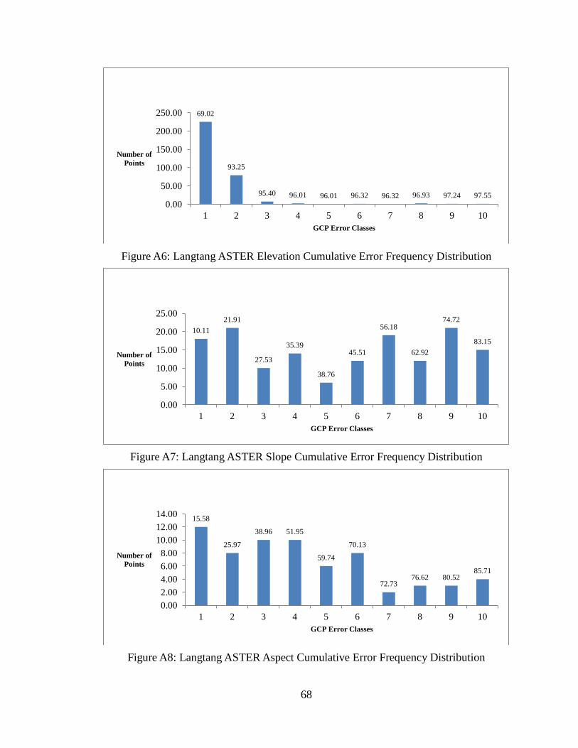
68

Figure A6: Langtang ASTER Elevation Cumulative Error Frequency Distribution

Figure A7: Langtang ASTER Slope Cumulative Error Frequency Distribution

Figure A8: Langtang ASTER Aspect Cumulative Error Frequency Distribution

69.02

93.25

95.40 96.01 96.01 96.32 96.32 96.93 97.24 97.55 0.00

50.00

100.00

150.00

200.00

250.00

1 2 3 4 5 6 7 8 9 10

Number of Points

GCP Error Classes

Langtang ASTER Elevation Cumulative Error Frequency Distribution

10.11 21.91

27.53

35.39

38.76

45.51

56.18

62.92

74.72

83.15

0.00

5.00

10.00

15.00

20.00

25.00

1 2 3 4 5 6 7 8 9 10

Number of Points

GCP Error Classes

Langtang ASTER Slope Cumulative Error Frequency Distribution

15.58

25.97

38.96 51.95

59.74

70.13

72.73 76.62 80.52

85.71

0.00 2.00 4.00 6.00 8.00

10.00 12.00 14.00

1 2 3 4 5 6 7 8 9 10

Number of Points

GCP Error Classes

Langtang ASTER Aspect Cumulative Error Frequency Distribution

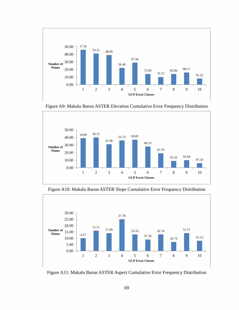
69

Figure A9: Makalu Barun ASTER Elevation Cumulative Error Frequency Distribution

Figure A10: Makalu Barun ASTER Slope Cumulative Error Frequency Distribution

Figure A11: Makalu Barun ASTER Aspect Cumulative Error Frequency Distribution

17.56 33.21 48.09

56.49

67.56

72.90 76.72

82.06 88.17

91.22

0.00

10.00

20.00

30.00

40.00

50.00

1 2 3 4 5 6 7 8 9 10

Number of Points

GCP Error Classes

Makalu Barun ASTER Elevation Cumulative Error Frequency Distribution

14.89 30.15

41.98 55.73 69.85

80.53

87.79

91.22 95.04 97.33

0.00

10.00

20.00

30.00

40.00

50.00

1 2 3 4 5 6 7 8 9 10

Number of Points

GCP Error Classes

Makalu Barun ASTER Slope Cumulative Error Frequency Distribution

4.27

11.11 17.09

27.78

33.33 37.18

42.74

45.73

51.71

55.13

0.00 5.00

10.00 15.00 20.00 25.00 30.00

1 2 3 4 5 6 7 8 9 10

Number of Points

GCP Error Classes

Makalu Barun ASTER Aspect Cumulative Error Frequency Distribution

70

Figure A12: Manaslu ASTER Elevation Cumulative Error Frequency Distribution

Figure A13: Manaslu ASTER Slope Cumulative Error Frequency Distribution

Figure A14: Manaslu ASTER Aspect Cumulative Error Frequency Distribution

54.63

78.29

85.94 88.61 89.68 90.57 91.10 92.17 93.06 93.77

0.00 50.00

100.00 150.00 200.00 250.00 300.00 350.00

1 2 3 4 5 6 7 8 9 10

Number of Points

GCP Error Classes

Manaslu ASTER Elevation Cumulative Error Frequency Distribution

15.69 29.13

40.62 51.26 63.87

73.39 81.51

85.15 89.92

93.28

0.00 10.00 20.00 30.00 40.00 50.00 60.00

1 2 3 4 5 6 7 8 9 10

Number of Points

GCP Error Classes

Manaslu ASTER Slope Cumulative Error Frequency Distribution

8.74 17.99 28.28 38.56

43.96 50.90 57.84

62.21 66.84 71.47

0.00

10.00

20.00

30.00

40.00

50.00

1 2 3 4 5 6 7 8 9 10

Number of Points

GCP Error Classes

Manaslu ASTER Aspect Cumulative Error Frequency Distribution

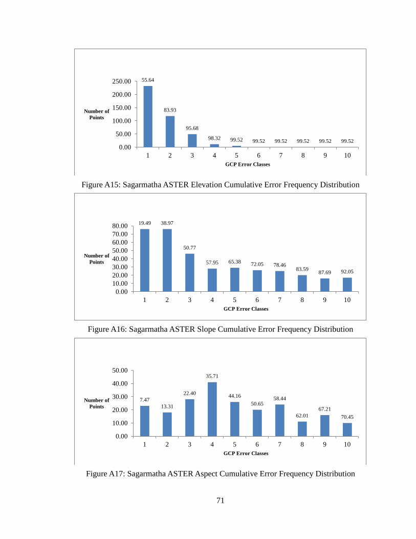
71

Figure A15: Sagarmatha ASTER Elevation Cumulative Error Frequency Distribution

Figure A16: Sagarmatha ASTER Slope Cumulative Error Frequency Distribution

Figure A17: Sagarmatha ASTER Aspect Cumulative Error Frequency Distribution

55.64

83.93

95.68

98.32 99.52 99.52 99.52 99.52 99.52 99.52 0.00

50.00

100.00

150.00

200.00

250.00

1 2 3 4 5 6 7 8 9 10

Number of Points

GCP Error Classes

Sagarmatha ASTER Elevation Cumulative Error Frequency Distribution

19.49 38.97

50.77

57.95 65.38 72.05 78.46 83.59 87.69 92.05

0.00 10.00 20.00 30.00 40.00 50.00 60.00 70.00 80.00

1 2 3 4 5 6 7 8 9 10

Number of Points

GCP Error Classes

Sagarmatha ASTER Slope Cumulative Error Frequency Distribution

7.47 13.31

22.40

35.71

44.16 50.65

58.44

62.01 67.21

70.45

0.00

10.00

20.00

30.00

40.00

50.00

1 2 3 4 5 6 7 8 9 10

Number of Points

GCP Error Classes

Sagarmatha ASTER Aspect Cumulative Error Frequency Distribution

72

APPENDIX B: SRTM Full-Class Cumulative Error Frequency Distribution

Figure B1: Annapurna SRTM Elevation Cumulative Error Frequency Distribution

Figure B2: Annapurna SRTM Slope Cumulative Error Frequency Distribution

0.00

20.00

40.00

60.00

80.00

100.00

1 2 3 4 5 6 7 8 9 10 11 12 13 14 15 16 17 18 19 20 21 22 23 24 25

Number of Points

GCP Error Classes

Annapurna SRTM Elevation Cumulative Error Frequency Distribution

0.00

5.00

10.00

15.00

20.00

25.00

1 2 3 4 5 6 7 8 9 10 11 12 13 14 15 16 17 18

Number of Points

GCP Error Classes

Annapurna SRTM Slope Cumulative Error Frequency Distribution

73

Figure B3: Annapurna SRTM Aspect Cumulative Error Frequency Distribution

Figure B4 Chitwan SRTM Elevation Cumulative Error Frequency Distribution

Figure B5 Chitwan SRTM Slope Cumulative Error Frequency Distribution

0.00

5.00

10.00

15.00

20.00

25.00

1 3 5 7 9 11 13 15 17 19 21 23 25 27 29 31 33 35

Number of Points

GCP Error Classes

Annapurna SRTM Aspect Cumulative Error Frequency Distribution

0.00 10.00 20.00 30.00 40.00 50.00 60.00 70.00 80.00

1 2 3 4 5 6 7 8 9 10 11 12 13 14 15 16 17 18 19 20 21 22 23 24 25

Number of Points

GCP Error Classes

Chitwan SRTM Elevation Cumulative Error Frequency Distribution

0.00

50.00

100.00

150.00

200.00

250.00

1 2 3 4 5 6 7 8 9 10 11 12 13 14 15 16 17 18

Number of Points

GCP Error Classes

Chitwan SRTM Slope Cumulative Error Frequency Distribution

74

Figure B6: Langtang SRTM Elevation Cumulative Error Frequency Distribution

Figure B7: Langtang SRTM Slope Cumulative Error Frequency Distribution

Figure B8: Langtang SRTM Aspect Cumulative Error Frequency Distribution

0.00

50.00

100.00

150.00

200.00

250.00

1 2 3 4 5 6 7 8 9 10 11 12 13 14 15 16 17 18 19 20 21 22 23 24 25

Number of Points

GCP Error Classes

Langtang SRTM Elevation Cumulative Error Frequency Distribution

0.00

5.00

10.00

15.00

20.00

25.00

30.00

1 2 3 4 5 6 7 8 9 10 11 12 13 14 15 16 17

Number of Points

GCP Error Classes

Langtang SRTM Slope Cumulative Error Frequency Distribution

0.00 2.00 4.00 6.00 8.00

10.00 12.00 14.00

1 3 5 7 9 11 13 15 17 19 21 23 25 27 29 31 33 35

Number of Points

GCP Error Classes

Langtang SRTM Aspect Cumulative Error Frequency Distribution

75

Figure B9: Makalu Barun SRTM Aspect Cumulative Error Frequency Distribution



0.00

10.00

20.00

30.00

40.00

50.00

60.00

1 2 3 4 5 6 7 8 9 10 11 12 13 14 15 16 17 18 19 20 21 22 23 24 25

Number of Points

GCP Error Classes

Makalu Barun SRTM Elevation Cumulative Error Frequency Distribution

0.00

10.00

20.00

30.00

40.00

50.00

60.00

1 2 3 4 5 6 7 8 9 10 11 12 13 14 15 16 17

Number of Points

GCP Error Classes

Makalu Barun SRTM Slope Cumulative Error Frequency Distribution

0.00

5.00

10.00

15.00

20.00

1 3 5 7 9 11 13 15 17 19 21 23 25 27 29 31 33 35

Number of Points

GCP Error Classes

Makalu Barun SRTM Aspect Cumulative Error Frequency Distribution

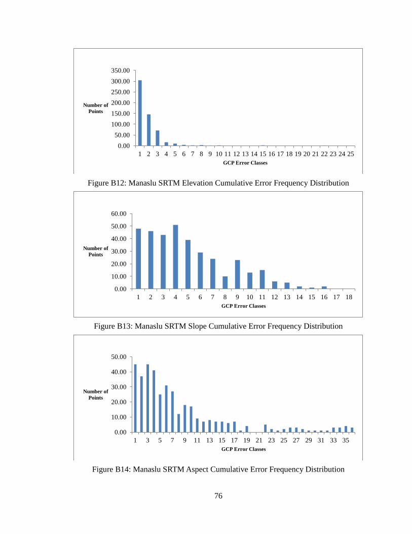
76

Figure B12: Manaslu SRTM Elevation Cumulative Error Frequency Distribution

Figure B13: Manaslu SRTM Slope Cumulative Error Frequency Distribution

Figure B14: Manaslu SRTM Aspect Cumulative Error Frequency Distribution

0.00 50.00

100.00 150.00 200.00 250.00 300.00 350.00

1 2 3 4 5 6 7 8 9 10 11 12 13 14 15 16 17 18 19 20 21 22 23 24 25

Number of Points

GCP Error Classes

Manaslu SRTM Elevation Cumulative Error Frequency Distribution

0.00

10.00

20.00

30.00

40.00

50.00

60.00

1 2 3 4 5 6 7 8 9 10 11 12 13 14 15 16 17 18

Number of Points

GCP Error Classes

Manaslu SRTM Slope Cumulative Error Frequency Distribution

0.00

10.00

20.00

30.00

40.00

50.00

1 3 5 7 9 11 13 15 17 19 21 23 25 27 29 31 33 35

Number of Points

GCP Error Classes

Manaslu SRTM Aspect Cumulative Error Frequency Distribution

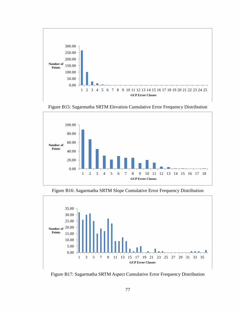
77

Figure B15: Sagarmatha SRTM Elevation Cumulative Error Frequency Distribution

Figure B16: Sagarmatha SRTM Slope Cumulative Error Frequency Distribution

Figure B17: Sagarmatha SRTM Aspect Cumulative Error Frequency Distribution

0.00

50.00

100.00

150.00

200.00

250.00

300.00

1 2 3 4 5 6 7 8 9 10 11 12 13 14 15 16 17 18 19 20 21 22 23 24 25

Number of Points

GCP Error Classes

Sagarmatha SRTM Elevation Cumulative Error Frequency Distribution

0.00

20.00

40.00

60.00

80.00

100.00

1 2 3 4 5 6 7 8 9 10 11 12 13 14 15 16 17 18

Number of Points

GCP Error Classes

Sagarmatha SRTM Slope Cumulative Error Frequency Distribution

0.00 5.00

10.00 15.00 20.00 25.00 30.00 35.00

1 3 5 7 9 11 13 15 17 19 21 23 25 27 29 31 33 35

Number of Points

GCP Error Classes

Sagarmatha SRTM Aspect Cumulative Error Frequency Distribution

78

APPENDIX C: ASTER Full-Class Cumulative Error Frequency Distribution

Figure C1: Annapurna ASTER Elevation Cumulative Error Frequency Distribution

Figure C2: Annapurna ASTER Slope Cumulative Error Frequency Distribution

0.00

20.00

40.00

60.00

80.00

100.00

1 2 3 4 5 6 7 8 9 10 11 12 13 14 15 16 17 18 19 20 21 22 23 24 25

Number of Points

GCP Error Classes

Annapurna ASTER Elevation Cumulative Error Frequency Distribution

0.00 5.00

10.00 15.00 20.00 25.00 30.00 35.00

1 2 3 4 5 6 7 8 9 10 11 12 13 14 15 16 17 18

Number of Points

GCP Error Classes

Annapurna ASTER Slope Cumulative Frequency Error Distribution

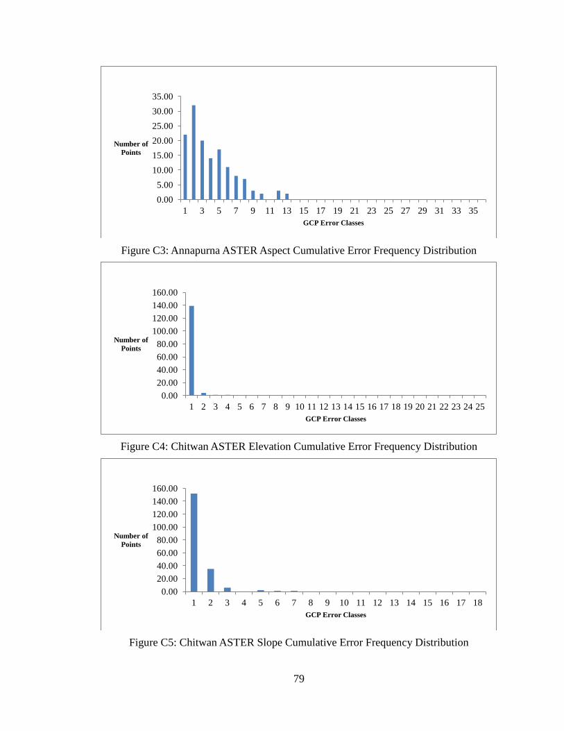
79

Figure C3: Annapurna ASTER Aspect Cumulative Error Frequency Distribution

Figure C4: Chitwan ASTER Elevation Cumulative Error Frequency Distribution

Figure C5: Chitwan ASTER Slope Cumulative Error Frequency Distribution

0.00 5.00

10.00 15.00 20.00 25.00 30.00 35.00

1 3 5 7 9 11 13 15 17 19 21 23 25 27 29 31 33 35

Number of Points

GCP Error Classes

Annapurna ASTER Aspect Cumulative Error Frequency Distribution

0.00 20.00 40.00 60.00 80.00

100.00 120.00 140.00 160.00

1 2 3 4 5 6 7 8 9 10 11 12 13 14 15 16 17 18 19 20 21 22 23 24 25

Number of Points

GCP Error Classes

Chitwan ASTER Elevation Cumulative Error Frequency Distribution

0.00 20.00 40.00 60.00 80.00

100.00 120.00 140.00 160.00

1 2 3 4 5 6 7 8 9 10 11 12 13 14 15 16 17 18

Number of Points

GCP Error Classes

Chitwan ASTER Slope Cumulative Error Frequency Distribution

80

Figure C6: Langtang ASTER Elevation Cumulative Error Frequency Distribution

Figure C7: Langtang ASTER Slope Cumulative Error Frequency Distribution

Figure C8: Langtang ASTER Aspect Cumulative Error Frequency Distribution

0.00

50.00

100.00

150.00

200.00

250.00

1 2 3 4 5 6 7 8 9 10 11 12 13 14 15 16 17 18 19 20 21 22 23 24 25

Number of Points

GCP Error Classes

Langtang ASTER Elevation Cumulative Error Frequency Distribution

0.00

5.00

10.00

15.00

20.00

25.00

1 2 3 4 5 6 7 8 9 10 11 12 13 14 15 16 17

Number of Points

GCP Error Classes

Langtang ASTER Slope Cumulative Error Frequency Distribution

0.00 2.00 4.00 6.00 8.00

10.00 12.00 14.00

1 3 5 7 9 11 13 15 17 19 21 23 25 27 29 31 33 35

Number of Points

GCP Error Classes

Langtang ASTER Aspect Cumulative Error Frequency Distribution

81

Figure C9: Makalu Barun ASTER Elevation Cumulative Error Frequency Distribution

Figure C10: Makalu Barun ASTER Slope Cumulative Error Frequency Distribution

Figure C11: Makalu Barun ASTER Aspect Cumulative Error Frequency Distribution

0.00

10.00

20.00

30.00

40.00

50.00

1 2 3 4 5 6 7 8 9 10 11 12 13 14 15 16 17 18 19 20 21 22 23 24 25

Number of Points

GCP Error Classes

Makalu Barun ASTER Elevation Cumulative Error Frequency Distribution

0.00

10.00

20.00

30.00

40.00

50.00

1 2 3 4 5 6 7 8 9 10 11 12 13 14 15 16 17

Number of Points

GCP Error Classes

Makalu Barun ASTER Slope Cumulative Error Frequency Distribution

0.00

5.00

10.00

15.00

20.00

25.00

30.00

1 3 5 7 9 11 13 15 17 19 21 23 25 27 29 31 33 35

Number of Points

GCP Error Classes

Makalu Barun ASTER Aspect Cumulative Error Frequency Distribution

82

Figure C12: Manaslu ASTER Elevation Cumulative Error Frequency Distribution

Figure C13: Manaslu ASTER Slope Cumulative Error Frequency Distribution

Figure C14: Manaslu ASTER Aspect Cumulative Error Frequency Distribution

0.00 50.00

100.00 150.00 200.00 250.00 300.00 350.00

1 2 3 4 5 6 7 8 9 10 11 12 13 14 15 16 17 18 19 20 21 22 23 24 25

Number of Points

GCP Error Classes

Manaslu ASTER Elevation Cumulative Error Frequency Distribution

0.00

10.00

20.00

30.00

40.00

50.00

60.00

1 2 3 4 5 6 7 8 9 10 11 12 13 14 15 16 17 18

Number of Points

GCP Error Classes

Manaslu ASTER Slope Cumulative Error Frequency Distribution

0.00 5.00

10.00 15.00 20.00 25.00 30.00 35.00 40.00 45.00

1 3 5 7 9 11 13 15 17 19 21 23 25 27 29 31 33 35

Number of Points

GCP Error Classes

Manaslu ASTER Aspect Cumulative Error Frequency Distribution

83

Figure C15: Sagarmatha ASTER Elevation Cumulative Error Frequency Distribution

Figure C16: Sagarmatha ASTER Slope Cumulative Error Frequency Distribution

Figure C17: Sagarmatha ASTER Aspect Cumulative Error Frequency Distribution

0.00

50.00

100.00

150.00

200.00

250.00

1 2 3 4 5 6 7 8 9 10 11 12 13 14 15 16 17 18 19 20 21 22 23 24 25

Number of Points

GCP Error Classes

Sagarmatha ASTER Elevation Cumulative Error Frequency Distribution

0.00 10.00 20.00 30.00 40.00 50.00 60.00 70.00 80.00

1 2 3 4 5 6 7 8 9 10 11 12 13 14 15 16 17 18

Number of Points

GCP Error Classes

Sagarmatha ASTER Slope Cumulative Error Frequency Distribution

0.00 5.00

10.00 15.00 20.00 25.00 30.00 35.00 40.00 45.00

1 3 5 7 9 11 13 15 17 19 21 23 25 27 29 31 33 35

Number of Points

GCP Error Classes

Sagarmatha ASTER Aspect Cumulative Error Frequency Distribution

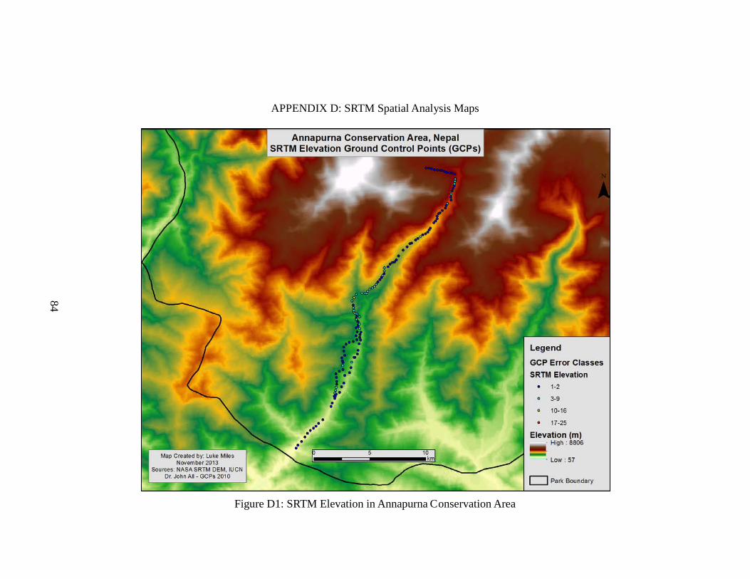
84

APPENDIX D: SRTM Spatial Analysis Maps

Figure D1: SRTM Elevation in Annapurna Conservation Area

85

Figure D2: SRTM Slope in Annapurna Conservation Area

86

Figure D3: SRTM Aspect in Annapurna Conservation Area

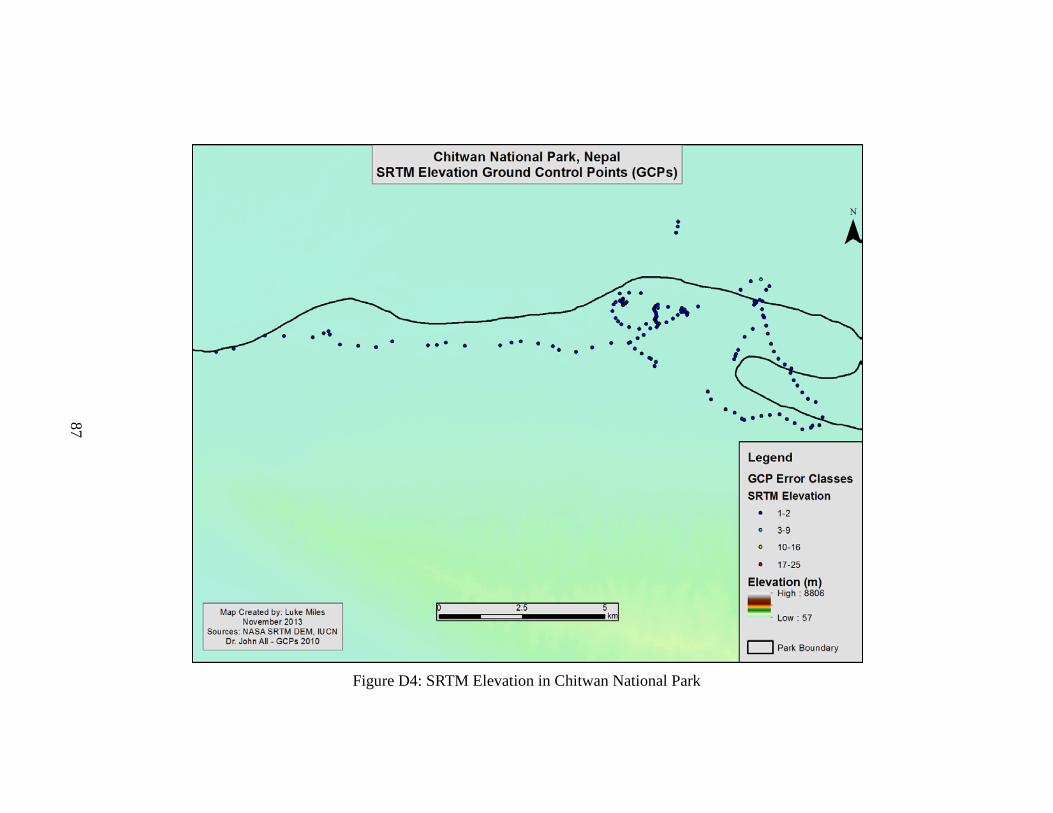
87

Figure D4: SRTM Elevation in Chitwan National Park

88

Figure D5: SRTM Slope in Chitwan National Park

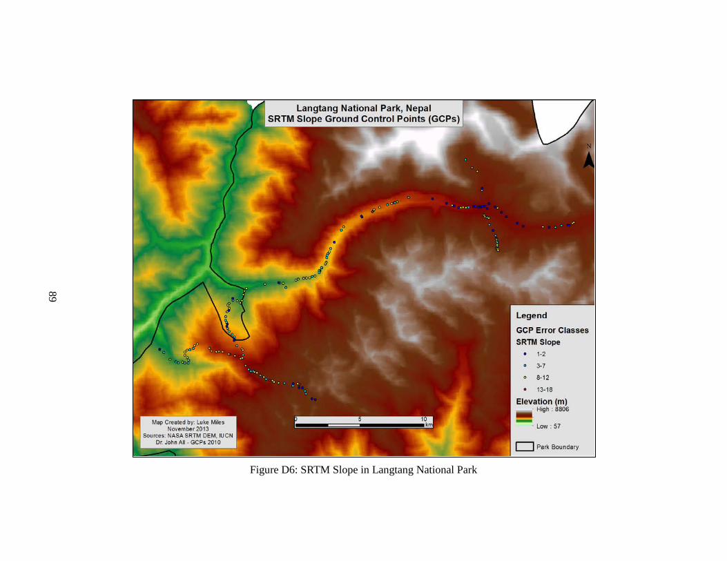
89

Figure D6: SRTM Slope in Langtang National Park

90

Figure D7: SRTM Aspect in Langtang National Park

91

Figure D8: SRTM Slope in Makalu Barun National Park

92

Figure D9: SRTM Aspect in Makalu Barun National Park

93

Figure D10: SRTM Elevation in Manaslu Conservation Area

94

Figure D11: SRTM Slope in Manaslu Conservation Area

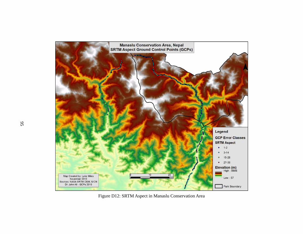
95

Figure D12: SRTM Aspect in Manaslu Conservation Area

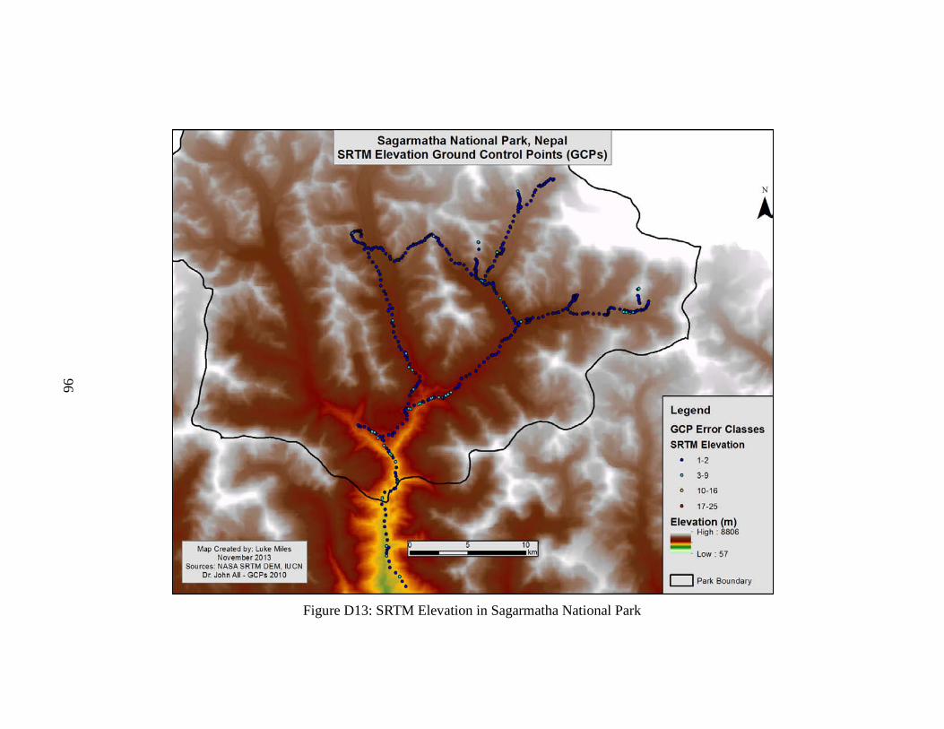
96

Figure D13: SRTM Elevation in Sagarmatha National Park

97

Figure D14: SRTM Slope in Sagarmatha National Park

98

Figure D15: SRTM Aspect in Sagarmatha National Park

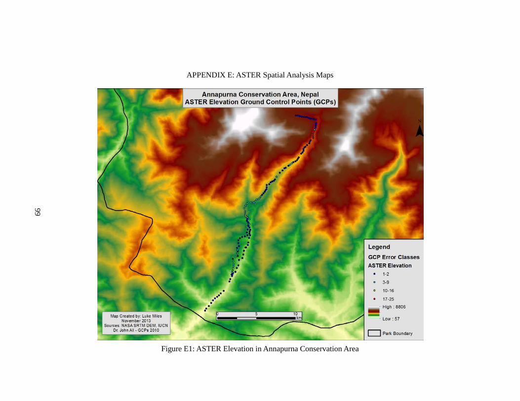
99

APPENDIX E: ASTER Spatial Analysis Maps

Figure E1: ASTER Elevation in Annapurna Conservation Area

100

Figure E2: ASTER Slope in Annapurna Conservation Area

101

Figure E3: ASTER Elevation in Chitwan National Park

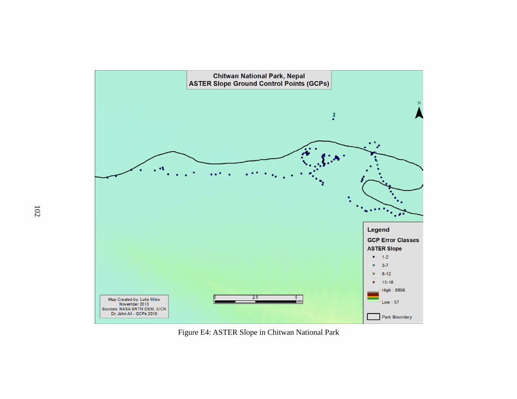
102

Figure E4: ASTER Slope in Chitwan National Park

103

Figure E5: ASTER Elevation in Langtang National Park

104

Figure E6: ASTER Aspect in Langtang National Park

105

Figure E7: ASTER Elevation in Makalu Barun National Park

106

Figure E8: ASTER Slope in Makalu Barun National Park

107

Figure E9: ASTER Elevation in Manaslu Conservation Area

108

Figure E10: ASTER Slope in Manaslu Conservation Area

109

Figure E11: ASTER Aspect in Manaslu Conservation Area

110

Figure E12: ASTER Elevation in Sagarmatha National Park

111

Figure E13: ASTER Aspect in Sagarmatha National Park

112

BIBLIOGRAPHY Aniello, P. (2003). Using ASTER DEMS to produce IKONOS orthophotos. Earth

Observation Magazine, 12(5), 22-26.

Aryal, A. (2005). Status and distribution of Himalayan Musk deer ‘Moschus

chrysogaster’ in Annapurna Conservation Area of Manang District, Nepal. UK:

ITNC. Retrieved on September 14, 2013, from

www.itnc.org/FinalReportonMuskdeerManang.pdf.

Bajimaya, S. (2003). Nepal’s experience in participatory biodiversity conservation with

emphasis on buffer zone initiatives. Policy Matters. Section I: The complexities of

governing protected areas, 12, 276-282.

Bajracharya, B., and Uddin, K. (2010). Study of Land Cover Dynamics in Sagarmatha

National Park and Buffer Zone. In Kaufman V. (ed.), Proceedings of the 10th

International Symposium on High Mountain Remote Sensing Cartography,

Kathmandu, Nepal, September 8-11, 2008, 125-132, Graz, Austria: Institute of

Geography and Regional Science, Karl-Franzens-University of Graz, 2010.

Baral, N., Stern, M.J., Heinen, J.T., 2007a. Integrated conservation and development

Project life cycles in the Annapurna Conservation Area, Nepal: is development

overpowering conservation? Biodiversity and Conservation, 16, 2903-2917.

Becker, A., Körner, C., Brun, J. J., Guisan, A., and Tappeiner, U. (2007). Ecological and

land use studies along elevational gradients. Mountain Research and

Development, 27(1), 58-65.

Beniston, M. (2003). Climatic change in mountain regions: a review of possible impacts.

Climatic Change, 59, 5-31.

113

Bennie, J., Hill, M. O., Baxter, R., and Huntley, B. (2006). Influence of slope and aspect

on long‐term vegetation change in British chalk grasslands. Journal of Ecology,

94(2), 355-368.

Berthier, E., Vadon, H., Baratoux, D., Arnaud, Y., Vincent, C., Feigl, K. L., Rémy, F.,

and Légresy, B. (2005). Surface motion of mountain glaciers derived from

satellite optical imagery. Remote Sensing of Environment, 95(1), 14-28.

Berthier, E., Arnaud, Y., Vincent, C., and Rémy, F. (2006). Biases of SRTM in high-

mountain areas: Implications for the monitoring of glacier volume changes,

Geophysical Research Letters, 33(8). L08502, doi:10.1029/2006GL025862.

Bhattarai, K. R., and Vetaas, O. R. (2003). Variation in plant species richness of different

life forms along a subtropical elevation gradient in the Himalayas, east

Nepal. Global Ecology and Biogeography, 12(4), 327-340.

Bhuju, U. R., Shakya, P. R., Basnet, T. B., and Shrestha, S. (2007). Nepal Biodiversity

Resource Book: Protected Areas, Ramsar Sites, and World Heritage Sites.

Kathmandu, Nepal: United Nations Environment Programme (UNEP); Ministry

of Environment, Science and Technology, Government of Nepal (MoEST).

Bhusal, N. P. (2009). Chitwan National Park: A Prime Destination of Eco-Tourism in

Central Tarai Region, Nepal. The Third Pole: Journal of Geography Education, 5,

70-75.

Bolch, T., Kamp, U., and Olsenholler, J. (2005). Using ASTER and SRTM DEMs for

studying geomorphology and glaciation in high mountain areas. In Oluic M. (ed.)

New Strategies for European Remote Sensing, Rotterdam, Netherlands: Millpress,

119-127.

114

Byers, A. (2005). Contemporary human impacts on Alpine ecosystems in the Sagarmatha

(Mt. Everest) national park, Khumbu, Nepal. Annals of the Association of

American Geographers, 95(1), 112-140.

Byers, A. (2009). A comparative study of tourism impacts on alpine ecosystems in the

Sagarmatha (Mt. Everest) National Park, Nepal and the Huascaran National Park,

Peru. In: Hill, J. and Gale, T. (eds.), Ecotourism and Environmental

Sustainability: Principle and Practice. Burlington, VT: Ashgate Publishing Ltd.,

51–72.

Carson, M. A. (1969). Models of hillslope development under mass failure. Geographical

Analysis, 1(1), 76-100.

CGIAR-CSI (Consultive Group on International Agricultural Research - Consortium for

Spatial Information). (2013). CGIAR-CSI. Retrieved December 3, 2013, from

http://www.cgiar-csi.org/data/srtm-90m-digital-elevation-database-v4-1.

Chakraborty, R. N. (2001). Stability and outcomes of common property institutions in

forestry: evidence from the Terai region of Nepal. Ecological Economics, 36(2),

341-353.

Chang, K. T. (2010). Introduction to Geographic Information Systems. New York, NY:

McGraw-Hill.

Cooper, M. A. R. (1998). Datums, coordinates and differences. In Lane, S., Richards, K.,

and Chandler, J. (ed.), Landform Monitoring, Modelling and Analysis, Chichester:

Wiley, 21-36.

115

Corchete, V., Flores, D., and Oviedo, F. (2006). The first high-resolution gravimetric

geoid for the Bolivian tableland: BOLGEO. Physics of the Earth and Planetary

Interiors, 157(3), 250-256.

Eiumnoh, A., and Shrestha, R. P. (2000). Application of DEM data to Landsat image

classification: Evaluation in a tropical wet-dry landscape of Thailand.

Photogrammetric Engineering and Remote Sensing, 66(3), 297-304.

Farr, T. G., Rosen, P. A., Caro, E., Crippen, R., Duren, R., Hensley, S., ... and Alsdorf, D.

(2007). The shuttle radar topography mission. Reviews of Geophysics, 45(2),

RG2004, doi:10.1029/2005RG000183.

Goncalves, J., and Fernandes, J. C. (2005, June). Assessment of SRTM-3 DEM in

Portugal with topographic map data. Proceedings of the EARSeL Workshop 3D-

Remote Sensing, Porto, Portugal.

Gorokhovich, Y., and Voustianiouk, A. (2006). Accuracy assessment of the processed

SRTM-based elevation data by CGIAR using field data from USA and Thailand

and its relation to the terrain characteristics. Remote Sensing of Environment, 104,

409−415.

Gurung, B., Smith, J. L. D., McDougal, C., Karki, J. B., and Barlow, A. (2008). Factors

associated with human-killing tigers in Chitwan National Park, Nepal. Biological

Conservation, 141(12), 3069-3078.

Gurung, J., and Bajracharya, R. M. (2012). Climate change and glacial retreat in the

Himalaya: implications for soil and plant development. Kathmandu University

Journal of Science, Engineering and Technology, 8(1), 153-163.

116

Hale, S. R., and Rock, B. N. (2003). Impact of topographic normalization on land-cover

classification accuracy. Photogrammetric Engineering and Remote

Sensing, 69(7), 785-792.

Heipke, C. (1999). Digital photogrammetric workstations. GIM International, 1, 81.

Hirano, A., Welch, R., and Lang, H. (2003). Mapping from ASTER stereo image data:

DEM validation and accuracy assessment. ISPRS Journal of Photogrammetry and

Remote Sensing, 57(5), 356-370.

Hofton, M., Dubayah, R., Blair, J. B., and Rabine, D. (2006). Validation of SRTM

elevations over vegetated and non-vegetated terrain using medium footprint lidar.

Photogrammetric Engineering and Remote Sensing, 72(3), 279-285.

Holmes, K. W., Chadwick, O. A., and Kyriakidis, P. C. (2000). Error in a USGS 30-meter

digital elevation model and its impact on terrain modeling. Journal of Hydrology,

233(1), 154-173.

Huggel, C., Caplan-Auerbach, J., Waythomas, C. F., and Wessels, R. L. (2007).

Monitoring and modeling ice-rock avalanches from ice-capped volcanoes: A case

study of frequent large avalanches on Iliamna Volcano, Alaska. Journal of

Volcanology and Geothermal Research, 168(1), 114-136.

Huggel, C., Schneider, D., Miranda, P. J., Delgado Granados, H., and Kääb, A. (2008).

Evaluation of ASTER and SRTM DEM data for lahar modeling: a case study on

lahars from Popocatépetl Volcano, Mexico. Journal of Volcanology and

Geothermal Research, 170(1), 99-110.

IUCN (International Union for Conservation of Nature). (2013). IUCN. Retrieved

December 3, 2013, from http://www.iucn.org.

117

Jensen, J.R. (2005). Introductory Digital Image Processing: A Remote Sensing

Perspective (3rd ed.). Upper Saddle River, NJ: Prentice Hall.

Kääb, A., Huggel, C., Paul, F., Wessels, R., Raup, B., Kieffer, H., and Kargel, J. (2002,

March). Glacier monitoring from ASTER imagery: accuracy and applications.

Proceedings of EARSeL-LISSIG-Workshop Observing our Cryosphere from

Space, Bern, Switzerland, EARSeL eProceedings, 2, 43-53.

Kääb, A. (2005). Combination of SRTM3 and repeat ASTER data for deriving alpine

glacier flow velocities in the Bhutan Himalaya. Remote Sensing of Environment,

94(4), 463-474.

Khadka, D., and Nepal, S. K. (2010). Local responses to participatory conservation in

Annapurna Conservation Area, Nepal. Environmental Management, 45(2), 351-

362.

Kottek, M., Grieser, J., Beck, C., Rudolf, B., & Rubel, F. (2006). World map of the

Koppen-Geiger climate classification updated. Meteorologische Zeitschrift, 15(3),

259-264.

Lambin, E. F., and Geist, H. J. (2006). Land Use and Land Cover Change: Local

Processes and Global Impacts. Berlin, Germany: Springer Verlag.

Liu, J. G., Mason, P. J., Clerici, N., Chen, S., Davis, A., Miao, F., ... and Liang, L.

(2004). Landslide hazard assessment in the Three Gorges area of the Yangtze

river using ASTER imagery: Zigui–Badong. Geomorphology, 61(1), 171-187.

Liu, Y. (2008). An evaluation on the data quality of SRTM at the alpine and plateau,

North-Western of China. The International Archives of the Photogrammetry,

Remote Sensing and Spatial Information Sciences, 37(1), 1123-1128.

118

Liverman, D. (2004). Who governs, at what scale and at what price? Geography,

environmental governance, and the commodification of nature. Annals of the

Association of American Geographers, 94(4), 734-738.

Mahal, B. (1988). National parks and local development: grasses and people in Royal

Chitwan National Park, Nepal. Environmental Conservation, 15(2), 143-148.

Manguard, S. (2010). [Inset of Himalaya Mountain Range]. Retrieved from

http://en.wikipedia.org/wiki/File:Himalayas_Map.png.

METI (Ministry of Economy, Trade and Industry). (2012). ASTER Global Digital

Elevation Model (GDEM). Retrieved November 29, 2012, from

http://www.jspacesystems.or.jp/ersdac/GDEM/E/2.html.

Mishra, H. R., McNeely, J. A., and Miller, K. R. (1985). A delicate balance: tigers,

rhinoceros, tourists and park management vs. the needs of the local people in

Royal Chitwan National Park, Nepal. National parks, conservation, and

development. The role of protected areas in sustaining society. Proceedings of the

World Congress on National Parks, Bali, Indonesia, 11-12 October 1982, 197-

205. Washington, DC: Smithsonian Institution Press.

Mishra, P. N. (2003). The Langtang National Park: A proposed first biosphere reserve in

Nepal. Journal of the National Science Foundation of Sri Lanka, 31(1-2), 333-

335.

Mugnier, J. L., Leturmy, P., Mascle, G., Huyghe, P., Chalaron, E., Vidal, G., ... and

Delcaillau, B. (1999). The Siwaliks of western Nepal: I. Geometry and

kinematics. Journal of Asian Earth Sciences, 17(5), 629-642.

119

NASA (National Aeronautics and Space Administration) Global Digital Elevation Model

Project. (2013). NASA Global Digital Elevation Model Project. Retrieved

December 3, 2013, from http://asterweb.jpl.nasa.gov/gdem.asp.

NASA SRTM DEM (National Aeronautics and Space Administration Shuttle Radar

Topography Mission Digital Elevation Model). (2011). NASA Shuttle Radar

Topography Mission. Retrieved February 15, 2011, from

http://www2.jpl.nasa.gov/srtm/.

Nepal, S. K., and Weber, K. E. (1995). The quandary of local people—Park relations in

Nepal's Royal Chitwan National Park. Environmental Management, 19(6), 853-

866.

Nikolakopoulos, K. G. and Chrysoulakis, N. (2006). Updating the 1:50.000 topographic

maps using ASTER and SRTM DEM: The case of Athens, Greece. In Ehlers M.

and Michel U. (eds.) Remote Sensing for Environmental Monitoring, GIS

Applications, and Geology VI, Proceedings of SPIE 6366, doi:10.1117/12.689016.

NTNC (National Trust for Nature Conservation). (2013). Annapurna Conservation Area

Project. Retrieved November 5, 2013, from

http://www.ntnc.org.np/project/annapurna-conservation-area-project.

Rabus, B., Eineder, M., Roth, A., and Bamler, R. (2003). The shuttle radar topography

mission—a new class of digital elevation models acquired by spaceborne radar.

ISPRS Journal of Photogrammetry and Remote Sensing, 57(4), 241-262.

Rodriguez, E., Morris, C. S., and Belz, J. E. (2006). A global assessment of the SRTM

performance. Photogrammetric Engineering and Remote Sensing, 72(3), 249-260.

120

Saha, A.K., Arora, M.K., Csaplovics, E. and Gupta, R.P., (2005), Land cover

classification using IRS LISS III imagery and DEM in a rugged terrain: A case

study in Himalaya. GeoCarto International, 20(2), 33–40.

Sanyal, J., and Lu, X. X. (2005). Remote sensing and GIS‐based flood vulnerability

assessment of human settlements: a case study of Gangetic West Bengal, India.

Hydrological Processes, 19(18), 3699-3716.

Schowengerdt, R. A. (2007). Remote Sensing Models and Methods for Image Processing

(3rd ed.). Burlington, MA: Academic Press.

Sesnie, S.E., Hagell, S.E., Otterstom, S.M., Chambers, C.L., and Dickson, B.G. (2008).

STRM-DEM and Landsat ETM+ data for mapping tropical dry forest cover and

biodiversity assessment in Nicaragua. Revista Geográfica Académica, 2(2), 53–

65.

Sharma K., Saraf, A.K., Das J.D., Rawat, V., and Shujat, Y. (2010). SRTM and ASTER

DEM characteristics of two areas from Himalayan region. International

Geoinformatics Research and Development Journal, 1(3), 25-31.

Shrestha, K. L. (2005). Global change impact assessment for Himalayan mountain

regions for environmental management and sustainable development. Global

Environmental Research, 9(1), 69-81.

Singh, K., Maikhuri, R. K., Rao, K. S., and Saxena, K. G. (2008). Characterizing land-

use diversity in village landscapes for sustainable mountain development: a case

study from Indian Himalaya. The Environmentalist, 28(4), 429-445.

121

Srivastava, B. K., and Ramalingam, K. (2006). Error estimates for WGS-84 and Everest

(India-1956) transformation. GIS Development. Retrieved November 8, 2013,

from http://www.gisdevelopment.net/technology/ip/ma03037.htm.

SRTM (Shuttle Radar Topography Mission). (2013). Interferometric Synthetic Aperture

Radar (IFSAR) Shuttle Radar Topography Mission (SRTM). Retrieved November

23, 2013, from http://www.fas.org/irp/program/collect/ifsar.htm.

Tralli, D.M., Blom, R.G., Zlotnicki, V., Donnellan, A., Evans, D.L. (2005). Satellite

remote sensing of earthquake, volcano, flood, landslide and coastal inundation

hazards. ISPRS Journal of Photogrammetry and Remote Sensing 59(4): 185–198.

Tulu, M. D. (2005). SRTM DEM Suitability in Runoff Studies. Master of Science Thesis.

International Institute for Geo-information and Earth Observation. The

Netherlands.

USGS (United States Geological Survey). (2013). The Himalayas [This Dynamic Earth].

Retrieved November 5, 2013, from

http://pubs.usgs.gov/gip/dynamic/himalaya.html.

Ustun, A., Bildirici, I.O.., Selvi, H.Z., Abbak, R.A. (2006, January) An evaluation of

SRTM3 DTM data: Validity, problems and solutions, The first international

conference on cartography and GIS, Borovets, Bulgaria.

Van Niel, T. G., McVicar, T.R., Li L.T., Gallant, J.C., and Yang, Q.K. (2008). The impact

of misregistration on SRTM and DEM image differences. Remote Sensing of

Environment, 112(5), 2430–2442.

Whiteman, C. D. (2000). Mountain Meteorology: Fundamentals and Applications. New

York, NY: Oxford University Press.

122

Xu, J., Grumbine, R. E., Shrestha, A., Eriksson, M., Yang, X., Wang, Y. U. N., and

Wilkes, A. (2009). The melting Himalayas: cascading effects of climate change

on water, biodiversity, and livelihoods. Conservation Biology, 23(3), 520-530.

Yamaguchi, Y., Kahle, A. B., Tsu, H., Kawakami, T., and Pniel, M. (1998). Overview of

advanced spaceborne thermal emission and reflection radiometer (ASTER). IEEE

Transactions on Geoscience and Remote Sensing, 36(4), 1062-1071.

Yang, Q., and Zheng, D. (2004). Tibetan Geography. Beijing, China: China

Intercontinental Press.

Zomer, R. J., Ustin, S. L., and Carpenter, C. C. (2001). Land cover change along tropical

and subtropical riparian corridors within the Makalu Barun National Park and

Conservation Area, Nepal. Mountain Research and Development, 21(2), 175-183.

Zomer, R., Ustin, S., and Ives, J. (2002). Using satellite remote sensing for DEM

extraction in complex mountainous terrain: landscape analysis of the Makalu

Barun National Park of eastern Nepal. International Journal of Remote Sensing,

23(1), 125-143.

global digital elevation model accuracy assessment in the

Documents