1

Global economic crisis, gender and poverty in the Philippines

Erwin Corong1

1. Introduction

The 2008-09 global economic contraction has brought renewed concerns regarding

economic security and welfare in the developing world. This is because although developing

countries may be affected differently—owing to their heterogeneity and varying linkage to the

global economy—fears of possible reversals of economic progress, susceptibility to greater

instability and higher risk have been expressed (Lin 2008). Indeed, apart from the projected short-

term financing requirement of about $270 to $700 billion dollars—not to mention a myriad of

negative economic effects—developing countries also confront the possibility of facing a higher

spread on their own issued sovereign bonds in the long term.

Whereas global economic activity is expected to recover by 2010, the rebound is projected

to be sluggish and may not be enough to counter the rise in unemployment and poverty levels that

the global contraction has additionally inflicted (IMF 2009). Estimates confirm that a significant

number of people have been affected. The International labour organization (ILO 2009) reported a

reduction in global employment of 1.4 percent in 2008 and expects additional unemployment to

increase between 39 and 59 million people in 2009. Chen and Ravallion (2009) estimate that

because of the crisis, 64 million people have additionally fallen into poverty based on $2 a day

poverty line. More importantly, the crisis is expected not only to slow down the progress of

achieving the Millennium Development Goals (MDGs) for developing countries, but also increase the

cost of achieving them. For instance in Latin America, countries must additionally spend about 1.5 to

2 percent of GDP per year between 2010 and 2015 in order to meet their MDGs (Sanchez and Vos

2009).

The Philippines like most developing economies has not been spared from the global

economic contraction. Although the country’s financial sector remained stable, owing to reforms

1 Phd student, Centre of Policy Studies (CoPS), Monash University. Funding from the Poverty and Economic Policy (PEP) research network

is acknowledged. PEP is financed by the Australian Agency for International Development (AusAid) and the government of Canada through

the International Development Research Centre (IDRC) and Canadian International Development Agency (CIDA).

.

2

instituted after the 1997 Asian financial crisis and limited exposure to US assets, it still suffered a

dramatic deceleration in economic growth. This deceleration is attributed to slowdown in

international trade, reduction foreign direct investment, cutback in household consumption and

moderate increase in unemployment (Yap et al. 2009).

The evidence so far suggests that export demand and investment are the two principal

channels with which the global economic contraction has affected the Philippine economy. Weak

global demand resulted in Philippine exports falling dramatically by 25 percent in July 2009 or a fall

of roughly US$1 billion dollars in export earnings when compared to the same period in 2008.

Electronic products which account for almost 57 percent of total Philippine export revenue fell by 26

percent resulting in foregone export earnings of about US$600 million dollars in 2008. Moreover, 8

out of 10 key exports earners registered a significant reduction ranging from 14 percent in wiring

products to as high as 65 percent reduction in copper exports. Foreign direct investments to the

Philippines also contracted due to uncertainty and risk aversion, compounded by the fact that the

United States is the biggest investor in the country. In 2008, net foreign direct investments from

January to November stood at US$1.7 billion dollars, roughly 41 percent below 2007 levels, whereas

net inflow of equity capital in 2008 reached US$1 billion dollars, which is 50 percent less than those

obtained in 2007 (Diokno 2008). Fortunately, remittance from Overseas Filipino workers (OFWs),

which accounts for about 10 percent of the Gross National Product (GNP), remained buoyant albeit

growing at a marginal 3 percent relative to 2008 levels (BSP 2009)—since a majority of OFWs are

working in the Middle East.

Analyses based on a community based monitoring system (CMBS) household survey—which was

conducted on a sample of 2082 households to capture the impact of the crisis on Filipino households in

2009—reveals that households have been affected by changes in both domestic and international

environment (Reyes et al. 2009). Out of 415 households with a household member working abroad: 16

percent had a member who was retrenched and has since gone back to the country; and 9 percent

reported a fall in remittances received owing to a wage reduction experienced by the household member

working abroad. On the domestic front and based on the full sample of households: 2.8 percent reported

having members experienced a reduction in wages; 2.2 confirmed that members working hours have been

reduced; and less than a percent reported a reduction in benefits. Some households have likewise

reported that a member has been laid off while others saw a reduction or a cessation in their

entrepreneurial activity.

While recent assessments on the impact of global crisis on the Philippines have been made (cf.

Diokno 2008; Yap et al. 2009; Reyes et al. 2009), no study has so far assessed the economy-wide effects

and the poverty and inequality impacts of the crisis on the Philippine economy. Furthermore, no analysis

3

has been undertaken to understand how the crisis may have affected women and gender in the

Philippines. To the extent that most women in the Philippines work in export-oriented industries such as

textiles and semi-conductors, as well as in service related industries like trade and business process

outsourcing, it is important that an analysis that accounts for the differential impact on men and women

be undertaken. Indeed, past experience confirm that as a result of the 1997 Asian financial crisis, women

labor market participation and working hours have increased relative to men.

Using a computable general equilibrium model linked to a micro-simulation module, this paper

analyzes the economy-wide effects of a reduction in export demand facing the Philippine economy.

We pay particular emphasis on the exports channel relative to the foreign direct investment (FDI)

since investment inflows into the Philippines declined since the turn of the century. Hence, FDI has

not been a significant source of economic growth unlike the country’s East Asian neighbors. The

analysis traces the transmission channels from the macro-economic to the microeconomic level: from

gross domestic product to output and factor supplies and demands; from commodity and factor prices

to employment by gender and household incomes to levels of poverty and income distribution.

The remaining sections are organized as follows: Section 2 describes the database while

section 3 describes the model. Section 4 enumerates the simulations, describes the mechanism

employed to capture reduction in export demand volume facing the Philippines, and analyzes the

simulation results. Section 5 concludes and provides suggestions for further research.

2. The Database

This section explains the database and describes the economic structure of the

Philippine economy based on the year 2000 input–output table (I-O), labor force survey

(LFS) and the family income and expenditure survey (FIES). Figure 1 presents the schematic

representation of the database, which reveals an absorption matrix showing detailed

purchases made by agents in the economy. Each economic agent/demander corresponds to a

column vector while each row vector distinguishes the type of outlay incurred. Agents are

classified into industries, investments, households, exports, government, and inventories;

outlays are categorized into basic flows (commodities by sources at basic prices), margins,

taxes, labor, capital, land, production tax and other costs.

Figure 1: Schematic representation of the Database

4

Absorption Matrix

1 2 3 4 5 6

Producers

Investors

Household

Export

Other

Change in

Inventories

Size I I H 1 1 1

Basic Flows

CS

V1BAS

V2BAS

V3BAS

V4BAS

V5BAS

V6BAS

Margins

CSM

V1MAR

V2MAR

V3MAR

V4MAR

V5MAR

n/a

Taxes

CS

V1TAX

V2TAX

V3TAX

V4TAX

V5TAX

n/a

Labor

O

V1LAB

Capital

1

V1CAP

C = 35 commodities

I = 35 industries

Land

1

V1LND

S = 2 sources: domestic and imported

O = 6 occupation types

Other Costs 1

V1OCT

M = 3 commodities used as margins.

H = 42,094 household

Source: Adapted from Horridge (2007)

The dimension of the database is determined by the number of industries (I),

commodities (C), sources (S), margin commodities (M), occupation types (O) and households

(H). In this application, there are 35 industries and commodities, 2 sources, 3 margins

services, 6 occupation types classified by skill and gender, and all 42,094 from the household

survey. Each of the C commodities can be obtained from two sources S, either locally or

imported from abroad. M of the domestically produced goods is also classified as margin

commodities, which are responsible for transferring commodities from their sources to their

users.

A salient feature of this database is its ease of reference—the different outlays are

additionally identified by a three letter acronym, and agents correspondingly represent a

number based on the column they occupy. Thus, each cell in the absorption matrix names the

corresponding data matrix and these names follow a pattern. For example, V1BAS, which

lies at the intersection of the first column and first row, is a 3-dimensional array showing the

cost of commodity flows from sources S to producers. Similarly, V1MAR, the intersection of

the first column and second row, is a 4-dimensional array showing the value of margin

services type M used to deliver each basic flow of good C, from sources S, to investors.

Let us now explore the individual sub-matrices found in the database. The first row

5

termed ―BAS‖, with dimension CxS, reports the value of source specific commodities at

basic prices. When traced to each agent‘s column, it reveals that commodities are: used by

industries as intermediate inputs to current production (V1BAS) and capital formation

(V2BAS); consumed by households (V3BAS) and the government (V4BAS); exported

(V5BAS); added to or subtracted from inventories (V6BAS). Note that V5BAS only appear

in the export column. The second row ―MAR‖ with dimension CxSxM corresponds to value

of payments of margins by each agent (V1MAR to V5MAR) from purchasing locally

produced and imported commodities. Margin services are assumed to be domestically

produced and are valued at basic prices. Associated with agents‘ purchase are commodity

sales tax payments to the government ―TAX‖, shown along the third row, with dimension

CxS as sales taxes are assessed by commodity and sources. Hence, the costs of margin

services together with sales taxes account for the difference between the basic prices

(received by producers and importers) and purchasers‘ prices (paid by users).

The remaining rows, which only span along the industries‘ column relate to additional

costs incurred by industries for current production. These are the use of primary factors such

as labor (classified by O occupations), fixed capital, agricultural land; production taxes which

include output taxes or subsidies that are not user-specific; and ‗other costs‘ categories that

covers other miscellaneous taxes on firms. Finally, the database includes two satellite

matrices, representing the MAKE matrix and import tariff data. The former shows the value

of output of each commodity by each industry2, while the latter records the tariffs levied on

imports, which vary by user. The revenue obtained from this tariff is represented by the tariff

vector V0TAR. Database consistency is likewise ensured. First, for each industry, the total

cost of production is equal to the value of output (column sum of the MAKE matrix). Second,

for each commodity, the total value of sales is equal to the value of total output (row sum of

MAKE). Third, aggregate demand for domestic and imported goods is equal to their

aggregate supply.3

Table 1 presents the production and trade structure of the Philippines in the year 2000.

The manufacturing sector accounts for 51 percent of total output followed by services and

agriculture with 40.4 and 8.6 percent respectively. Similarly, the manufacturing sector

2 Multi-production is allowed suggesting that in principle, each industry is capable of producing any of the C

commodity types. However, due to lack of data, this study assumes that each industry only produces one commodity, resulting in a diagonal MAKE matrix. 3 A caveat of this database however, is that unlike a Social Accounting Matrix (SAM) direct tax or transfers are

not accounted for.

6

dominates international trade. Indeed, it accounts for roughly 90 percent of exports,

outperforming the services and agricultural sectors with 8.7 and 1.6 percent shares,

respectively. Even with food processing sub-sectors included, agriculture only contributes

about 5 percent of total exports. The principal industrial exports are semiconductors, electric

appliances and garments, while all processed food exports account for a combined 4 percent

share. On the other hand, agriculture exports primarily originate from fruits and vegetables,

and fishing and forestry. The most export intensive sectors are semiconductors, machineries,

electric appliances, garments and footwear for manufacturing; fruits and vegetables, and

fishing and forestry in agriculture; and business process outsourcing for services.

Table 1: Production and trade structure of industries Shares Intensity Tariff on Sectors Output Domestic Exports Imports Export Imports Imports

Paddy Rice 1.3 1.7 - - - - 50.0 Corn 0.4 0.5 0.0 0.1 0.1 8.4 40.2 Coconut 0.3 0.4 0.0 - 0.2 - 10.6 Fruits and Vegetables 1.4 1.5 0.9 0.3 14.6 6.1 31.2 Raw Sugar and Sugar cane 0.2 0.3 0.0 - 0.0 - 41.7 Other Crops 0.4 0.5 0.0 1.3 2.8 44.1 4.7 Livestock 1.4 1.8 0.0 0.1 0.1 2.2 14.1 Poultry 1.1 1.4 0.0 0.0 0.0 0.4 24.8 Fishing and Forestry 1.9 2.3 0.7 0.0 8.0 0.3 10.4 Other Agriculture 0.2 0.3 - 0.0 - 0.1 -

AGRICULTURE 8.6 10.5 1.7 1.9 4.3 5.1 24

Mining 0.5 0.5 0.3 8.8 14.7 83.3 2.0 Processed Meat and Fish 4.2 5.0 1.2 1.8 6.1 9.7 16.9 Other Processed food 3.1 3.5 1.9 1.6 12.9 11.8 11.5 Rice and Corn Milling 2.2 2.9 0.0 0.3 0.0 3.0 85.7 Sugar Milling 0.2 0.3 0.0 0.0 0.4 2.4 9.2 Tobacco and Alcohol 1.3 1.6 0.1 0.3 1.3 5.6 11.6 Textiles 1.3 1.4 1.0 2.8 16.8 36.7 11.9 Garments and Footwear 3.1 2.0 7.2 2.4 50.5 26.5 6.0 Paper and Wood products 2.1 2.2 1.9 1.8 19.5 19.2 9.4 Chemicals 2.4 2.8 0.9 5.5 8.0 36.3 5.9 Petroleum 2.4 2.8 1.2 1.9 10.9 16.4 3.6 Cement and Metal 3.4 3.6 2.4 4.7 15.3 27.7 9.1 Machineries 3.4 0.8 12.6 9.1 81.3 76.8 3.0 Electric related and Appliances 7.9 2.8 26.2 17.0 71.8 63.7 8.2 Semi-conductors 6.3 0.4 27.7 18.4 95.0 93.1 4.4 Transport Machineries 1.9 2.0 1.7 3.4 19.5 33.2 9.5 Other Manufacturing 1.5 1.1 2.9 2.0 42.0 35.0 7.2 Construction 3.7 4.6 0.3 0.3 1.5 1.9 -

MANUFACTURING 51.0 40.3 89.6 82.3 38.1 37.4 10.1

Utilities 2.4 3.1 - - - - - Transport and Communications 6.5 7.8 1.7 8.1 5.7 23.3 - Wholesale and Retail Trade 10.0 12.5 0.8 0.6 1.7 1.5 - Public Services 5.7 7.2 0.1 0.0 0.4 0.2 - Professional and Business Services 2.2 2.5 1.0 2.2 9.7 20.4 - Business Process Outsourcing 0.0 0.0 0.1 - 91.8 - - Other Services 13.6 16.0 5.0 4.7 7.9 8.0 -

SERVICES 40.4 49.2 8.7 15.7 4.7 8.6

TOTAL 100.0 100.0 100.0 100.0

Notes: Export Intensity is computed as the ratio of exports to total output; Import Intensity is the ratio of imports to total

domestic absorption (where absorption is the sum of Domestic and Imports).

Similarly, 82 percent of total imports accrue to the industrial sector with the

7

remainder going to the agricultural sector and services (Table 1). This enormous share stems

from the low valued added, import-intensive and assembly-type operation nature of the

manufacturing sector, particularly in the semiconductor and electric appliances subsectors

(Table 2). Hence, it is not surprising that these two sub-sectors are likewise the foremost

importers with 18.4 and 17 percent share in total imports respectively, and the most import-

intensive sub-sectors. Other import-intensive sub-sectors are mining (83 percent, mainly due

to crude-oil imports), machineries, and textiles.

Table 1 also shows the average weighted tariff rates for all sectors, with agriculture

enjoying a much higher tariff protection relative to manufacturing (24 vs. 10 percent). Tariff

rates are generally higher in agriculture and food processing sub-sectors, with rice and corn

milling enjoying the highest protection at 85 percent. Within agriculture, high tariff rates are

also imposed on corn, fruits and vegetables, poultry, and livestock. Notably, paddy rice and

raw sugar benefit from prohibitive tariff rates resulting in zero imports for both sub-sectors.

Table 2 reports the sales disposition for all industries. On the whole, 62 percent of

total agricultural commodities are sold as intermediate inputs while only 4 percent are

destined towards the export market. The low export share was due to decreased

competitiveness of the agricultural sector, which used to be the main export earner in the

1980s (David 2008). In contrast, only 30 percent of total manufacturing commodities are sold

for intermediate purposes with the remaining shares destined toward final demand

categories—exports, household demand and investments accounting for 38.1 and 19.4 and

9.8 percent shares respectively.

The sales dispositions of services differ from those of agriculture and manufacturing

with intermediate inputs and margin sales accounting for a combined 40 percent share.

Household demand for commodities is likewise significant. This is particularly so for

agriculture and agro-industrial products such as fishing and forestry, fruits and vegetables, all

processed food commodities, and tobacco and alcohol. Finally, commodities which are export

intensive are business process outsourcing, semi-conductors, machineries, appliances,

garments, and fruits and vegetables.

Table 2: Sales dispositions

8

Intermediate Investment Households Exports Government Stocks Margins Total

Paddy Rice 97.7 - - - - 2.3 - 100

Corn 85.3 - 14.5 0.1 - 0.2 - 100.0 Coconut 79.3 1.9 18.6 0.2 - - - 100.0

Fruits and Vegetables 28.4 4.3 53.4 13.9 - - - 100.0

Raw Sugar and Sugar cane 99.7 - 0.3 - - - - 100.0 Other Crops 68.9 7.3 5.2 1.6 - 17.0 - 100.0

Livestock 80.1 14.5 - 0.1 - 5.3 - 100.0

Poultry 66.2 2.8 30.9 - - - - 100.0 Fishing and Forestry 31.1 0.4 60.5 8.0 - 0.1 - 100.0

Other Agriculture 100.0 - - - - - - 100.0

AGRICULTURE 62.7 3.9 27.4 4.3 - 1.8 - 100.0

Mining 95.6 - 1.3 2.8 - 0.3 - 100.0 Processed Meat and Fish 28.0 - 65.3 5.6 - 1.1 - 100.0

Other Processed food 49.0 - 38.2 11.6 - 1.3 - 100.0 Rice and Corn Milling 24.5 - 77.9 - - - 2.4 - 100.0

Sugar Milling 69.5 - 23.4 0.4 - 6.7 - 100.0

Tobacco and Alcohol 31.6 - 62.9 1.3 - 4.3 - 100.0 Textiles 71.6 - 16.8 11.4 - 0.3 - 100.0

Garments and Footwear 32.6 - 23.1 42.8 - 1.5 - 100.0

Paper and Wood products 70.4 - 10.9 16.4 - 2.4 - 100.0 Chemicals 69.1 - 23.9 5.2 - 1.7 - 100.0

Petroleum 78.6 - 12.4 9.3 - - 0.2 - 100.0

Cement and Metal 85.1 0.8 1.1 11.6 - 1.4 - 100.0 Machineries 25.4 21.5 0.1 50.1 - 2.9 - 100.0

Electric related and

Appliances 35.3 7.2 6.1 48.1 - 3.3 - 100.0 Semi-conductors 39.8 - - 56.9 - 3.2 - 100.0

Transport Machineries 29.8 42.4 12.9 14.0 - 1.0 - 100.0

Other Manufacturing 34.1 10.3 18.5 32.0 - 5.1 - 100.0 Construction 6.7 91.9 - 1.5 - - - 100.0

MANUFACTURING 31.6 9.8 19.4 38.1 - 1.0 - 100.0

Utilities 65.6 - 34.4 - - - - 100.0

Transport and

Communications 23.8 1.5 51.8 4.5 - - 18.4 100.0

Wholesale and Retail

Trade 12.4 0.9 19.4 1.7 - - 65.6 100.0 Public Services - - 0.5 0.4 99.2 - - 100.0

Professional and Business

Services 81.4 - 10.7 7.9 - - - 100.0 Business Process

Outsourcing 8.2 - - 91.8 - - - 100.0

Other Services 17.1 - 72.1 7.3 - - 3.4 100.0

SERVICES 20.5 0.4 39.1 4.7 13.9 - 21.5 100.0

Table 3 lays out the cost structure for all industries. Both agriculture and services are

primary factor intensive relative to industry which uses more intermediate inputs. Agro-

industrial industries are the most domestic intermediate input intensive owing to prohibitive

tariff imposed on intermediate agriculture inputs. Apart from the petroleum sector which

relies on imported oil, both semiconductor and electric appliances subsectors are the foremost

imported intermediate input user due to their low valued added, import-intensive and

assembly-type operation nature.

9

Table 3: Cost structure for industries

IntDom IntImp Margins ComTax Labor Capital Land OCT Total

Paddy Rice 16.7 4.5 0.8 0.5 38.4 28.5 10.5 0.0 100 Corn 16.6 3.6 0.6 0.7 45.2 24.3 9.0 0.0 100 Coconut 8.2 2.2 0.6 0.2 38.2 37.0 13.7 0.0 100 Fruits and Vegetables 14.8 4.2 0.9 0.3 28.2 36.3 15.3 0.0 100 Raw Sugar and Sugar cane 21.9 6.9 0.7 0.8 24.6 32.9 12.2 0.0 100 Other Crops 17.7 3.8 0.7 0.4 24.0 37.3 16.0 0.0 100 Livestock 30.6 2.7 0.8 0.4 23.5 31.8 10.3 0.0 100 Poultry 32.4 5.3 1.1 0.5 20.9 29.5 10.3 0.0 100 Fishing and Forestry 18.3 2.1 0.7 0.6 18.9 56.2 3.1 0.0 100 Other Agriculture 10.8 3.0 1.2 0.3 35.8 36.2 12.7 0.0 100

AGRICULTURE 20.6 3.6 0.8 0.5 27.1 37.4 10.0 0.0 100

Mining 28.8 6.9 1.2 1.4 13.6 47.5 0.5 0.0 100 Processed Meat and Fish 67.6 4.1 2.3 1.2 6.0 18.7 0.0 0.0 100 Other Processed food 57.5 7.7 4.2 1.0 7.2 22.4 0.0 0.0 100 Rice and Corn Milling 64.6 1.5 1.6 2.2 10.4 19.9 0.0 0.0 100 Sugar Milling 38.5 34.3 2.0 1.4 8.4 15.5 0.0 0.0 100 Tobacco and Alcohol 45.4 8.3 3.1 2.7 12.2 28.1 0.0 0.2 100 Textiles 34.4 23.8 3.7 0.8 12.5 24.8 0.0 0.0 100 Garments and Footwear 31.5 17.4 5.3 0.6 13.6 31.6 0.0 0.0 100 Paper and Wood products 42.0 15.6 2.6 0.7 11.5 27.7 0.0 0.0 100 Chemicals 34.8 20.0 3.0 1.1 10.7 30.3 0.0 0.0 100 Petroleum 13.2 69.2 0.7 2.5 5.1 9.1 0.0 0.2 100 Cement and Metal 37.0 18.7 5.1 1.3 9.9 28.1 0.0 0.0 100 Machineries 21.0 34.7 8.9 0.5 4.0 30.9 0.0 0.0 100 Electric related and Appliances 20.9 38.4 7.0 0.4 8.4 24.9 0.0 0.0 100 Semi-conductors 12.9 56.9 5.0 0.3 8.5 16.5 0.0 0.0 100 Transport Machineries 37.8 20.7 8.8 0.9 8.4 23.4 0.0 0.0 100 Other Manufacturing 32.6 13.6 5.4 0.7 15.7 32.0 0.0 0.0 100 Construction 31.4 9.4 5.5 0.7 24.6 28.4 0.0 0.0 100

MANUFACTURING 33.6 26.3 4.8 0.9 10.1 24.3 0.0 0.0 100

Utilities 19.5 9.1 1.4 1.6 12.5 55.8 0.0 0.0 100 Transport and Communications 32.1 11.1 1.3 1.9 13.4 40.2 0.0 0.0 100 Wholesale and Retail Trade 23.1 7.3 2.7 0.8 17.6 48.5 0.0 0.0 100 Public Services 22.6 3.9 0.7 0.5 68.9 3.3 0.0 0.0 100 Professional and Business Services 35.3 7.3 1.1 1.2 27.0 28.2 0.0 0.0 100 Business Process Outsourcing 31.1 2.5 0.7 1.2 30.9 33.6 0.0 0.0 100 Other Services 28.9 4.8 0.8 0.7 16.7 48.1 0.0 0.0 100

SERVICES 26.9 6.7 1.4 1.0 24.0 40.0 0.0 0.0 100

Notes: IntDom - Intermediate inputs from domestic sources; IntImp – Imported intermediate inputs; Margins – Trade and

Transport margins; ComTax – Commodity Tax; OCT – Other costs such as licensing and permits.

Table 4 shows the primary factor use for each industry. Agriculture sectors generally have a

higher primary factor to output ratio compared to industry and services, although their contribution

to economy-wide primary factor use (value added or GDP) is quite small. Indeed, agriculture only

contributes 13.6 percent to GDP, whereas industry and services contribute 35 and 52 percent

respectively. The services sector is the main labor employer, particularly, public services, ‘other

services’ and wholesale and retail trade sub-sectors representing a combined 46 percent share in

total labor employment in the country. Other major employers are construction, semi-conductors,

electric appliances, paddy rice and fruits and vegetables.

10

Table 4: Primary factor usage Economy-wide Shares Ratio Primary Factor share i Sector Labor Capital Land All Factors Prim/Output Labor Capital Land TOTAL

Paddy Rice 2.9 1.2 16 2.0 77.5 49.6 36.8 13.6 100 Corn 1 0.3 3.9 0.6 78.5 57.6 31 11.5 100 Coconut 0.8 0.4 5.5 0.6 88.9 43 41.6 15.4 100 Fruits and Vegetables 2.3 1.6 24.7 2.2 79.7 35.3 45.5 19.2 100 Raw Sugar and Sugar cane 0.3 0.2 3.1 0.3 69.7 35.4 47.2 17.5 100 Other Crops 0.5 0.4 7 0.6 77.3 31 48.3 20.7 100 Livestock 1.9 1.4 16.5 1.8 65.5 35.9 48.5 15.7 100 Poultry 1.3 1 12.8 1.3 60.7 34.4 48.5 17.1 100 Fishing and Forestry 2.1 3.4 7 3.0 78.2 24.2 71.8 4 100 Other Agriculture 0.5 0.3 3.4 0.4 84.7 42.3 42.7 15 100

AGRICULTURE 13.6 10.2 99.7 12.9 74.5

Mining 0.4 0.7 0.3 0.7 61.6 22 77.2 0.8 100 Processed Meat and Fish 1.5 2.5 0 2.1 24.7 24.4 75.6 0 100 Other Processed food 1.3 2.2 0 1.9 29.7 24.4 75.6 0 100 Rice and Corn Milling 1.4 1.4 0 1.4 30.2 34.3 65.7 0 100 Sugar Milling 0.1 0.1 0 0.1 23.8 35.1 64.9 0 100 Tobacco and Alcohol 0.9 1.1 0 1.0 40.3 30.4 69.6 0 100 Textiles 1 1 0 1.0 37.3 33.6 66.4 0 100 Garments and Footwear 2.5 3.1 0 2.8 45.3 30.1 69.9 0 100 Paper and Wood products 1.4 1.9 0 1.7 39.2 29.4 70.6 0 100 Chemicals 1.5 2.3 0 2.0 41.0 26.1 73.9 0 100 Petroleum 0.7 0.7 0 0.7 14.2 36.2 63.8 0 100 Cement and Metal 1.9 3 0 2.6 38.0 26.1 73.9 0 100 Machineries 0.8 3.3 0 2.4 34.9 11.5 88.5 0 100 Electric related and Appliances 3.9 6.2 0 5.3 33.3 25.2 74.8 0 100 Semi-conductors 3.1 3.3 0 3.2 25.0 34.1 65.9 0 100 Transport Machineries 0.9 1.4 0 1.2 31.8 26.3 73.7 0 100 Other Manufacturing 1.4 1.5 0 1.4 47.7 32.9 67.1 0 100 Construction 5.3 3.3 0 3.9 53.0 46.5 53.5 0 100

MANUFACTURING 30 39 0.3 35.2 34.3

Utilities 1.8 4.3 0 3.4 68.3 18.3 81.7 0 100 Transport and Communications 5.1 8.2 0 7.0 53.6 25 75 0 100 Wholesale and Retail Trade 10.2 15.2 0 13.2 66.1 26.6 73.4 0 100 Public Services 22.7 0.6 0 8.2 72.2 95.4 4.6 0 100 Professional and Business Services 3.4 1.9 0 2.4 55.2 48.8 51.2 0 100 Business Process Outsourcing 0.1 0 0 0.0 64.5 47.8 52.2 0 100 Other Services 13.2 20.6 0 17.7 64.8 25.8 74.2 0 100

SERVICES 56.5 50.8 0 51.9 27.7

Total 100 100 100 100

Figure 1 presents the evolution of the poverty-headcount index and the Gini coefficient from

1985 to 2000. The poverty headcount index dropped continuously from 49 percent in 1985 to 33

percent in 1997, but then climbed to 34 percent in 2000 as a result of the 1998 El Niño and the Asian

financial crisis. On the other hand, income inequality steadily increased over this period as the Gini

coefficient went from 0.45 in 1985 to 0.48 in 2000.

11

Figure 1: Trends in poverty indices, the Philippines, 1985 to 2000

Source: NSO (various years).

4. Model Structure

As mentioned previously, there are 35 producing sectors and commodities. They are

composed of 10 sub-sectors in agriculture, fishing and forestry, 17 in industry, and 8 in

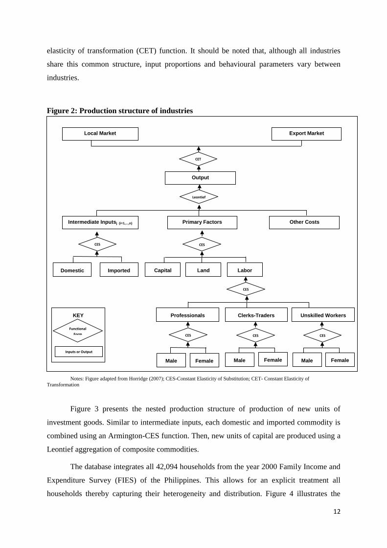
services, including government services (Table ). Figure 2 illustrates the basic production

structure of the model assuming constant returns. Separability assumptions are likewise

imposed to allow producer input and output decisions to be divided into a series of nests. In

this structure, industry output is determined via a four-stage optimization process. The initial

stage involves the optimal determination of male and female labour, using a Constant

Elasticity (CES) function, to form a composite labour for each skill category (professionals,

clerks and trade, and unskilled workers). Then, the skill categories are combined using a CES

function to form a composite of labour input in the second stage. The optimal labour input is

then combined with land and capital to form a CES aggregate of primary factors in the third

stage. At the same time, each domestic and imported commodity is combined using an

Armington-CES function to form an intermediate input composite. Finally, industry output is

determined through a Leontief (linear) determination of primary factor composites,

intermediate input composites and other costs.

As shown in the top-most nest of Figure 2, output for each industry is then allocated

to domestic production between export supply and domestic sales are governed by a constant

0.0

10.0

20.0

30.0

40.0

50.0

60.0

Year

Percent

All 49.2 45.4 45.2 40.6 33.0 34.0 Nat'l Capital Region 27.1 25.1 16.6 10.4 6.5 7.6 Urban 43.9 39.4 42.7 34.7 23.4 23.1 Rural 56.4 52.3 55.0 53.1 46.3 48.8

1985 1988 1991 1994 1997 2000

12

elasticity of transformation (CET) function. It should be noted that, although all industries

share this common structure, input proportions and behavioural parameters vary between

industries.

Figure 2: Production structure of industries

Note: Land input is only used in agriculture

Notes: Figure adapted from Horridge (2007); CES-Constant Elasticity of Substitution; CET- Constant Elasticity of

Transformation

Figure 3 presents the nested production structure of production of new units of

investment goods. Similar to intermediate inputs, each domestic and imported commodity is

combined using an Armington-CES function. Then, new units of capital are produced using a

Leontief aggregation of composite commodities.

The database integrates all 42,094 households from the year 2000 Family Income and

Expenditure Survey (FIES) of the Philippines. This allows for an explicit treatment all

households thereby capturing their heterogeneity and distribution. Figure 4 illustrates the

Output

Intermediate Inputsj (i=1,...,n)

Leontief

CES CES

Domestic Imported Capital

Primary Factors Other Costs

Land Labor

CES

Professionals

CET

KEY

Functional

Form

Inputs or Output

Export Market

Local Market

CES

Female Male

Clerks-Traders

Unskilled Workers

CES CES

Male Male Female Female

13

nesting structure for household demands. It is similar to demand for investment goods, except

that the commodity composites are aggregated by a Linear Expenditure System (LES) utility

function. The LES structure imposes the property that each consumer requires a minimum

level of consumption which is purchased regardless of the price. Any residual is then devoted

for luxury or supernumerary expenditure, which are consequently allocated to each good

based on marginal budget shares.

Figure 3: Demand for investment goods

Note: Land input is only used in agriculture

Notes: Figure adapted from Horridge (2007); CES-Constant Elasticity of Substitution; CET- Constant Elasticity of

Transformation

Figure 4: Household consumption structure

Note: Land input is only used in agriculture

Notes: Figure adapted from Horridge (2007); CES-Constant Elasticity of Substitution; LES- Linear Expenditure System

Export goods are classified into individual export commodity and collective exports—

the former include all main export commodities and are modelled individually, while the

New Capital for Industry i

Good 1

Leontief

CES CES

Domestic Imported

... up to...

KEY

Functional

Form

Inputs or Output

Good C

Domestic Imported

Household consumption/Utility

Good 1

LES

CES CES

Domestic Imported

... up to...

KEY

Functional

Form

Inputs or Output

Good C

Domestic Imported

14

latter include exports which do not mainly to respond on the export price, like service

commodities. Foreign demand for individual export commodity is assumed to be inversely

related to that commodity‘s price. In contrast, the commodity composition of aggregate

collective exports is exogenised by treating collective exports as Leontief aggregate. Demand

for this aggregate is related to its average price via a constant elasticity of demand (CED)

curve, similar to those for individual exports.

Other final demands are modelled differently. Government demand level and

composition of government demand is exogenously determined. In this application, aggregate

government consumption moves with household consumption. Inventories are assumed to

follow domestic production. That is, the percentage change in the volume of each

commodity—domestic or imported—going to inventories, is the same as the percentage

change in the domestic production of that commodity. On the other hand, margin demands

are determined as proportional to the commodity flows with which margins are associated.

In summary, the model behaves under a neo-classical framework. The demand side

assumes cost minimization, whereas the supply side assumes profit maximization. Hence,

both their first-order conditions generate the necessary demand functions (import, export and

domestic) as well as the necessary supply and input demand functions.

5. Simulations and analysis of results

The actual reduction in Philippine export volumes as a result of the economic crisis is

shown in Table 5. We use these values as policy shocks to simulate a reduction in export

demand volume facing the Philippine economy. The shock is applied into the export demand

equation:

𝐗𝟒 𝐜 = 𝐅𝟒𝐐 𝐜 𝐏𝟒 𝐜

𝐏𝐇𝐈 ∗ 𝐅𝟒𝐏 𝐜

𝐄𝐗𝐏𝐄𝐋𝐀𝐒𝐓 𝐜

1

Where: c – Commodity; X4 – Export volume; F4Q – Export quantity shifter; P4 – Price of export;

PHI – Exchange rate; F4P – Export price shifter; EXPELAST – Export elasticity;

From this equation, exports of particular commodities may be fixed or shocked by

making the corresponding elements of the vector x4 exogenous, while at the same time

endogenising matching elements of the vector f4q. To have an idea of the order of magnitude,

results based on a short-run and long-run perspective are likewise analyzed.

15

Table 5: Reduction in exports (% change)

Sector Reduction in exports

Paddy Rice -68.1

Corn -17.51

Coconut -40.59

Fruits and Vegetables -7.02

Raw Sugar and Sugar cane 19.99

Other Crops -26.23

Livestock -17.51

Poultry -17.51

Fishing and Forestry -12.99

Other Agriculture -17.51

Mining -41.2

Processed Meat and Fish -11.44

Other Processed food -11.44

Rice and Corn Milling -68.1

Sugar Milling 30

Tobacco and Alcohol 54.59

Textiles -23.255

Garments and Footwear -28.73

Paper and Wood products -10.66

Chemicals -14.64

Petroleum -76.62

Cement and Metal -25.93

Machineries -10.87

Electric related and Appliances -22.2

Semi-conductors -26

Transport Machineries -10.87

Other Manufacturing -9.35 Source: National Statistical Office (2010)