global equity momentum - investresolve.com · global equity momentum - a raftsman’s erspective 7...

GLOBAL EQUITY MOMENTUMA CRAFTSMAN'S PERSPECTIVE

Global Equity Momentum - A Craftsman’s Perspective

2 ReSolve Asset Management

Global Equity Momentum – A Craftsman’s Perspective 3

Key Takeaways 3

Global Equity Momentum 5

Defining Trend and Momentum 6

Specification Risk 8

Setting Expectations 9

Same Same - But Different 12

In Sample vs. Out of Sample 16

The Ensemble Approach 18

Validating Ensemble on Simulated Data 28

Tax Discussion 34

Craftsmanship Tax Alpha 36

Conclusion 38

TABLE OF CONTENTS



KEY TAKEAWAYS

• Quantitative investment researchers often focus their efforts on identifying the best single parameterization of their strategy, but this ignores a critically important feature of investing. Specifically, focusing on parameter choices independently overlooks the potential opportunity for diversification across the same approach specified with different parameter choices.

• We examine this concept under the microscope using Dual Momentum - and in particular Global Equity Momentum - as our case study.

• We are concerned with the extent to which changes in lookback horizons for momentum or trend have impacted the historical results of Global Equity Momentum strategies over both shorter and longer investment horizons. We find that the Global Equity Momentum approach is robust to a surprisingly wide range of specifications. In fact, we perform a variety of robust statistical tests and find that we cannot reject the view that all of our strategy specifications have equal merit.

• In view of our conclusion that a wide variety of Global Equity Momentum specifications have equal merit, we investigate the potential to combine many different specifications in an “ensemble” strategy. The idea is to focus on the underlying styles that are providing an edge - trend and momentum - while acknowledging that there are many equally valid ways of specifying and combining these signals.

• We construct many Global Equity Momentum strategies representing combinations of different lookbacks for absolute and relative momentum. Models specified on shorter-term lookbacks for trend and/or momentum will often hold different markets than models specified on intermediate or longer-term lookback horizons, which offers the chance for diversification.

• We also acknowledge that trend and momentum can be measured in a variety of ways, and introduce a slight variation based on moving averages. To the extent that the signals produced from any one specification are out of sync with markets in any period, we can reduce the dispersion in performance by using signals from multiple specifications.

• We find that an ensemble strategy that combines the target weights from all of our alternative specifications in each period produced attractive long-term returns that effectively captured the Global Equity Momentum style premia.

• However, the ensemble produced its performance with lower volatility and smaller drawdowns. Perhaps the most important take-away from our analysis is that the ensemble methods produced much more stable performance over shorter investment horizons on the order of five or ten years, which matter most to investors.

GLOBAL EQUITY MOMENTUM - A CRAFTSMAN’S PERSPECTIVE



• We examine the tax impact of an ensemble approach relative to a single specification that emphasizes longer-term trend and momentum signals. The ensemble produces many more trades and accrues approximately 0.5% per year in excess taxes.

• We analyze how much turnover we might expect from noise trading and implement a trade filter that profoundly reduces turnover for the ensemble approach and almost completely eliminates the excess tax burden. The ensemble method preserves all of its extensive performance benefits on an after-tax basis.

GLOBAL EQUITY MOMENTUM

The 2012 paper “Risk Premia Harvesting through Dual Momentum” proposed a simple method combining three premier anomalies – the equity risk premium along with trend and momentum – to produce stronger returns with gentler drawdowns. Gary’s paper followed work by others like Cliff Asness, Meb Faber, Wang and Kochard, Blitz and van Vliet, and an even larger body of evidence from the managed futures space, documenting strong effects from trend and momentum.

The author, Gary Antonacci, later published an excellent book on “Dual Momentum” that covered the concepts from many different angles. In his book and on his blog, Gary has examined a variety of strategies that harnessed the Dual Momentum concept. Over time, perhaps due to the strong performance of stocks relative to other asset classes since 2012, Gary’s Global Equity Momentum strategy has grown quite popular. We have regular chats with Advisors and investors who have tried to implement the Global Equity Momentum strategy in one form or another.

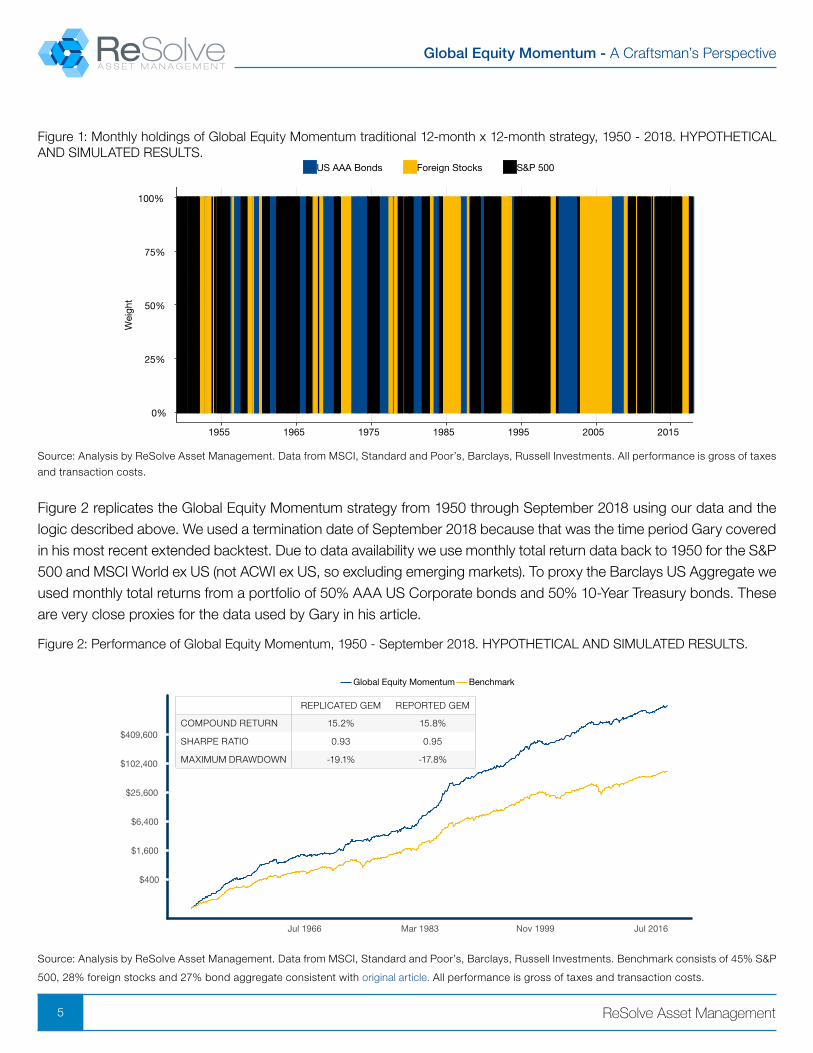
The Global Equity Momentum strategy observes the total returns to broad U.S. equities (S&P 500) and foreign equities (ACWI ex-US) on a monthly basis over a rolling lookback window of 12-months. If the S&P 500 had positive returns over the past 12-months (positive trend) the strategy allocates to stocks the next month; otherwise it allocates to bonds (Barclays US Aggregate). When the trend is positive for stocks the strategy holds the equity index with the strongest total return over the same horizon. Figure 1 shows the evolution of portfolio holdings for Gary’s original 12-month x 12-month implementation since 1950.

https://papers.ssrn.com/sol3/papers.cfm?abstract_id=2042750



http://www.dualmomentum.net/

https://www.dualmomentum.net/2018/10/extended-backtest-of-global-equities.html



Figure 1: Monthly holdings of Global Equity Momentum traditional 12-month x 12-month strategy, 1950 - 2018. HYPOTHETICAL AND SIMULATED RESULTS.

0%

25%

50%

75%

100%

1955 1965 1975 1985 1995 2005 2015

Wei

ght

US AAA Bonds Foreign Stocks S&P 500

Source: Analysis by ReSolve Asset Management. Data from MSCI, Standard and Poor’s, Barclays, Russell Investments. All performance is gross of taxes

and transaction costs.

Figure 2 replicates the Global Equity Momentum strategy from 1950 through September 2018 using our data and the logic described above. We used a termination date of September 2018 because that was the time period Gary covered in his most recent extended backtest. Due to data availability we use monthly total return data back to 1950 for the S&P 500 and MSCI World ex US (not ACWI ex US, so excluding emerging markets). To proxy the Barclays US Aggregate we used monthly total returns from a portfolio of 50% AAA US Corporate bonds and 50% 10-Year Treasury bonds. These are very close proxies for the data used by Gary in his article.

Figure 2: Performance of Global Equity Momentum, 1950 - September 2018. HYPOTHETICAL AND SIMULATED RESULTS.

$400

$1,600

$6,400

$25,600

$102,400

$409,600

Jul 1966 Mar 1983 Nov 1999 Jul 2016

Global Equity Momentum Benchmark

Source: Analysis by ReSolve Asset Management. Data from MSCI, Standard and Poor’s, Barclays, Russell Investments. Benchmark consists of 45% S&P

500, 28% foreign stocks and 27% bond aggregate consistent with original article. All performance is gross of taxes and transaction costs.

REPLICATED GEM REPORTED GEM

COMPOUND RETURN 15.2% 15.8%

SHARPE RATIO 0.93 0.95

MAXIMUM DRAWDOWN -19.1% -17.8%




Our results track Gary’s results very closely. We are confident that the small deltas observed in our results are due to minor differences in the underlying indices used for our analysis. You will see below that small changes to underlying indexes can have surprisingly large effects on long-term results.

For the balance of this article we will refer to this specification of Global Equity Momentum - with 12-month lookbacks for both absolute and relative momentum - as the “Original” specification. Also note that we may use the terms “absolute momentum”, “trend”, or “time-series momentum” interchangeably. We may also substitute “cross-sectional momentum” or “relative strength” for the term “relative momentum”.

DEFINING TREND AND MOMENTUM

SECTION TAKEAWAYS

• The edges harvested by Global Equity Momentum - trend and momentum effects - are omnipresent across time, geographies, and asset classes with several compelling explanations.

• Different specifications of Global Equity Momentum in terms of lookback horizon and/or measure of trend can produce large dispersion in short-term returns

• Over the 10-year period from 2009 through 2018 a Global Equity Momentum strategy formed on 10-month returns outperformed the same strategy formed on 9-month returns by over 100 percentage points.

• The choice of a single model specification – in the case of GEM the lookbacks chosen for the measurement of relative and absolute momentum – may be a large and uncompensated source of risk.

Global Equity Momentum is designed to take advantage of momentum and trend effects, which have been documented in virtually every market and over centuries of data. These are omnipresent and extremely economically significant phenomena. Our goal should be to extract the maximum amount of “signal” from these noisy processes while minimizing the potential for bad luck along the way.

It’s important when designing an investment strategy to start with first principles: why is there a persistent effect that offers an opportunity for profit, and how might these potential explanations inform how we should specify our model? Momentum and trend are close cousins, and have similar explanations related to herding, benchmarking and information diffusion. Investors experience a fear of missing out (or “FOMO”) and/or overreact to near-term good or bad news. And it takes time for different classes of investors to learn about and gain confidence to act upon a potential shift in underlying fundamentals.

The process of FOMO or the time period of over/underreaction and information diffusion are not deterministic. There is no time-frame or magnitude of shift in prices or fundamentals that always invokes momentum or trend behaviour. Rather, across markets and time periods we see that momentum and trend effects seem to manifest over periods



spanning a few months to a year or more. And since it is equally likely to observe trend and momentum behaviour at any of these horizons, there are no obvious reasons to choose any particular one.

Recently there have been some insightful articles by luminaries like Corey Hoffstein and Gary himself about the optimal specification for a Global Equity Momentum approach. Corey showed that Global Equity Momentum strategies with formation periods between 6 and 12-months produced wildly disperse results over the past ten calendar years. Over the ten years from 2009 - 2018 a Global Equity Momentum strategy formed on a 10-month lookback produced a total return of 146% while the same strategy formed on a 9-month lookback grew just 43%. Moreover, in 2010 a GEM model with a 9-month lookback lost 9.31% while a model specified with a 10-month lookback gained 12.21% for a 21% percentage point difference in return in a single calendar year.

Corey’s illustration hinted at why the choice of a single model specification – in the case of GEM the lookbacks chosen for the measurement of relative and absolute momentum – may be a large and uncompensated source of risk. Investors have the opportunity to diversify away this risk to produce similar expected returns with lower risk by running many similar models that harness the same underlying inefficiency or risk, but that view the “signals” from a slightly different perspective.

SPECIFICATION RISK

SECTION TAKEAWAYS

• None of the explanations for trend or momentum prescribe any particular definition for how to define “trend” or “momentum” or specify optimal theoretical lookbacks to harvest these effects.

• We test Global Equity Momentum strategies across 18 possible parameterizations of trend lookbacks and 18 possible parameterizations of momentum lookbacks for a total of 324 strategy combinations.

• We also test trend and momentum strategies defined using prices relative to moving averages.

• We use two methods to signal when to move from stocks into bonds: the original method using just the trend of the S&P 500, and a method that requires that both U.S. and foreign stocks are in negative trends.

The Original Global Equity Momentum specification used a portfolio formation period (i.e. lookback period) of 12-months for both absolute (i.e. time-series) and relative (i.e. cross-sectional) measures of momentum. Gary’s article cites several examples of prior literature supporting these choices. We support the conclusion that a 12-month lookback period is reasonable and likely to produce good long-term performance.

While the Original specification is perfectly valid and consistent with prior literature, we are not aware of any fundamental or deterministic reasons why a 12-month lookback horizon should produce optimal results. A review of literature on time-series and cross-sectional momentum, including some of the articles cited above, suggests that lookback horizons from

https://blog.thinknewfound.com/2019/01/fragility-case-study-dual-momentum-gem/

https://www.dualmomentum.net/



1-month through 12-months, and perhaps even longer formation periods, have produced good long-term performance. Standard tests imply that a surprisingly wide range of specifications are equally legitimate from a statistical perspective.

We tested this thesis by constructing Global Equity Momentum strategies representing all possible combinations of absolute and relative momentum formed on 1-18 month lookbacks. With 18 possible parameterizations of trend lookbacks and 18 possible parameterizations of momentum lookbacks, there are 324 possible strategy combinations.

We also recognize that there are equally valid alternative definitions of “absolute” and “relative” momentum that capture the same effects, but from a slightly different perspective1. Investors have defined “trend” in many ways over the years including moving average cross (price minus moving average), dual moving average cross, triple moving average cross, Donchian, MACD, Bollinger breakout, etc. One could also define trends based on risk-adjusted measures like Sharpe, Sortino or Omega ratios, or using methods like “Point and Figure” models.

For simplicity, we added a moving average cross strategy to our investigation alongside the original time-series approach. Specifically, we measured momentum as the percentage difference between the current price of the market and a moving average. All other logic is consistent with the Global Equity Momentum rules. Since we are using monthly data we are limited to using moving average strategies with lookbacks from 2 through 18 months. There are 289 ways to combine 2-18 month absolute momentum lookbacks with 2-18 relative momentum lookbacks.

Note that Gary’s specification moves into bonds only when the S&P 500 closes out a month with a negative trend. This is an important detail that may have a meaningful impact on long-term results. Gary reasoned that the S&P 500 should provide the most robust trend signal because it is the most liquid and diversified market. It also derives meaningful revenue from foreign markets, so it is sensitive to global economic momentum.

These are reasonable arguments, but we were curious whether we might derive a more nuanced and balanced signal by making use of trend information from both indexes. Specifically, we investigated strategies that moved into bonds only if the S&P 500 AND foreign stocks BOTH exhibited negative trends.

To summarize, we ran the following strategy combinations:

Traditional Global Equity Momentum strategy based total returns versus cash over lookbacks from 1 to 18 months, and where the move into bonds is conditioned on: * S&P 500 in negative trend (324 specifications) * S&P 500 AND foreign stocks in negative trend (324 specifications)

Moving Average Global Equity Momentum strategy based on the percentage difference between the current price and a moving average versus cash over lookbacks from 2 to 18 months, and where the move into bonds is conditioned on: * S&P 500 in negative trend (289 specifications) * S&P 500 AND foreign stocks in negative trend (289 specifications).

1 For more on this see https://investresolve.com/blog/dynamic-asset-allocation-for-practitioners-part-2-the-many-faces-of-price-momentum/

http://stockcharts.com/school/doku.php?id=chart_school:chart_analysis:pnf_charts:pnf_basics

https://investresolve.com/blog/dynamic-asset-allocation-for-practitioners-part-2-the-many-faces-of-price-momentum/



Each of the traditional time-series approaches spawn 324 specifications and each moving average approach spawns 289 specifications for a total of 1226 total sub-strategy specifications.

SETTING EXPECTATIONS

SECTION TAKEAWAYS

• Prior literature on trend and momentum find significant effects across a range of lookback horizons, though academically oriented papers have tended to focus on the precedent of a 12-month horizon.

• A seminal paper on trend-following showed that 1-, 3- and 12-month lookbacks yielded strong and statistically indistinguishable results over 137 years when applied to a diversified futures universe. This implies that they are all harvesting a similar effect with similar effectiveness, but from slightly different perspectives.

• A combination or “ensemble” of strategies produced a substantial boost in risk-adjusted performance.

• Perhaps the most unbiased estimate of future performance for any strategy specification is the median performance across all strategies tested. We hypothesize that the expected performance of an ensemble of equally legitimate strategies will dominate the performance of any individual strategy specification.

The development of trading strategies requires analysts to fit rules to historical market data in order to produce profits in live trading. Obviously, different rules applied to different markets will produce different results so the research process involves finding combinations of rules and markets that have produced favorable outcomes in prior periods.

In many cases the investigation of trading strategies is inspired by research published by academics or other practitioners. Our earliest adventures in quantitative research were inspired by people like Meb Faber, Cliff Asness and Gary Antonacci himself. Meb cites inspiration from Jeremy Siegel, who examined a 200-day moving average strategy applied to U.S. stocks in his book, “Stocks for the Long Run”. Jeremy describes how he was inspired by Martin Zweig, who was inspired by William Gordon, who described a method proposed by H.M. Gartley in a book 2 that was first published in 1930!

In specifying the parameters for his Global Equity Momentum strategy Gary primarily cites Jegadeesh and Titman and Moskowitz, Ooi and Pedersen to justify his choice of a 12-month lookback for both absolute and relative momentum signals. Jegadeesh and Titman explored the performance of relative strength strategies on stocks over horizons from three to twelve months, skipping the first month. They found statistically significant effects for long-short strategies formed on all lookbacks studied, though the effects were strongest at 12-months. Notably, the performance of the long “legs” of the portfolios produced equally strong statistical significance (t-stats ~4) across all lookback horizons. In other words, long-only momentum investors should be equally motivated to invest in strategies that form portfolios on a 3-month, 6-month, 9-month or 12-month lookback horizons.

2 Profits in the Stock Market,New York: H.M. Gartley, 1930.

http://www.business.unr.edu/faculty/liuc/files/BADM742/Jegadeesh_Titman_1993.pdf




Moskowitz, Ooi and Pedersen’s paper examined the “time-series momentum” factor specified with a 12-month lookback horizon on a diversified basket of futures contracts. This paper was academic in focus, as evidenced by the fact that it was published in the prestigious Journal of Financial Economics. Thus, the authors followed the academic practice of focus on a single factor specification to examine the economic motivations for the factor premium. However, they also analyzed alternative specifications with different lookback horizons and found them all to be statistically and economically significant.

Moskowitz’ co-authors Ooi and Pedersen also published a practitioner oriented paper called A Century of Evidence on Trend Following with Brian Hurst that was published in the Fall 2017 edition of the Journal of Portfolio Management. This paper examined diversfied trend strategies specified with 1-, 3- and 12-month lookback horizons back to 1880. We present Exhibit 2 from the paper in Figure 3 and highlight the full-sample Sharpe ratios produced by each lookback specification. Note that all lookbacks produced similar gross long-term risk-adjusted performance over the 137-year sample.

Figure 3: Exhibit 2 from Hurst, Ooi and Pedersen “A Century of Trend-Following Investing”, 2017. HYPOTHETICAL AND SIMULATED RESULTS.

Performance of Time-Series Momentum by Signal

Time Period1-Month Strategy

1-Month Strategy (lagged)

3-Month Strategy


12-Month Strategy


Full Sample Jan 1880 - Dec 2016

1.38 0.45 1.19 0.64 1.32 1.04

By Decade

Jan 1880-Dec 1889 1.02 -0.34 0.78 -0.23 1.03 0.89

Jan 1890-Dec 1899 1.32 0.34 0.91 0.25 1.35 0.83

Jan 1900-Dec 1909 0.87 0.35 1.20 0.65 1.52 1.52

Jan 1910-Dec 1919 0.80 0.01 0.63 0.39 0.99 0.83

Jan 1920-Dec 1929 1.75 0.56 1.23 0.51 1.77 1.27

Jan 1930-Dec 1939 1.19 0.27 1.21 0.29 1.09 0.70

Jan 1940-Dec 1949 2.16 1.09 1.65 1.29 1.54 1.27

Jan 1950-Dec 1959 2.48 1.48 1.95 1.38 1.55 1.27

Jan 1960-Dec 1969 1.81 0.31 1.31 0.68 1.01 0.42

Jan 1970-Dec 1979 2.24 0.82 2.13 1.34 1.91 1.66

Jan 1980-Dec 1989 1.77 0.40 1.09 0.50 1.46 1.07

Jan 1990-Dec 1999 1.13 0.49 1.52 0.75 1.38 1.20

Jan 2000-Dec 2009 0.70 0.38 0.67 0.66 1.10 0.86

Jan 2010-Dec 2016 0.06 0.13 0.30 0.33 0.73 0.70

Source: Hurst, Ooi and Pedersen A Century of Evidence on Trend Following, JPM Fall 2017. All performance is gross of taxes and transaction costs.

Figure 3 offers an interesting case for a discussion of expected performance. Trend strategies formed on 1-month, 3-months and 12-months all produced similar risk-adjusted performance over 137 years. For the moment let’s caveat some important details like transaction costs and taxes. We’ll get to those topics in a moment (and offer some potentially

https://www.aqr.com/-/media/files/papers/aqr-jpm-fall-2017.pdf





surprising elucidations). In the context of the information that we have, which strategy is most likely to produce the best performance going forward? And what performance should we expect?

The 12-month lookback specification proved much more resilient to lagged trading. But should this be surprising? A 1-month delay in trading on a 1-month lookback means that 1-month / 1-month = 100% of the information that was used to generate the signal is stale when the signal is traded. A 1-month delay in trading on a 3-month signal means that 1-month / 3-months = 33% of the information is stale, while a 1-month delay on a 12-month signal means that just 1-month / 12-months = 8.3% of the information is stale. The lagged results reflect this exact phenomenon as the 1-month strategy shows much larger decay than the 3-month strategy, and the 12-month strategy shows almost no impact from lagged trading.

Lacking other data, some investors might choose the slower-moving 12-month lookback specification because it will probably require less trading activity. It may also produce less turnover and taxes, though we should not take this for granted. Several papers see for example have shown that trend following strategies tend to crystallize a large number of small losses against a small number of very large gains, which makes them relatively tax efficient. The losses tend to be short-term while the gains tend to be longer-term. We perform a more direct investigation of tax implications below.What performance should we expect from the 12-month trend strategy? It produced a Sharpe ratio of 1.32 in-sample. Is that our best estimate? We contend that the other two strategies are harnessing the same effect, and, as we will show below, have equal merit. Shouldn’t we use information from those strategies to help inform our expectations for the 12-month strategy?

We submit that since all three specifications produced statistically indistinguishable Sharpe ratios, the performance difference between the strategies over any given period is a result of random noise. If this is true, the expected performance for any single trend strategy specification is the median performance observed across all strategy specifications. The median Sharpe ratio across the three trend specifications is also 1.32 (since the Sharpe ratio of the 12-month strategy lies between the 1-month and 3-month Sharpe ratios).

But this prompts an important question: if all of the specifications have equal merit, but they produce strong and/or weak performance at different times, why not allocate to all three strategies at once? It turns out that the Sharpe ratio of an equally weighted combination of the 1-, 3- and 12-month diversified trend strategies produced a gross Sharpe ratio of 1.86 3. The equal-weight combination strategy produced performance well beyond the average performance of the individual strategies because the individual strategies are relatively uncorrelated and provide diversification of signals.We expect a similar phenomenon to emerge from our investigation of Global Equity Momentum. The Original specification used a 12-month lookback for both trend and momentum and moved from stocks to bonds excusively on the basis of the S&P 500 trend signal. However, our base case is that there is nothing magical about this particular approach. Rather, we hypothesize that all of the Global Equity Momentum specifications that we described above have equal theoretical merit, so momentum and trend effects should be statistically indistinguishable across a wide variety of lookbacks. Similarly, we also expect to find that it is equally legitimate to define trend versus a moving average, and to

3 Exhibit 1 of the Hurst, Ooi and Pedersen paper shows gross excess returns were 18% on volatility of 9.7% for an equal weight mix of strategies formed on the three lookback horizons.

http://www.cis.upenn.edu/~mkearns/finread/trend.pdf



use both S&P 500 and foreign stocks to inform our trend signals.

In summary, we expect that since all of our specifictions are attempting to harness the exact same style premia - trend and momentum - we should expect them to generate precisely the same edge ex ante. Therefore, a reasonable estimate for the future performance of any of our model specifications should be the median performance across all specifications, and given a long enough investment period the performance of all of our specifications will converge on the median.

SAME SAME - BUT DIFFERENT

SECTION TAKEAWAYS

• We test the null hypothesis that there is no statistical difference between the performance of the Original Global Equity Momentum strategy and the other alternative specifications.

• We observe that there is almost no difference between many return samples drawn from the distribution of Original strategy returns and the many return samples drawn from alternative strategy returns, on average.

• We conclude that the Original strategy has the same population compound mean as all of our other strategy specifications within reasonable statistical bounds.

• A reasonable estimate of future performance for any strategy specification is the median performance across all of our strategy specifications.

Our next step is to determine if there is a statistical difference between the Original Global Equity Momentum specification and our 1225 alternative specifications. We will examine the distribution of compound returns, but we could perform similar tests on other performance statistics like Sharpe ratio, drawdowns, or virtually any other measure.

We performed block bootstrap tests on the differences in compound returns between Gary’s original model and all 1225 alternative models. Bootstrapping is a form of Monte Carlo analysis where monthly returns are drawn randomly from the distribution of actual realized returns. Each time a return is drawn it is placed back in the distribution so that it can be drawn again. The advantage of bootstrap over parametric Monte Carlo analysis is that it preserves the empirical shape of the return distribution rather than assuming returns conform to traditional shapes like Gaussian or Poisson distributions.

Traditional bootstraps draw returns randomly so that the next draw is completely independent of the previous draw. This approach will eliminate any relationships that might exist between adjacent monthly returns such as autocorrelation effects. Block bootstrapping involves drawing “blocks” of contiguous observations in order preserve to the greatest degree possible any conditional return dynamics (e.g. auto-correlation of time-series returns, heteroskedastic volatility,



etc.) that existed in the original data. Random blocks of observations are chosen where each block contains a random number of observations. The average number of observations per block is chosen in order to minimize the mean squared error between the bootstrap variance and the variance of the original sample 4.

For each of our 1225 strategy specifications we created 15,000 block bootstrap samples of strategy returns (with replacement) of the same length as the original sample (all 828 months from 1950 - 2018). Each of these samples represents one possible way that the past could have unfolded for this particular strategy specification given all of the monthly returns that we observed in our backtest of that strategy 5. Some of these samples will represent an extremely unlucky experience by drawing a disproportionate share of months with below-average strategy returns, while others will simulate an extremely lucky outcome by drawing a disproportionate share of above-average returns. Most draws will be somewhere in between. But each of our samples will represent a perfectly legitimate way that an investor might experience the returns from the strategy while preserving the same character as the original backtest of that specification.

We followed the same procedure to simulate 15,000 boostrap samples of returns drawn from Gary’s original strategy.Next we calculated the annualized returns for each bootstrap sample from the alternative specification and for each bootstrap sample from the Original specification. Finally, we subtracted the 15,000 annualized returns sampled from the alternative specification from the 15,000 annualized returns sampled from Gary’s specification. The outcome of this process was a distribution of 15,000 differences in compound annual returns between Gary’s original specification and the alternative specification.

Our null hypothesis is that the compound annual returns from the Original strategy have the same mean as the compound annual returns from our alternative strategy. If this is true, the average of the 15,000 differences in means produced from our bootstrap analysis should be statistically indistinguishable from 0. In other words, on average we should observe that there is almost no difference between the many returns drawn from the Original strategy and the many returns drawn from the alternative strategy.

4 See [ ftp://ftp.stat.math.ethz.ch/Research-Reports/52a.ps.gz ] for details on on this approach.

5 To be clear, we bootstrapped the strategy returns themselves, not the individual market returns.

ftp://ftp.stat.math.ethz.ch/Research-Reports/52a.ps.gz



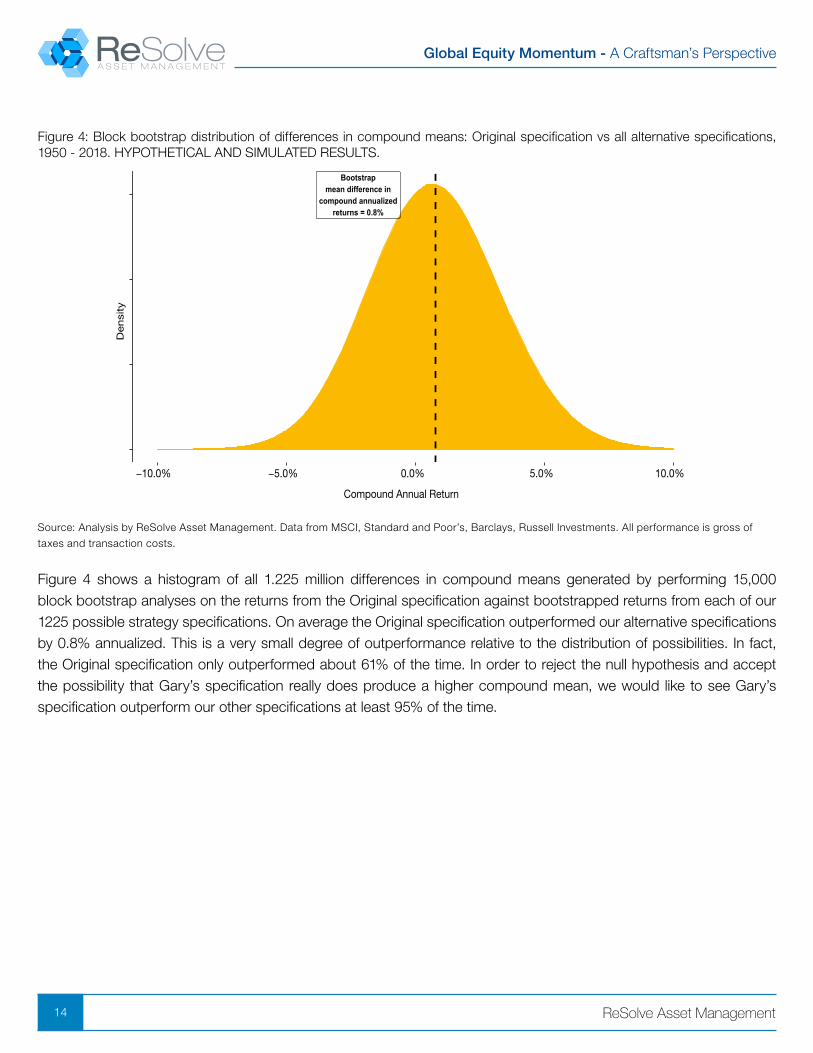
Figure 4: Block bootstrap distribution of differences in compound means: Original specification vs all alternative specifications, 1950 - 2018. HYPOTHETICAL AND SIMULATED RESULTS.

Bootstrapmean difference in

compound annualizedreturns = 0.8%

−10.0% −5.0% 0.0% 5.0% 10.0%

Compound Annual Return

Densi

ty

Source: Analysis by ReSolve Asset Management. Data from MSCI, Standard and Poor’s, Barclays, Russell Investments. All performance is gross of

taxes and transaction costs.

Figure 4 shows a histogram of all 1.225 million differences in compound means generated by performing 15,000 block bootstrap analyses on the returns from the Original specification against bootstrapped returns from each of our 1225 possible strategy specifications. On average the Original specification outperformed our alternative specifications by 0.8% annualized. This is a very small degree of outperformance relative to the distribution of possibilities. In fact, the Original specification only outperformed about 61% of the time. In order to reject the null hypothesis and accept the possibility that Gary’s specification really does produce a higher compound mean, we would like to see Gary’s specification outperform our other specifications at least 95% of the time.



Figure 5: Proportion of block bootstrap samples where compound mean of Original specification exceeds compound mean of alternative specification, 1950-2018. HYPOTHETICAL AND SIMULATED RESULTS.

0%

25%

50%

75%

100%

Sub−Strategy

Perc

enta

ge o

f b

lock b

oo

tstr

ap

s w

here

annualiz

ed

retu

rns

of

Orig

inal s

peci�

catio

n a

re g

reate

r th

an t

he a

nnualiz

ed

retu

rno

f th

e a

ltern

ative

sp

eci�

catio

n.



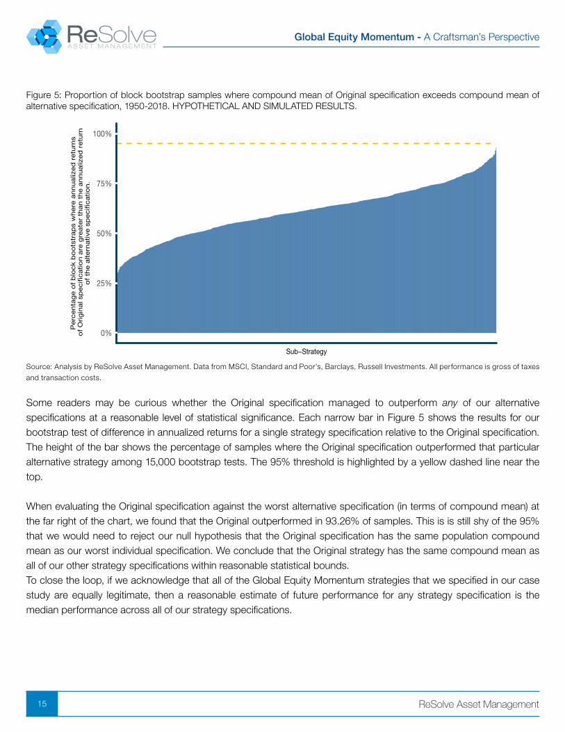
Some readers may be curious whether the Original specification managed to outperform any of our alternative specifications at a reasonable level of statistical significance. Each narrow bar in Figure 5 shows the results for our bootstrap test of difference in annualized returns for a single strategy specification relative to the Original specification. The height of the bar shows the percentage of samples where the Original specification outperformed that particular alternative strategy among 15,000 bootstrap tests. The 95% threshold is highlighted by a yellow dashed line near the top.

When evaluating the Original specification against the worst alternative specification (in terms of compound mean) at the far right of the chart, we found that the Original outperformed in 93.26% of samples. This is is still shy of the 95% that we would need to reject our null hypothesis that the Original specification has the same population compound mean as our worst individual specification. We conclude that the Original strategy has the same compound mean as all of our other strategy specifications within reasonable statistical bounds.To close the loop, if we acknowledge that all of the Global Equity Momentum strategies that we specified in our case study are equally legitimate, then a reasonable estimate of future performance for any strategy specification is the median performance across all of our strategy specifications.



IN SAMPLE VS. OUT OF SAMPLE

SECTION TAKEAWAYS

• Previous analysis showed that we can’t reject the conclusion that the Original specification has the same population mean as our other strategy specifications.

• A reasonable estimate for performance of the Original strategy out-of-sample is the median performance across all strategy specifications.

• The period 1950-1973 and 2012-2018 are true out-of-sample periods since the original paper was published in 2012 and tested on data from 1974-2011.

• While the Original strategy outperformed in-sample, we show that its performance converges to the median in the out-of-sample period.

• This is further validation that the Original specification has the same expected performance as any other strategy specification, and that we should expect the performance of any individual strategy to converge toward the median in the long-term.

Fortunately, the evolution of Gary’s own thinking, and the discovery of new longer-term data sources, offer a perfect opportunity to put the assertions above to the test. Gary first published his paper on Global Equity Momentum in April 2012. In this paper he tested the Global Equity Momentum concept on data from 1974 through 2011.

In a follow-up article called Extended Backtest of Global Equities Momentum Gary extended his backtest into the past using data back to 1950, and extended into the future using data from 2012 - 2018. The sample from 1950-1973 and from 2012-2018 are truly out of sample.

Remember, we have made the case that Gary’s 12x12 specification of Global Equity Momentum has exactly the same expected performance as any of our alternative specifications. Thus, our best estimate for the out of sample performance of Gary’s specification is the median of all alternative specifications.




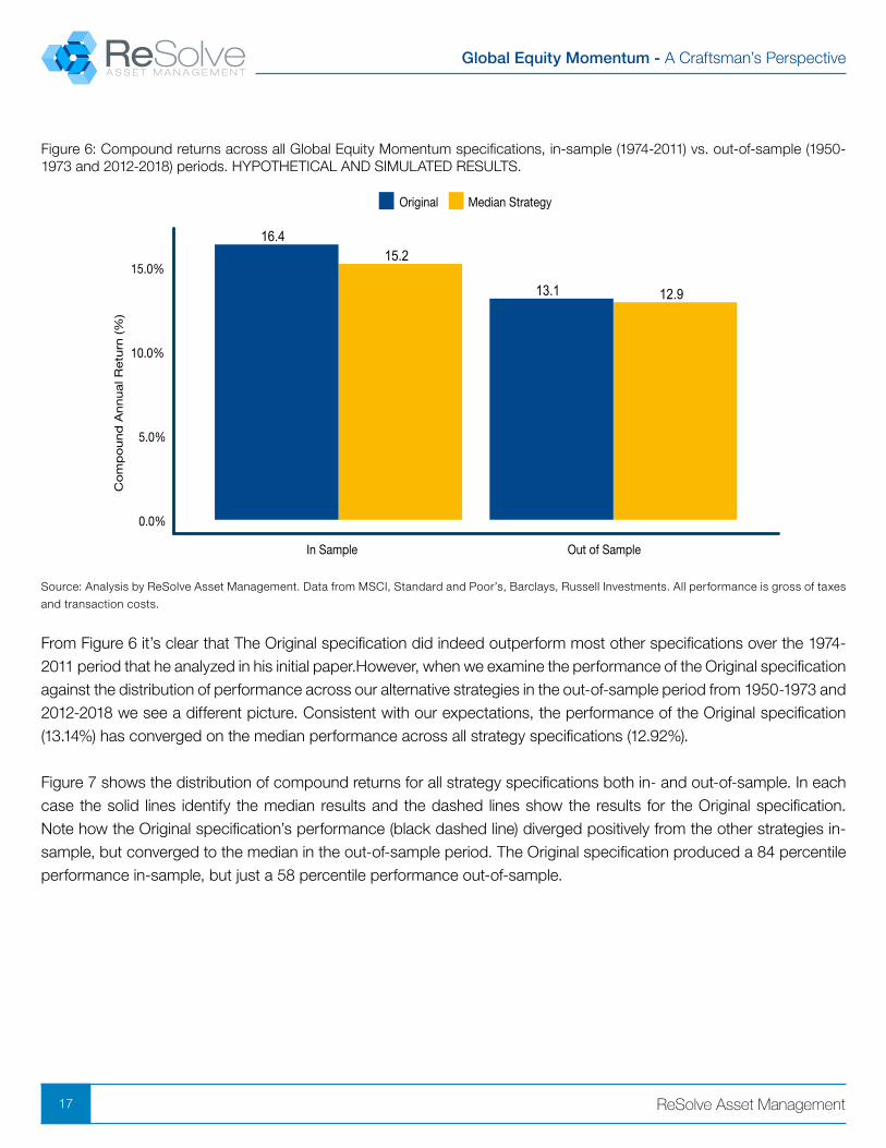
Figure 6: Compound returns across all Global Equity Momentum specifications, in-sample (1974-2011) vs. out-of-sample (1950-1973 and 2012-2018) periods. HYPOTHETICAL AND SIMULATED RESULTS.

15.216.4

12.913.1

0.0%

5.0%

10.0%

15.0%

In Sample Out of Sample

Co

mp

ou

nd

An

nu

al R

etu

rn (%

)

Original Median Strategy



From Figure 6 it’s clear that The Original specification did indeed outperform most other specifications over the 1974-2011 period that he analyzed in his initial paper.However, when we examine the performance of the Original specification against the distribution of performance across our alternative strategies in the out-of-sample period from 1950-1973 and 2012-2018 we see a different picture. Consistent with our expectations, the performance of the Original specification (13.14%) has converged on the median performance across all strategy specifications (12.92%).

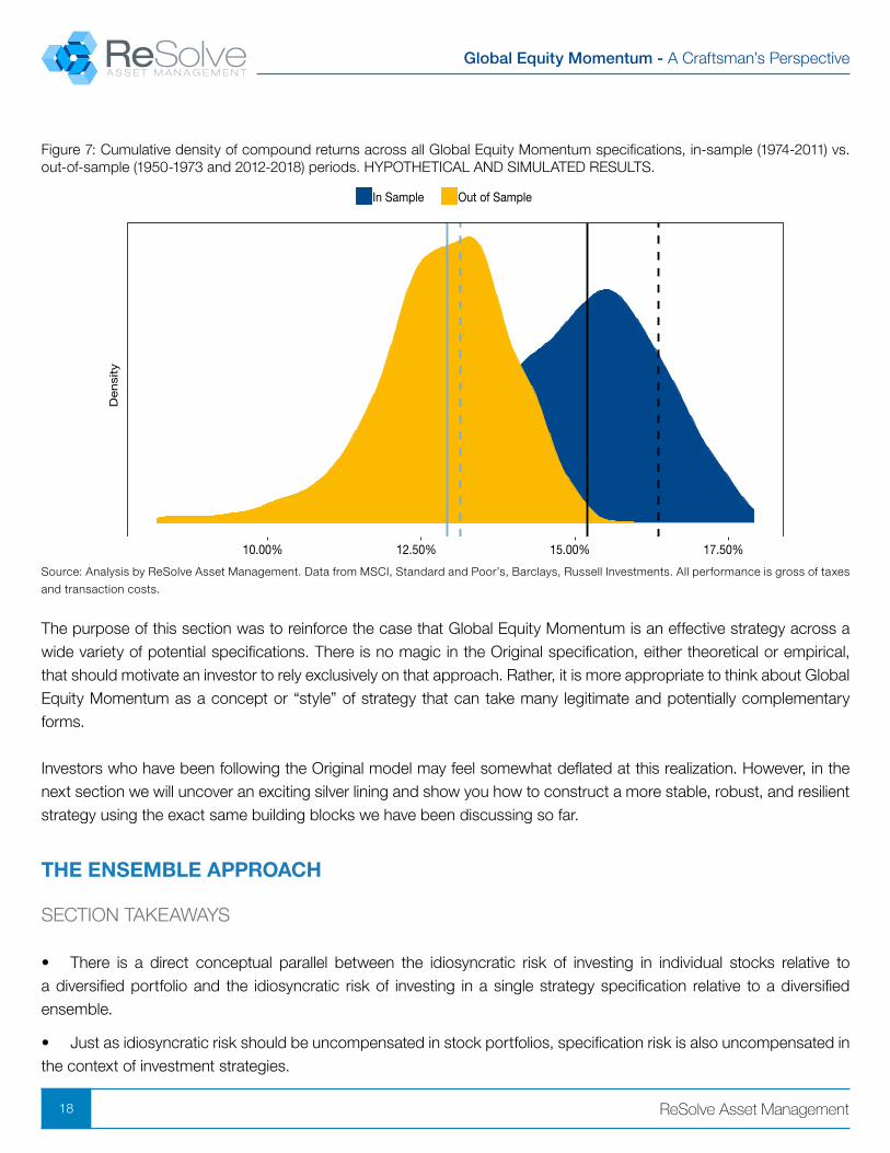
Figure 7 shows the distribution of compound returns for all strategy specifications both in- and out-of-sample. In each case the solid lines identify the median results and the dashed lines show the results for the Original specification. Note how the Original specification’s performance (black dashed line) diverged positively from the other strategies in-sample, but converged to the median in the out-of-sample period. The Original specification produced a 84 percentile performance in-sample, but just a 58 percentile performance out-of-sample.



Figure 7: Cumulative density of compound returns across all Global Equity Momentum specifications, in-sample (1974-2011) vs. out-of-sample (1950-1973 and 2012-2018) periods. HYPOTHETICAL AND SIMULATED RESULTS.

10.00% 12.50% 15.00% 17.50%

Densi

ty

In Sample Out of Sample



The purpose of this section was to reinforce the case that Global Equity Momentum is an effective strategy across a wide variety of potential specifications. There is no magic in the Original specification, either theoretical or empirical, that should motivate an investor to rely exclusively on that approach. Rather, it is more appropriate to think about Global Equity Momentum as a concept or “style” of strategy that can take many legitimate and potentially complementary forms.

Investors who have been following the Original model may feel somewhat deflated at this realization. However, in the next section we will uncover an exciting silver lining and show you how to construct a more stable, robust, and resilient strategy using the exact same building blocks we have been discussing so far.

THE ENSEMBLE APPROACH

SECTION TAKEAWAYS

• There is a direct conceptual parallel between the idiosyncratic risk of investing in individual stocks relative to a diversified portfolio and the idiosyncratic risk of investing in a single strategy specification relative to a diversified ensemble.

• Just as idiosyncratic risk should be uncompensated in stock portfolios, specification risk is also uncompensated in the context of investment strategies.



• Ensemble methods have proved extremely valuable in machine learning competitions and many winners have made abundant use of this technique.

• The ensemble strategy should produce approximately the same return over the long term as any single strategy specification. However, the ensemble investor will usually be subject to less dispersion in results along the way.

• There is a 5% chance that any particular specification might underperform a different specification of Global Equity Momentum by as much as 64 percentage points over five years.

• The ensemble may be expected to produce a slightly higher compound return with a small reduction in volatility. More critically, the ensemble may be expected to deliver much more stable returns.

• This means that investors with finite investment horizons will probably come closer to realizing their target return, with a much smaller risk of adverse outcomes.

• From a financial perspective this translates to greater portfolio sustainability, higher potential withdrawal rates, and a smaller range of terminal wealth.

• Behaviourally, investors will probably be more likely to stick with an ensemble strategy because there is a smaller chance of large drawdowns and/or long periods of underperformance, that might challenge investors’ resolve.

The performance of any specification of Global Equity Momentum can be decomposed into two parts, which reflect the returns produced by exposure to the broad “style” of Global Equity Momentum, and exposure to a noise term. The model is analogous to CAPM, where the returns to a stock are a function of the stock’s exposure to the market (beta) and an error term that reflects the idiosyncratic risk involved in investing in a single stock. For Global Equity Momentum investors there is a clear analog between the idiosyncratic risk of investing in a single specification and the idiosyncratic risk of investing in a single stock.

The analogy extends to expectations of compensation. Recall that under CAPM investors should only expect to be compensated for taking market risk since a prudent investor has the opportunity to diversify away all of the idiosyncratic risk by investing in all the stocks in the market. The same opportunity is extended to investors following a Global Equity Momentum approach. They can diversify away idiosyncratic risk by investing in many diverse specifications of the strategy.

The idea of using many different models to forecast an outcome falls under the broad category of ensemble methods. Ensemble methods usually produce more accurate solutions than a single model would. This is because the error terms across many similar models are not perfectly correlated. You’ll recall from Modern Portfolio Theory that combining return series that aren’t perfectly correlated serves to lower the overall volatility of the portfolio. Ensemble models work exactly the same way. The edge from each individual model is preserved on average but there is less volatility around the average.



Ensemble methods are omnipresent in machine learning and many of the top machine learning competitions are won by teams that successfully leverage the power of ensembles to produce more accurate estimates out of sample. In the popular Netflix Competition, the winner used an ensemble method to implement a powerful collaborative filtering algorithm. And an ensemble of the top two models produced an even better result!

Another example is KDD 2009, where the winner also used ensemble methods. You can also find winners who used these methods in Kaggle competitions. For example, here is the interview with the winner of CrowdFlower competition.

We employed an ensemble strategy that averaged the holdings - and therefore the returns - of all strategy specifications each month, for each of our 1225 alternative strategy definitions. Figure 1 maps the weights held in each asset class through time for the ensemble of ensembles strategy. There are long stretches of time when most or even all of the strategy specifications agree and the ensemble holds just one asset. But there are also many periods where the specifications disagree, which results in diversification when the signals are more ambiguous.

Figure 8: Monthly holdings of Global Equity Momentum ensemble strategy, 1950 - 2018. HYPOTHETICAL AND SIMULATED RESULTS.

0%

25%

50%

75%

100%

1955 1965 1975 1985 1995 2005 2015

Weig

ht

US AAA Bonds Foreign Stocks S&P 500



The advantage of ensemble methods accrues from a reduction in idiosyncratic risk. Put simply, the ensemble strategy should produce approximately the same return over the long term as any single strategy specification. However, the ensemble investor will usually be subject to less dispersion in results along the way.

http://blog.kaggle.com/2015/07/27/crowdflower-winners-interview-1st-place-chenglong-chen/



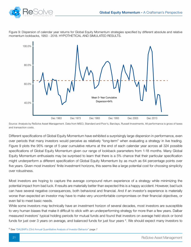
Figure 9: Dispersion of calendar year returns for Global Equity Momentum strategies specified by different absolute and relative momentum lookbacks, 1950 - 2018. HYPOTHETICAL AND SIMULATED RESULTS.

Mean 5−Year CumulativeDispersion=64%40.0%

60.0%

80.0%

100.0%

Dec 1963 Dec 1973 Dec 1983 Dec 1993 Dec 2003 Dec 2013



Different specifications of Global Equity Momentum have exhibited a surprisingly large dispersion in performance, even over periods that many investors would perceive as relatively “long-term” when evaluating a strategy in live trading. Figure 9 plots the 95% range of 5-year cumulative returns at the end of each calendar year across all 324 possible specifications of Global Equity Momentum given our range of lookback parameters from 1-18 months. Many Global Equity Momentum enthusiasts may be surprised to learn that there is a 5% chance that their particular specification might underperform a different specification of Global Equity Momentum by as much as 64 percentage points over five years. Given most investors’ finite investment horizons, this seems like a large potential cost for choosing simplicity over robustness.

Most investors are hoping to capture the average compound return experience of a strategy while minimizing the potential impact from bad luck. If results are materially better than expected this is a happy accident. However, bad luck can have several negative consequences, both behavioral and financial. And if an investor’s experience is materially worse than expected an investor may have to make very uncomfortable compromises on their financial objectives, or even fail to meet basic needs.While some investors may technically have an investment horizon of several decades, most investors are susceptible to very human biases that make it difficult to stick with an underperforming strategy for more than a few years. Dalbar measured investors’ typical holding periods for mutual funds and found that investors on average held stock or bond funds for just over 3 years on average, and balanced funds for just four years 6. We should expect many investors to

6 See “DALBAR’s 23rd Annual Quantitative Analysis of Investor Behavior” page 7

https://svwealth.com/wp-content/uploads/2018/04/dalbar_study.pdf



abandon other investment strategies after three or perhaps five years of underperformance relative to expectations.

Investors who are able to weather many years of underperformance may still face unpalatable financial consequences. Aside from the possibility of drawing a sample of low average returns, investors may also experience an unlucky sequence of returns. Investors with cash flows like savers, retirees, or distributing institutions need to be concerned with both the average and the sequence of their returns. It is unhelpful for savers to experience high returns early in their career when they have less capital invested, only to realize low returns late in their career when they are all cashed up. A retiree is especially vulnerable to low returns immediately before, and for the decade after retirement. High returns late in retirement are irrelevant since the investor will have almost depleted his or her funds.

We can measure the concept of stability from a few different angles. For example, we can examine the range of historical outcomes over rolling five- or ten-year periods. We can observe the performance of the strategy if an investor had failed to capture a small sample of the best monthly returns. And we can examine the expected return of an investor who experiences a below-average return path.

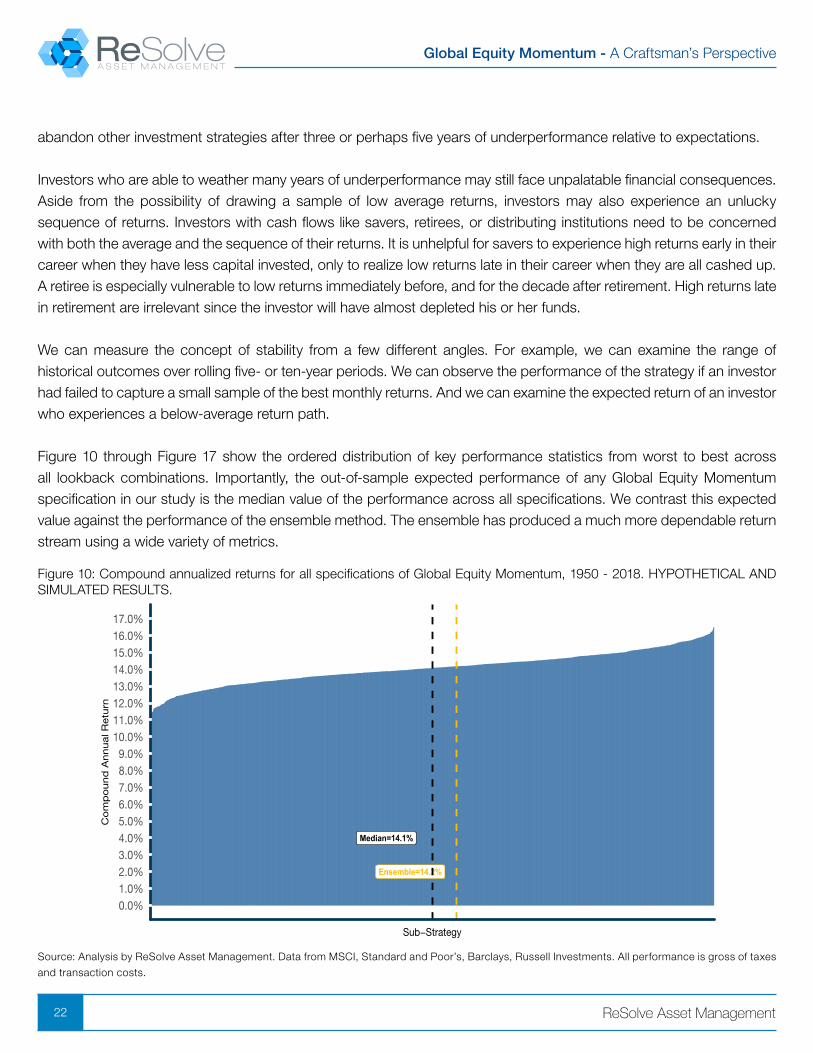
Figure 10 through Figure 17 show the ordered distribution of key performance statistics from worst to best across all lookback combinations. Importantly, the out-of-sample expected performance of any Global Equity Momentum specification in our study is the median value of the performance across all specifications. We contrast this expected value against the performance of the ensemble method. The ensemble has produced a much more dependable return stream using a wide variety of metrics.

Figure 10: Compound annualized returns for all specifications of Global Equity Momentum, 1950 - 2018. HYPOTHETICAL AND SIMULATED RESULTS.

Ensemble=14.2%

Median=14.1%

0.0%1.0%2.0%3.0%4.0%5.0%6.0%7.0%8.0%9.0%

10.0%11.0%12.0%13.0%14.0%15.0%16.0%17.0%

Sub−Strategy

Co

mp

ound

Annual R

etu

rn





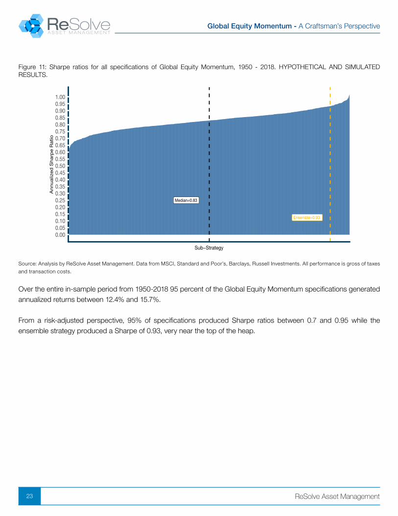
Figure 11: Sharpe ratios for all specifications of Global Equity Momentum, 1950 - 2018. HYPOTHETICAL AND SIMULATED RESULTS.

Ensemble=0.93

Median=0.83

0.000.050.100.150.200.250.300.350.400.450.500.550.600.650.700.750.800.850.900.951.00

Sub−Strategy

Annualiz

ed

Sharp

e R

atio



Over the entire in-sample period from 1950-2018 95 percent of the Global Equity Momentum specifications generated annualized returns between 12.4% and 15.7%.

From a risk-adjusted perspective, 95% of specifications produced Sharpe ratios between 0.7 and 0.95 while the ensemble strategy produced a Sharpe of 0.93, very near the top of the heap.



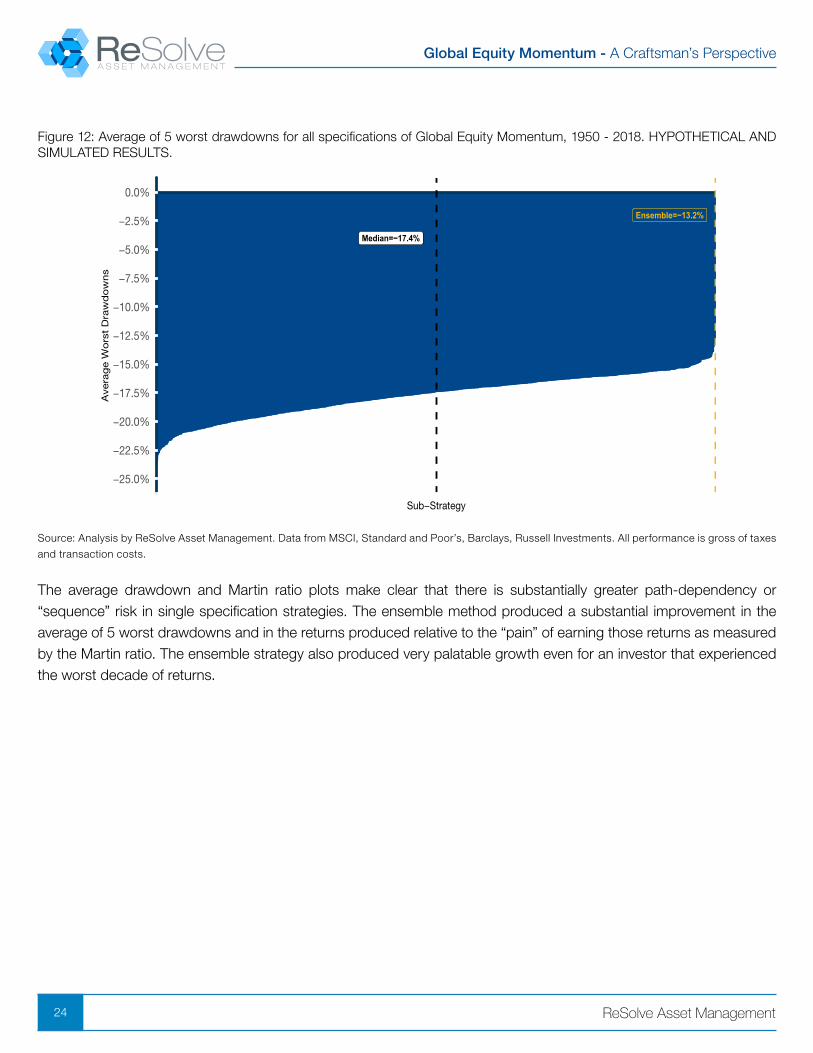
Figure 12: Average of 5 worst drawdowns for all specifications of Global Equity Momentum, 1950 - 2018. HYPOTHETICAL AND SIMULATED RESULTS.

Ensemble=−13.2%

Median=−17.4%

−25.0%

−22.5%

−20.0%

−17.5%

−15.0%

−12.5%

−10.0%

−7.5%

−5.0%

−2.5%

0.0%

Sub−Strategy

Ave

rag

e W

ors

t D

raw

do

wns



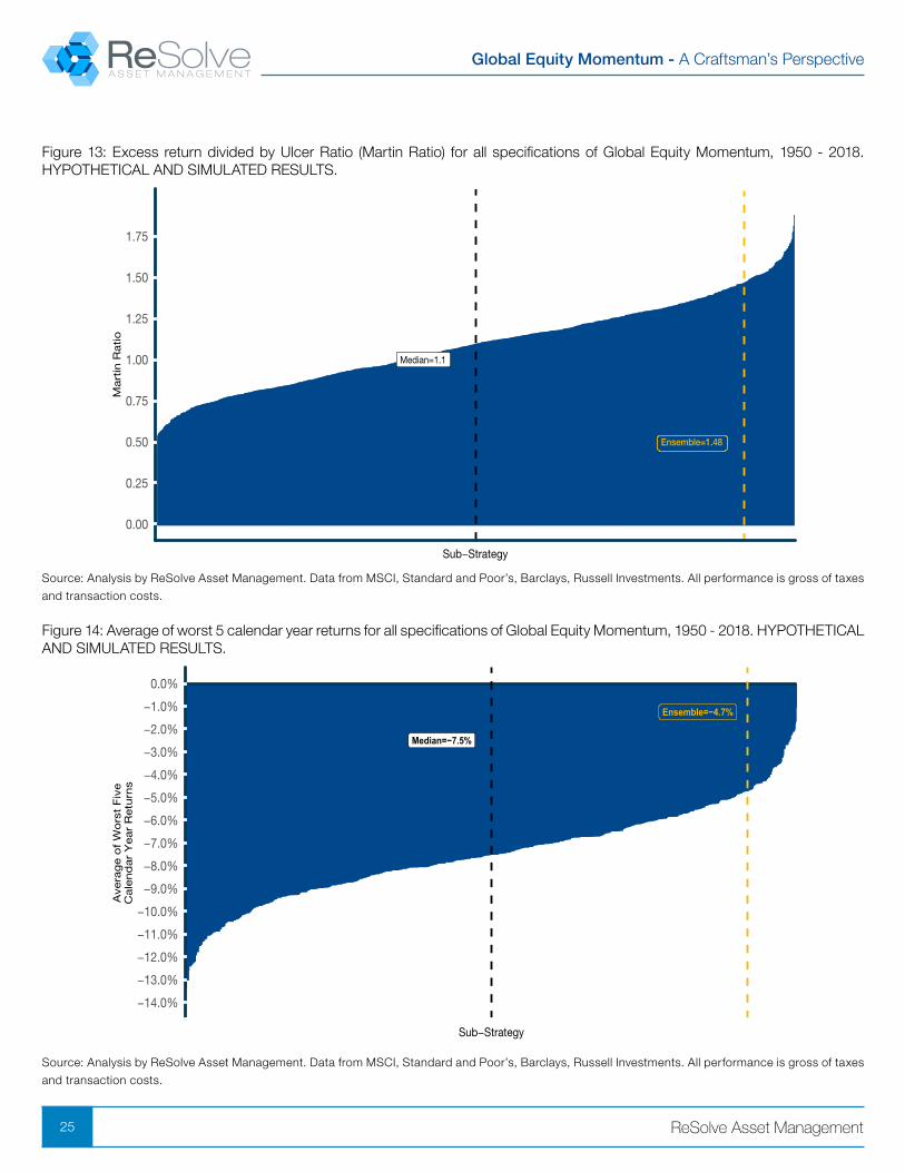
The average drawdown and Martin ratio plots make clear that there is substantially greater path-dependency or “sequence” risk in single specification strategies. The ensemble method produced a substantial improvement in the average of 5 worst drawdowns and in the returns produced relative to the “pain” of earning those returns as measured by the Martin ratio. The ensemble strategy also produced very palatable growth even for an investor that experienced the worst decade of returns.



Figure 13: Excess return divided by Ulcer Ratio (Martin Ratio) for all specifications of Global Equity Momentum, 1950 - 2018. HYPOTHETICAL AND SIMULATED RESULTS.

Ensemble=1.48

Median=1.1

0.00

0.25

0.50

0.75

1.00

1.25

1.50

1.75

Sub−Strategy

Mart

in R

atio



Figure 14: Average of worst 5 calendar year returns for all specifications of Global Equity Momentum, 1950 - 2018. HYPOTHETICAL AND SIMULATED RESULTS.

Ensemble=−4.7%

Median=−7.5%

−14.0%

−13.0%

−12.0%

−11.0%

−10.0%

−9.0%

−8.0%

−7.0%

−6.0%

−5.0%

−4.0%

−3.0%

−2.0%

−1.0%

0.0%

Sub−Strategy

Ave

rag

e o

f W

ors

t F

ive

Cale

nd

ar

Year

Retu

rns





Figure 15: Total returns in worst decade for all specifications of Global Equity Momentum, 1950 - 2018. HYPOTHETICAL AND SIMULATED RESULTS.

Ensemble=90.1%

Median=72.1%

0%

10%

20%

30%

40%

50%

60%

70%

80%

90%

100%

110%

120%

130%

140%

150%

160%

Sub−Strategy

Wo

rst

Decad

e T

ota

l Retu

rn

Source: Analysis by ReSolve Asset Management. Data from MSCI, Standard and Poor’s, Barclays, Russell Investments. All performance is gross of taxes and transaction costs.

Figure 16: Compound annualized returns without the best 5% of monthly returns for all specifications of Global Equity Momentum, 1950 - 2018. HYPOTHETICAL AND SIMULATED RESULTS.

Ensemble=9.8%

Median=9.1%

0.0%

10.0%

Sub−Strategy

Annualiz

ed

Retu

rn If

Yo

uM

iss

To

p 5

% o

f M

onth

s

Source: Analysis by ReSolve Asset Management. Data from MSCI, Standard and Poor’s, Barclays, Russell Investments.. All performance is gross of taxes




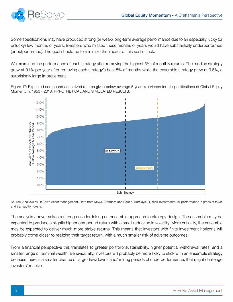
Some specifications may have produced strong (or weak) long-term average performance due to an especially lucky (or unlucky) few months or years. Investors who missed these months or years would have substantially underperformed (or outperformed). The goal should be to minimize the impact of this sort of luck.

We examined the performance of each strategy after removing the highest 5% of monthly returns. The median strategy grew at 9.1% per year after removing each strategy’s best 5% of months while the ensemble strategy grew at 9.8%, a surprisingly large improvement.

Figure 17: Expected compound annualized returns given below average 5 year experience for all specifications of Global Equity Momentum, 1950 - 2018. HYPOTHETICAL AND SIMULATED RESULTS.

Ensemble=9.8%

Median=9.3%

0.0%

1.0%

2.0%

3.0%

4.0%

5.0%

6.0%

7.0%

8.0%

9.0%

10.0%

11.0%

12.0%

Sub−Strategy

Annualiz

ed

Exp

ecte

d R

etu

rn f

or

Belo

w A

vera

ge 5

Year

Perio

d



The analysis above makes a strong case for taking an ensemble approach to strategy design. The ensemble may be expected to produce a slightly higher compound return with a small reduction in volatility. More critically, the ensemble may be expected to deliver much more stable returns. This means that investors with finite investment horizons will probably come closer to realizing their target return, with a much smaller risk of adverse outcomes.

From a financial perspective this translates to greater portfolio sustainability, higher potential withdrawal rates, and a smaller range of terminal wealth. Behaviourally, investors will probably be more likely to stick with an ensemble strategy because there is a smaller chance of large drawdowns and/or long periods of underperformance, that might challenge investors’ resolve.



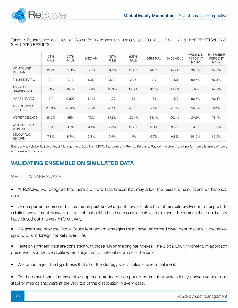
Table 1: Performance quantiles for Global Equity Momentum strategy specifications, 1950 - 2018. HYPOTHETICAL AND SIMULATED RESULTS.

5TH %ILE

25TH %ILE

MEDIAN75TH %ILE

95TH %ILE

ORIGINAL ENSEMBLEORIGINAL PERCENT

RANK

ENSEMBLE PERCENT

RANK

COMPOUND RETURN

12.4% 13.4% 14.1% 14.7% 15.7% 14.9% 14.2% 80.8% 54.3%

SHARPE RATIO 0.7 0.78 0.83 0.88 0.95 0.9 0.93 82.7% 93.1%

AVG MAX DRAWDOWN

21% 19.1% 17.4% 16.3% 15.3% 16.5% 13.2% 69% 99.9%

MARTIN RATIO 0.7 0.892 1.103 1.29 1.531 1.351 1.477 82.7% 92.1%

AVG OF WORST 5 YEARS

-10.9% -8.8% -7.5% -6.1% -4.3% -7% -4.7% 59.5% 92%

WORST DECADE 35.3% 55% 72% 87.6% 120.4% 55.1% 90.1% 25.1% 78.4%

WITHOUT BEST MONTHS

7.5% 8.5% 9.1% 9.8% 10.7% 9.8% 9.8% 76% 76.7%

BELOW AVG RETURN

7.8% 8.7% 9.3% 9.9% 11% 9.7% 9.8% 66.9% 69.9%



VALIDATING ENSEMBLE ON SIMULATED DATA

SECTION TAKEAWAYS

• At ReSolve, we recognize that there are many tacit biases that may affect the results of simulations on historical data.

• One important source of bias is the ex post knowledge of how the structure of markets evolved in retrospect. In addition, we are acutely aware of the fact that political and economic events are emergent phenomena that could easily have played out in a very different way.

• We examined how the Global Equity Momentum strategies might have performed given perturbations in the make-up of U.S. and foreign markets over time.

• Tests on synthetic data are consistent with those run on the original indexes. The Global Equity Momentum approach preserved its attractive profile when subjected to material return perturbations.

• We cannot reject the hypothesis that all of the strategy specifications have equal merit.

• On the other hand, the ensemble approach produced compound returns that were slightly above average, and stability metrics that were at the very top of the distribution in every case.



Many analysts might feel satisfied with the conclusions derived from the analyses presented in the previous sections. At ReSolve, we recognize that there are many tacit biases that may affect the results of simulations on historical data.One important source of bias is the ex post knowledge of how the structure of markets evolved in retrospect. For example, while it is obvious looking back that markets evolved so that about half of equity market capitalization accrued to U.S. markets and about half accrued to foreign markets, this was not an obvious distinction at various points in time between 1950 and today.

In addition, we are acutely aware of the fact that political and economic events are emergent phenomena that could easily have played out in a very different way. Accumulated small differences in outcomes along the arc of history would have compounded to produce a potentially unrecognizable economic and/or political environment today.

With this awareness, we felt motivated to examine how the Global Equity Momentum strategies might have performed given perturbations in the make-up of U.S. and foreign markets over time. This type of analysis provides greater insight into the potential distribution of outcomes for a Global Equity Momentum strategy going forward. We also have an opportunity to observe the power of the ensemble strategy in a somewhat “out-of-sample” context.

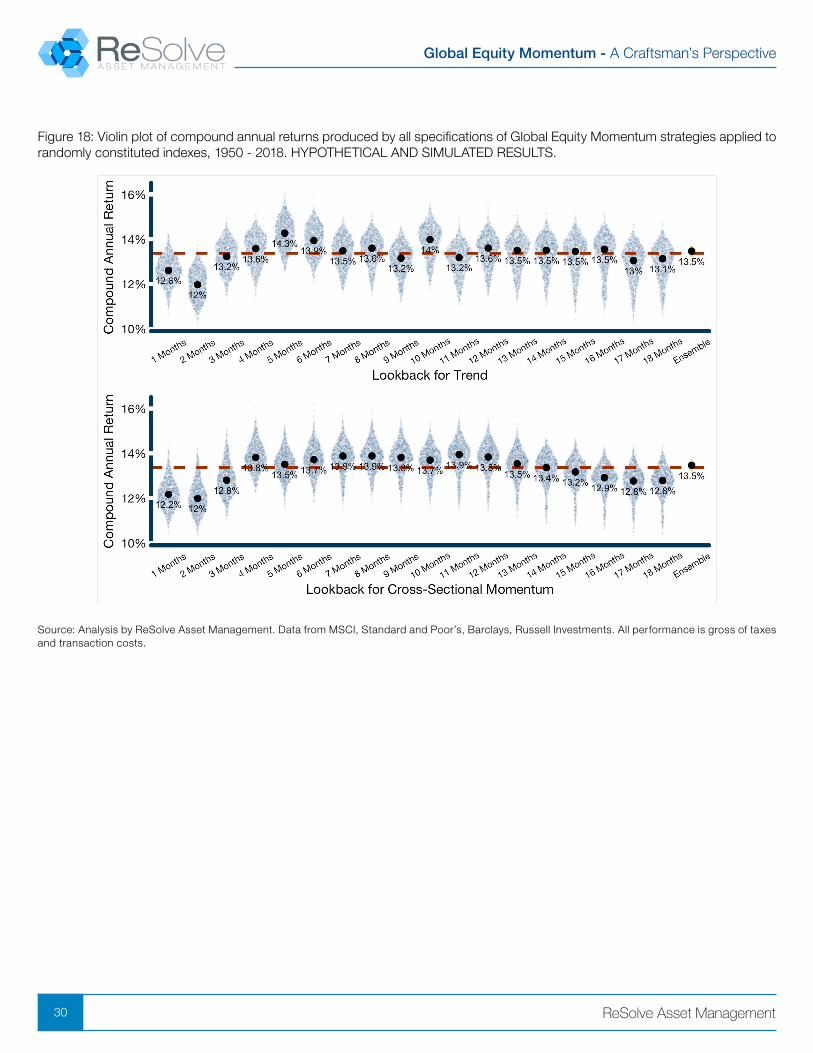
The following plots are generated by applying the traditional time-series momentum approach to Global Equity Momentum across all cross-sectional and trend lookback lengths from 1-18 months.

We created 1000 synthetic return series for both foreign stocks and US stocks. Each synthetic series preserved the time continuity of the original market returns. To manufacture synthetic series of foreign stocks we created random portfolios of individual developed ex-US markets (i.e. German stocks, French stocks, Japanese stocks, etc.) and found the monthly returns of the random portfolios. We averaged those returns with the monthly returns of our primary foreign equity index to create our synthetic foreign index for each sample.

For US stocks we created random portfolios of returns from major US equity indexes from Russell, MSCI and S&P as well as style indexes (growth and value) and sector indexes. We averaged the monthly returns from the random portfolios with S&P returns to create our synthetic US index for each sample.For each synthetic index we ran Global Equity Momentum strategies for all 324 traditional time-series specifications for a total of 324 thousand simulations in total.

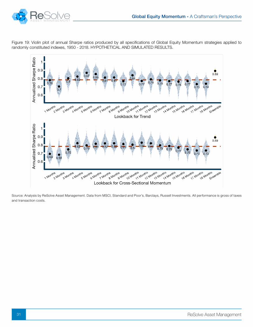
The violin plots below show the distribution of key summary performance statistics sorted on momentum and trend lookbacks independently against the distribution of outcomes from all ensembles. There are 18 thousand points for each independent lookback of trend and momentum and 1 ensemble for each sample for a total of 1000 ensembles.



Figure 18: Violin plot of compound annual returns produced by all specifications of Global Equity Momentum strategies applied to randomly constituted indexes, 1950 - 2018. HYPOTHETICAL AND SIMULATED RESULTS.

Source: Analysis by ReSolve Asset Management. Data from MSCI, Standard and Poor’s, Barclays, Russell Investments. All performance is gross of taxes and transaction costs.



Figure 19: Violin plot of annual Sharpe ratios produced by all specifications of Global Equity Momentum strategies applied to randomly constituted indexes, 1950 - 2018. HYPOTHETICAL AND SIMULATED RESULTS.





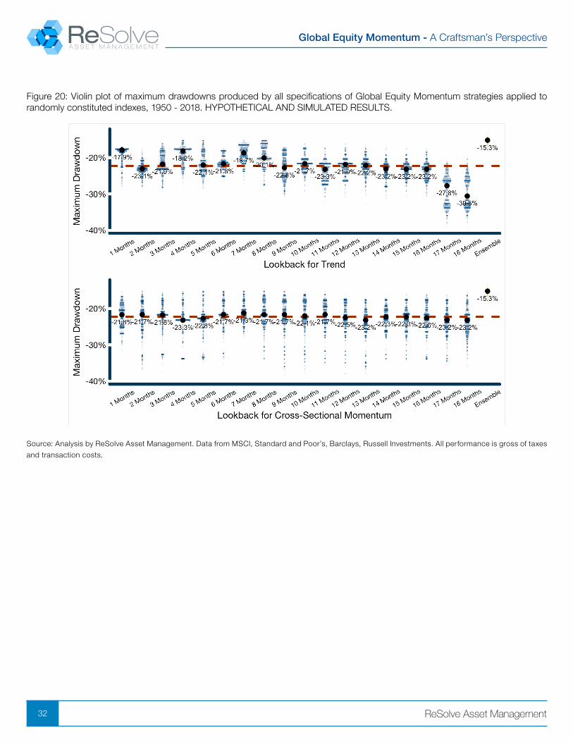
Figure 20: Violin plot of maximum drawdowns produced by all specifications of Global Equity Momentum strategies applied to randomly constituted indexes, 1950 - 2018. HYPOTHETICAL AND SIMULATED RESULTS.





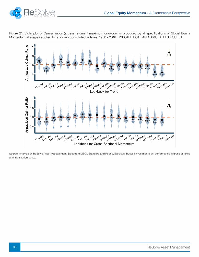
Figure 21: Violin plot of Calmar ratios (excess returns / maximum drawdowns) produced by all specifications of Global Equity Momentum strategies applied to randomly constituted indexes, 1950 - 2018. HYPOTHETICAL AND SIMULATED RESULTS.





Tests on synthetic data are consistent with those run on the original indexes. The Global Equity Momentum approach preserved its attractive profile when subjected to material return perturbations.While there is some dispersion in results for strategies specified with different lookbacks for absolute and relative momentum, all of the violin plots show a substantial amount of overlap. We cannot reject the hypothesis that all of the strategy specifications have equal merit.

On the other hand, the ensemble approach produced compound returns that were slightly above average, and stability metrics that were at the very top of the distribution in every case. We perceive this as very strong validation of the case for an ensemble approach.

TAX DISCUSSION

SECTION TAKEAWAYS

• The Original strategy specification trades relatively infrequently and produces mostly long-term gains for tax purposes.

• The ensemble strategy trades much more frequently and nets a larger proportion of short-term gains.

• We estimate that taxes reduced the returns on the Original specification by approximately 3% per year while the ensemble reduced returns by 3.5% per year due to taxes.

• However, tailwinds from rebalancing effects and a reduction in volatility drag reduce the difference in expected tax costs to 0.3% per year.

Note that trading any single specification requires that 200% of the portfolio be rebalanced on a signal change, i.e. the complete sale of one market and purchase of another market. Longer-term specifications may trade less often, but changes are more dramatic for what is often a very small change in signal. So they suffer from large specification risk and the potential for large tax impacts on potentially very small changes in market conditions.

The ensemble strategy makes smaller trades more often, reflecting small incremental changes in market conditions. It minimizes specification risk and will rarely require large portfolio changes, but requires a larger operational burden.The ensemble Global Equity Momentum strategy realized 1867 trades versus 105 trades for the Original specification. And while almost 70 percent of profits from the Original specification were subject to long-term capital gains, the ensemble method crystallized a large proportion of short-term gains.

However, for tax purposes it is important to examine the distribution of short-term losses versus short-term gains. Momentum and trend can be summarized as strategies that “cut losses short but let winners run”. They tend to crystallize many small short-term losses while realizing a small number of large long-term gains. This is very attractive since short-term losses add up more quickly and can be deployed to buttress future long-term gains.



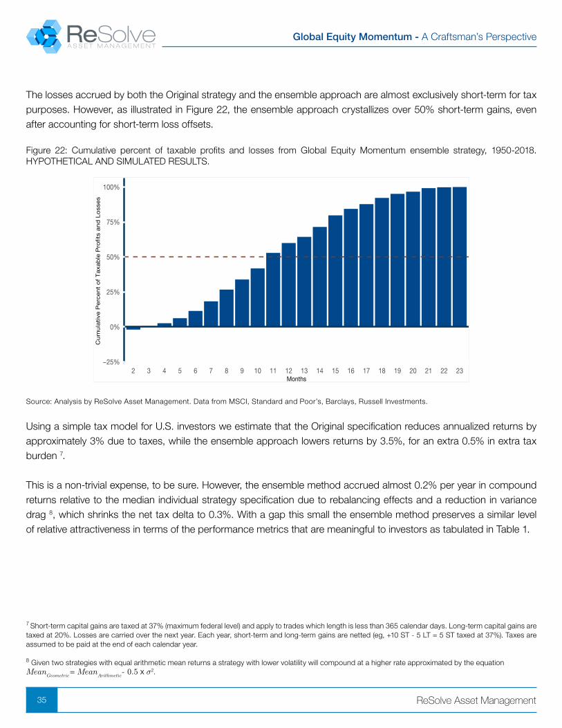
The losses accrued by both the Original strategy and the ensemble approach are almost exclusively short-term for tax purposes. However, as illustrated in Figure 22, the ensemble approach crystallizes over 50% short-term gains, even after accounting for short-term loss offsets.

Figure 22: Cumulative percent of taxable profits and losses from Global Equity Momentum ensemble strategy, 1950-2018. HYPOTHETICAL AND SIMULATED RESULTS.

−25%

0%

25%

50%

75%

100%

2 3 4 5 6 7 8 9 10 11 12 13 14 15 16 17 18 19 20 21 22 23Months

Cum

ula

tive

Perc

ent

of

Taxab

le P

ro�ts

and

Lo

sses

Source: Analysis by ReSolve Asset Management. Data from MSCI, Standard and Poor’s, Barclays, Russell Investments.

Using a simple tax model for U.S. investors we estimate that the Original specification reduces annualized returns by approximately 3% due to taxes, while the ensemble approach lowers returns by 3.5%, for an extra 0.5% in extra tax burden 7.

This is a non-trivial expense, to be sure. However, the ensemble method accrued almost 0.2% per year in compound returns relative to the median individual strategy specification due to rebalancing effects and a reduction in variance drag 8, which shrinks the net tax delta to 0.3%. With a gap this small the ensemble method preserves a similar level of relative attractiveness in terms of the performance metrics that are meaningful to investors as tabulated in Table 1.

7 Short-term capital gains are taxed at 37% (maximum federal level) and apply to trades which length is less than 365 calendar days. Long-term capital gains are taxed at 20%. Losses are carried over the next year. Each year, short-term and long-term gains are netted (eg, +10 ST - 5 LT = 5 ST taxed at 37%). Taxes are assumed to be paid at the end of each calendar year.

8 Given two strategies with equal arithmetic mean returns a strategy with lower volatility will compound at a higher rate approximated by the equation Mean

Geometric = Mean

Arithmetic- 0.5 x ¾ 2.



CRAFTSMANSHIP TAX ALPHA

SECTION TAKEAWAYS

• A Global Equity Momentum strategy would be expected to produce a substantial amount of trading due purely to noisy signals.

• The ensemble approach includes some very short-term lookback horizons that will create a larger amount of noise trades.• We created a model to estimate the amount of trading we should expect from the ensemble strategy based purely on noise.

• We imposed a threshold on trades in the ensemble model so that we expect to eliminate 95% of noise trading.

• This approach almost completely closes the tax gap between the Original specification and the ensemble approach.

• On an after-tax basis the ensemble approach with intelligent trade management preserves the performance benefits of the pre-tax version.

Trend and momentum signals are very noisy especially at the shorter lookback horizons, and this generates material unproductive trading. Our objective should be to filter out trades produced by noise so that we only trade when the strategy requires meaningful changes to the portfolio.

We investigated how much trading we should expect from one month to the next purely on the basis of random noise. We ran the Global Equity Momentum strategy on 1000 row-wise bootstrap samples of the detrended individual market returns to see how much trading was required. This method preserved the pairwise correlations and empirical return distribution while eliminating drift and trend effects, so it is essentially a correlated white noise process 9.The average absolute monthly sum of differences in portfolio weights was 35% and the 95th percentile was 40%. From this we inferred that we need to see greater than 40% absolute sum of differences in portfolio weights to be at least 95% certain that the changes are not simply due to random noise.

Following this logic, we implemented a rule where we only trade when the absolute sum of differences in weights between one month and the next exceeds 40 percent. Otherwise we kept the previous weights for the current month.

This trade management strategy reduced the total number of trades for the ensemble from 1867 to 900, a reduction of more than 50 percent. More importantly, almost two-thirds of net profits accrued from long-term capital gains, such that the total excess tax burden from the ensemble approach was reduced to just 6 basis points in excess of the Original

9 We ran similar tests preserving the historical mean return for each market, and other tests based on pure white noise with zero mean and volatility of 20% for each stock series with 5% for the bond series. All of our tests yielded similar results.



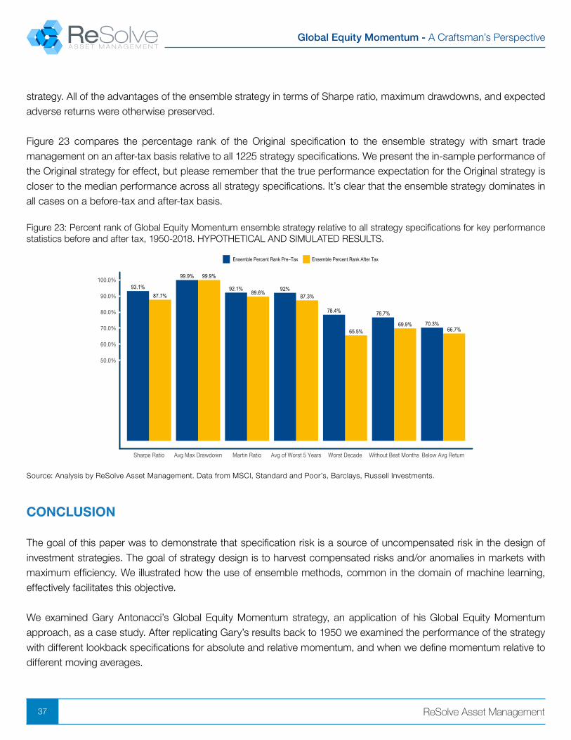
strategy. All of the advantages of the ensemble strategy in terms of Sharpe ratio, maximum drawdowns, and expected adverse returns were otherwise preserved.

Figure 23 compares the percentage rank of the Original specification to the ensemble strategy with smart trade management on an after-tax basis relative to all 1225 strategy specifications. We present the in-sample performance of the Original strategy for effect, but please remember that the true performance expectation for the Original strategy is closer to the median performance across all strategy specifications. It’s clear that the ensemble strategy dominates in all cases on a before-tax and after-tax basis.

Figure 23: Percent rank of Global Equity Momentum ensemble strategy relative to all strategy specifications for key performance statistics before and after tax, 1950-2018. HYPOTHETICAL AND SIMULATED RESULTS.

87.7%93.1%

99.9%99.9%

89.6%92.1%

87.3%92%

65.5%

78.4%

69.9%

76.7%

66.7%70.3%

50.0%

60.0%

70.0%

80.0%

90.0%

100.0%

Sharpe Ratio Avg Max Drawdown Martin Ratio Avg of Worst 5 Years Worst Decade Without Best Months Below Avg Return

Ensemble Percent Rank Pre−Tax Ensemble Percent Rank After Tax

Source: Analysis by ReSolve Asset Management. Data from MSCI, Standard and Poor’s, Barclays, Russell Investments.

CONCLUSION

The goal of this paper was to demonstrate that specification risk is a source of uncompensated risk in the design of investment strategies. The goal of strategy design is to harvest compensated risks and/or anomalies in markets with maximum efficiency. We illustrated how the use of ensemble methods, common in the domain of machine learning, effectively facilitates this objective.

We examined Gary Antonacci’s Global Equity Momentum strategy, an application of his Global Equity Momentum approach, as a case study. After replicating Gary’s results back to 1950 we examined the performance of the strategy with different lookback specifications for absolute and relative momentum, and when we define momentum relative to different moving averages.



We performed robust statistical tests to determine whether the Original specification is superior to other specifications with a reasonable level of confidence and concluded that this approach is just one of many equally valid specifications.Since all specifications have equal merit, we make the case that the best estimate for the expected performance of any individual strategy specification – including the Original specification - is the median across all specifications.

Next we introduced the concept of an ensemble strategy and referenced some machine learning articles that showed how ensembles have been used effectively to win many competitions. The ensemble takes advantage of the fact that each individual specification has similar expected performance, but that they will produce errors at different times. By making use of signals from all individual specifications the ensemble can capture the essence of the underlying “styles” with less noise than any individual specification.

We showed empirically that the ensemble produced more stable returns, with less vulnerability to extreme outlier events. In other words, the ensemble provided the average investor an experience that was closest to their expectations over finite time horizons, with much lower probability of major adverse outcomes. We validated this conclusion using a large bootstrap of synthetic data modeled on the original data.

Finally we examined the profile of the ensemble strategy relative to the Original specification on an after-tax basis. The ensemble produced over 10 times more trades and accrued an extra 0.5% in excess tax “costs”.

Many of the underlying strategies are based on short-term signals, which are inherently noisy. We set out to minimize trading on random signals, and performed a simulation on white noise with similar amplitude as the underlying markets to determine how much turnover we would expect from month to month trading on random data. We set a trading threshold based on the 95th percentile of expected turnover derived from our simulation, and analyzed the impacts on trade count and taxes. Our trade management strategy reduced turnover by more than 50% and almost completely eliminated the excess tax consequences from trading the ensemble strategy.

When the direct source of an edge is hidden from view, the best we can hope is to capture a portion of the signal with any single specification. Ensembles view an endogenous investment edge from many perspectives. Just as two eyes provide perspective to our visual senses, and Array Radio Telescopes provide an unparalleled view of the universe by combining signals from many small dishes, ensembles provide greater resolution of investment signals to produce a more stable investment experience.



Disclaimer

Confidential and proprietary information. The contents hereof may not be reproduced or disseminated without the express written permission of

ReSolve Asset Management Inc. (“ReSolve”). ReSolve is registered as an investment fund manager in Ontario and Newfoundland and Labrador, and as

a portfolio manager and exempt market dealer in Ontario, Alberta, British Columbia and Newfoundland and Labrador. As well as a Commodity Trading

Manager in Ontario. Additionally, ReSolve is an SEC registered investment adviser.

ReSolve is also registered with the Commodity Futures Trading Commission as a commodity trading advisor and a Commodity Pool Operator. This

registration is administered through the National Futures Association (“NFA”). Certain of ReSolve’s employees are registered with the NFA as Principals

and/or Associated Persons of ReSolve if necessary or appropriate to perform their responsibilities. ReSolve has claimed an exemption under CFTC Rule

4.7 which exempts Resolve from certain part 4 requirements with respect to offerings to qualified eligible persons.

PAST PERFORMANCE IS NOT NECESSARILY INDICATIVE OF FUTURE RESULTS

This presentation does not constitute an offer to sell or a solicitation of interest to purchase any securities or investment advisory services in any

jurisdiction in which such offer or solicitation is not authorized.

Forward-Looking Information. This presentation may contain “forward-looking information. Because such forward-looking information involves risks

and uncertainties, actual results of the funds or accounts may differ materially from any expectations, projections or predictions made or implicated in

such forward-looking information. Prospective investors are therefore cautioned not to place undue reliance on such forward-looking statements. In

addition, in considering any prior performance information contained in this presentation, prospective investors should bear in mind that past results

are not necessarily indicative of future results, and there can be no assurance that the funds or any account will achieve results comparable to those

discussed in this presentation. This presentation speaks as of the date hereof and neither ReSolve nor any affiliate or representative thereof assumes any

obligation to provide any recipient of this presentation with subsequent revisions or updates to any historical or forward-looking information contained in

this presentation to reflect the occurrence of events and/or changes in circumstances after the date hereof.

General information regarding hypothetical performance and simulated results. Past results are not necessarily indicative of future results. It

is expected that the simulated performance will periodically change as a function of both refinements to our simulation methodology and the underlying

market data. These results are based on simulated or hypothetical performance results that have certain inherent limitations. Unlike the results in an actual

performance record, these results do not represent actual trading. Also, because these trades have not actually been executed, these results may have

under- or over-compensated for the impact, if any, of certain market factors, such as lack of liquidity. Simulated or hypothetical trading programs in general

are also subject to the fact that they are designed with the benefit of hindsight. No representation is being made that any account or fund will or is likely

to achieve profits or losses similar to those being shown. The results do not include other costs of managing a portfolio (such as custodial fees, legal,

auditing, administrative or other professional fees). The information in this presentation has not been reviewed or audited by an independent accountant

or other independent testing firm. More detailed information regarding the manner in which the charts were calculated is available on request. Any actual

fund or account that ReSolve manages will invest in different economic conditions, during periods with different volatility and in different securities than

those incorporated in the hypothetical performance charts shown. There is no representation that any fund or account will perform as the hypothetical or

other performance charts indicate.

global equity momentum - investresolve.com · global equity momentum - a raftsman’s erspective 7...

Documents