Global Flood Modelling:Statistical Estimation of Peak-Flow Magnitude

World Bank Development Research Group &

UNEP/GRID-Europe Early Warning Unit

Christian HEROLD, GIS-AnalystUNEP/GRID-EuropeChristian.Herold@grid.unep.chDr Frédéric MOUTON, StatisticianUniversity of Geneva (Switzerland), Math.and University of Grenoble (France), InstitutFrederic.Mouton@fourier.ujf-grenoble.fr

February 2006

UNEP/GRID-Europe 11, ch. Des Anémones 1219 Châtelaine Geneva – Switzerland Tel: +4122.917.82.94 Fax: +4122.917.80.29 Website: www.grid.unep.ch

Lead Authors Christian Herold and Frédéric Mouton

Citation Herold, C., F. Mouton, (2006), Global Flood Modelling, Statistical Estimation of Peak-Flow Magnitude, World Bank Development Research Group - UNEP/GRID-Europe.

© UNEP - World Bank 2006

Disclaimer The designations employed and the presentation of material on the maps do not imply the expression of any opinion whatsoever on the part of UNEP or the Secretariat of the United Nations concerning the legal status of any country, territory, city or area or of its authorities, or concerning the delimitation of its frontiers or boundaries. This analysis was conducted using global data sets, the resolution of which is not suitable for in-situ planning. UNEP and collaborators should in no case be liable for misuse of the presented results. The views expressed in this publication are those of the authors and do not necessarily reflect those of UNEP.

Acknowledgements This work was supported by the World Bank through the Swiss Consultant Trust Fund. We would like to thanks the following persons who gave us the opportunity to work on this project and have collaborated directly or indirectly to this preliminary research: Uwe Deichmann, Piet Buys, Maxx Dilley, Gregory Yetman, James P. Verdin, Kristine L. Verdin, Kwabena Asante, Charles J. Vörösmarty, Upmanu Lall, Emily Grover-Kopek, Randy Pullen, Pascal Peduzzi, Stéphane Kluser. .

Abstract The scope of the present paper is to describe an exploratory analysis on the feasibility of a global flood hazard modeling, which would enable further studies on human vulnerability The method chosen is inspired by local peak-flow magnitude estimations realized in the U.S. After determining -by GIS-processing- for each HYDRO1k level 4 basin a set of hydromorphometric and climatic values and the coordinates of a corresponding gauged or ungauged outlet station, peak flow magnitude for gauged stations are estimated using log-Pearson type III distribution, following the directions of Bulletin 17B from USWRC’s Hydrologic Subcommittee. Estimates of peak-flow magnitude for ungauged stations are then obtained by statistical means, performing several regressions on the basin variables. Peak-flow magnitude estimates enable the computation of corresponding flooded areas using Manning’s equation and GISprocessing. This “regression method” is processed on two test-zones situated in North and South America.

i

Table of Contents Abstract......................................................................................................1 Acknowledgements ...................................................................................1 1 Introduction........................................................................................1

1.1 Project definition............................................................................................1 1.2 Choice of a global method .............................................................................1 1.3 Definition of Peak Flow.................................................................................2

2 GIS-Processing ...................................................................................2 2.1 Discharge stations dataset. .............................................................................2 2.2 Variables used for peak flow estimation........................................................3

2.2.1 Hydromorphometric and Land cover variables. ....................................3 2.2.2 Climatic variables. .................................................................................4 2.2.3 Climatic zones........................................................................................5

3 Statistical Analysis .............................................................................5 3.1 Peak-flow values for gauging stations. ..........................................................6 3.2 Transformation of variables...........................................................................6 3.3 Descriptive analysis for North American gauging stations ...........................7 3.4 Groups, regressions and predictions ..............................................................7

4 Flooded area estimation ....................................................................8 4.1 Manning’s equation .......................................................................................8 4.2 GIS-processing...............................................................................................8 4.3 Calibration......................................................................................................9

5 First test zone: North America .........................................................9 5.1 GIS-processing.............................................................................................10 5.2 Composition of groups.................................................................................11 5.3 Regression formulae. ...................................................................................12 5.4 Peak-flow values for ungauged sites............................................................13 5.5 Flooded area estimations..............................................................................14

6 Second test zone: South America ...................................................14 6.1 GIS-processing.............................................................................................15 6.2 Composition of groups.................................................................................15 6.3 Cross-validation between South and North America...................................16 6.4 Test of the PLS regression ...........................................................................19 6.5 Final regressions ..........................................................................................20 6.6 Flooded area estimations..............................................................................20

7 Remarks and recommendations for further studies ....................21 7.1 Data. .............................................................................................................21

7.1.1 SRTM and HYDRO1k.........................................................................21 7.1.2 Climatic variables. ...............................................................................21 7.1.3 Soil characteristics. ..............................................................................21

7.2 GIS-processing.............................................................................................21 7.2.1 GRDC stations spatial selection...........................................................21 7.2.2 Main channel........................................................................................21 7.2.3 Manning’s equation and discharge vs. stage rating curves..................21

ii

7.3 Statistical analysis........................................................................................22 7.3.1 Composition of groups.........................................................................22 7.3.2 Regressions ..........................................................................................22 7.3.3 Validations ...........................................................................................22

8 Conclusion.........................................................................................22 9 Appendixes........................................................................................23

1

Abstract The scope of the present paper is to describe an exploratory analysis on the feasibility of a global flood hazard modeling, which would enable further studies on human vulnerability The method chosen is inspired by local peak-flow magnitude estimations realized in the U.S. After determining -by GIS-processing- for each HYDRO1k level 4 basin a set of hydromorphometric and climatic values and the coordinates of a corresponding gauged or ungauged outlet station, peak flow magnitude for gauged stations are estimated using log-Pearson type III distribution, following the directions of Bulletin 17B from USWRC’s Hydrologic Subcommittee. Estimates of peak-flow magnitude for ungauged stations are then obtained by statistical means, performing several regressions on the basin variables. Peak-flow magnitude estimates enable the computation of corresponding flooded areas using Manning’s equation and GIS-processing. This “regression method” is processed on two test-zones situated in North and South America. Acknowledgements This work was supported by the World Bank through the Swiss Consultant Trust Fund. We would like to thanks the following persons who gave us the opportunity to work on this project and have collaborated directly or indirectly to this preliminary research: Uwe Deichmann, Piet Buys, Maxx Dilley, Gregory Yetman, James P. Verdin, Kristine L. Verdin, Kwabena Asante, Charles J. Vörösmarty, Upmanu Lall, Emily Grover-Kopek, Randy Pullen, Pascal Peduzzi, Stéphane Kluser. 1 Introduction 1.1 Project definition The main aim of this project is to propose a methodology for a global flood hazard model. In order to enhance global hazard map realized in previous project, like the World Bank Hotspots project or UNDP Disaster Risk Index (DRI) project, the selected approach must allowed locations of flood prone areas inside water basins, rather than just highlighting exposed basins. The aim of this preliminary regional study is to figure out possibilities of model global application. 1.2 Choice of a global method The method described in this report was selected according to the possible estimation of different return periods peak flow values for ungauged basins, based on regression

2

formulae established using gauged basins and a set of spatial variables. And hence, estimation of peak flow values for regions with poor or inexistent discharge datasets. In theory, regression formulae may be used to estimate peak flow values at any point on a river network, and not only at basin outlets. Preliminary regional study described in this report presents advantages of the method as well as identified problems and recommendations for further developments.

1.3 Definition of Peak Flow For a time period of T years, the T years-recurrence peak-flow QT is defined as a value of discharge, which occurs statistically each T years. More precisely, QT is defined by the fact that probability to have a maximal annual discharge greater than QT is equal to 1/T. 2 GIS-Processing Spatial analysis processes applied in this preliminary study are described in this part. All used datasets are global and may allow replication of the method at a global scale. Most of GIS processing are realised in Lambert Azimuthal Equal-Area projection in order to facilitate area calculation. 2.1 Discharge stations dataset. Discharge record dataset considered in this preliminary study is Long Term Mean Monthly Discharges and Annual Characteristics of Selected Stations issued by Global Runoff Data Centre (GRDC). Station catchments have drainage area of more than 2.500 km2 and station discharge data is available for a minimum of 10 years. Calculated quantities are mean, minimum, maximum monthly discharge and its standard deviation, and time series of mean, minimum and maximum annual discharge. First process is induced by the basic choice to consider every outlet of level 4 HYDRO1k (USGS EDC) basins as a discharge measurement point. This choice is motivated by the fact that further statistical analysis required a certain consistency between different drainage areas. A ratio between drainage areas of level 4 basin outlet and nearest upstream GRDC station is used to calculate outlets discharge values. Any ratio smaller or equal to 1.33 is applied as a coefficient to GRDC station value to calculate outlet discharge.

3

2.2 Variables used for peak flow estimation. Spatial variables characterizing basins and used for estimation of peak flow, as well as some GIS processing are described here.

2.2.1 Hydromorphometric and Land cover variables.

• Drainage area is the contributing drainage area of every considered basin outlets. This area can be greater than corresponding level 4 basin. To avoid discrepancies, any basin outlets which drainage area is greater than the corresponding level 2 basin is not included in the statistical analysis.

• Mean elevation of basin calculated as

∑

=

ii

im h

AAH

where

mH : Basin mean elevation [m] iA : Area between two isolines[km2] ih : Mean elevation between two isolines [m] A : Basin total area [km2]

• Mean basin slope calculated as

ALDIm

⋅=

where mI : Mean slope [m/km or 0/00] L : Total length of isolines [km] D : Distance between isolines [m] A : Basin area [km2]

A smoothing (FOCALMEAN) is processed on HYDRO1k DEM before drawing elevation isolines to avoid any too winding and complex lines.

• Basin shape expressed by Gravelius coefficient of compacity (Kc), which is the ratio of basin perimeter to the circle of equal area.

4

• Main channel slope is the maximum difference in elevation of the main channel in meters divided by channel length in kilometers. Main channel is determined following stream with higher Strahler classification upstream from basin outlet to the higher elevation point. When confluent streams with same class are encountered, stream with larger drainage area is selected. A minimum threshold of 400 was applied on HYDRO1k flow accumulation grid to determine basin stream network for this process.

• Main channel length is the total length of main channel as described above, in kilometers.

• Drainage frequency is the number of Strahler first order streams per square km. The same basin stream network grid was used as for main channel length and slope.

• Surface water storage is the cumulated surface of every lake, ponds or swamp in square kilometers. Global coverage of water surface is used for this calculation.

• Forest cover is calculated using Global land cover GLC_2000 version 1 (EU’s JRC). All "Tree Cover" classes are considered as well as the class described as "Tree Cover / Other natural vegetation". This variable is express as a ratio to the basin drainage area.

• Soil characteristics express by mean hydraulic conductivity of soil [cm/h], calculated using FAO Soil Map of the World (FAO). A surface weighted mean is calculated for each soil units, considering textural class of dominant, associated and inclusion soil. Output value is a surface weighted mean of the basin different soil units.

• Impervious cover calculated with class 22 of Global land cover GLC_2000 version 1 (EU’s JRC), described as “Artificial surfaces and associated areas”. This variable is expressed as a ratio to the basin drainage area.

2.2.2 Climatic variables.

• Mean annual precipitation in millimetres calculated using CRU TS 2.1 dataset (Climatic Research Unit, University of East Anglia), which is a time-series (1901-2002) of monthly precipitation represented as a global grid of 0.5 degrees resolution. Time-window considered for calculation depends on

5

GRDC station time-window selection, which is a maximum of 30 years ending on the most recent available year. Years with no data in GRDC dataset are taken in account in this calculation. Output value is a surface weighted mean for the considered basin.

• Minimum mean monthly temperature in °C calculated using CRU TS 2.1 dataset (Climatic Research Unit, University of East Anglia), which is a time-series (1901-2002) of monthly mean temperatures represented as a global grid of 0.5 degrees resolution. Time-window considered for calculation is selected as describe Mean annual precipitation variable. Years with no data in GRDC dataset are taken in account in this calculation. Output value is a surface weighted mean for the considered basin.

2.2.3 Climatic zones. The Holdridge Life Zones data set is from the International Institute for Applied Systems Analyses (IIASA) in Laxenburg, Austria. The dataset shows the Holdridge Life Zones of the World, a combination of climate and vegetation (ecological) types, under current, so-called "normal" climate conditions. The Life Zones were devised using three indicators: biotemperature (based on the growing season length and temperature); mean annual precipitation; and a potential evapotranspiration ratio. The data set has a spatial resolution of 0.5 degree, and a total of 38 life-zone classes. These classes are grouped in seven different climatic regions: polar, subpolar, boreal, cool, warm, subtropical, tropical. This dataset was used to separate discharge station in different groups during statistical analysis. 3 Statistical Analysis This part describes the computation of peak-flow magnitude estimates for ungauged sites, based on records from a set of gauging stations, following the directions of the Bulletin 17B from United States Water Resources Council’s Hydrology Subcommittee: “Guidelines for determining flood flow frequency” and the Water-Resources Investigation Report 98-4055: “Techniques for Estimating Peak-Flow Magnitude and Frequency Relations for South Dakota Streams” by Steven K. Sando. This is a four-step process: estimation of peak-flow values -for a certain recurrence interval- for gauging stations, based on log-Pearson type III modeling of the records; constitution of groups of gauging stations taking into account basin and climatic characteristics; elaboration of a regression formula for each group, which predicts peak-flow values from basin and climatic characteristics; attribution of a reference group for each ungauged site and estimation of its peak-flow by the corresponding regression formula.

6

Though certain parts of this process can be easily automated by the way of programming, it remains some subtle steps for which human interpretation is necessary. Namely the constitution of groups -even with the help of statistical tools as Principal Component Analysis (PCA) or clustering- and the choice of the “best” regression formulae -even with the help of statistical software. For those reasons, it has been chosen to focus on one recurrence interval -hundred years- to fit in the schedule of this exploratory analysis. 3.1 Peak-flow values for gauging stations. As explained in Bulletin 17B, a good modeling of the distribution of the observed annual peak-flows for a given site is the log-Pearson type III law, which needs three parameters: the mean µ, standard deviation σ and skew coefficient G of the log of peak-flows (to stay in the tradition, it has been taken here the base ten logarithm). These values whose formulae are recalled in Bulletin 17B are easily calculated from the series of observations. After standardization (subtracting the mean and dividing by standard deviation), it is needed to compute the inverse cumulative density function of standard Pearson type III law with the same skewness, for the probability of 99 percent (because recurrence interval is hundred years). For there is no exact formula and the skew coefficients of different stations are different, which prevents from reading them in a table, it has been decided to use the approximate formula given in Bulletin 17B:

−

+

−= 11

662

3GGK

GK n

where K is the value of the inverse cumulative probability function for the value of 99 percent, G is the skew coefficient and Kn is the standard normal deviate corresponding to the same probability. Note that this approximation is good for G to be between –1 and 1, which is the case for most of the stations., as calculated here or as given by the map of Bulletin 17B. The log of the hundred years peak flow estimation is then given by log(Q100) = µ+σK All these operations are easily automated (we used here Microsoft Access). 3.2 Transformation of variables Most of the variables need to be transformed using logarithm in order to take into account non-linearity in the regression (see North Dakota study cited above) and also particular distributions of initial variables. The following discussion, based on all GRDC North American gauging stations, shows that identical transformation of variables could probably be used for a global scale study.

7

3.3 Descriptive analysis for North American gauging stations The one-variable analysis showed for most of the variables a hyperbolically shaped histogram and they have been transformed by taking base ten logarithm. The log-transformed variables are denoted with a capital L: LDRAREA, LMEANALT, LMNSLOP, LKGRAV, LDRFREQ, LSOIL_HC, LMCHLENGTH, LMCHSLOPE, LPRMEAN. The variable FORCOV being a percentage, needs also a transformation before taking logarithm, to range not only on negative values: it has then been taken the logarithm of the transformation of FORCOV by the function T(x)=x/(1-x), noted LTFORCOV. The variables WATER_STOR, URBCOV, because of a lot of zero values don’t enable log-transformation and will not be taken into account in the regression. Remark that it would be very interesting to think to another way to make them coming in the regression formula. The variable CLDERMONTH ranges already in negative and positive values and there is no physical reason to explain a translation (which will enable to take the logarithm but will be artificial). The variables CLIMAT, COUNTRY and COUNTRY_NAME are non-numeric, representing only classes. The variables XCOORD and YCOORD are not to be transformed. The study of transformed variables shows no particularity, except for LSOIL_HC which has a very strong concentration in one point, LMNSLOP which is bimodal. and CLDERMONTH which looks like uniform. We can now study the links between those variables by making a matrix plot and computing the correlation matrix.. They showed a very strong linear link between LDRAREA and LMCHLENGTH, a linear link between LMCHSLOP, LMEANALT and LMNSLOP, between LPRMEAN and CLDERMONTH. All these links are easily explained by intuition. The first one is too strong that it prevents to use in the same regression formula the two variables LDRAREA and LMCHLENGTH. 3.4 Groups, regressions and predictions In order to compute regression formulae, it is better to constitute some groups of stations that have the same “type” from the point of view of basin, climatic and geographic characteristics. The individual study of certain variables may give a primary classification. It could then be used PCA or clustering on certain subsets of variables –or even qualitative considerations- to get a definitive classification. Next step is to choose the “best” regression formula for each group, estimating hundred years peak flows given basin and climatic variables. These regression formulae enable the estimation of hundred years peak-flows for ungauged sites, provided each ungauged site is allocated to a group. The method of allocation depends on the way the groups are constituted -eventually performing discriminant analysis.

8

4 Flooded area estimation 4.1 Manning’s equation Manning’s equation was used for flooded area estimation. By definition of discharge VAQ ⋅= where Q = Discharge [m3/s] V = Flow speed [m/s]. A= Cross-sectional area of flow [m2] Manning equation is

nSRV

21

32

⋅=

where n = Manning roughness coefficient R = Hydaulic radius [m] = PA P = Wetted perimeter [m] S = Channel slope [m/m].

Then nSPAQ

21

32

35

−

= ,

and 103

52

53

)(−

= SPnQA . As Manning’s equation is valid for fully turbulent flow, following verification criterion was considered after solving the equation (Applied Hydrology, Chow, Maidment and Mays, 1988):

1321

6 101.1)( −⋅≥RSn 4.2 GIS-processing At each estimate peak flow outlet, a perpendicular bisector was drawn, which length was fixed according to peak flow value. Stream slope was calculated considering upstream river section of identical Strahler classification level. Manning roughness coefficient n was fixed to 0.05, which corresponds to a natural winding stream channel with weeds and pools (Applied Hydrology, Chow, Maidment and Mays,

9

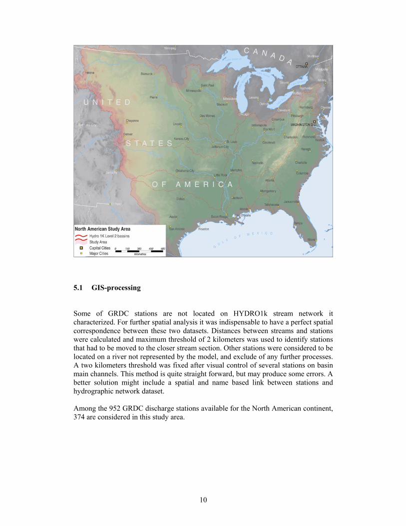
1988). Then, an iterative process was applied using SRTM DEM (USGS EDC) and these bisectors to progressively raise the level of water at these outlet points, calculate wetted perimeter and flow cross sectional area at each step, and solve Manning’s equation. Obtained level of water was then interpolated along stream network between each outlet station. This interpolation was processed for each stream section going from level one Strahler classification to the downstream lower point. Maximum of outputs was attributed to each stream cell. Flooded area was obtained by filling SRTM DEM using interpolated water level values. 4.3 Calibration An approach for model calibration was tested using GRDC stations located on Missouri and Mississippi rivers. Above described GIS process was applied with station 1993 maximum discharge values and different Manning roughness coefficient. After comparison with Dartmouth Flood Observatory 1993-dataset of flooded area, roughness coefficient of 0.05 was selected, which correspond to a winding stream with weeds and pools (Applied Hydrology, Chow, Maidment and Mays, 1988). 5 First test zone: North America As explained above the regression method described here has only been used at a local level, for example for states of USA. In the study of South-Dakota streams, groups have been made according to the particular geography of the state with very careful attention to some particular cases and back and forth between classification and regressions. Such a study is not possible by a single team at the global scale for several reasons, and not possible at all for the moment for problems of data. Our idea is to try regressions at the global scale -and hence we will have less precise results. In particular, the choice of groups cannot be based on a very precise geographic study of each particular place and will be done on the only available global data. It has then been decided to chose at first a test-zone where data are expected to be reliable and with an important geographical density of gauging stations. So was chosen the whole North America for testing the regression method. This choice would also enable to do some comparisons with existing local studies. For reasons of schedule, the final peak-flow estimation was not possible on the whole zone because it would have need the GIS-processing for all level 4 basins. It was decided to estimate the peak-flows only for ungauged stations of Missouri and Mississippi level 2 basins, which are represented on the following map, the whole North America estimates being only a question of GIS-processing time.

10

5.1 GIS-processing Some of GRDC stations are not located on HYDRO1k stream network it characterized. For further spatial analysis it was indispensable to have a perfect spatial correspondence between these two datasets. Distances between streams and stations were calculated and maximum threshold of 2 kilometers was used to identify stations that had to be moved to the closer stream section. Other stations were considered to be located on a river not represented by the model, and exclude of any further processes. A two kilometers threshold was fixed after visual control of several stations on basin main channels. This method is quite straight forward, but may produce some errors. A better solution might include a spatial and name based link between stations and hydrographic network dataset. Among the 952 GRDC discharge stations available for the North American continent, 374 are considered in this study area.

11

5.2 Composition of groups. Given the set of basin and climatic variables -for gauging stations of the whole North America- provided by the GIS-processing above, the peak-flow estimates are then computed using Pearson type III law, as explained before. Next step is to constitute some groups. Remark that in the general case, groups are not supposed to be geographically constrained, as two sites with close values on variables else that XCOORD and YCOORD can be geographically very far. From a certain point of view, it is an advantage of the method. However, the example taken here staying in North America, this type of consideration is less relevant and we would let enter those coordinates in consideration for the formation of groups. At first, a Principal Components Analysis (PCA) was made based on the set of numeric (transformed) variables. Looking at the circle of correlation, one can see that first component is explained by the variables LDAREA, LMCHLENGTH and LKGRAV and can be interpreted as “size” and second one is explained by variables LMEANALT, LMNSLOP and LCHSLOP and can be interpreted as “elevation”. But the scree-plot is regularly decreasing and score plots in principal planes show no groups. Other tries had been performed on smaller subset of variables, without certain variables such LDRAREA which have a great probability to be in the regression formula itself, but with no more success. As peak-flows records depend clearly on meteorology, the second try is to make groups according to the variable CLIMAT. That variable takes theoretically 38 values and groups would be here too small to perform any reasonable regression. For this reason, a first classification was made following the great classes: Polar and Subpolar (1-5), Boreal (6-10), Cool temperate (11-16), Warm temperate (17-23), Subtropical (24-30) and Tropical (31-38). A lot of regressions were performed on the different groups, which were significant but the two bigger groups (Boreal and Cool temperate) were showing the less good results. It has then been decided to split each of both in two subgroups, which gives the final climate classification:

Class CLIMAT Description 1 1 to 5 Polar and Subpolar 2 6 to 8 Boreal (desert to moist forest) 3 9 to 10 Boreal (wet and rain forest) 4 11 to 13 Cool temperate (desert and steppe) 5 14 to 16 Cool temperate (moist to rain forest) 6 17 to 23 Warm temperate 7 24 to 38 Subtropical and Tropical

Once again the study of several regressions showed that certain groups are inhomogeneous, especially group 3, and a descriptive study was performed on the variables for that particular group, which appear to split into two subgroups according to the elevation LMEANALT. This leads to elaborate the following general strategy, which could be applied in global cases. 1. Construct groups of reasonable size according to values of variable CLIMAT

12

2. See if any variable or small number of variables splits the group As explained before, we allow us in this particular example of North America to use the geographic coordinates XCOORD and YCOORD. As seen before, the variable LMNSLOPE was bimodal on the whole set and is interesting to observe in the groups; As other variables were not significantly splitting any groups, the research of subgroups has been focused on the study of those four variables, individually, by sets of two (matrix plots) and four at the time by use of PCA. It gave the following results: On class 1, the PCA of the four variables showed 2 or 3 subgroups and a cluster analysis showed there was only two subgroups, and hence constructed those two subgroups. On class 2, analysis showed no subgroups. On class 3, cluster analysis enabled to construct the two subgroups discovered above. On class 4, no subgroups. On class 5, two subgroups. On class 6, no subgroups; On class 7, splitting was leading to construct a too small subgroup on which no regression could be performed, so it was decided not to split it. This study has established the final classification in ten groups: 1.1, 1.2, 2, 3.1, 3.2, 4, 5.1, 5.2, 6, 7 5.3 Regression formulae. Following the work of S.K.SANDO on South Dakota streams, next step is to elaborate a regression formula on each of those ten groups. It is explained in his paper that the best regression method would be the General Least Square (GLS) regression because of the different variances of different sites and the non–independence of records between different sites. The GLS method takes into account this covariance structure to have better regression results. Unfortunately, there was no time left to test that method which requires use of specific software, as GLS in all its generality (needed here) is not implemented in usual statistical software. However, the residual analysis in the further ordinary regressions will show no structure and frequently a normal distribution, which let think that the results with the two methods could be not so different. Furthermore, in that study on South Dakota, the choice of variables in the regression formula was done with ordinary regressions (because there’s a lot of regressions to be done before making his mind) so it can reasonably be estimated that regression formulae appearing below are not so different than with GLS method. For each group, a best subset regression was first performed to have a general picture. Then, combining contradictory arguments such as better R-square and significativity of variables, with help of Mallow’s Cp and a systematic analysis of residuals, searching for a very small number of variables in the case of small groups (and a limited number of variables for the others), adding or subtracting variables one by one of the model, it has been selected a “best” regression formula. Variables involved in those formulae, as well as their p-values, standard deviations of residuals, R-square, adjusted R-square and size of groups, are given in the following table. For certain groups, one or more outliers have been taken apart for establishing regression formula. For all groups but one, residual analysis was satisfactory. All the details on outliers and regressions are given in appendix. Remark that the study of the second test-zone and cross-validations between the two test-zones described in the next section have shown that even variables which seem

13

statistically very significant (very low p-value) can be irrelevant from the physical point of view. This observation led us to reconsider the study of regressions for group 1.1 and group 3.1 in order to keep a smaller number of variables. Results given here are the definitive ones –different from those of intermediate report. Group 1.1 1.2 2 3.1 3.2 4 5.1 5.2 6 7 N 52 16 83 13 23 40 9 50 24 28 constant -0.418 6.04 2.59 -0.250 -0.891 4.87 -5.45 -0.536 -8.36 -1.60 (p-value) (0.075) (0.006) (0.007) (0.749) (0.066) (0.014) (0.026) (0.012) (0.000) (0.085)LDRAREA 0.819 0.582 0.673 0.806 0.875 0.663 1.00 0.786 0.872 0.380 (p-value) (0.000) (0.000) (0.000) (0.001) (0.000) (0.000) (0.001) (0.000) (0.000) (0.000)LPRMEAN 1.53 2.55 1.00 (p-value) (0.016) (0.000) (0.000)LMEANALT -1.40 -2.18 (p-value) (0.000) (0.003) LMNSLOPE 1.15 1.21 0.271 (p-value) (0.000) (0.001) (0.000) LTFORCOV 0.411 (p-value) (0.008) LDRFREQ 1.63 (p-value) (0.018) S 0.194 0.171 0.373 0.273 0.184 0.414 0.157 0.173 0.364 0.209 R^2 82.7% 71.3% 71.1% 66.2% 79.9% 63.7% 85.4% 86.0% 77.6% 52.9% R^2-adj 82.4% 66.9% 70.0% 63.1% 77.9% 60.7% 80.6% 85.4% 75.5% 49.1% No surprise that the variable LDRAREA is always the more significant, as AREA is intuitively the most important factor and as it was also the case in the South Dakota study. No surprise also that its coefficient is less than 1 because recurrence interval peak-flow must have a sub-additive behaviour: if a basin is a disjoint union of two sub-basins, hundred years-recurrence peak-flow of the sub-basins won’t generally occur at the same time and then the hundred years-recurrence peak-flow of the total basin is less than the sum of the sub-basins’ peak-flows. It is also conform to intuition that the precipitation has a positive influence on the peak-flow magnitude, and the same for the mean slope of the basin or the density of hydrographic network. For the mean elevation, negative effect could be interpreted by the link with other variables because low elevation basins and high elevation basins have usually very different characteristics. There is also probably a subtler link to explore between the mean elevation and the slope because the two variables LMEANALT and LMNSLOP occur very frequently simultaneously in the regressions. The effect of the forest cover is not evident but could be explained by the fact that it occurs for Boreal climate for which the forest cover can be correlated with the rain precipitation. Geographic randomness of residuals has been checked on a global map of residuals given in appendix. 5.4 Peak-flow values for ungauged sites. These regression formulae enable the estimation of hundred years peak-flow estimate for ungauged sites, provided each ungauged site is attributed to a group. This attribution is done by the way of climatic value and eventually by performing discriminant analysis in the case of two groups in one climate class. This discriminant

14

analysis also enables to check the splitting in groups. If to perform on a global scale, this discrimination has to be programmed to treat all automatically, unless the risk of error when manipulating data between the different groups is real. 5.5 Flooded area estimations A GIS process for Manning roughness coefficient calibration was applied on this region, as described in point 4.3. This approach is a first attempt and should be developed in further method extrapolations at a global scale. As Manning coefficient depend on channel surface, calibration process might be reiterate for specific stream section, and for different return period. Extended spatial datasets of flooded areas for specific events is indispensable in this calibration process. Nevertheless, some correspondences between distant but similar basins located in identical climatic zones might probably be established and use when footprints datasets are not available. 6 Second test zone: South America Considering the rather encouraging results of the first test, it has been decided to try the method on a zone involving developing countries and where density of gauging stations is less important, namely the whole South America. Such a test would give a good index for the feasibility at the global level. Moreover, it has been decided that the GIS-processing producing the basin and climatic variables would be run on the whole zone, which would enable an estimation of such a processing at the global level. This and a new statistical analysis would also enable the peak-flow estimates by the regression method on the whole zone. Unfortunately, there was no hope to perform the flooded area estimations on the whole zone before the deadline, for those estimations are delicate and time-consuming, and such estimations have been restricted to the zone shown on map below.

15

6.1 GIS-processing Due to larger distances between stream network and GRDC stations as compared to the one in the North American study area, a different process was used to allocate these stations to the right river section. According to Strahler classes, different distance thresholds were considered to link stations with stream section. NIMA Vmap0 river network dataset and river names included in GRDC station attribute file were considered in complementary name based link. 6.2 Composition of groups. Given the set of basins and climatic variables -for gauging stations of the whole South American continent -, the peak-flow estimates are computed as before. The general strategy developed for the first test-zone is then applied: 1. Construct groups of reasonable size according to values of variable CLIMAT 2. See if any variable or small number of variables splits the group The distribution of variable CLIMAT is of course very different than for North America and most of the gauging stations are in the categories Subtropical and

16

Tropical. Those two categories correspond to the group 7 of the North America study, which will be denoted here as group NA7. Concerning the other climatic categories, only 20 stations are ranging from Boreal to Warm temperate. A first attempt consisted in making 4 climatic classes: Polar, Subpolar and Boreal (1 to 10), Cool and Warm temperate (11 to 23), Subtropical (24 to 30) and Tropical (31 to 38). But first class was too small (4 stations) to enable regressions and different attempts showed that the adjunction of that first class to the second was surprisingly leading to no significant changes in the regressions results. It has then been decided to join the first and second classes and, rather to change all the classification, new class is denoted by 12. The three climatic classes are then:

Class CLIMAT Description 12 1 to 23 Polar to Warm temperate 3 24 to 30 Subtropical 4 31 to 38 Tropical

The descriptive analysis of other variables shows no particular splitting and it was then decided to take as definitive groups the three classes above. According to those variables, the set of stations is much more homogenous than the set of North America. Even some regressions on the whole set were tried which were providing some interesting results. Nevertheless, regressions by groups are more precise and for each group the most relevant formula was search. This has been done in parallel with several cross-validation studies between South and North America, which have given some information on the variables to take into account in the regressions. 6.3 Cross-validation between South and North America The first study concerns South American groups 3 (Subtropical) and 4 (Tropical), named SA3 and SA4, and North American group NA7 (Subtropical and Tropical). The union of groups SA3 and SA4 is denoted by SA34 and it is also considered subgroups of NA7 corresponding to Subtropical climate, denoted by NA71 and to Tropical climate, denoted by NA72. The idea is to compare groups SA34 and NA7, groups SA3 and NA71, and groups SA4 and NA72, which correspond to comparable values of the variable CLIMAT. This comparison is done by performing a regression on each group simultaneously and testing it on the other corresponding group. Considering group SA34, a preliminary study leads easily to consider the 2 sets of explanatory variables: LDRAREA and LPRMEAN (2 variables) and LDRAREA, LPRMEAN and LSOIL_HC (3 variables) and the two corresponding regressions are performed. For group NA7, it is taken the formula given by the North American study, involving LDRAREA and LPRMEAN. A regression is also performed on the total of the two groups SA34 and NA7, named group 347, using those two variables. For each station of group 347 are then computed 4 peak-flow estimates by the four regression formulae above (estDP34, estDPS34, estDP7 and estDP347) and computed the four corresponding residuals (resDP34, resDPS34, resDP7 and resDP347). The box-plot and statistics below depicts those residuals.

17

Variable Group N Mean StDev Median resDP34

7 34

28 90

-0.012 0

0.30 0.33

0.010 -0.006

resDPS34

7 34

28 90

-0.043 0

0.34 0.31

0.062 -0.017

resDP7

7 34

28 90

0 0.066

0.20 0.40

-0.007 0.052

resDP347

7 34

28 90

-0.009 0.003

0.26 0.33

-0.011 0.015

(As can be verified in the table above, for a given group, the residuals are smaller and of zero mean for the regression formulae constructed with that group -e.g. resDP7 for group NA7-, which is a consequence of mathematical definition of regression.) Three important remarks can be derived from those values and box-plots. Firstly, the residuals for a group corresponding to a regression from the other group have relatively good standard deviation, considering the fact that the groups are geographically very far. For comparison, the values 0.30 or 0.40 are less than certain residual standard deviations within groups of North America. It is relatively surprising due to the fact that the classification is very coarse: it depends only on a set of values of the variable CLIMAT and for example the variable CLDERMONTH takes very different values on groups NA71 and SA3 (Subtropical). Relatively surprising also the fact that there is no significant bias as can be seen on the means and medians.

18

Secondly, considering estimations DP34 and DPS34, we see that introduction of the variable LSOIL_HC in the regression, beside giving of course a slightly better estimate for group SA34, gives a worse estimation for group NA7. Unless it can be explained by geophysical differences between North and South America, it could be interpreted as over-fitting. In others words, there is a difference between statistic significance and physical significance. In order to use regression formulae for extrapolation, it is essential to have a physical significance of variables and one should be extremely careful in the choice of those variables. It is better to keep very few variables for which physical significance is certain. For that reason, variable LSOIL_HC has been taken apart. Certain regressions of the first test-zone have also been revised as was mentioned in the corresponding section. Thirdly, the total regression DP347 gives results very close from those of regression DP34 on group SA34 and is better on group NA7: in that case, the regression on the big group 347 gives very good results and that could be an indication to chose not too small groups, though sufficiently homogeneous. It has been then studied cross-validations considering Subtropical and Tropical classes SA3, SA4, NA71 and NA72. For group SA3, it has been proceed to a regression using variables LDRAREA and LPRMEAN, called DP3. For group SA4, variable LPRMEAN wasn’t statistically significant so it has been done a simple regression with variable LDRAREA, called D4. It has then been computed estimations for group 347 corresponding to the five regressions DP34, DP7, DP347, DP3 and D4. Corresponding residuals are shown on the following box-plot and table.

19

Variable Group N Mean StDev Median resDP34 3

4 71 72

75 15 21 7

0.008 -0.040 0.005 -0.061

0.34 0.30 0.27 0.39

0.005 -0.021 0.004 0.037

resDP7 3 4 71 72

75 15 21 7

0.067 0.062 -0.005 0.015

0.41 0.40 0.20 0.21

0.056 -0.055 -0.009 0.103

resDP347 3 4 71 72

75 15 21 7

0.010 -0.033 0.011 -0.068

0.34 0.33 0.24 0.32

0.035 -0.019 -0.010 -0.012

resDP3 3 4 71 72

75 15 21 7

0 -0.052 0.017 -0.084

0.34 0.32 0.26 0.36

-0.010 -0.052 0.008 -0.038

resD4 3 4 71 72

75 15 21 7

0.042 0 -0.028 0.026

0.37 0.28 0.39 0.61

0.043 0.011 0.016 0.327

One can see on the box-plot and table that the group NA72 is badly estimated by the regression D4, though the two groups have the same values for the variable CLIMAT. This group has also a less good estimation by DP34 than by DP3 which consolidates the first fact. This could be another indication that the variable CLIMAT maybe doesn’t express what is commonly meaning by the word “climate” –for instance the question of temperature. For example the formula DP3 estimates much better group NA71 and in a certain sense, group NA72 (i.e. Tropical zone of North America) has more in common with group SA3 (i.e. Subtropical zone of South America) than with group SA4 (i.e. Tropical zone of South America). In a further study, it would be important to examine details of the construction of the variable CLIMAT used here. Concerning the group SA12, a regression using the two variables LDRAREA and LPRMEAN was chosen, denoted by DP12. An affectation of each station to a group of North America was also proceeded, according to the procedure used in the first test, and then peak-flow were estimated using the corresponding regression formulae. This has shown that the first choice of regression for group NA3.1 during the first test had probably too much variables (3) and this was modified as previously mentioned (only 1 variable). The new estimates for corresponding stations of South America were surprisingly good (residuals less than 0.1), though the number of stations is too small for statistical evidence. Other stations of group SA12 are rather well estimated by North American regression, except two stations corresponding to group NA4, what is probably explained by the fact that regression was not so good for group NA4 itself. 6.4 Test of the PLS regression The Partial Least Square (PLS) regression method was also tested. This on is very famous because it doesn’t require any choice of variables. The idea of PLS is to first find the linear combination of variables which has the best correlation with the response, and then to continue the process on residuals and so on, in order to obtain –as for PCA- a few orthogonal components with a high correlation with the response and then to perform a linear regression of the response versus these components. On the statistical software used here, PLS is implemented with an option of automatic

20

cross-validation of the components. On the group SA3, number of cross validated components was three, the standard deviation of the residuals was 0.30 and the standard deviation of the residuals obtained by “leave-one-out” cross-validation was 0.34. Those values seem comparable and even slightly better than those obtained by standard regression. It was then proceeded estimations for group NA71 with this PLS formula based on group SA3. Unfortunately, for those estimations, the residuals had a mean -0.6140 and standard deviation 0.2310 which shows an very large overestimation. The problem is probably that the weights of variables into components rely on no physical signification, which is in link with the conclusions of the above cross-validation. In conclusion, PLS regression seems not adapted to the problem studied here. 6.5 Final regressions According to the previous study, choice of regressions and corresponding data are summarized in the following table and details are in appendix.

Group 12 3 4 N 20 75 15 constant (p-value)

-5.42 (0.000)

- 3.38 (0.000)

-0.676 (0.273)

LDRAREA (p-value)

0.808 (0.000)

0.788 (0.000)

0.881 (0.000)

LPRMEAN (p-value)

1.73 (0.000)

1.01 (0.000)

s 0.32 0.34 0.29 R^2 78.2% 67.5% 78.5% R^2-adj 75.7% 66.6% 76.9%

Geographic randomness of residuals has been checked on a global map of residuals given in appendix. Peak-flow estimates for ungauged stations are then performed using the regression formula corresponding to the climatic group of each basin. 6.6 Flooded area estimations As level 4 basins are not available in some regions, like in the Amazonian basin region, and to restrain time consuming processes, a region located to the North of Buenos Aires and corresponding to seven level 2 basins were selected for flooded area estimation. Furthermore, Dartmouth Flood Observatory has good datasets for this region. Model calibration realized for North America was not achieved for this region and a identical 0.05 Manning coefficient was used. But same process may be applied in order to identify regional particularities.

21

7 Remarks and recommendations for further studies 7.1 Data.

7.1.1 SRTM and HYDRO1k. Use of SRTM (90 m) instead of HYDRO1k DEM (1 km) should be considered in further development. Time-consuming global GIS process as a consequence of SRTM high resolution has to be evaluated. Furthermore, one should consider that any DEM used for streams and floods modeling must be hydrologically correct. Nevertheless, the approach applied in this study, which is using HYDRO1k DEM for saving time during basin variable production, and then use estimated peak flow values to fill SRTM DEM seems to be interesting and might be developed in further studies.

7.1.2 Climatic variables. One important climatic variable that should be taken in account in further analysis is the Precipitation Intensity Index. This index represents twenty-four hours precipitation intensity in millimeters, with a two years recurrence interval. Calculation of such an index might be achieved at a global scale using NCEP/NCAR Reanalysis daily time-series.

7.1.3 Soil characteristics. Soil Infiltration Index described by Natural Resources Conservation Service and used for similar U.S. national studies might be used instead of hydraulic conductivity. 7.2 GIS-processing

7.2.1 GRDC stations spatial selection. Method for selection of discharge stations as describe above (2.1) was adopted to use HYRDO1k level 4 basin outlets as a spatial reference. Other spatial selection methods might be considered which might retain larger sample of discharge stations.

7.2.2 Main channel. Delineation of basin main channel is based on HYDRO1k flow accumulation grid on which a minimum threshold of 400 was applied. In order to improve relevance of this parameter and the derived variables, it might be recommended to use specific threshold for each climatic zones or a vector dataset like NIMA Vmap0 hydrographic network.

7.2.3 Manning’s equation and discharge vs. stage rating curves. Manning’s equation might be used for flooded area estimation, but roughness coefficient has to be fixed in a relevant way. Local estimation of this parameter has probably to be achieved in order to obtain flooded area relevant estimation.

22

Discharge vs. stage rating curves might be also used, if available, for flooded area estimation. 7.3 Statistical analysis

7.3.1 Composition of groups The composition of groups remains a subtle problem and other methods could be imagined. In a further study, it would be important to examine details on the construction of the variable CLIMAT used here and eventually to try other Datasets. After determining the groups, it would be important to get a totally automated allocation of ungauged stations to groups.

7.3.2 Regressions As seen in the study on South Dakota, it would be more relevant to use GLS regressions -by the way of a software like GLSNET or by home-made programming. Also out-of-sample regressions could be performed to give estimations of prediction errors. But the more important seems to chose few and physically significant variables for regressions. Human interpretation remains a crucial point, and it has also been seen that the PLS regressions were not adapted to our problem, even using automated cross-validations.

7.3.3 Validations Another important and interesting part of a further study would be to compare estimations and regressions formulae to those obtained locally by other teams. Also each new zone studied would lead to new possibilities of cross-validations and would give a new point of view on groups’ construction. 8 Conclusion The method described and tested in this study seems to provide good chances to be extrapolated to the global level. However, regional particularities would have to be considered during each method steps, and such study would probably mobilize several persons during several months. The obtained results might probably be of different precision due to the variability in both density and quality of data, as well as in the particularities inherent to specific regions. Quality of global datasets should be analysed for each regional studied area. The more the number of gauging stations (with regular inputs), the more the treatment could be refined.

23

9 Appendixes Appendix A References Chow, V. T., Maidment, D. R., Mays, L. W., 1988, Applied Hydrology. Musy, A., Soutter, M., 1991, Physique du sol. Bravard, J.-P., Petit, F., 2000, Les cours d’eau, Dynamique du système fluvial. Musy, A., 2005, Hydrologie générale. http://hydram.epfl.ch/e-drologie/. K.L. Verdin, J.P. Verdin, 1999, A topological system for delineation and codification of Earth’s river basins. United States Water Resources Council’s Hydrology Subcommittee, 1982, Bulletin 17B: Guidelines for determining flood flow frequency. Sando, S. K., Water-Resources Investigation Report 98-4055: Techniques for Estimating Peak-Flow Magnitude and Frequency Relations for South Dakota Streams.

24

Appendix B Details on peak-flow regressions Reference numbers are relative to HYDRO1k database. North America Best regression for group 1.1 This regression has been revised due to the experience of cross-validations during the study of second test zone (South America). One station without hydrologic values (4695). One station taken apart because of uncertainty of data (2643). It has been also taken apart the station 1926 because of his very atypical characteristics, such as conjunction of low MEANALT and large MNSLOPE. It would be relevant in a further study to examine separately such atypical basins for prediction. It has then been taken only one variable because the difference between one or more variable in the part of variance explained by regression was very small and it has been seen in the cross-validation with South America that only very few variables are physically significant. Residual analysis is very good. The regression equation is logQ100 = - 0.418 + 0.819 LDRAREA N = 52 Predictor Coef SE Coef T P Constant -0.4180 0.2297 -1.82 0.075LDRAREA 0.81929 0.05296 15.47 0.000 S = 0.193501 R-Sq = 82.7% R-Sq(adj) = 82.4% Analysis of Variance Source DF SS MS F P Regression 1 8.9600 8.9600 239.30 0.000Resid. Error 50 1.8721 0.0374 Total 51 10.8322 Best regression for group 1.2 Chosen near minimal Mallow's Cp, preferring variable LDRAREA instead of LMCHLENGTH because the first is constantly appearing as main factor elsewhere and the two are very strongly correlated. Good residual analysis The regression equation is logQ100 = 6.04 + 0.582 LDRAREA + 1.63 LDRFREQ

25

N = 16 Predictor Coef SE Coef T P Constant 6.041 1.834 3.29 0.006LDRAREA 0.5822 0.1048 5.55 0.000LDRFREQ 1.6274 0.5989 2.72 0.018 S = 0.171339 R-Sq = 71.3% R-Sq(adj) = 66.9% Analysis of Variance Source DF SS MS F P Regression 2 0.94742 0.47371 16.14 0.000Resid. Error 13 0.38164 0.02936 Total 15 1.32906 Source DF Seq SS LDRAREA 1 0.73068 LDRFREQ 1 0.21674 Best regression for group 2 Chosen by minimizing Mallow's Cp. Bad residual analysis: they are non normal due to large and small values in greater amount than normally. Anyway, there is no good choice here from this point of view of normality of residues. Consequently, numeric indicators are to be examined very carefully. As p-values are very small (order 10^-4 or less), the robustness of the method insures that chosen variables are significant. From the point of view of prediction, the shape of residuals histogram insures that for a given symmetric interval around 0, the proportion of residuals is bigger than for the normal law with same standard deviation. The value of s can then be kept for prediction error (as real prediction error is smaller). The regression equation is logQ100 = 2.59 + 0.673 LDRAREA - 1.40 LMEANALT + 1.15 LMNSLOP N = 83 Predictor Coef SE Coef T P Constant 2.5937 0.9440 2.75 0.007LDRAREA 0.67256 0.07797 8.63 0.000LMEANALT -1.3957 0.3243 -4.30 0.000LMNSLOP 1.1521 0.1633 7.05 0.000 S = 0.373111 R-Sq = 71.1% R-Sq(adj) = 70.0%

26

Analysis of Variance Source DF SS MS F P Regression 3 27.0905 9.0302 64.87 0.000Resid. Error 79 10.9977 0.1392 Total 82 38.0882 Source DF Seq SS LDRAREA 1 18.2245 LMEANALT 1 1.9372 LMNSLOP 1 6.9288 Best regression for group 3.1 This regression has been revised due to the experience of cross-validations during the study of second test-zone (South America). It has then been taken only one variable because it has been seen that only very few variables are physically significant and the size of group is very small. It has been kept the constant unless it was clearly not significant because other regressions show clearly (what is intuitively clear) that a constant term was needed. Residual analysis is very good. The regression equation is logQ100 = - 0.250 + 0.806 LDRAREA N = 13 Predictor Coef SE Coef T P Constant -0.2497 0.7594 -0.33 0.749LDRAREA 0.8062 0.1736 4.64 0.001 S = 0.272781 R-Sq = 66.2% R-Sq(adj) = 63.1% Analysis of Variance Source DF SS MS F P Regression 1 1.6041 1.6041 21.56 0.001Resid. Error 11 0.8185 0.0744 Total 12 2.4226 Best regression for group 3.2 Regression on the total set gives very bad results. On the matrix plot of all variables, it is clear that there is a good linear link between logQ100 and LDAREA except for 4 points very far from the "line" (5562, 5971, 5343, 6970). These points are also outliers for one or several explicative variables. They need to be examined separately very carefully and cannot be taken into account in the regression estimation. Regression gives then some interesting results. The best regression cannot be chosen here by minimizing exactly Mallow's Cp because of the small amount of data versus the big number of variables. Nevertheless, a set of two variables has a Cp very close

27

to the minimum. In addition residual analysis is OK. It has been kept the constant unless it was not clearly significant because other regressions show clearly (what is intuitively clear) that a constant term was needed. The regression equation is logQ100 = - 0.891 + 0.875 LDRAREA + 0.411 LTFORCOV N = 23 Predictor Coef SE Coef T P Constant -0.8907 0.4585 -1.94 0.066LDRAREA 0.87478 0.09839 8.89 0.000LTFORCOV 0.4107 0.1394 2.95 0.008 S = 0.183757 R-Sq = 79.9% R-Sq(adj) = 77.9% Analysis of Variance Source DF SS MS F P Regression 2 2.6799 1.3399 39.68 0.000Resid. Error 20 0.6753 0.0338 Total 22 3.3552 Source DF Seq SS LDRAREA 1 2.3866 LTFORCOV 1 0.2932 Best regression for group 4 It has been taken apart a station (4644) which was an outlier for several variables, in particular LDAREA. Minimal Cp was obtained for 6 variables, which was too much for the number of stations. Nevertheless, as set of three variables has a low Cp and gives very good significance of variables and behaviour of residuals. The regression equation is logQ100 = 4.87 + 0.663 LDRAREA - 2.18 LMEANALT + 1.21 LMNSLOP N = 40 Predictor Coef SE Coef T P Constant 4.865 1.878 2.59 0.014LDRAREA 0.6635 0.1098 6.04 0.000LMEANALT -2.1783 0.6829 -3.19 0.003LMNSLOP 1.2098 0.3453 3.50 0.001 S = 0.413516 R-Sq = 63.7% R-Sq(adj) = 60.7%

28

Analysis of Variance Source DF SS MS F P Regression 3 10.7940 3.5980 21.04 0.000Resid. Error 36 6.1558 0.1710 Total 39 16.9499 Source DF Seq SS LDRAREA 1 8.6903 LMEANALT 1 0.0051 LMNSLOP 1 2.0986 Best regression for group 5.1 It is chosen a maximum number of two explicative variables because of the small size of the group. The best 2-set was the following, for which analysis of residuals is OK. The regression equation is logQ100 = - 5.45 + 1.00 LDRAREA + 1.53 LPRMEAN N = 9 Predictor Coef SE Coef T P Constant -5.452 1.864 -2.92 0.026LDRAREA 1.0017 0.1690 5.93 0.001LPRMEAN 1.5267 0.4601 3.32 0.016 S = 0.156886 R-Sq = 85.4% R-Sq(adj) = 80.6% Analysis of Variance Source DF SS MS F P Regression 2 0.86634 0.43317 17.60 0.003Resid. Error 6 0.14768 0.02461 Total 8 1.01402 Source DF Seq SS LDRAREA 1 0.59531 LPRMEAN 1 0.27103 Best regression for group 5.2 Minimal Cp is obtained for 5 variables but keeping two of them, LDAREA and LMNSLOP, gives a very close result in terms of R-square and s. Furthermore, those variables are very significant and the residual analysis is correct. The regression equation is logQ100 = - 0.536 + 0.786 LDRAREA + 0.271 LMNSLOP

29

N = 50 Predictor Coef SE Coef T P Constant -0.5360 0.2057 -2.61 0.012LDRAREA 0.78618 0.04768 16.49 0.000LMNSLOP 0.27147 0.05981 4.54 0.000 S = 0.172611 R-Sq = 86.0% R-Sq(adj) = 85.4% Analysis of Variance Source DF SS MS F P Regression 2 8.6158 4.3079 144.59 0.000Resid. Error 47 1.4003 0.0298 Total 49 10.0162 Source DF Seq SS LDRAREA 1 8.0019 LMNSLOP 1 0.6139 Best regression for group 6 Minimal Cp is obtained for 6 variables, which is too much with respect to the number of stations. Keeping two of them, LDAREA and LPRMEAN, gives a very good result in terms of R-square and s. Furthermore, those variables are very significant, residuals can be supposed normal (but very close to non-normal) and show no structure. The regression equation is logQ100 = - 8.36 + 0.872 LDRAREA + 2.55 LPRMEAN N = 24 Predictor Coef SE Coef T P Constant -8.359 1.404 -5.95 0.000LDRAREA 0.8717 0.1327 6.57 0.000LPRMEAN 2.5463 0.4154 6.13 0.000 S = 0.363706 R-Sq = 77.6% R-Sq(adj) = 75.5% Analysis of Variance Source DF SS MS F P Regression 2 9.6341 4.8170 36.42 0.000Resid. Error 21 2.7779 0.1323 Total 23 12.4120

30

Source DF Seq SS LDRAREA 1 4.6648 LPRMEAN 1 4.9693 Best regression for group 7 The minimal Cp is obtained for 4 variables LDRAREA, LPRMEAN, LMEANALT and CLDERMONTH, but the last one isn't significant and after removal, LMEANALT isn't significant too. The regression on the two last variables is the following. Residual analysis is good. The regression equation is logQ100 = - 1.60 + 0.380 LDRAREA + 1.00 LPRMEAN N = 28 Predictor Coef SE Coef T P Constant -1.6017 0.8933 -1.79 0.085LDRAREA 0.38034 0.09273 4.10 0.000LPRMEAN 1.0038 0.2079 4.83 0.000 S = 0.209044 R-Sq = 52.9% R-Sq(adj) = 49.1% Analysis of Variance Source DF SS MS F P Regression 2 1.22572 0.61286 14.02 0.000Resid. Error 25 1.09249 0.04370 Total 27 2.31821 Source DF Seq SS LDRAREA 1 0.20696 LPRMEAN 1 1.01877 South America Regressions have been chosen here according to the discussion presented in the text, i.e. by taking a few number of both statistically and physically significant variables. Best regression for group 12 It has been selected variables LDRAREA and LPRMEAN. Residual analysis is very good and the formula is the following. logQ100 = - 5.42 + 0.808 LDRAREA + 1.73 LPRMEAN N = 20

31

Predictor Coef SE Coef T P Constant -5.422 1.084 -5.00 0.000LDRAREA 0.8084 0.1450 5.57 0.000LPRMEAN 1.7253 0.2827 6.10 0.000 S = 0.315648 R-Sq = 78.2% R-Sq(adj) = 75.7% Source DF SS MS F P Regression 2 6.0905 3.0452 30.56 0.000Resid. Error 17 1.6938 0.0996 Total 19 7.7843 Source DF Seq SS LDRAREA 1 2.3801 LPRMEAN 1 3.7104 Best regression for group 3 It has been selected variables LDRAREA and LPRMEAN. Distribution of residuals is non-normal due to a few outliers. Consequently, numeric indicators are to be examined very carefully. As p-values are very small (order 10^-4 or less), the robustness of the method insures that chosen variables are significant. From the point of view of prediction, the shape of residuals histogram insures that for a given symmetric interval around 0, the proportion of residuals is bigger than for the normal law with same standard deviation. The value of s can then be kept for prediction error (as real prediction error is smaller). The regression equation is logQ100 = - 3.38 + 0.788 LDRAREA + 1.01 LPRMEAN N = 75 Predictor Coef SE Coef T P Constant -3.3772 0.8186 -4.13 0.000LDRAREA 0.78800 0.07094 11.11 0.000LPRMEAN 1.0100 0.2506 4.03 0.000 S = 0.340234 R-Sq = 67.5% R-Sq(adj) = 66.6% Analysis of Variance Source DF SS MS F P Regression 2 17.2919 8.6459 74.69 0.000Resid. Error 72 8.3347 0.1158 Total 74 25.6265

32

Source DF Seq SS LDRAREA 1 15.4112 LPRMEAN 1 1.8807 Best regression for group 4 It has been selected only variable LDRAREA. Residual analysis is good and the formula is the following. logQ100 = - 0.676 + 0.881 LDRAREA N = 15 Predictor Coef SE Coef T P Constant -0.6764 0.5913 -1.14 0.273LDRAREA 0.8813 0.1279 6.89 0.000 S = 0.290735 R-Sq = 78.5% R-Sq(adj) = 76.9% Analysis of Variance Source DF SS MS F P Regression 1 4.0135 4.0135 47.48 0.000Resid. Error 13 1.0988 0.0845 Total 14 5.1124

33

Appendix C Maps Hundred Year Return Period Peak Flow Magnitude for North American Studied Region

34

Hundred Year Return Period Peak Flow Magnitude for South American Continent

35

Geographical Randomness of Residuals for American Continent

36

Hundred Year Return Period Flooded Area for North American Studied Region

37

Hundred Year Return Period Flooded Area for South American Studied Region

Sources: Unites Nations Cartographic Section; NIMA Vmap0; ESRI Data & Maps 2003; USGS EDC Hydro1K; EU’s JRC GLC2000. For all maps, the boundaries and names shown and the designations used do not imply official endorsement or acceptance by the United Nations.