Global Income Distribution and Convergence 1800-2000 Peter Földvari (Warwick University) and Jan Luiten van Zanden (IISH/Utrecht University) 1. Introduction Recent research by a.o. Bourguignon and Morrison (2001) has shown that the long run trend in global inequality in the past 200 years is to a large extent dominated by inter-country differences in GDP per capita. In particular the strong increase in global inequality during the 19th and the first half of the 20th century is completely driven by the growing gap between the industrializing rich countries and the non-industrializing poor nations. In the second half of the 20th century this trend seems to have come to a halt, and the rise of global inequality appears to have slowed down markedly (and within country inequality is probably becoming more important). Again, the slowing down is driven by inter-country differences, in particular the increasingly strong performance of Asian economies (such as the Asian tigers and more recently India and China).

Explaining the development of inter-country differences in economic growth is therefore of fundamental importance for understanding the long term evolution of global inequality. The literature suggests two different approaches to this. One if the (neo)Marxian/dependencia view that inequality between (groups of ) countries is a structural feature of global capitalism; Wallerstein (1974), for example, traces the differentiation between the core and the periphery of the world economy back to the 16th century, and in essence argues that core and periphery are parts of the same system. This interpretation, which was quite popular in the 1970s, sees the growing disparities within the world economy during the 19th and first half of the 20th century as another expression of global capitalism, and therefore predicts that inequality will not decline strongly in the future.

The alternative approach that prevails in much of the literature about this topic is that these processes of divergence and convergence are driven by the gradual diffusion of the Industrial Revolution over the globe. Growing global inequality during the 1800-1950 period is dominated by the fact that the number of countries participating in ‘modern economic growth’ is only growing slowly. The Industria l Revolution began in Great Britain in the late 18th century, spread to North America and Western Europe during the first half of the 19th century, and since spread further to Eastern and Southern Europe, to Japan and the Asian Tigers, and most recently, to large parts of mainland Asia (see Dowrick and De Long 2003). This pattern of diffusion obviously has a strong spatial element – industrialization seems to move from country to country – but was also based on the ability of countries to develop the right institutions for industrialization (as the success story of Japan illustrates).

In this paper we try to elaborate and test this diffusionist interpretation of the development of global inequality. Our starting point is a paper by Robert Lucas (2000), in which he presents a simplified model of this diffusion process, which he uses to simulate the development of global inequality. He firstly assumes that the leading economy (Great Britain) is growing at a constant rate of economic growth (of 2 per cent per capita). The other countries that are member of the convergence club, have a growth rate that is equal to this 2 percent plus a catch up factor that is proportional to the percentage income gap between itself and the leader. This will cause all members of the

convergence club to eventually converge to the level of the leader. The final element of the model is linked to the probability that country X will enter the convergence club at some point in time. Lucas ignored the spatial and institutional dimensions of this process and simply assumed that this probability was increasing slowly in time (from .1 to 3 percent), which generated a model that was more or less able to simulate the development of world inequality (this increase from .1 to 3 percent was in turn linked to the general increase in income levels following Tamura (1996)).

This simplified model is the starting point of our paper. We would like to establish if such a model of gradually diffusion of the process of industrialization is able to explain the long term development of world inequality (and global economic growth) in a more satisfactory way that the alternative view, which postulates the stability world inequality. Our main focus is on empirically testing the Lucas model, using the Maddison (2001) dataset about the growth of the world economy between 1820 and 2001. We concentrate on three predictions of the model:

- the share of countries or the share of the world population that is member of the convergence club (i.e. as rich as the leading economy or growing more rapidly that it) is increasing in the long term, and these shares shows a logistic curve approaching 100% in the long run;

- global inequality (between countries) increases until more than 50% of countries/world population is member of the convergence club; afterwards, inter-country global inequality will begin to decline (see the appendix for a proof of this);

- the growth rate of world GDP also will increase during the first phase of the diffusion process (because the leader is growing at a constant rate of 2% per annum, but increasing numbers of countries will join the convergence club and initially grow even faster than 2%), until again a certain point is reached – when the majority of countries has converged – that the growth of world GDP will start to decline again; in the extremely long run, when all countries have converged, the growth rate of GDP per capita of the world population will be 2% per annum, the same as that of the leading country.

In the simulation by Lucas (2000) the turning point in both world inequality and the growth rate of world GDP is reached between 1950 and 2000, when indeed more than 50% of the world population is member of the convergence club. An important assumptions of the Lucas model is that once countries have joined the convergence club they will continue to converge; there is no exit from the convergence club, whereas the neo-marxian interpretation will probably assume that – after some point – exit will equal entrance to the convergence club, creating the stabile degree of inequality they consider to be characteristic for global inequality.

We study long term patterns; being a member of not of the convergence club is related to the long-term performance of an economy (one cannot assess convergence or non-convergence of individual countries on the basis of the growth experience during short periods of time). As a result, the number of periods for which this can be studied is rather limited; following Maddison we distinguish the following periods for which we define and measure membership of this club: 1820-1870, 1870-1913, 1913-1950, 1950-1973 and 1973-2001 (1780-1820 is sometimes added to the analysis). This we then use to study entrance and exit: which factors determine the spread of ‘modern economic growth’ (i.e. the entrance of countries to the convergence club), and – a factor ignored

by Lucas – why do some countries leave the convergence club? Two kinds of factors seem to play a role here: spatial patterns (countries near other countries that grow rapidly will be stimulated to grow rapidly as well), and institutional factors (which institutions determine the joining or the leaving of the convergence club?). 2. Data and sources The main source of data is Maddison (2003). The dataset containing population and per capita GDP data (in 1990 Geary-Khamis International USD) is available on- line at http://www.ggdc.net/maddison/Historical_Statistics/horizontal- file.xls. Since the data had a lot of missing observations before 1870, and especially during the first decades of the 19th century, these had to be filled in by interpolation. For the interpolation of population we used a log- linear method, that is, it was assumed that the growth rate of population was even during the missing periods. The GDP per capita was linearly interpolated. The missing GDP data was calculated from the interpolated population and GDP per capita.

Countries where there was no initial data on the GDP and population in 1820 (developing countries, and predominantly in Africa) required a further assumption: here, in the absence of more information, we used the average of the continent to fill in the missing initial observation. A disadvantage of this approach is that some African countries may sometime seem to have experienced very high economic growth between 1820 and 1870, while in fact it is just the continental average that proved to be too low in their cases. Therefore, all developing countries are subject to the limitation that they cannot enter the convergence club before 1871.

For similar reason, we omitted three Middle Eastern countries, Kuwait, The United Arab Emirates, and Quatar. According to the Maddison dataset, in these countries the per capita GDP was between 16000 and 30000 USD (at 1990 prices) in 1950, while in the same time the region had an average of 1776 $ only. These outliers, and their erratic behavior significantly biased the calculations of average GDP, growth and variance.

We also made adjustments to the estimates for China, following the critical review of Maddison’s estimates by Holz (2006), who in our view convincingly shows that the adjustment Maddison made to the official estimates of the growth of GDP between 1978 and 1995 – by substracting 2.78% annually – is unfounded. We return to the official growth rates for this period (by adding again 2.78% annually). The result of this is that, whereas according to the Maddison estimates China between 1949 and 1978 is one of the most dynamic economies in the world – and part of the convergence club – the revised estimates show a much lower rate of growth between 1949 and 1978, and China in those years in not part of the convergence club. The decision to follow Holz therefore has important consequences for the results of this paper.

Summing up, the dataset contains annual data of GDP per capita and population of 139 countries representing almost 100% of world population and world GDP (the whole Maddison dataset covers 142 countries). 3. The dynamics of the convergence club Dowrick and De Long (2003) already carried out a classification of countries based on their place in the convergence club. Their definition of convergence club is, however, based on conventions rather than on objective factors. In their view, a country enters the

convergence club when it assimilates the institutions, technologies and productivity levels typical of North-western Europe. The main problem with such classification is that it is necessarily based on secondary literature (which covers not all of the countries of the world and may be subjective), and basically just put our European or North-American perception of development and being developed in writing: the more Western you look, the more developed we will think you are.

But this may not necessarily be advantageous. For example, the Dowrick-DeLong classification fixes the position of Western-Europe within the convergence club, even though, by applying an alternative classification system, one may find that most of Western Europe dropped out of the convergence club after 1973. Now either we put an emphasis on institutional system, or we face the reality that there are no reserved seats in the convergence club. As an alternative, we offer an alternative classification, based on economic indicators. One may argue with good reason that our approach also based on simplifications, but this was necessary to remain more or less objective. Criteria of the convergence club The period between 1820 and 2001 was divided into five sub-periods: 1820-1870, 1871-1913, 1914-1950, 1951-1973, and finally 1974-2001 (coinciding with the development phases of capitalism by Maddison, 1991). For each period, each country had to meet at least one of the following two requirements in order to be counted as member of the convergence club. 1. The requirement of growth demands that a country had to grow faster on average than the technological leader (the United Kingdom before until 1914, and the USA afterwards). 2. The requirement of high level of income requires that a country has at least 80% of the GDP per capita of the technological leader (in other words: it is already converged). The second condition allows the long-run per capita income within the convergence club differ by 20%, which is important as country-specific differences (institutional background, geographical factors, size) may cause the log-run per capita output to differ and therefore one should not expect a perfect convergence. We intervened in the classification twice: First, as mentioned and reasoned in Section 2, no developing country was allowed to be member of the convergence club before 1871. Secondly, if a country was a member of the convergence club both in the periods 1870-1914 and 1951-1973, it was automatically counted as member between 1914 and 1950, as well. We consider membership of the convergence club to be a long-term feature of an economy, which is not affected by exogenous shocks as occurred during the 1914-1945 period. This also means that our estimates of membership of the convergence club after 1973 are preliminary, and only the future can tell if North-Western Europe (countries such as France, Germany, Belgium, The Netherlands and Sweden), whose performance during the post 1973 period does not allow us to include them in the convergence club, will only temporarily underperform or permanently leave the club. The same applies to the (formerly) planned economies of Eastern Europe and the (former) USSR, which also leave the club in the post 1973 period, but may re-enter or perhaps, with the benefit of hindsight, never ‘really’ have left it. Membership of the convergence club in the post 1973 is therefore a lower bound estimate.

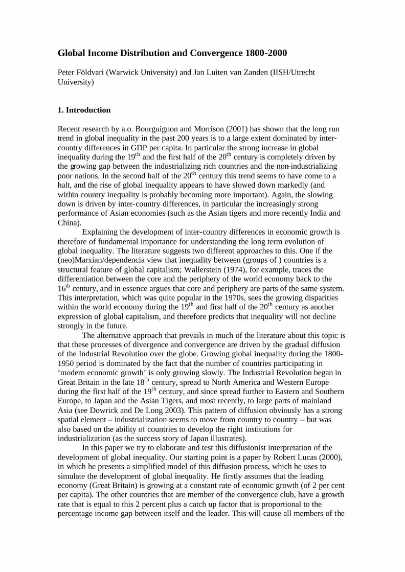
Changes in the convergence club The results from the classification based on the above-mentioned criteria is summarized in Table 1

Table 1 Entries to and departures from the convergence club

Period Entries to the club Departures from the club 1820-1870 Belgium, the Netherlands, Switzerland, the UK, Ireland,

Australia, New Zealand, Canada, USA None

1871-1913 Austria, Denmark, Finland, France, Germany, Italy, Norway, Sweden, Greece, Spain, Albania, Bulgaria, ex-

Czechoslovakia, Hungary, Poland, Romania, ex-Yugoslavia, ex-USSR, Argentina, Chile, Mexico,

Uruguay, Venezuela, Trinidad and Tobago, Japan, Hong Kong, Singapore, Sri Lanka, Israel, Lebanon, Syria, Palestine, Algeria, Gabon, Ghana, Mauritius,

Namibia, Reunion, Seychelles, South Africa

None

1914-1950 Brazil, Peru, Jamaica, Morocco Argentina, Chile, Uruguay, Lebanon, Ghana, Mauritius, Namibia, Seychelles, South Africa

1951-1973 Portugal, Costa Rica, Dominican Republic, Costa Rica, Nicaragua, Panama, Puerto Rico, Indonesia, Philippines,

South Korea, Thailand, Taiwan, Malaysia, Mongolia, North Korea, Bahrain, Iran, Iraq, Oman, Saudi Arabia,

Turkey, Yemen, Angola, Botswana, Côte d'Ivoire, Guinea Bissau, Lesotho, Malawi, Mauritania, Nigeria,

Swaziland, Togo, Tunisia, Zimbabwe, Equatorial Guinea, Libya, São Tomé and Principe

New Zealand, Venezuela, Sri Lanka, Morocco

1974-2001 Chile, China, India, Burma, Pakistan, Sri Lanka, Vietnam, Cape Verde, Egypt, Mauritius, Seychelles

Belgium, France, Germany, the Netherlands, Sweden, Australia, Albania, Bulgaria, ex-Czechoslovakia,

Hungary, Poland, Romania, ex-Yugoslavia, ex-USSR, Brazil, Mexico, Peru, Costa Rica, Ecuador, Jamaica,

Nicaragua, Panama, Trinidad and Tobago, Philippines, Mongolia, North Korea, Bahrain, Iran, Iraq, Israel, Saudi

Arabia, Syria, Turkey, Yemen, Algeria, Angola, Côte d'Ivoire, Gabon, Guinea Bissau, Malawi, Mauritania,

Nigeria, Reunion, Swaziland, Togo, Zimbabwe, Libya, São Tomé and Principe

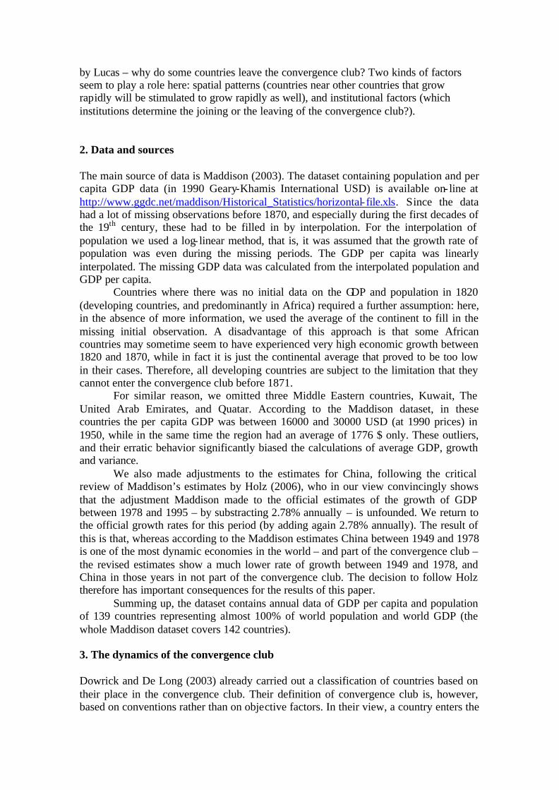
As Table 1 indicates, the membership to the convergence club changed quite a lot during the last two centuries. As it is found by other studies, the periods 1871-1913 and 1951-1973 were especially favourable for the world convergence, while the period 1974-2001 was almost catastrophic: countries that had been members of the club since 1820 or 1871, such as Belgium, France, Germany, the Netherlands, Australia, and Sweden lose their position. The reason is that their average growth rates remained below that of the USA long enough to lag behind in terms of per capita income by more than 20%.1 Obviously, as we argued in the introduction of this section, there is no guarantee that one remains in the club (the only exceptions are the UK before and the USA after 1914). Figure 1 reports the number of countries in- and outside the convergence club. It should be noted that the only period when the number of convergence countries exceeds the

1 The story of Western Europe exiting the convergence club after 1973 is rather complicated though, and we have not found a good solution for it; until the mid 1990s slow growth was linked to a slow increase (or even decrease) of labour input per capita, possible as a result of a different choice between leisure and income as in the US combined with increases in unemployment, early retirement etc. in Western Europe; in fact, labour productivity may have even increase faster there than in the US (Crafts 2004); since the mid 1990s however, productivity growth in the US has inrceased rapidly, mainly as a result of the ICT revolution, whereas Western Europe in general did not witness a similar growth spurt in productivity; so from the mid 1990s onwards there is a clear ’falling behind’; for that reasons we stuck to the results of working with the Maddison dataset; at some point in the future it will be possible though to study these two periods seperately: 1973-1995 and 1995-2020, and see how this changes our classification.

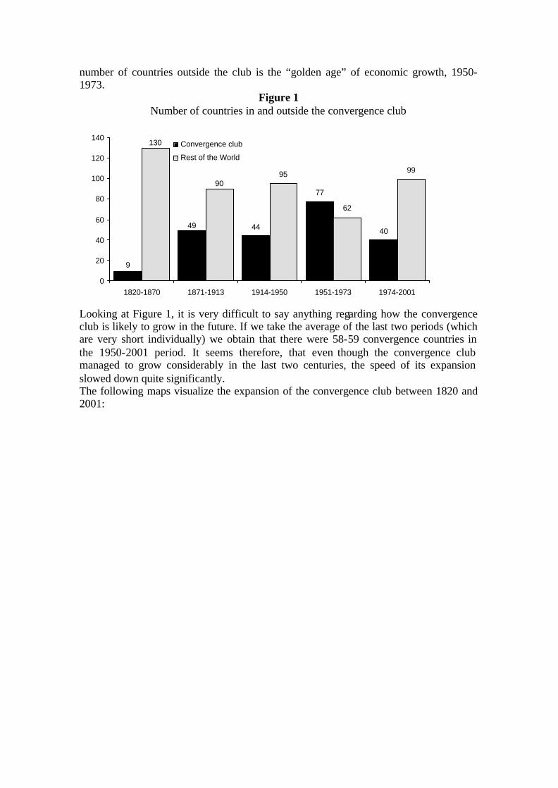
number of countries outside the club is the “golden age” of economic growth, 1950-1973.

Figure 1 Number of countries in and outside the convergence club

44

77

40

95

62

99

49

9

130

90

0

20

40

60

80

100

120

140

1820-1870 1871-1913 1914-1950 1951-1973 1974-2001

Convergence club

Rest of the World

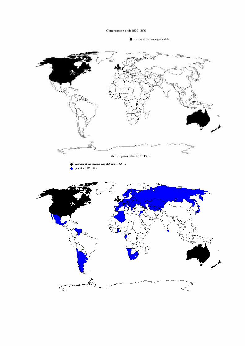
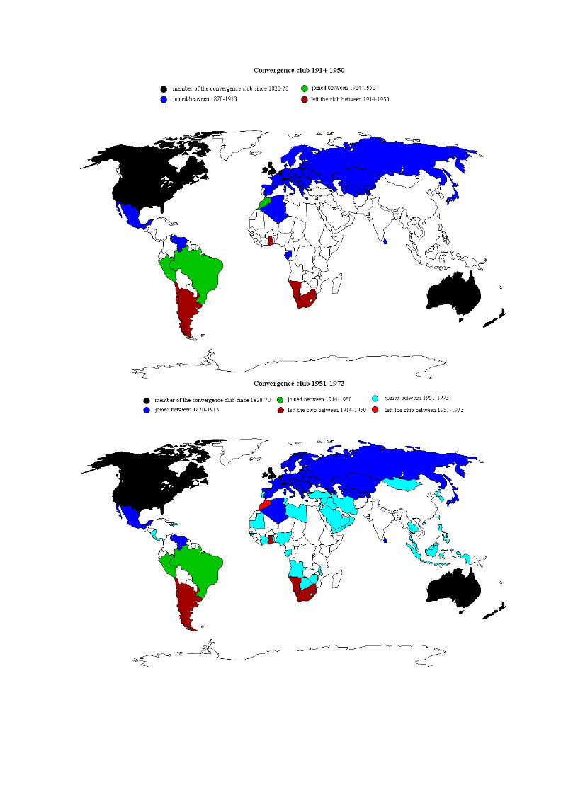
Looking at Figure 1, it is very difficult to say anything regarding how the convergence club is likely to grow in the future. If we take the average of the last two periods (which are very short individually) we obtain that there were 58-59 convergence countries in the 1950-2001 period. It seems therefore, that even though the convergence club managed to grow considerably in the last two centuries, the speed of its expansion slowed down quite significantly. The following maps visualize the expansion of the convergence club between 1820 and 2001:

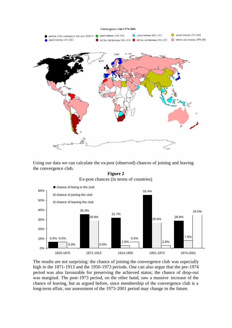
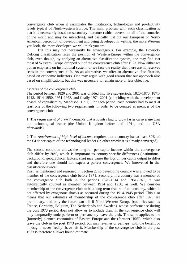
Using our data we can calculate the ex-post (observed) chances of joining and leaving the convergence club.

Figure 2 Ex-post chances (in terms of countries)

6.5%

35.3%31.7%

55.4%

28.8%28.8%

2.9%

26.6%

7.9%

0.0% 0.0%

6.5%2.9%

34.5%

6.5%

0%

10%

20%

30%

40%

50%

60%

1820-1870 1871-1913 1914-1950 1951-1973 1974-2001

chance of being in the club

chance of joining the club

chance of leaving the club

The results are not surprising: the chance of joining the convergence club was especially high in the 1871-1913 and the 1950-1973 periods. One can also argue that the pre-1974 period was also favourable for preserving the achieved status; the chance of drop-out was marginal. The post-1973 period, on the other hand, saw a massive increase of the chance of leaving, but as argued before, since membership of the convergence club is a long-term affair, our assessment of the 1973-2001 period may change in the future.

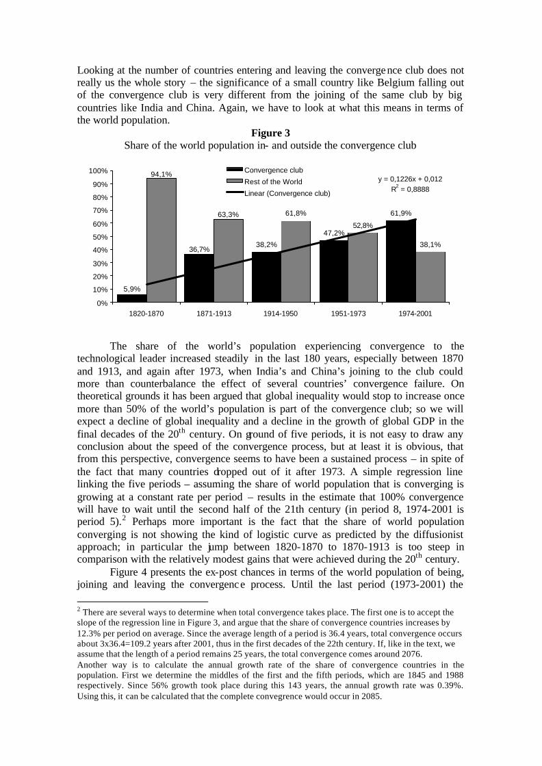
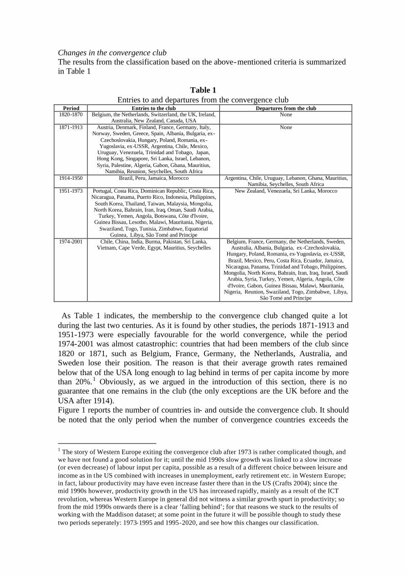
Looking at the number of countries entering and leaving the convergence club does not really us the whole story – the significance of a small country like Belgium falling out of the convergence club is very different from the joining of the same club by big countries like India and China. Again, we have to look at what this means in terms of the world population.

Figure 3 Share of the world population in- and outside the convergence club

38,2%

47,2%

61,9%61,8%

52,8%

38,1%36,7%

5,9%

94,1%

63,3%

y = 0,1226x + 0,012R2 = 0,8888

0%

10%

20%

30%

40%

50%

60%

70%

80%

90%

100%

1820-1870 1871-1913 1914-1950 1951-1973 1974-2001

Convergence club

Rest of the World

Linear (Convergence club)

The share of the world’s population experiencing convergence to the

technological leader increased steadily in the last 180 years, especially between 1870 and 1913, and again after 1973, when India’s and China’s joining to the club could more than counterbalance the effect of several countries’ convergence failure. On theoretical grounds it has been argued that global inequality would stop to increase once more than 50% of the world’s population is part of the convergence club; so we will expect a decline of global inequality and a decline in the growth of global GDP in the final decades of the 20th century. On ground of five periods, it is not easy to draw any conclusion about the speed of the convergence process, but at least it is obvious, that from this perspective, convergence seems to have been a sustained process – in spite of the fact that many countries dropped out of it after 1973. A simple regression line linking the five periods – assuming the share of world population that is converging is growing at a constant rate per period – results in the estimate that 100% convergence will have to wait until the second half of the 21th century (in period 8, 1974-2001 is period 5).2 Perhaps more important is the fact that the share of world population converging is not showing the kind of logistic curve as predicted by the diffusionist approach; in particular the jump between 1820-1870 to 1870-1913 is too steep in comparison with the relatively modest gains that were achieved during the 20th century.

Figure 4 presents the ex-post chances in terms of the world population of being, joining and leaving the convergence process. Until the last period (1973-2001) the 2 There are several ways to determine when total convergence takes place. The first one is to accept the slope of the regression line in Figure 3, and argue that the share of convergence countries increases by 12.3% per period on average. Since the average length of a period is 36.4 years, total convergence occurs about 3x36.4=109.2 years after 2001, thus in the first decades of the 22th century. If, like in the text, we assume that the length of a period remains 25 years, the total convergence comes around 2076. Another way is to calculate the annual growth rate of the share of convergence countries in the population. First we determine the middles of the first and the fifth periods, which are 1845 and 1988 respectively. Since 56% growth took place during this 143 years, the annual growth rate was 0.39%. Using this, it can be calculated that the complete convegrence would occur in 2085.

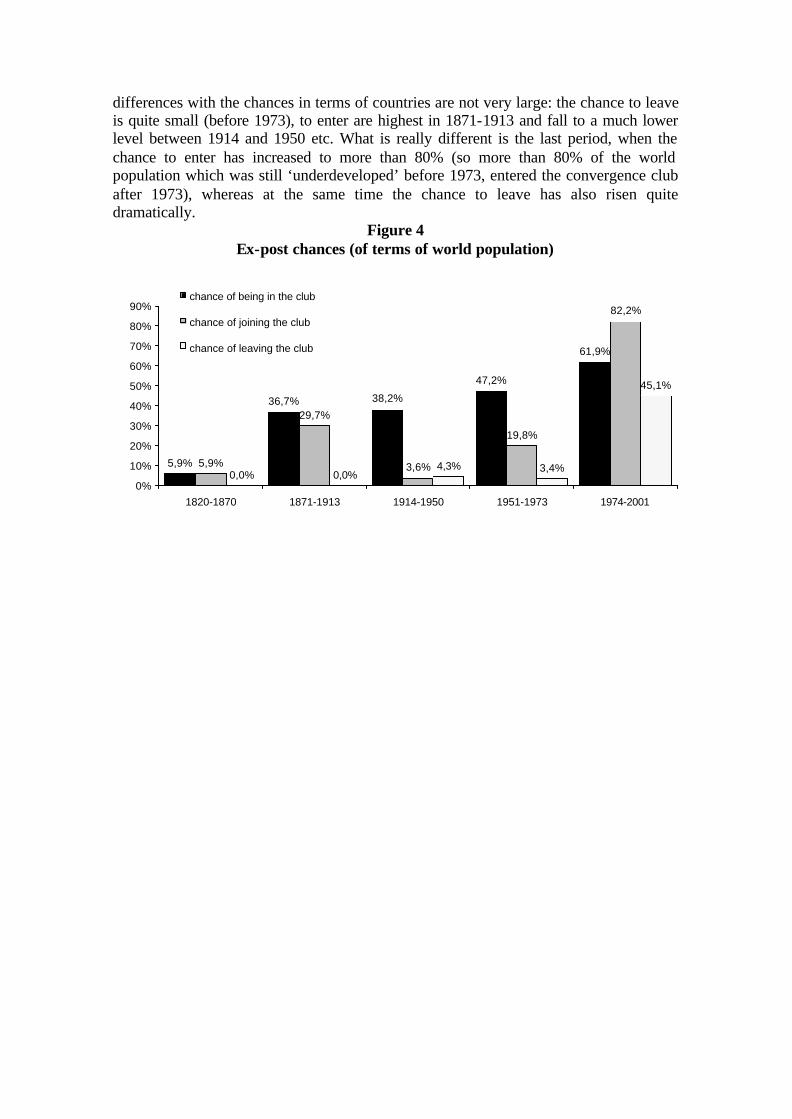
differences with the chances in terms of countries are not very large: the chance to leave is quite small (before 1973), to enter are highest in 1871-1913 and fall to a much lower level between 1914 and 1950 etc. What is really different is the last period, when the chance to enter has increased to more than 80% (so more than 80% of the world population which was still ‘underdeveloped’ before 1973, entered the convergence club after 1973), whereas at the same time the chance to leave has also risen quite dramatically.

Figure 4 Ex-post chances (of terms of world population)

5,9%

36,7% 38,2%

47,2%

61,9%

29,7%

3,6%

19,8%

82,2%

0,0% 0,0%4,3% 3,4%

45,1%

5,9%

0%

10%

20%

30%

40%

50%

60%

70%

80%

90%

1820-1870 1871-1913 1914-1950 1951-1973 1974-2001

chance of being in the club

chance of joining the club

chance of leaving the club

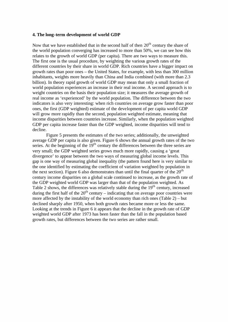
4. The long-term development of world GDP Now that we have established that in the second half of then 20th century the share of the world population converging has increased to more than 50%, we can see how this relates to the growth of world GDP (per capita). There are two ways to measure this. The first one is the usual procedure, by weighting the various growth rates of the different countries by their share in world GDP. Rich countries have a bigger impact on growth rates than poor ones – the United States, for example, with less than 300 million inhabitants, weights more heavily than China and India combined (with more than 2.3 billion). In theory rapid growth of world GDP may mean that only a small fraction of world population experiences an increase in their real income. A second approach is to weight countries on the basis their population size; it measures the average growth of real income as ‘experienced’ by the world population. The difference between the two indicators is also very interesting: when rich countries on average grow faster than poor ones, the first (GDP weighted) estimate of the development of per capita world GDP will grow more rapidly than the second, population weighted estimate, meaning that income disparities between countries increase. Similarly, when the population weighted GDP per capita increase faster than the GDP weighted, income disparities will tend to decline. Figure 5 presents the estimates of the two series; additionally, the unweighted average GDP per capita is also given. Figure 6 shows the annual growth rates of the two series. At the beginning of the 19th century the differences between the three series are very small; the GDP weighted series grows much more rapidly, causing a ‘great divergence’ to appear between the two ways of measuring global income levels. This gap is one way of measuring global inequality (the pattern found here is very similar to the one identified by estimating the coefficient of variation weighted by population in the next section). Figure 6 also demonstrates than until the final quarter of the 20th century income disparities on a global scale continued to increase, as the growth rate of the GDP weighted world GDP was larger than that of the population weighted. As Table 2 shows, the differences was relatively stable during the 19th century, increased during the first half of the 20th century – indicating that on average poor countries were more affected by the instability of the world economy than rich ones (Table 2) – but declined sharply after 1950, when both growth rates became more or less the same. Looking at the trends in Figure 6 it appears that the decline in the growth rate of GDP weighted world GDP after 1973 has been faster than the fall in the population based growth rates, but differences between the two series are rather small.

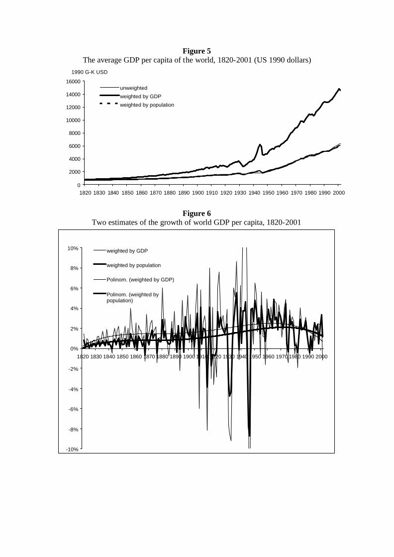
Figure 5 The average GDP per capita of the world, 1820-2001 (US 1990 dollars)

0

2000

4000

6000

8000

10000

12000

14000

16000

1820 1830 1840 1850 1860 1870 1880 1890 1900 1910 1920 1930 1940 1950 1960 1970 1980 1990 2000

unweighted

weighted by GDP

weighted by population

1990 G-K USD

Figure 6

Two estimates of the growth of world GDP per capita, 1820-2001

-10%

-8%

-6%

-4%

-2%

0%

2%

4%

6%

8%

10%

1820 1830 1840 1850 1860 1870 1880 1890 1900 1910 1920 1930 1940 1950 1960 1970 1980 1990 2000

weighted by GDP

weighted by population

Polinom. (weighted by GDP)

Polinom. (weighted bypopulation)

Table 2

Average annual growth rate of the GDP per capita Weighted by GDP Weighted by population Difference

1820-1870 1.11% 0.53% 0.58% 1871-1913 1.70% 1.22% 0.48% 1914-1950 1.81% 1.01% 0.80% 1950-1973 2.70% 2.67% 0.03% 1974-2001 1.44% 1.47% -0.03%

These patterns seem to confirm the assumptions of the Lucas model: there is a gradual acceleration of the growth of world GDP – broken by the exogenous shocks of the 1914-1950 period – followed by a deceleration of growth at the end of the 20th century. Moreover, the two patterns distinguished here – based on weighting by GDP and by population – seem to confirm the prediction of the model in terms of the development of global inequality as well. We will now review the trends in global inequality more in detail. 5. Global inequality These tentative results can easily be verified by calculating different measures of inequality on the basis of the amended Maddison dataset. We concentrate on the coefficient of variation, which is the standard deviation divided by the average and therefore measures relative inequality. A problem with these measures is that countries vary in size and therefore cannot be seen as single observations, and should have an impact on the standard deviation and the coefficient of variation related to their size. Moreover, as we already saw, this size can be either measured in terms of population and in terms of total GDP, and this choice may have implications for the results. So we get three different ways of measuring the development of inequality: the unweighted coefficient of variation (all countries have the same impact), and coefficients of variation weighted by population and weighted by GDP. This can moreover be done in two ways: when calculating the coefficient of variation we can divide the standard deviation by the average global GDP (per capita) – which is usually weighted by GDP – or we can divide the standard deviation by the related average – so the unweighted standard deviation is divided by the unweighted average GDP per capita, and the standard deviation which uses population weights is divided by the average GDP per capita weighted by population size. The second procedure, which is in our view the correct one, gives the results of Figure 7.

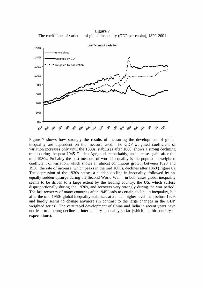
Figure 7

The coefficient of variation of global inequality (GDP per capita), 1820-2001

0%

20%

40%

60%

80%

100%

120%

140%

160%

1820

1830

1840

1850

1860

1870

1880

1890

1900

1910

1920

1930

1940

1950

1960

1970

1980

1990

2000

unweighted

weighted by GDP

weighted by population

coefficient of variation

Figure 7 shows how strongly the results of measuring the development of global inequality are dependent on the measure used. The GDP-weighted coefficient of variation increases only until the 1880s, stabilizes after 1880, shows a strong declining trend during the post-1945 Golden Age, and, remarkably, an increase again after the mid 1980s. Probably the best measure of world inequality is the population weighted coefficient of variation, which shows an almost continuous growth between 1820 and 1930; the rate of increase, which peaks in the mid 1800s, declines after 1860 (Figure 8). The depression of the 1930s causes a sudden decline in inequality, followed by an equally sudden upsurge during the Second World War – in both cases global inequality seems to be driven to a large extent by the leading country, the US, which suffers disproportionally during the 1930s, and recovers very strongly during the war period. The fast recovery of many countries after 1945 leads to certain decline in inequality, but after the mid 1950s global inequality stabilizes at a much higher level than before 1929, and hardly seems to change anymore (in contrast to the large changes in the GDP weighted series). The very rapid development of China and India in recent years have not lead to a strong decline in inter-country inequality so far (which is a bit contrary to expectations).

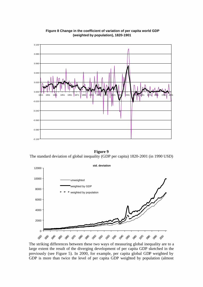
Figure 8 Change in the coefficient of variation of per capita world GDP (weighted by population), 1820-1901

-0.100

-0.080

-0.060

-0.040

-0.020

0.000

0.020

0.040

0.060

0.080

0.100

1821 1831 1841 1851 1861 1871 1881 1891 1901 1911 1921 1931 1941 1951 1961 1971 1981 1991 2001

Figure 9

The standard deviation of global inequality (GDP per capita) 1820-2001 (in 1990 USD)

0

2000

4000

6000

8000

10000

12000

1820

1830

1840

1850

1860

1870

1880

1890

1900

1910

1920

1930

1940

1950

1960

1970

1980

1990

2000

unweighted

weighted by GDP

weighted by population

std. deviation

The striking differences between these two ways of measuring global inequality are to a large extent the result of the diverging development of per capita GDP sketched in the previously (see Figure 5). In 2000, for example, per capita global GDP weighted by GDP is more than twice the level of per capita GDP weighted by population (almost

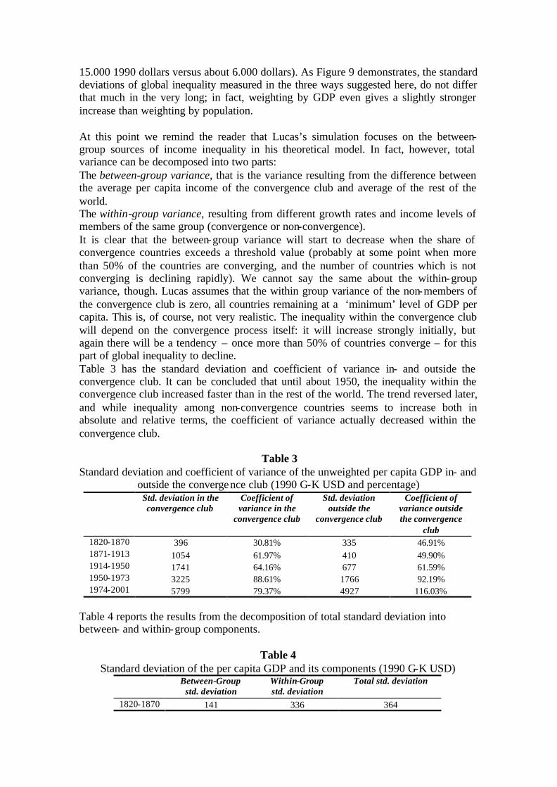
15.000 1990 dollars versus about 6.000 dollars). As Figure 9 demonstrates, the standard deviations of global inequality measured in the three ways suggested here, do not differ that much in the very long; in fact, weighting by GDP even gives a slightly stronger increase than weighting by population. At this point we remind the reader that Lucas’s simulation focuses on the between-group sources of income inequality in his theoretical model. In fact, however, total variance can be decomposed into two parts: The between-group variance, that is the variance resulting from the difference between the average per capita income of the convergence club and average of the rest of the world. The within-group variance, resulting from different growth rates and income levels of members of the same group (convergence or non-convergence). It is clear that the between-group variance will start to decrease when the share of convergence countries exceeds a threshold value (probably at some point when more than 50% of the countries are converging, and the number of countries which is not converging is declining rapidly). We cannot say the same about the within-group variance, though. Lucas assumes that the within group variance of the non-members of the convergence club is zero, all countries remaining at a ‘minimum’ level of GDP per capita. This is, of course, not very realistic. The inequality within the convergence club will depend on the convergence process itself: it will increase strongly initially, but again there will be a tendency – once more than 50% of countries converge – for this part of global inequality to decline. Table 3 has the standard deviation and coefficient of variance in- and outside the convergence club. It can be concluded that until about 1950, the inequality within the convergence club increased faster than in the rest of the world. The trend reversed later, and while inequality among non-convergence countries seems to increase both in absolute and relative terms, the coefficient of variance actually decreased within the convergence club.

Table 3 Standard deviation and coefficient of variance of the unweighted per capita GDP in- and

outside the convergence club (1990 G-K USD and percentage) Std. deviation in the

convergence club Coefficient of variance in the

convergence club

Std. deviation outside the

convergence club

Coefficient of variance outside the convergence

club 1820-1870 396 30.81% 335 46.91% 1871-1913 1054 61.97% 410 49.90% 1914-1950 1741 64.16% 677 61.59% 1950-1973 3225 88.61% 1766 92.19% 1974-2001 5799 79.37% 4927 116.03%

Table 4 reports the results from the decomposition of total standard deviation into between- and within-group components.

Table 4 Standard deviation of the per capita GDP and its components (1990 G-K USD)

Between-Group std. deviation

Within-Group std. deviation

Total std. deviation

1820-1870 141 336 364

1871-1913 420 701 817 1914-1950 751 1117 1346 1950-1973 857 2656 2791 1974-2001 1385 5153 5336

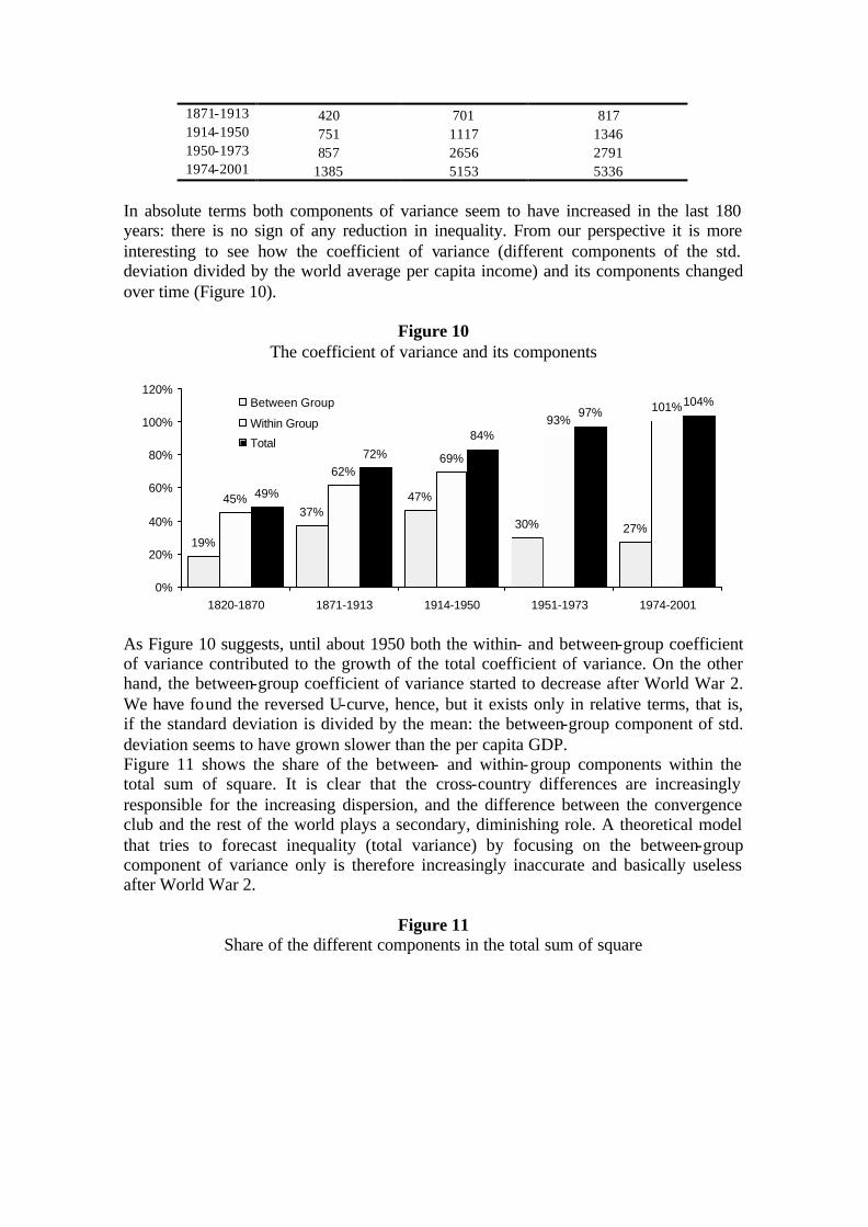
In absolute terms both components of variance seem to have increased in the last 180 years: there is no sign of any reduction in inequality. From our perspective it is more interesting to see how the coefficient of variance (different components of the std. deviation divided by the world average per capita income) and its components changed over time (Figure 10).

Figure 10 The coefficient of variance and its components

19%

37%47%

30% 27%

45%

62%69%

93%101%

49%

72%

84%

97%104%

0%

20%

40%

60%

80%

100%

120%

1820-1870 1871-1913 1914-1950 1951-1973 1974-2001

Between Group

Within Group

Total

As Figure 10 suggests, until about 1950 both the within- and between-group coefficient of variance contributed to the growth of the total coefficient of variance. On the other hand, the between-group coefficient of variance started to decrease after World War 2. We have found the reversed U-curve, hence, but it exists only in relative terms, that is, if the standard deviation is divided by the mean: the between-group component of std. deviation seems to have grown slower than the per capita GDP. Figure 11 shows the share of the between- and within-group components within the total sum of square. It is clear that the cross-country differences are increasingly responsible for the increasing dispersion, and the difference between the convergence club and the rest of the world plays a secondary, diminishing role. A theoretical model that tries to forecast inequality (total variance) by focusing on the between-group component of variance only is therefore increasingly inaccurate and basically useless after World War 2.

Figure 11 Share of the different components in the total sum of square

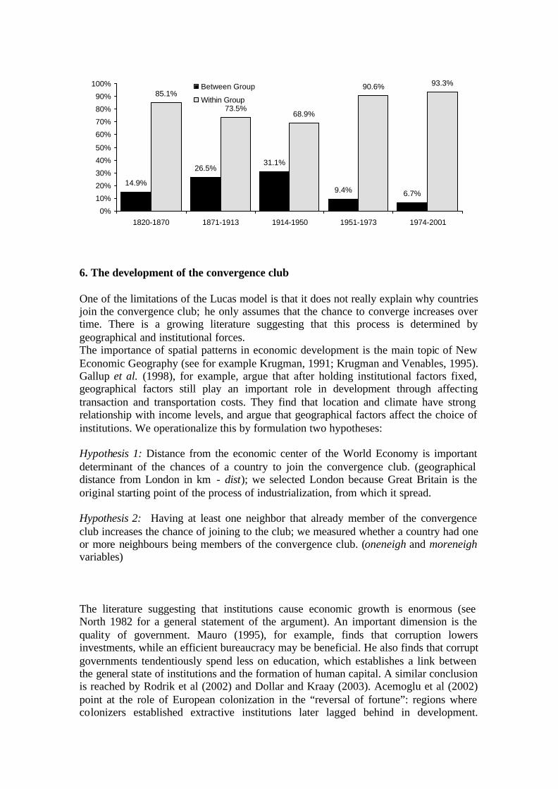
14.9%

26.5%31.1%

9.4% 6.7%

85.1%

73.5%68.9%

90.6% 93.3%

0%

10%

20%

30%

40%

50%

60%

70%

80%

90%

100%

1820-1870 1871-1913 1914-1950 1951-1973 1974-2001

Between Group

Within Group

6. The development of the convergence club One of the limitations of the Lucas model is that it does not really explain why countries join the convergence club; he only assumes that the chance to converge increases over time. There is a growing literature suggesting that this process is determined by geographical and institutional forces. The importance of spatial patterns in economic development is the main topic of New Economic Geography (see for example Krugman, 1991; Krugman and Venables, 1995). Gallup et al. (1998), for example, argue that after holding institutional factors fixed, geographical factors still play an important role in development through affecting transaction and transportation costs. They find that location and climate have strong relationship with income levels, and argue that geographical factors affect the choice of institutions. We operationalize this by formulation two hypotheses: Hypothesis 1: Distance from the economic center of the World Economy is important determinant of the chances of a country to join the convergence club. (geographical distance from London in km - dist); we selected London because Great Britain is the original starting point of the process of industrialization, from which it spread. Hypothesis 2: Having at least one neighbor that already member of the convergence club increases the chance of joining to the club; we measured whether a country had one or more neighbours being members of the convergence club. (oneneigh and moreneigh variables) The literature suggesting that institutions cause economic growth is enormous (see North 1982 for a general statement of the argument). An important dimension is the quality of government. Mauro (1995), for example, finds that corruption lowers investments, while an efficient bureaucracy may be beneficial. He also finds that corrupt governments tendentiously spend less on education, which establishes a link between the general state of institutions and the formation of human capital. A similar conclusion is reached by Rodrik et al (2002) and Dollar and Kraay (2003). Acemoglu et al (2002) point at the role of European colonization in the “reversal of fortune”: regions where colonizers established extractive institutions later lagged behind in development.

Another set of institutions – ‘communism’ or a centrally planned economy – has also been subject to much debate; did communism hinder economic development in (for example) Russia and Eastern Europe, or make it possible to industrialize rapidly and enter the convergence club, as Allen (2003) has argued for the Soviet Union?

The direction of causality between welfare and institutions is not obvious, however. Lipset (1960) argues that rising welfare paired with the improvement of human capital leads to better institutions and conflict solving mechanisms. His view is opposed by Przeworski and Limongi (1993, 1994, 2004), who state that changes in political institutions are basically not determined by economic development, that is democracy may rise in any country independently whether it is wealthy or not. There is no endogeneity thus, but higher income may help to preserve democracy. These two hypotheses are of high importance for any empirical research in this area, since if Lipset is right, the coefficients from the regressions analyzing the relationship between institutions and economic growth are likely to be biased. Glaeser et al. (2004) find that the causality link cannot be easily determined, and the positive relationship between democracy and economic performance is not necessarily general: autocratic regimes may foster economic growth up to the point enough human capital is accumulated for a change in political system to take place. Milanovic (2005), similarly to this paper, relies on the Maddison and the PolityIV datasets to test the hypothesis whether higher income increases the chance of changing to democracy. He points out that the relationship between democracy and income depends largely on out definition what democracy is. If we are very narrow in our hypothesis, there is a positive relationship between income and democracy and Lipset’s hypothesis can be justified. If the previously achieved level of democracy is taken account with, though, the level of income loses its importance. This leads us to formulate the following hypotheses: Hypothesis 3: Political institutions are important determinants whether a country converges to the leader. We measure the quality of policy using the PolityIV variable from (http://www.cidcm.umd.edu/inscr/polity/) (a high number means more democratic regime). Hypothesis 4: Communism – i.e. a centrally planned economy – was an instrument for entering the convergence club (a communism dummy should have a positive sign) Hypothesis 5: Colonization has a negative impact on a country’s chance to converge. (colony variable)3 A variable that is at the crossroads between institutions and geography is the settler dummy.4 Acemoglu et.al.(2002) argues that Europeans introduced different institutions depending on the hospitability of environment and the wealth of the subdued region. In hospitable but poor regions they founded settler colonies with more European- like 3 Since the Polity IV dataset follows the historical changes in borders and countries, we had to adjust it to the Maddison dataset that projects today’s countries back in time. This was especially required for developing countries that did not exist or were colonies before World War 2. For the extrapolation of the missing data, we used the following strategy: colonies were given the same polity score as their metropoles. (The additional, probably negative, effect of colonization is captured by the colony dummy in the regressions.) For countries that were independent, we used the scores of similar countires. For example in South-East Asia, we used the Chinese score (-6), while in case of the African tribal kingdoms, we took the average of China (-6) and Turkey(-10): -8. 4 USA, Canada, Australia, New Zealand, Argentina, Brazil, Chile, Uruguay, South Africa, Hong Kong.

institutions, while in rich or hostile areas they rather applied extractive institutions. Acemoglu et al. suggest these institutional differences were decisive in the later development of the ex-colonies, leading to the large-scale differences in welfare observed today. The expected sign of the settler coefficient is positive. Specification

{ }

i,t 0 1 i,t 2 i 3 i,t 4 i,t

5 i,t 6 i 7 i,t i t i,t

i,t i,t i , t i,t

Y polity lndist oneneigh moreneigh

communism settler colony

Y member , join ,leave

= α + α + α + α + α +

+α + α + α + η + τ + ε

=

(1.)

where ?i, and t t denote the country, and period specific unobserved effects, and ei,t is the error-term assumed to be i.i.d.. We assume the strict exogeneity of the regressors. The variables are summarized in the following table:

Variable Description Variable Description memberi,t, joini,t, leavei,t

Binary dependent variables 1 if country i was member

of/joined/left the convergence club in period t, 0 otherwise

moreneighi,t 1 if country i had more than one neighbor in the

convergence club in period t, 0 otherwise

polityi,t Polity score of country i in period t ranging between -10

and +10.

communismi,t 1 if country i was colony, 0 otherwise

lndisti Logarithm of the distance of country i from London in km.

settleri 1 if country i was a settler colony

oneneighi,t 1 if country i had at least one neighbor in the convergence club in period t, 0 otherwise

colonyi,t 1 if country i was a colony in period t, 0

otherwise We estimated equation (1.) in both random-effect and fixed-effect specification. In the fixed-effect specification we applied the method suggested by Mundlak (1978).5 This allows us to estimate the coefficients of the time- invariant regressors as well. The results for the different periods are summarized in the next table. The marginal impacts are calculated at the mean of the dependent variable.6 Originally, we planned to apply different colony dummies for different metropoles to capture the difference in colonial policies, but since these turned out to be insignifcant (with t-statistics near zero), or were sometimes dropped, we opted for using a single colony dummy. The chance of being in the convergence club

5 Instead of subtracting the country specific mean of variables from both sides (Within-Group transformation), he suggests using these means as regressors. These coefficients are not reported in the tables as they have no economic importance. The advantage of the method is that it requires no transformation of the data, and it is possible to estimate the coefficients of time -invariant regressors. Their presence, however, marginally increases the pseudo-R2. 6 We used the logit function of the Stata, together with the mfx function that calculates the marginal impacts with significance tests. We opted not to use xtlogit, because it does not calculate robust t-statistics, and has the tendency to drop dummy variables on ground that they predict perfect success or failure, even though theoretically these variables are also important.

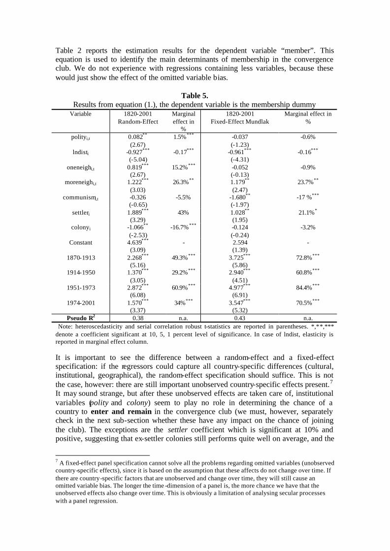
Table 2 reports the estimation results for the dependent variable “member”. This equation is used to identify the main determinants of membership in the convergence club. We do not experience with regressions containing less variables, because these would just show the effect of the omitted variable bias.

Table 5. Results from equation (1.), the dependent variable is the membership dummy

Variable 1820-2001 Random-Effect

Marginal effect in

%

1820-2001 Fixed-Effect Mundlak

Marginal effect in %

polityi,t 0.082** (2.67)

1.5%*** -0.037 (-1.23)

-0.6%

lndisti -0.927*** (-5.04)

-0.17*** -0.961***

(-4.31) -0.16***

oneneighi,t 0.819*** (2.67)

15.2%*** -0.052 (-0.13)

-0.9%

moreneighi,t 1.222*** (3.03)

26.3%** 1.179** (2.47)

23.7%**

communismi,t -0.326 (-0.65)

-5.5% -1.680** (-1.97)

-17 %***

settleri 1.889*** (3.29)

43% 1.028** (1.95)

21.1%*

colonyi -1.066** (-2.53)

-16.7%*** -0.124 (-0.24)

-3.2%

Constant 4.639*** (3.09)

- 2.594 (1.39)

-

1870-1913 2.268*** (5.16)

49.3%*** 3.725*** (5.86)

72.8%***

1914-1950 1.370*** (3.05)

29.2%*** 2.940*** (4.51)

60.8%***

1951-1973 2.872*** (6.08)

60.9%*** 4.977*** (6.91)

84.4%***

1974-2001 1.570*** (3.37)

34%*** 3.547*** (5.32)

70.5%***

Pseudo R2 0.38 n.a. 0.43 n.a. Note: heteroscedasticity and serial correlation robust t-statistics are reported in parentheses. *,**,*** denote a coefficient significant at 10, 5, 1 percent level of significance. In case of lndist, elasticity is reported in marginal effect column. It is important to see the difference between a random-effect and a fixed-effect specification: if the regressors could capture all country-specific differences (cultural, institutional, geographical), the random-effect specification should suffice. This is not the case, however: there are still important unobserved country-specific effects present.7 It may sound strange, but after these unobserved effects are taken care of, institutional variables (polity and colony) seem to play no role in determining the chance of a country to enter and remain in the convergence club (we must, however, separately check in the next sub-section whether these have any impact on the chance of joining the club). The exceptions are the settler coefficient which is significant at 10% and positive, suggesting that ex-settler colonies still performs quite well on average, and the

7 A fixed-effect panel specification cannot solve all the problems regarding omitted variables (unobserved country-specific effects), since it is based on the assumption that these affects do not change over time. If there are country-specific factors that are unobserved and change over time, they will still cause an omitted variable bias. The longer the time -dimension of a panel is, the more chance we have that the unobserved effects also change over time. This is obviously a limitation of analysing secular processes with a panel regression.

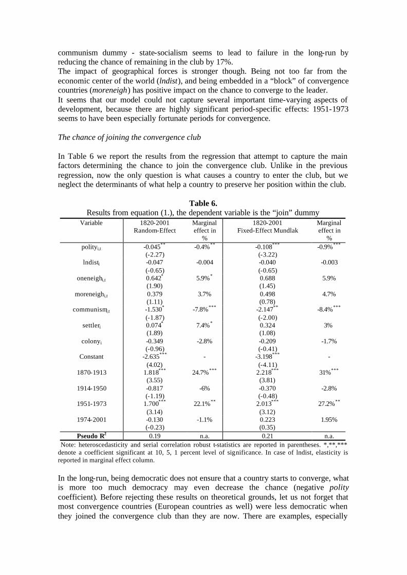
communism dummy - state-socialism seems to lead to failure in the long-run by reducing the chance of remaining in the club by 17%. The impact of geographical forces is stronger though. Being not too far from the economic center of the world (lndist), and being embedded in a “block” of convergence countries (moreneigh) has positive impact on the chance to converge to the leader. It seems that our model could not capture several important time-varying aspects of development, because there are highly significant period-specific effects: 1951-1973 seems to have been especially fortunate periods for convergence. The chance of joining the convergence club In Table 6 we report the results from the regression that attempt to capture the main factors determining the chance to join the convergence club. Unlike in the previous regression, now the only question is what causes a country to enter the club, but we neglect the determinants of what help a country to preserve her position within the club.

Table 6. Results from equation (1.), the dependent variable is the “join” dummy

Variable 1820-2001 Random-Effect

Marginal effect in

%

1820-2001 Fixed-Effect Mundlak

Marginal effect in

% polityi,t -0.045**

(-2.27) -0.4%** -0.108***

(-3.22) -0.9%***

lndisti -0.047 (-0.65)

-0.004 -0.040

(-0.65) -0.003

oneneighi,t 0.642* (1.90)

5.9%* 0.688 (1.45)

5.9%

moreneighi,t 0.379 (1.11)

3.7% 0.498 (0.78)

4.7%

communismi,t -1.530* (-1.87)

-7.8%*** -2.147** (-2.00)

-8.4%***

settleri 0.074* (1.89)

7.4%* 0.324 (1.08)

3%

colonyi -0.349 (-0.96)

-2.8% -0.209 (-0.41)

-1.7%

Constant -2.635*** (4.02)

- -3.198*** (-4.11)

-

1870-1913 1.818*** (3.55)

24.7%*** 2.218*** (3.81)

31%***

1914-1950 -0.817 (-1.19)

-6% -0.370 (-0.48)

-2.8%

1951-1973 1.700*** (3.14)

22.1%** 2.013*** (3.12)

27.2%**

1974-2001 -0.130 (-0.23)

-1.1% 0.223 (0.35)

1.95%

Pseudo R2 0.19 n.a. 0.21 n.a. Note: heteroscedasticity and serial correlation robust t-statistics are reported in parentheses. *,**,*** denote a coefficient significant at 10, 5, 1 percent level of significance. In case of lndist, elasticity is reported in marginal effect column. In the long-run, being democratic does not ensure that a country starts to converge, what is more too much democracy may even decrease the chance (negative polity coefficient). Before rejecting these results on theoretical grounds, let us not forget that most convergence countries (European countries as well) were less democratic when they joined the convergence club than they are now. There are examples, especially

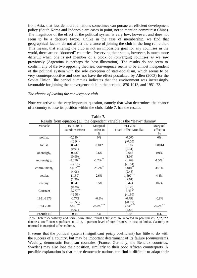
from Asia, that less democratic nations sometimes can pursue an efficient development policy (South Korea and Indonesia are cases in point, not to mention communist China). The magnitude of the effect of the political system is very low, however, and does not seem to be a decisive factor. Unlike in the case of membership, we find that geographical factors do not affect the chance of joining the club in the long-run either. This means, that entering the club is not an impossible goal for any countries in the world, there are no “doomed” countries. Preserving their status, however, is much more difficult when one is not member of a block of converging countries as we saw previously (Argentina is perhaps the best illustration). The results do not seem to confirm any of the two opposing theories: convergence seems to be almost independent of the political system with the sole exception of state-socialism, which seems to be very counterproductive and does not have the effect postulated by Allen (2003) for the Soviet Union. The period dummies indicates that the environment was increasingly favourable for joining the convergence club in the periods 1870-1913, and 1951-73. The chance of leaving the convergence club Now we arrive to the very important question, namely that what determines the chance of a country to lose its position within the club. Table 7. has the results.

Table 7. Results from equation (1.), the dependent variable is the “leave” dummy

Variable 1914-2001 Random-Effect

Marginal effect in

%

1914-2001 Fixed-Effect Mundlak

Marginal effect in

% polityi,t -0.030**

(-0.94) 0% -0.000

(-0.00) 0%

lndisti 0.247 (0.91)

0.012 0.107

(0.31) 0.0014

oneneighi,t 0.437 (0.99)

0.6% 0.646 (1.03)

0.9%

moreneighi,t -2.096** (-2.18)

-1.7%** -1.769 (-1.54)

-1.5%*

communismi,t 3.487*** (4.06)

28.2%* 3.810** (2.48)

38.1%

settleri 1.130* (1.90)

2.6% 1.597*** (2.61)

4.4%

colonyi 0.341 (0.38)

0.5% 0.424 (0.33)

0.6%

Constant .5.777** (-2.59)

- -5.437* (-1.80)

-

1951-1973 -0.773 (-0.58)

-0.9% -0.793 (-0.55)

-0.8%

1974-2001 3.871*** (5.97)

23.6%*** 3.845*** (4.85)

22.2%**

Pseudo R2 0.44 n.a. 0.45 n.a. Note: heteroscedasticity and serial correlation robust t-statistics are reported in parentheses. *,**,*** denote a coefficient significant at 10, 5, 1 percent level of significance. In case of lndist, elasticity is reported in marginal effect column. It seems that the political system (insignificant polity coefficient) has little to do with the success of a country, but may be important determinant of its failure (communism). Wealthy, democratic European countries (France, Germany, the Benelux countries, Sweden) may also lose their position, similarly to their poor African counterparts. A possible explanation is that more democratic nations can find it difficult to adapt their

social security systems and welfare institutions to changing environment. Here the stabilization process may take a long time, and during this time even a wealthy country may lag behind the leader (USA). Being close to a block of convergence club (significant negative moreneigh coefficient) seems to offer a marginal protection from losing position, but this is not guarantee, as we saw in case of Western Europe after 1974. 7. Conclusion In this paper we have developed and tested the idea that the development of global inequality can be analysed as driven by the diffusion of the process of industrialization in the past two centuries. We used Lucas (2000) model as an elegant (but perhaps rather simple) way to operationalize this idea. The competing approach to global inequality, which we kept in the back of our mind but was not developed in more detail, is that the world economy is characterized by relative stable relationships core and periphery. We used a (slightly extended) version of the Maddison (2001) dataset to test the ideas of the Lucas model. The predictions of the model were threefold: (1) the share of countries or the share of the world population that is converging is constantly increasing, and these shares show a logistic curve approaching 100% in the long run; (2) global inequality (between countries) increases until more than 50% of countries/world population is member of the convergence club; afterwards, inter-country global inequality will begin to decline; and (3) the growth rate of world GDP will also increase during the first phase of the diffusion process until the majority of countries is converging, after which the growth of world GDP will start to decline again (until in the very long run they are all growing at the rate of the leading country). Our main results are as follows. The ‘bad news’ is that the share of countries converging is not growing consistently in time, in particular because after 1973 many countries seem to leave the convergence club, because they grow at a slower rate than the US and/or have a income per capita that is lower than 80% of the leading country. The failure of many countries to continue being member of the convergence club (as defined here) is probably the most striking ‘problem’; or put differently, the Lucas model does not allow countries to leave the convergence club, but in practice they do, and in particular many did after 1973. We have to be a bit cautious of course, because we do not know their long term performance after 1973; only in the 2020s or 30s, after another period of 30 years, can we really assess if this was a structural phenomenon or just a temporary set back, caused, for example, by the desintegration of the communist world and the transition problems faced by the centrally planned economies (many of which left of convergence club after 1973). Similarly, it is still rather early to judge the economic performance of the Western European countries (such as the Netherlands), or countries such as Australia that also left the club after 1973; between 1973 and the mid 1990s Western Europe increased its labour productivity faster than the US. At the same time its labour force and labour input grew much more slowly than in the US, causing a slower growth of per capita GDP. Whether this was a voluntary choice – the result of different preferences for leisure versus income – or the result of bad institutions and incentives in Western Europe is still a matter of debate.

The ‘good news’ is that the share of the world population converging is growing over time, and has continued to increase after 1973 (when a few very big countries such as India and China joined the club). In that – more important – respect our data seem to be consistent with the predictions of the Lucas model, albeit that the share of the world population converging does not show the logistic growth curve that results from the

model. During the 19th century this appeared to be the case, but the world wars and great depression of the 1930s ‘breaks’ the pattern found, and led to a near-stabilization of the share of the world population converging, whereas one would have expected - on the basis of the 19th century pattern – a further, even accelerated growth of that share. The convergence club (in terms of world population) again expanded consistent ly after 1945 (although this is to some extent also dependent on the classification of China, which does not enter the convergence club until 1973), as a result of which in the most recent period (1974-2001) more than 60% of world population is converging (and this excludes a large part of Western Europe and Australia, which discontinued converging after 1973). Global inequality (between countries) seems to move more or less in line with the expectations of the Lucas model. It increased strongly in the century and a half after the start of the Industrial Revolution, and only began to stabilize in the second half of the 20th century (see Boltho and Toniolo (1999) for a similar result). We could also establish that the increase in global inequality was most rapid during the middle decades of the 19th century – when only a few countries industrialized rapidly – and already began to slow down during the first phase of globalization after 1870 (which was indeed a very successful period of the spread of ‘modern economic growth’) (although it should be added that the data for the pre 1913 period are much weaker than for the 20th century). But, in spite of the fact that more than 60% of the world population is now part of the ‘convergence club’, we see no signs of a continuing decline of global inequality yet. In fact, the new growth spurt set in by the US after the mid 1990s, and the continuing bad performance of Africa (and Latin America, and GOS countries), seems to counterbalance the strong performance of East and South-Asian countries such as India and China. Also the prediction that the growth of world GDP is most rapid when about 50% of world population is converging, appears at first sight to be consistent with the facts as reconstructed here, in view of the acceleration of growth after 1945. But the post 1973 slowing down of world growth cannot be easily explained in there terms – such a slowing down might only happen when a large majority of the world population is close to convergence, which obviously is not the case (yet). The most obvious problem with the Lucas model is that it does not explain why countries enter (or leave) the club. We have tried to find out which spatial and institutional factors determine this process. It can be concluded that geography plays a very important role in this – that closeness to London and having neighbors who are also part of the convergence club are important factors in determining once position – being a member or not. It proved more difficult to establish the role played by institutions – only communism was consistently a negative factor in terms of the chance of being or becoming a member of the convergence club, and also increased the chance to leave the club.

References

Acemoglu, D., Johnson S. and Robinson J. (2002): Reversal of Fortune: Geography and Institutions in the Making of the Modern World Income Distribution, Quarterly Journal of Economics 117(4), 1231-1294. Aghion, P and Howitt, P (1992): A Model of Growth through Creative Destruction. Econometrica 60, 323-351 Allen, R.C. (2003) From Farm to Factory: a reinterpretation of the Soviet Industrial Revolution. Princeton: Princeton U.P. Boltho, A. and Toniolo, G. (1999): The assessment: the Twentieth century – Achievements, Failures, Lessons, Oxford Review of Economic Policy, 15 (4) 1-17. Crafts, N.F.R. (2004) The world economy in the 1990s: a long run perspective. LSE Working papers in Economic History, no. 87/04. Dollar, D. and Kraay, A. (2003): Institutions, Trade and Growth, Journal of Monetary Economics 50(1), 133-62. Dowrick, S. and DeLong, J. B. (2003): Globalization and Convergence, in Jeffrey Williamson (ed.), Globalization in Historical Perspective, Chicago: University of Chicago Press Gallup, J. L., Sachs, J.D., and Mellinger, A. D. (1998): Geography and Economic Development , NBER Working Paper No. 6849 Glaeser, E. L., La Porta, R., Lopez-de-Silanes, F. and Shleifer, A. (2004): Do Institutions Cause Growth? , NBER Working Paper No. 10568 Holz, C.A. (2006): China’s reform period economic growth. Review of Income and Wealth, 52 (1), …. King, R. G. and Levine R. (1993): Finance and Growth: Schumpeter Might be Right, Quarterly Journal of Economics 108(3), 717-737. Lipset, S. M. (1960): Political Man: The Social Basis of Modern Politics. New York: Doubleday Lucas, R. E. (1988): On the Mechanics of Economic Development. Journal of Monetary Economics 22(1), 3-42. Lucas, R. E. (2000), Some Macroeconomics for the 21st Century, Journal of Economic Perspectives 14, 159-168. Krugman, P. (1991), Increasing Returns and Economic Geography, Journal of Political Economy, 99, 483–99.

Krugman, P. and Venables, A. J. (1995), Globalization and the Inequality of Nations, Quarterly Journal of Economics, 110(4), 857–80. Maddison, A. (2001): The World Economy: A millennial perspective. Paris: OECD. Milanovic, B. (2005): Relationship between Income and Emergence of Democracy Reexamined, 1820-2000: A non-parametric approach. Mimeo. Przeworski, A. and Limongi, F. (1993): Political regimes and Economic Growth, Journal of Economic Perspectives 7, 25-46. Przeworski, A. and Limongi, F. (1997): Modernization: Theories and facts, World Politics 49(2), 155-183. Przeworski, A. (2004): Capitalism, development and democracy, Revista de Economia Politica 24(4) Rodrik, D., Subramanian, A. and Trebbi, F. (2002): Institutions Rule: The Primacy of Institutions over Geography and Integration in Economic Development. NBER Working Paper No. 9305 Romer, P. M. (1986): Increasing Returns and Long Run Growth, Journal of Political Economy 94(5), 1002-1037. Romer, P. M. (1990): Endogenous Technological Change, Journal of Political Economy 98(5), 71-102. Solow, R. M. (1956): A Contribution to the Theory of Economic Growth, Quarterly Journal of Economics 70(1), 65-94. Tamura (1996) Wallerstein, I. (1974): The Modern World System, I. New York: Academic Press.

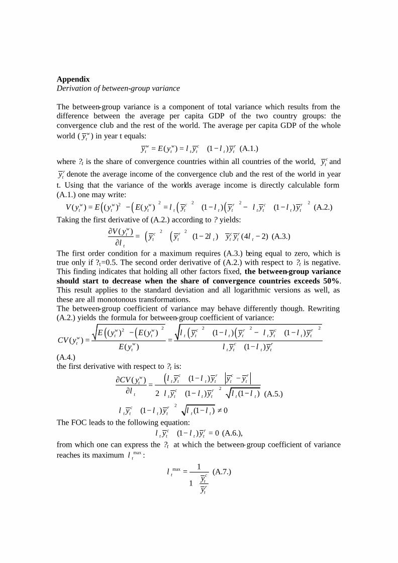
Appendix Derivation of between-group variance The between-group variance is a component of total variance which results from the difference between the average per capita GDP of the two country groups: the convergence club and the rest of the world. The average per capita GDP of the whole world ( w

ty ) in year t equals:

( ) (1 )w w c rt t t t t ty E y y yλ λ= = + − (A.1.)

where ?t is the share of convergence countries within all countries of the world, cty and

rty denote the average income of the convergence club and the rest of the world in year

t. Using that the variance of the worlds average income is directly calculable form (A.1.) one may write:

( ) ( ) ( ) ( )2 2 2 22( ) ( ) ( ) (1 ) (1 )w w w c r c rt t t t t t t t t t tV y E y E y y y y yλ λ λ λ = − = + − − + − (A.2.)

Taking the first derivative of (A.2.) according to ? yields:

( ) ( )2 2( )(1 2 ) (4 2)

wc r c rtt t t t t t

t

V yy y y yλ λ

λ∂ = + − + − ∂

(A.3.)

The first order condition for a maximum requires (A.3.) being equal to zero, which is true only if ?t=0.5. The second order derivative of (A.2.) with respect to ?t is negative. This finding indicates that holding all other factors fixed, the between-group variance should start to decrease when the share of convergence countries exceeds 50%. This result applies to the standard deviation and all logarithmic versions as well, as these are all monotonous transformations. The between-group coefficient of variance may behave differently though. Rewriting (A.2.) yields the formula for between-group coefficient of variance:

( ) ( ) ( ) ( )2 2 2 22( ) ( ) (1 ) (1 )( )

( ) (1 )

w w c r c rt t t t t t t t t tw

t w c rt t t t t

E y E y y y y yCV y

E y y y

λ λ λ λ

λ λ

− + − − + − = =+ −

(A.4.) the first derivative with respect to ?t is:

( )2

2

(1 )( )

2 (1 ) (1 )

(1 ) (1 ) 0

+ − ⋅ −∂=

∂ + − ⋅ −

+ − ⋅ − ≠

c r c rwt t t t t tt

c rt t t t t t t

c rt t t t t t

y y y yCV y

y y

y y

λ λ

λ λ λ λ λ

λ λ λ λ

(A.5.)

The FOC leads to the following equation: (1 ) 0c r

t t t ty yλ λ+ − = (A.6.), from which one can express the ?t at which the between-group coefficient of variance reaches its maximum max

tλ :

max 1

1t c

trt

yy

λ =+

(A.7.)

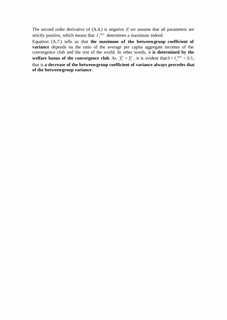
The second order derivative of (A.4.) is negative if we assume that all parameters are strictly positive, which means that max

tλ determines a maximum indeed. Equation (A.7.) tells us that the maximum of the between-group coefficient of variance depends on the ratio of the average per capita aggregate incomes of the convergence club and the rest of the world. In other words, it is determined by the welfare bonus of the convergence club. As c r

t ty y> , it is evident that max0 0.5tλ< < , that is a decrease of the between-group coefficient of variance always precedes that of the between-group variance.