global insight's apt stock sector forecasting model insight's apt stock sector forecasting...
TRANSCRIPT

Copyright © 2005 Global Insight
1
Global Insight's APT Stock Sector Forecasting Model Mark Killion, CFA
Natasha Muravytska February 2005
Introduction Global Insight's World Industry Service (WIS) has recently developed an "APT-style" model for use in sector-based asset management. This is a practical forecasting model created to provide a fundamental basis for quantitative portfolio construction and asset allocation, by helping to select the "optimal" over- and under-weight positions for sectors in a portfolio relative to those in the benchmark. Historical simulations show this framework can provide significant "out performance" of the sector optimized portfolio relative to the total market performance. This model forecasts the year-ahead expected total return to be gained (or lost) by owning shares in publicly traded companies, when those companies are added together into "peer groups" of stock market sectors. The data forecasted are the total sector returns for each of the 10 broad GICS-based economic sectors that comprise the total market. Then, the model adds each of the sectors into a result for the S&P500 total benchmark. The model-generated expected returns for sectors are then used in conjunction with portfolio optimization procedures to derive recommended over- or under-weight position of sectors in the portfolio, as compared to the sector weights that are in the benchmark used to measure the portfolio. Although the APT model does generate point forecasts of expected future returns for stock sectors, this framework relies upon the relative distribution of the expected returns among stock market sectors to drive the optimal sector weights for a portfolio. Used in this manner, the framework can reliably advise asset managers on the best sector composition of their stock market investment portfolios that will maximize their total return. This model only addresses the US stock market. Research from others indicate that it can be extended, and indeed improved, by the inclusion of European, Asian, and other major stock markets around the world; but this exercise is left for a future endeavor. Model Summary This model is based upon the Arbitrage Pricing Theory (APT) that shows how current known data from "today" has strong predictive power for "future" stock market returns—a lead-lag relationship (see Appendix 1 for Theoretical Background). We have replicated and then extended the classic APT model framework to better facilitate its use in practical applications, such as portfolio construction. Key attributes of our model include:
• Lead/Lag Relationships: Five-of-seven variables used to forecast returns are historical data
• Connect macro views and scenarios down to sector impacts and stock market behavior: This APT model simulates macro performances down through sector impacts to derive the expected changes in the asset value of stock investment portfolios

Copyright © 2005 Global Insight
2
• Highlights Global Insight information: all data come from: World Industry Service (WIS); US Macro Economic Service; or the SANDP (S&P) historical data bank
• Portfolio simulation/advisory: The model provides a framework for using fundamental factors to simulate and forecast portfolios to serve as basis for advisory, such as "over weighting" or "under weighting" sectors relative to the overall benchmark
Model Specification The metrics used in most APT models to generate expected returns are fundamental indicators of valuation and profitability, such as the Dividend Yield, Dividend Payout Ratios, and the Price to Earnings (P/E) Ratio. In line with this, in Global Insight's WIS APT Stock Sector Forecasting model, higher expected total returns are generated by higher dividend payout ratios and higher dividend yields. In addition, we have enhanced the traditional APT specification to include indicators such as free cash flow and the interest rate "yield curve." So, in our model higher free cash flow and a steeper (higher) yield curve also generate higher expected returns. By contrast, the "PEG" ratio indicator carries a negative sign in this model, so that a higher current PEG ratio forecasts lower future total returns. (The PEG ratio is created by dividing current sector P/E ratios by three-year forward growth rates in same sector profits—see Appendix 2 for more details). Higher current stock prices relative to trailing earnings push up P/E ratios and, thus, the PEG (lowering expected return); while higher expected growth in future profits lowers the PEG (raising expected return). This sort of model specification is closely aligned with the "Value" and "GAARP" approaches to stock market investing:
• buy at a low price and sell at a high price • look for fast earnings growth in the context of a reasonable price • recognize future portfolio returns will largely be determined by the dividends you receive • diversify the portfolio among different types of exposure • pay attention to management efficiency in the use of capital and investments • respect the monetary conditions as shown by policy interest rates and the yield curve • minimize your transaction and investment costs
Our Stock Sector APT model is specified in the same manner for each of the 10 Economic GICS®1 sectors: Energy, Basic Materials, Industrials, Consumer Discretionary, Consumer Staples, Healthcare, Financials, Information Technology, Telecommunications, and Utilities. We estimated the parameters in the 10 sector equations using well-known OLS regression techniques. The model is specified in a standard log format, and fit to the quarterly frequency time period from first-quarter 1995 through fourth-quarter 2004. The GICS framework for organizing sectors allows us to incorporate the latest, up-to-date sector peer group conventions and data observations in the model. However, one weakness of GICS-organized sector data is that the length of historical data is limited (GICS was only put in place in the late 1990s). Therefore, the availability of historical, quarterly frequency data for GICS-organized sectors in the S&P500 are not readily available prior to 1995.

Copyright © 2005 Global Insight
3
The (left-hand side) variable being explained by the model is the concept of "excess return," which is defined as the total return earned by the stock sector that is over and above the return that could be earned by simply investing in the relatively riskless three-month T-Bills. So, the WIS APT Stock Sector Forecasting model is specified as:
q[-4]YLD_SLOPE. *k .q[-4]FCF*k .q[-4]PEG_3y*k-
.q[-4]D_P *k _GR.q[-4]D_E*k kSector for Return Excess
5j4j3
j2j10
++
++=
Where: --Excess Return for Sector = ))(comp_3mtb*.q[-4]) /(.q jj TRITRI . --TRI—log of Sector Total Return measured as percent change from same quarter a year ago. --COMP_3MTB—log of the three-month T-Bill rate of return as compounded over four quarters. --D_E_GR—log of the Payout Ratio "turning point" indicator, which is the annual dividend payout ratio divided by a moving average of the previous three years' dividend payout ratio. --D_P—log of dividend yield level. --FCF—log of the Free Cash Flow "turning point" indicator, which is the annual free cash flow divided by a moving average of the previous three years' free cash flow; where:
Sector Free Cash Flow = Sector Profit – Sector Capital Expenditures. --PEG_3y—log of PEG Ratio, defined as the current P/E ratio (end of quarter value) divided by three-year forward earnings growth rates: PEG_3y = PE/3-year forward growth of earnings. --YLD_SLOPE—log of the Yield Slope, measured as a ratio between 10-year bond yields and three-month T-Bill rates. A ratio was used to accommodate the use of logs in model estimation. --[-4] Denotes a four quarter lag in the in the indicated variable in relation to the time period for the explained LHS variable. A detailed description of the data is featured in Appendix 2. The model coefficients and statistical measures of historical fit are presented in Appendix 3, which is available upon request to clients of Global Insight. Additional Features of Global Insight's APT Stock Sector Model This model replicates and then builds upon typical APT relationships used in previous research. This section highlights several areas of additional feature we have constructed in our version of the APT model. These enhancements were designed to better align the results with common conventions used in asset management, and so that the model-generated expected return can be used directly in the fundamental construction of portfolios. First, we have updated the model through recent years, to cover the 1994–2004 periods of boom, bust, and recovery. Previous research had largely used data from prior to 1998. Second, we have extended the model's predictive time frame from the typical one-quarter a-head view to a more practically useful four-quarter a-head view. Third, we followed the example of Fama and French to establish APT relationships at the level of sectors underneath market totals. Thus, our model forecasts year-ahead expected returns for stock market sectors.

Copyright © 2005 Global Insight
4
Fourth, we eliminated a typical weakness of previous sector APT models in terms of their usefulness in applications for portfolio management. Most sector APT models have a specification that requires a forecast for the expected future total market return to be derived and used as a driver before the model can then determine sector-level expected returns. This was often done to better disentangle historically the relative influence of sectors versus countries; however, this kind of specification is inappropriate for a practical forecasting model. Therefore, many previous APT models are not useful in quantitative portfolio construction. Our specification avoids that problem by generating expected returns for each of the individual sectors without needing a forecast for the total market. Then, we derive the market total expected return by adding up each of the 10 individual sectors in the market. Expected returns for the total market are thus an output of the model rather than a required input into the model. To achieve this attribute, we used an "Instrumental Variables" approach that substitutes a couple of key economic indicators that drive the fundamental outlook for the total market—interest rates and earnings growth2. Fifth, all of the data used are sector-level measures (not market totals), with just two exceptions. These only two exceptions to the "sector data only" rule are the interest rate variables, such as the three-month T-Bill Yield (showing the policy stance), and the "Yield Curve Slope" (showing the contemporaneous relation between 10-year bond yields and three-month T-Bills). The yield curve slope variable has the added advantage of having a strong lead-lag relationship with the expected future stock market performances. So, of these two "macro" variables, only the three-month T-Bill rate indicator requires a forecast that reflects the expected position of monetary policy. By contrast, the yield curve variable is a historical, known value that does not require a forecast. Sixth, this specification features clear linkages between macroeconomic conditions and the resulting sector stock market performances. As a result, we allow the macro "view," as translated through expected policy interest rates and sector earnings growth, to be used as a key input for portfolio optimization and asset management. This approach has several advantages:
• Sector profits growth rates allow for the calculation of forward-looking PEG ratios • By including these forward links with the macro economy we have materially improved
both the historical accuracy and the forecasting properties of the APT model • Both of the forward-looking projections used are easily derived from Global Insight's
Macroeconomic and World Industry Service forecasting models3. This infrastructure supplies our APT model with a set of reliable and internally consistent forecast drivers.
To be clear, our sector APT model uses only two "future," or forecast, indicators to forecast expected returns for each sector: the aforementioned three-month T-Bill rate; and the three-year a-head sector growth rate of earnings. All of the other model drivers used for forecasting are known, historical values. Each indicator falls in one of these three types of time frame:

Copyright © 2005 Global Insight
5
1. Indicators that only use known historical values that have previously been reported: Sector Dividend Yield, Sector Payout Ratio, Sector P/E ratio (used to make the sector PEG ratio), and the Macroeconomic Yield Curve Slope.
2. Indicators that use known historical values that are chained together with "Now cast"
estimates of the most recent historical period (needed when the latest actual historical data take a longer time period to be published by statisticians): Sector Free Cash Flow
3. Indicators that require forecasts of expected future values: the three-month T-Bill Rate
(used to create "excess returns") is forecast four quarters (one-year) ahead; and the Growth Rate of Sector Profits (used to create the "PEG" ratio) is forecast three years ahead.
Seventh, we have captured some of the latest empirical work in macroeconomics and finance that show how movements in “financial constraints” will affect the stock value. Using production-based asset pricing models, financial market imperfections have been established as quantitatively important for determining the cross-section of returns. One set of results have focused on how interest rate spreads forecast both output and asset returns (see Keim and Stambaugh40, and Stock and Watson39). Similarly, this APT model highlights the role of Free Cash Flow as a key benchmark metric that is commonly used by financial analysts in pricing and valuing securities. For example, Peter Hecht and Tuomo Vuolteenah4 found strong correlations between cash-flow proxies and stock returns. Also, the free cash flow indicator serves as an additional instrumental variable that translates overall market conditions into sector level impacts. Current APT Model Forecast Results To help illustrate the model specification and properties, we have used it to generate expected returns for the year 2005 for each of the 10 GICS economic sectors and then the S&P500 total, using the data that was available in January 2005. Figure 1 depicts these results and compares them to the total returns actually achieved in the prior year (2004). How to interpret these results? The expected returns for the S&P500 total for 2005 are not materially different from those actually achieved in 2004 ("high single-digit returns"). However, the sector dispersion of results beneath the market total is markedly different between the two years. This clearly implies there is scope for beating the market total through fundamental management of the sector composition of portfolios. These results also highlight some model properties. Notice that among the leaders in 2004 are the commodity-based Energy and Basic Materials sectors; however these are now in the bottom-half of the 2005 expected return ranking. The strong run up in stock prices for these sectors in 2004 make these now more expensive (higher P/E, lower dividend yield). Furthermore, the Global Insight forward view expects commodity price growth to peak and will moderate to a slower rate of further increase. Since commodities represent the bulk of sales in these two sectors, expected changes in prices are reflected in lower three-year sector profits growth forecasts, which raises the values of their "PEG" ratios, which lowers expected return.

Copyright © 2005 Global Insight
6
Whether or not these expected trends actually transpire, these relationships illustrate how the APT model can instruct users on market conditions and their likely impact on expected future performances. As a simplified representation of reality, no model is, or can be, absolutely correct 100% of the time. The statistical techniques we use to create and simulate this APT model give solid results on average, yet it is nonetheless true that the linkages among the model factors are stronger in certain time periods than they are in other time periods.
Figure 1 From this perspective, the model, and the expected returns it generates, can help illuminate market relationships. Investment insight is obtained by identifying why certain results come about; in determining what is working well currently or not; and why that is so. The model and framework presented here represent a set of financial benchmarks against which actual portfolios and current market conditions can be compared. Expected Return and Optimal Portfolio Composition The next question is: How would a portfolio fare if the results of this APT model are used to set investment strategy? "Point" forecasts, such as in Figure 1, are nice to view but few investment managers are willing to risk their performance solely on that basis. Instead, we advocate using the model in a more practical framework that employs the relative pattern of expected returns among sectors. In this manner, the mode- based expected returns serve as fundamental benchmarks that advise which sectors to "over weight" or "under weight" relative to the portfolio benchmark. To illustrate this, we have set up a standard portfolio optimization procedure that uses the model-generated expected returns to select the set of sector weights in the portfolio that maximizes the
0.03
-15 -5 5 15 25 35
Utilities
Energy
Materials
Consumer Discr
Telecoms
Consumer Staples
Health Care
Financials
Info. Technology
Industrials
S&P500
2005 Forecast Total Return (%)2004 Actual Total Return (%)
Copyright © 2005 Global Insight
7
total return for the whole portfolio—subject to a few portfolio "constraints." This procedure yields the "optimal" portfolio settings that will achieve the best returns given the model generated pattern of relative expected returns. What do we mean by "portfolio constraints"? To be representative for the typical portfolio manager, we constructed a short portfolio "statement," or set of guidelines, to reflect common rules that clients specify for portfolio managers to follow in terms of the risks they are allowed to take into the portfolio. So, we constrain our portfolio simulation by the following guidelines:
• This portfolio has stocks only, with no direct exposure to bonds, cash, commodities, etc. • Following from the above, this portfolio is to be always fully invested, no cash • The portfolio is to be invested only in the companies/sectors that comprise the S&P500,
meaning it only has exposure to "large cap" US companies • The benchmark to be used to judge the portfolio results is the S&P500 total • This is a "long only" portfolio, we prohibit any "shorting" of sectors • We avoid an over concentration on a few number of sectors (which would violate
standard dictums for diversification) by setting limits on the amount of over- or under-weighting that is allowed for each sector relative to the S&P500 benchmark:
Each sector's weight is not allowed to go below 50% of the neutral benchmark weight, or exceed the benchmark weight by 170%
No combination of any three sectors in the portfolio can account for over 70% of the portfolio
If for any sector, the expected returns are positive and are ranked in the top-three sectors for highest expected return, then the sector cannot receive an underweight position relative to the benchmark
This portfolio "statement" is used as basis for the "constraints" that ensure the portfolio conforms to the investor's goals, objectives and tolerance for risk. Within these guidelines, we seek to set the sector weights that will give the highest total return for the portfolio. We specify the optimization procedure as: Select Sector Weights that Maximize Portfolio's Total Expected Return (%) Subject To: (1) 7.1×≤ iiu eMarketShara , where iua is the upper bound of the i’s sector share (2) 2/iil eMarketShara ≥ , where ila is the lower bound of the i’s sector share
(3) 110
1=∑
=iia
(4) 7.03
1≤∑
=
=
j
jja , where j = 1, 2, 3 - sectors with the highest market shares
(5) kk ba ≥ , where ka - sectors’ shares of portfolio, k = 1, 2, 3 - sectors with the highest expected return, kb - sectors' corresponding share of neutral benchmark To illustrate the optimization procedure we used the APT model generated expected returns for 2005 from Figure 1 to calculate the "optimal" sector weights that will maximize expected

Copyright © 2005 Global Insight
8
portfolio returns for that year. The results of this optimization are best interpreted as fundamental, quantitatively based views on sector composition of portfolios. Clearly, the factors analyzed here only represent a subset of perspectives needed to actually manage investment portfolios—for example, this framework does not take into account the technical market conditions that exists in a sector and which can markedly influence portfolio returns from year to year. However, the basic fundamental factors included here are shown to determine stock price performances on average over a year's time frame, and are captured nicely in a model-based framework for simulation and forecasting.
Figure 2 -- S&P500 "Neutral Benchmark" Sector Weights Figure 2 shows the sector weights that exist in the "neutral" benchmark (the S&P500), based on the size of market capitalization. Notice that in the benchmark the Financials sector has the largest share (20%), followed by Information Technology (16%) and Healthcare (13%). So, most of the movement in the benchmark S&P500, and most of the performance of the portfolio relative to the benchmark, will be explained by the relative growth of these three sectors. Portfolio managers will typically set their portfolio composition relative to the sector allocation in the benchmark index that is being used to judge their performance. Therefore, portfolio
Figure 3 -- "Optimal" Over / Under Weight Portfolio Sectors Relative to S&P 500 Benchmark for 2005
0.01
-7 -5 -3 -1 1 3 5 7 9 11 13 15
Consumer Discretionary
Consumer Staples
Energy
Utilities
Materials
Telecommunications Services
Information Technology
Industrials
Health Care
Financials
Over / Under Weight relative to Benchmark, Difference in Percentage Points
C onsumer St ap les
12 %Healt h C are13 %
F inancials2 0 %
M at er ials3 %
Indust r ials11%
C o nsumer D iscret io nary
11%
U t il i t ies3 %
Energ y7%
Inf o . T echno log y
16 %
T eleco mm Services
4 %

Copyright © 2005 Global Insight
9
allocation is measured as an "over weight" or "under weight" position versus the benchmark, often shown in terms of the percentage point deviation from the neutral benchmark setting. Figure 3 shows the result of the portfolio optimization framework for 2005 in terms of recommendations for sector weights within the portfolio. Given their large size in the benchmark and the APT model's expectation for fast returns in Financials and Healthcare, it is not surprising that these receive relatively large over-weight recommendations. Other sectors, with lower or even negative expected returns, receive an under weight recommendation. Historical Performance of APT Based Portfolio Framework Figure 3 is prospective, reflecting a view of the future—time will have to pass before we know how it actually works out. However, we can investigate how this framework would have performed historically if used to guide portfolio construction. To do this, we simulated a portfolio's returns over the recent nine-year period under conditions where the portfolio optimization framework is used to set the sector composition of the portfolio. As described above, we generated the model-based one-year ahead expected returns for each year, and then fed those expected returns into an optimization model to determine the best weighting scheme for the sectors in the portfolio that will achieve highest returns, subject to portfolio constraints listed below. A couple of additional guidelines are needed in the portfolio statement to generate portfolio results over a span of many years. For example, we need to dictate a rather passive investment management style in that sector composition (sector over/underweight) is dictated solely by the
00.5
11.5
22.5
33.5
44.5
1995 1996 1997 1998 1999 2000 2001 2002 2003 2004
Full Sample Period Model Simulated Using Actual History "Perfect Foresight"
Full Sample Period Model Simulated Using Previous Global Insight Forecasts (2001-2004)
Short Period Model (1995-2001) Simulated Out Of Sample Using Previous Global Insight Forecasts(2001-2004)
Figure 4—Portfolio Simulation Using APT Model Expected Returns Cumulative Net Returns of Portfolio Over Those in the S&P500 Benchmark

Copyright © 2005 Global Insight
10
vector of future expected returns generate by our APT model, as passed through the portfolio optimizer framework, with no human judgment to augment or change the weights. Also, in presenting the year-to-year portfolio results, we artificially assume there are not any transaction costs or trading fees. However, we also only allow for a once-per-year (end-of-year) rebalancing, and no other trading is allowed during the course of the year. Furthermore, our portfolio is assumed to be fully funded at the start of the simulation period (end-1995), and no other subsequent "new money" inflows are allowed. All dividend earnings and capital gains are fully reinvested "as earned" and we pay no taxes. Under these guidelines, we ran three simulations; each a variation on the previous one:
1. The first simulation uses the APT model as estimated over the whole time period (e.g. the simulation is run "in-sample"), and uses actual, subsequently published historical data to supply the values for the forecast drivers (labeled as "perfect foresight").
2. The second simulation also uses the model as estimated over the whole time period ("in-
sample"); but here instead of using the actual history for the forecast drivers, we substitute in the forecasts from Global Insight that were in place at that point in time (labeled as "previous forecasts").
3. The third simulation uses a version of the model that was only estimated with data
through 2001 ("out of sample"), and as in simulation two, it uses previous forecasts instead of actual historical data ("previous forecasts")
The first simulation was run over the full nine-year period for which we have data. The second and third simulations were only run over 2001–04, since that is the only time period for which we have the "previous forecasts" available for sector-level three-year ahead profits growth rates. Figure 4 shows the results of the three portfolio simulations, summarized as the net amount of "out performance" that the simulated portfolio earned over and above the percent change total returns generated by the S&P500 benchmark. This graph shows the year-to-year accumulation of the annual out performances of the simulated portfolio as compared to the S&P500 benchmark. The first simulation was run over the entire time period that was used to construct the model (1995–2004), so this simulation is fully "in-sample." Also, the forward drivers that we use in the model are drawn from actual historical data, so we are assuming "perfect foresight" in the ability to set expectations for three-month T-Bills and the three-year forward growth of sector profits. Still, the results are striking—the compound average annual growth rate of this portfolio over the whole period was 12.1%, while that of the S&P500 was 9.6%. Figure 4 shows that at the terminal year, the "perfect foresight" simulated portfolio earned a cumulative 4.4% more than the S&P500 benchmark, which is an average of 48 basis points per year of out-performance. The increase in portfolio return over the S&P500 benchmark was also achieved without a material increase in risk or portfolio volatility, which is a very nice feature. This is shown by

Copyright © 2005 Global Insight
11
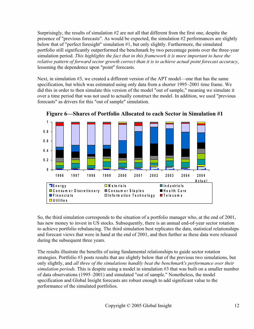
comparing "Sharpe Ratios" (which is a measurement of return per unit of risk) between the portfolio and the benchmark. The Sharpe Ratio is higher (better) for the portfolio when measured on both a three-year basis (our portfolio=0.106 versus S&P500=0.089), and over the whole nine-year period (our portfolio=0.310 versus S&P500=0.283). Furthermore, the results were pretty consistent throughout the simulated period. There was a net "out performance" of the simulated portfolio over the S&P500 for six out of the nine simulated years. As for the other three years, 2000 was the only year of under-performance relative to the S&P500, while the subsequent 2001–02 has both of the simulated portfolios performing roughly the same as the S&P500 benchmark. Thereafter, the out-performance posted by both the simulated portfolios resumes for 2003–04. Figure 5 further highlights the consistent and robust nature of the APT-based portfolio framework. It shows the simulated portfolio outperformed the benchmark on average through a variety of market conditions—this simulation covers a time period when the biggest financial bubble in the history of mankind had occurred. Nonetheless, the model-based framework is robust enough that portfolio results outperformed the S&P500 benchmark on average during years when the benchmark was up, as well as during the years when the benchmark was down. Figure 6 chart shows the optimal sector "weights," or portfolio shares, that were generated by optimizing the APT model-generated expected returns. These are the portfolio allocations that were used in this simulation to achieve the shown portfolio returns. For context, Figure 6 also contains the actual benchmark sector weights that were in place in 2004. The second simulation shown in Figure 4 builds upon the first by using the same APT model to generate expected returns, but here instead of using actual historical data for the forecast drivers, we substitute instead the “old forecasts” that were made by Global Insight at that point in time. This model simulation is still "in-sample," but now we use "previous forecasts" instead of "perfect foresight" actual history. This simulation is only run over 2001–04 due to limitations on the availability of the previous forecasts. The simulation results are overlaid onto the previous simulation results in figure 4 for comparison.
F i g u r e 5 - P e r f o r m a n c e s i n U p a n d D o w n M a r k e t s
- 2 5
- 5
1 5
3 5
U p M a r k e t D o w n M a r k e t
Annu
aliz
ed R
etur
n (%
)
S & P 5 0 0 S im u la t e d P o r t f o l io
Copyright © 2005 Global Insight
12
Surprisingly, the results of simulation #2 are not all that different from the first one, despite the presence of "previous forecasts". As would be expected, the simulation #2 performances are slightly below that of "perfect foresight" simulation #1, but only slightly. Furthermore, the simulated portfolio still significantly outperformed the benchmark by two percentage points over the three-year simulation period. This highlights the fact that in this framework it is more important to have the relative pattern of forward sector growth correct than it is to achieve actual point forecast accuracy, lessening the dependence upon "point" forecasts. Next, in simulation #3, we created a different version of the APT model—one that has the same specification, but which was estimated using only data from a shorter 1995–2001 time frame. We did this in order to then simulate this version of the model "out of sample," meaning we simulate it over a time period that was not used to actually construct the model. In addition, we used "previous forecasts" as drivers for this "out of sample" simulation.
Figure 6—Shares of Portfolio Allocated to each Sector in Simulation #1 So, the third simulation corresponds to the situation of a portfolio manager who, at the end of 2001, has new money to invest in US stocks. Subsequently, there is an annual end-of-year sector rotation to achieve portfolio rebalancing. The third simulation best replicates the data, statistical relationships and forecast views that were in hand at the end of 2001, and then further as these data were released during the subsequent three years. The results illustrate the benefits of using fundamental relationships to guide sector rotation strategies. Portfolio #3 posts results that are slightly below that of the previous two simulations, but only slightly, and all three of the simulations handily beat the benchmark's performance over their simulation periods. This is despite using a model in simulation #3 that was built on a smaller number of data observations (1995–2001) and simulated "out of sample." Nonetheless, the model specification and Global Insight forecasts are robust enough to add significant value to the performance of the simulated portfolios.
0
0 . 2
0 . 4
0 . 6
0 . 8
1
1 9 9 6 1 9 9 7 1 9 9 8 1 9 9 9 2 0 0 0 2 0 0 1 2 0 0 2 2 0 0 3 2 0 0 4 2 0 0 4A c t u a l
E n e r g y M a t e r i a l s I n d u s t r i a l sC o n s u m e r D i s c r e t i o n a r y C o n s u m e r S t a p l e s H e a l t h C a r eF i n a n c i a l s I n f o r m a t i o n T e c h n o l o g y T e l e c o m sU t i l i t i e s

Copyright © 2005 Global Insight
13
The cumulative out performance shown in Figure 4 occurs rather consistently throughout the simulation period under a variety of conditions and assumptions. Of course, counterfactual simulations are artificial by their nature. For example, few would allow the strategic management of their portfolios be turned over completely to a mechanical framework, despite the historical validity. Also, this model only speaks to sector-level exposure, and from a strategic, not tactical, perspective. When taking company-level exposure in a portfolio there is obviously additional analysis required, such as management performance and balance sheet positions. Further, a large body of research and common experience have shown that it is just as important, for consistent out performance, to respect technical conditions present in the market in addition to fundamental relationships. Still, with those caveats, these simulations clearly demonstrate that this fundamentally based APT framework has value and can help construct portfolios and set sector rotation strategies. The tool aids in understanding current and historical market performances, and providing a robust basis for generating expected returns and the optimal portfolio composition. Conclusion We have presented a practical APT model framework for forecasting total returns in stock market sectors. This framework was created from the latest available research, data observations, and sector classification conventions that are commonly used in portfolio management. The model was constructed with attributes that add significant value to the process of sector-based portfolio management. In addition, the APT framework helps investors determine which market forces are predominant at different points in time, and why that is so. The framework presented here does not depend very crucially upon the forecast model drivers. Most of the relationships are with leading indicators. Still, clear forward links with the macro economy do allow analysts and portfolio managers to simulate their own macroeconomic views, derive the consequent settings for interest rates and the distribution of growth rates in sector profits, and then use this framework to calculate the likely impact on portfolio performances. As a result, this framework provides a solid and clear basis for achieving higher portfolio returns over the medium and long term, without taking on significant additional risk, through a sector-based portfolio rotation strategy. Left for further research is the effort to extend this framework to include Europe, Japan, and other major stock markets around the world.

Copyright © 2005 Global Insight
14
Appendix 1—Theoretical Background of APT Models The Arbitrage Pricing Theory (APT) was introduced by Ross in 1976 and extended by Huberman5, Chamberlain and Rothschild6. It grew out of empirical work that was founded upon the classic Capital Asset Pricing Model (CAPM). For the past four decades, the CAPM developed by Sharpe7, Lintner8 and Mossin9 has served as a cornerstone of financial theory. One of the main goals of financial research during this time has been to extend the basic CAPM to make it more theoretically complete and empirically accurate. However, CAPM models typically do not fit the empirical facts very well. For example, Gibbons10, MacKinlay11, Reinganum12, Lakonishok and Shapiro13, and Coggin and Hunter14 could not find strong evidence for the CAPM expected return-market beta relation. Nor were Fama and French 15 able to find statistically significant relation between beta and expected return, yet they found evidence of significant effects on asset returns due to some other factors, such as size and book-to-market ratio. These were the landmark results that eventually supported the argument that the Market Portfolio as the only risk source is not capable of adequately explaining actual returns. As a result, there have been theoretical attempts to extend the conceptual foundation of the CAPM such as in the Intertemporal Capital Asset Pricing Model (Merton16), Arbitrage Pricing Theory (Ross17), and Consumption Capital Asset Pricing Model (Breeden18, Grossman and Shiller19). Extending further, Campbell20 substitutes asset returns and returns on human capital for consumption. Hansen and Singleton21 developed the analysis in terms of the stochastic discount factor. More recently, relatively exotic utility functions have been proposed to explain such anomalies as the equity premium puzzle, Campbell and Cochrane22, Constantinidies and Duffie23. A more limited approach with the same objective has been to develop conditional CAPMs that allow betas to change over time as in Harvey24 and Jagannathan and Wang25. The dissatisfaction with empirical results of these CAPM models led to the creation of the APT model, with its multifactor structure. This approach is sometimes called the "raw empiricism” approach to filling the gaps for the poor CAPM empirical results. The APT structure allows the model to take into account a larger number of "beta" parameters, each of them representing asset sensitivity to a different particular factor. According to the APT equation, asset value fluctuation is influenced not only by a total market factor (market portfolio value), but by other economic factors as well, including non-market risk factors such as national currency exchange rates, energy prices, inflation and unemployment rates, etc. Taking several factors into account gives a more precise model for forecasting changes in asset prices, and reduction of non-systematic risk. The APT model depends on the law of one price and categorizes the risk of an asset into two parts: systematic risk, which is a result of more than one common factor, and unsystematic risk. Thus, in the APT framework there is a linear relation between the expected return and “k“ number of common factor betas that is proposed under the assumptions of homogeneous investor expectations, risk averse utility maximizing investors, a frictionless and perfectly competitive capital market with no asymptotic arbitrage opportunities. As opposed to the one factor framework of CAPM, APT employs k factors in the pricing relation.

Copyright © 2005 Global Insight
15
Then, the next theoretical question is "which economic factors have significant effects on the pricing mechanism"? Some macroeconomic changes are shown to affect asset prices stronger than others, while some do not seem to affect them at all. One of the most famous APT tests on this subject was implemented by Chen, Roll and Ross, 26 who considered whether several macroeconomic variables have systematic influence on asset returns. They found there are several that do, including: the spread between long- and short-term interest rates, the difference between expected and unexpected inflation, the growth of industrial production, and the spread between high- and low-grade bonds. Other empirical APT studies only focused on determining the number of risk factors that systematically explain the stock market returns by implementing Factor Analysis Methods. For example, Roll and Ross27 found that three or four systematic risk factors are statistically adequate to explain asset returns over 1962–72, while Chen28 found five factors affecting results from the NYSE and AMEX during 1963–78. Dhrymes et.al29 found that the number of factors that give best results actually changed depending on the period length and the size of the stock groups under analysis. One drawback to this approach is, although the number of factors can be estimated, the identification of which factors actually determine a stock price is not possible. In recent years, other empirical work in macroeconomics and finance has suggested that aggregate movements in financial constraints, monetary and credit conditions or business cycles might affect the firm value and thus total return. Cochrane30 showed how the investment-capital ratio predicts returns; Lettau & Ludvigson31 showed that an estimated consumption-wealth ratio predicts returns; and Santos & Veronesi32 showed that the consumption-labor income ratio predicts returns. Also, numerous studies have shown that it is possible to track the time variation in expected returns using financial ratios, such as the price-dividend ratio and the dividend yield (e.g. Fama and French33), the price-earnings ratio and the ratio of current earnings to an average of previous earnings (Campbell and Shiller34), the dividend-earnings ratio (Lamont35), and the ratio of a short-term interest rate to its historic moving average (Campbell36 and Hodrick37). Lamont, Polk, etc38 studied if the impact of financial constraints on firm value is observable in stock returns. They showed that financially constrained firm’s stock returns move together over time suggesting that constrained firms are subject to common shocks. They also found no evidence that the relative performance of constrained firms reflects monetary policy, credit conditions, or business cycles, instead being seemingly more related to earnings growth and spending requirements, as highlighted by growth of free cash flow. Stock and Watson39 showed that the yield curve, in the form of interest rate spreads, does well in forecasting both economic output patterns and asset returns. Also, according to Kleim and Stambaugh40, the yield curve may be a robust measure the state of monetary policy, credit conditions and growth expectations.

Copyright © 2005 Global Insight
16
Appendix 2 - Data Sources, Transformations, and Descriptive Statistics Table 1 lists the Data Sources for each of the indicators used in the APT model, and describes the transformations or data extensions used to put the variables into the model format. A full set of these data are available to clients of Global Insight upon request.
Table 1 Variable Name
Source of Data Data Series Mnemonics Notes
1. Total Return
S&P TOTAL RETURN INDEX, INDEX BASE: 30 DEC 1994 = 100 (source: STANDARD AND POOR'S CORPORATION, S&P ANALYSTS' HANDBOOK)
SANDP: TRIENSECNS.Q, SANDP:TRIMATSECNS.Q, SANDP:TRIINDUSSECNS.Q, SANDP:TRICONDISSECNS.Q, SANDP:TRICONSTPSECNS.Q, SANDP:TRIHLTHSECNS.Q, SANDP:TRIITSECNS.Q, SANDP:TRIFINSECNS.Q, SANDP:TRITELSERSECNS.Q, SANDP:TRIUTILSECNS.Q
Total return data for 10 GICS economic sectors retrieved from SANDP databank are available starting Q31998. Further history was extended backwards in time using the growth rates of total return of the corresponding sectors previously specified in SIC terms.
2. Three month T-Bill Rate
Global Insight's U.S. Macro Economic Forecast Data Bank
USMACRO_TR25:RMTB3M.Q USMACRO_TR25:RMTB3M.Q
Note - Subtracting the compound return from the (risk-free) 3-month T-Bill from the Total Return for each sector means we are specifying the Left Hand Side variable as the "Excess Returns" earned over and above that obtained by simply buying the risk free rate, in line with the theoretical and practical model structure.
Calculations: Compounding formula: (1+3mtb [-3]/400)*(1+3mtb [-2]//400)*(1+3mtb [-1]/400)*(1+3mtb/400) 3. Dividend payout ratio
DIVIDENDS: S&P: DPS, PER SHARE DATA, STANDARD AND POOR'S CORPORATION, S&P ANALYSTS' HANDBOOK EARNINGS S&P: DILUTED EPS, PER SHARE DATA STANDARD AND POOR'S CORPORATION S&P ANALYSTS' HANDBOOK
DIVIDENDS: SANDP: DIVENSECNS.Q, SANDP: DIVMATSECNS.Q, SANDP: DIVINDUSSECNS.Q, SANDP: DIVCONDISSECNS.Q, SANDP: DIVCONSTPSECNS.Q, SANDP: DIVHLTHSECNS.Q, SANDP: DIVITSECNS.Q, SANDP: DIVFINSECNS.Q, SANDP: DIVTELSERSECNS.Q, SANDP: DIVUTILSECNS.Q EARNINGS EARNENSECNS.Q, SANDP: EARNMATSECNS.Q, SANDP: EARNINDUSSECNS.Q SANDP: EARNCONDISSECNS.Q, SANDP: EARNCONSTPSECNS.Q, SANDP: EARNHLTHSECNS.Q, SANDP: EARNITSECNS.Q, SANDP: EARNFINSECNS.Q, SANDP: EARNTELSERSECNS.Q, SANDP: EARNUTILSECNS.Q
Dividend Payout ratio defined as sum of the four quarter dividends divided by the sum of the four quarter earnings.
Dividends and Earnings data for 10 GICS economic sectors retrieved from SANDP databank are available starting Q31998. Further history was extended backwards in time using the growth rates of the dividends and earnings of the corresponding sectors previously specified in SIC terms.
Calculations: Growth of the dividend payout ratio formula is:
DE[-5])/3:]SUM(DE[-15DE[-3]):SUM(DE
=rowthyoutRatioGDividendPa , where DE=Dividends/Earnings
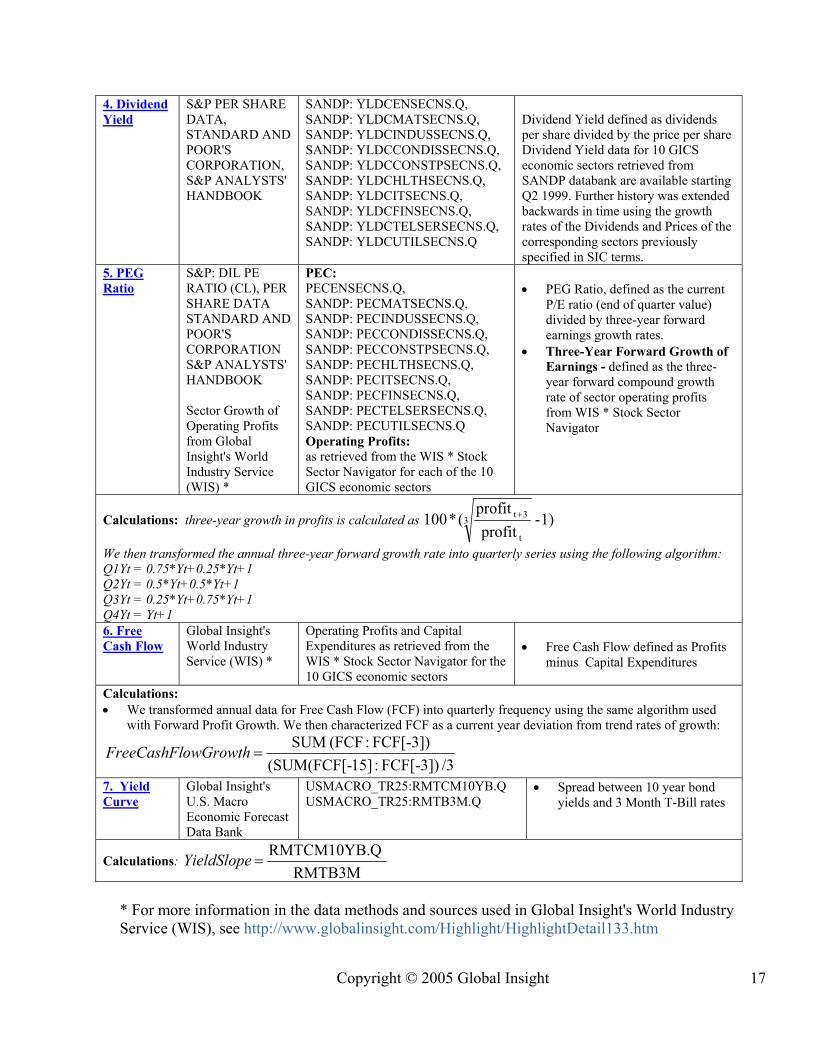
Copyright © 2005 Global Insight
17
4. Dividend Yield
S&P PER SHARE DATA, STANDARD AND POOR'S CORPORATION, S&P ANALYSTS' HANDBOOK
SANDP: YLDCENSECNS.Q, SANDP: YLDCMATSECNS.Q, SANDP: YLDCINDUSSECNS.Q, SANDP: YLDCCONDISSECNS.Q, SANDP: YLDCCONSTPSECNS.Q, SANDP: YLDCHLTHSECNS.Q, SANDP: YLDCITSECNS.Q, SANDP: YLDCFINSECNS.Q, SANDP: YLDCTELSERSECNS.Q, SANDP: YLDCUTILSECNS.Q
Dividend Yield defined as dividends per share divided by the price per share Dividend Yield data for 10 GICS economic sectors retrieved from SANDP databank are available starting Q2 1999. Further history was extended backwards in time using the growth rates of the Dividends and Prices of the corresponding sectors previously specified in SIC terms.
5. PEG Ratio
S&P: DIL PE RATIO (CL), PER SHARE DATA STANDARD AND POOR'S CORPORATION S&P ANALYSTS' HANDBOOK Sector Growth of Operating Profits from Global Insight's World Industry Service (WIS) *
PEC: PECENSECNS.Q, SANDP: PECMATSECNS.Q, SANDP: PECINDUSSECNS.Q, SANDP: PECCONDISSECNS.Q, SANDP: PECCONSTPSECNS.Q, SANDP: PECHLTHSECNS.Q, SANDP: PECITSECNS.Q, SANDP: PECFINSECNS.Q, SANDP: PECTELSERSECNS.Q, SANDP: PECUTILSECNS.Q Operating Profits: as retrieved from the WIS * Stock Sector Navigator for each of the 10 GICS economic sectors
• PEG Ratio, defined as the current
P/E ratio (end of quarter value) divided by three-year forward earnings growth rates.
• Three-Year Forward Growth of Earnings - defined as the three-year forward compound growth rate of sector operating profits from WIS * Stock Sector Navigator
Calculations: three-year growth in profits is calculated as 1)-profit
profit(*100 3
t
3t+
We then transformed the annual three-year forward growth rate into quarterly series using the following algorithm: Q1Yt = 0.75*Yt+0.25*Yt+1 Q2Yt = 0.5*Yt+0.5*Yt+1 Q3Yt = 0.25*Yt+0.75*Yt+1 Q4Yt = Yt+1 6. Free Cash Flow
Global Insight's World Industry Service (WIS) *
Operating Profits and Capital Expenditures as retrieved from the WIS * Stock Sector Navigator for the 10 GICS economic sectors
• Free Cash Flow defined as Profits
minus Capital Expenditures
Calculations: • We transformed annual data for Free Cash Flow (FCF) into quarterly frequency using the same algorithm used
with Forward Profit Growth. We then characterized FCF as a current year deviation from trend rates of growth:
/3FCF[-3]):15](SUM(FCF[-FCF[-3]):(FCF SUM
=owGrowthFreeCashFl
7. Yield Curve
Global Insight's U.S. Macro Economic Forecast Data Bank
USMACRO_TR25:RMTCM10YB.Q USMACRO_TR25:RMTB3M.Q
• Spread between 10 year bond yields and 3 Month T-Bill rates
Calculations: RMTB3M
QRMTCM10YB.=YieldSlope
* For more information in the data methods and sources used in Global Insight's World Industry Service (WIS), see http://www.globalinsight.com/Highlight/HighlightDetail133.htm
Copyright © 2005 Global Insight
18
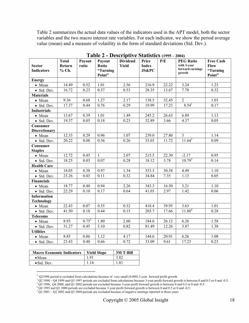
Table 2 summarizes the actual data values of the indicators used in the APT model, both the sector variables and the two macro interest rate variables. For each indicator, we show the period average value (mean) and a measure of volatility in the form of standard deviations (Std. Dev.).
Table 2 - Descriptive Statistics (1995 – 2004) Sector Indicators
Total Return % Ch.
Payout ratio
Payout Ratio “Turning Point”
Dividend Yield
Price Index JS&PC
P/E PEG Ratio with 3-year forward earnings growth
Free Cash Flow “Turning Point”
Energy • Mean 14.49 0.52 1.01 2.56 216.9 22.22 3.24 1.23 • Std. Dev. 16.72 0.23 0.57 0.53 28.35 13.67 7.78 0.32
Materials • Mean 9.36 0.68 1.27 2.17 138.5 32.45 2 1.03 • Std. Dev. 17.37 0.44 0.76 0.29 19.99 17.23 8.541 0.17
Industrials • Mean 13.67 0.39 1.01 1.49 245.2 26.63 6.89 1.13 • Std. Dev. 19.37 0.05 0.18 0.23 32.89 3.66 4.37 0.05
Consumer Discretionary
• Mean 12.33 0.29 0.96 1.07 239.0 27.80 3 1.14 • Std. Dev. 20.22 0.08 0.36 0.26 33.03 11.72 11.642 0.09
Consumer Staples
• Mean 12.72 0.45 1 2.07 215.5 22.30 -2.17 0.95 • Std. Dev. 18.25 0.03 0.07 0.28 18.12 3.78 10.793 0.14
Health Care • Mean 18.05 0.38 0.97 1.34 353.3 30.58 4.49 1.10 • Std. Dev. 23.26 0.03 0.11 0.32 34.84 7.35 1.13 0.05
Financials • Mean 18.77 0.40 0.94 2.26 343.3 16.50 3.21 1.10 • Std. Dev. 22.29 0.10 0.17 0.64 41.03 2.97 1.42 0.06
Information Technology
• Mean 22.43 0.07 0.55 0.32 418.4 39.95 3.63 1.01 • Std. Dev. 41.50 0.18 0.44 0.15 203.7 17.66 11.804 0.28
Telecoms • Mean 8.93 0.755 1.80 2.60 184.6 26.12 6.26 1.58 • Std. Dev. 31.27 0.45 3.10 0.82 81.49 12.26 3.87 1.38
Utilities • Mean 8.85 0.86 1.12 4.17 144.6 20.91 6.26 1.08 • Std. Dev. 23.43 0.40 0.66 0.72 33.09 9.61 17.23 0.23
Macro Economic Indicators Yield Slope 3M T-Bill • Mean 1.91 3.82 • Std. Dev. 1.14 1.81
1 Q21996 period is excluded from calculations because of very small (0.098) 3-year forward profit growth 2 Q2 1998 – Q4 1999 and Q3 1997 periods are excluded from calculations because 3-year profit forward growth is between 0 and 0.5 or 0 and -0.5. 3 Q3 1996, Q4 2000, and Q1 2002 periods are excluded because 3-year profit forward growth is between 0 and 0.5 or 0 and -0.5. 4 Q4 1995 and Q1 2000 periods are excluded because 3-year profit forward growth is between 0 and 0.5 or 0 and -0.5. 5 Q2 2001 – Q2 2002 and Q3 2004 periods are excluded because of negative earnings reported in those years

Copyright © 2005 Global Insight
19
Footnotes and References: 1 For the description of GICS see: http://www2.standardandpoors.com/servlet/Satellite?pagename=sp/sp_product/UmbrellaBodyTemplate&cid=1021984026045&l=EN&s=&b=11&f=1&r=1&ig= 2 Hirst, D.E., and P.E. Hopkins, 2000, "Earnings: Measurement, Disclosure, and the Impact on Equity Valuation." Monograph for the Research Foundation of the Institute of Chartered Financial Analysts and the Association for Investment Management and Research, Charlottesville, VA 3 For more information on Global Insight's World Industry Service (WIS), see: http://www.globalinsight.com/Highlight/HighlightDetail133.htm 4 Hecht P. and T. Vuolteenaho "Explaining Returns with Cash-Flow Proxies", draft dated 26-Oct-2004 5 Huberman, Gur, 1982, "A Simple Approach to Arbitrage Pricing Theory", Journal of Economic Theory, 28, 183–191 6 Chamberlain, G., and M. Rothschild, 1983, “Arbitrage, Factor Structure, and Mean Variance Analysis on Large Asset Markets,” Econometrica, 52, 1281–1304. 7 Sharpe, W. F., 1964, “Capital Asset Prices: A Theory of Market Equilibrium under Conditions of Risk,” Journal of Finance, 19, 425–442. 8 Lintner, J., 1965, “The Valuation of Risk Assets and the Selection of Risky Investments in Stock Portfolios and Capital Budgets,” Review of Economics and Statistics, 47, 13–37. 9 Mossin J., 1966. "Equilibrium in a capital asset market", Econometrica, 34:768-783. 10 Gibbons, M. R., 1982, “Multivariate Tests of Financial Models: A New Approach,” Journal of Financial Economics, 10, 3–27. 11 MacKinlay, A. C., 1987, "On Multivariate Tests of the CAPM," Journal of Financial Economics, 18, 341-372. 12 Reinganum, M., 1981 "Misspecification of capital asset pricing: Empirical anomalies", Journal of Financial Economics, 9, 19-46. 13 Lakonishok, J. and C.Shapiro, 1986, "Systematic risk, total risk and size determinants of stock market returns", Journal of Banking and Finance 10, 115 - 132. 14 Coggin, T.D. and J.E.Hunter (1985), “Are High-Beta, Large Capitalization Stocks Overpriced?”, Financial Analysts Journal, Vol.41, 70-71. 15 Fama, E. and K. French, 1992, "The cross-section of expected stocks returns", Journal of Finance 67, 427– 465. 16 Merton, R.C., 1973, An intertemporal capital asset-pricing model, Econometrica, 41 (4), 867-887. 17Ross, S. A., 1976, "The Arbitrage Theory of Capital Asset Pricing" Journal of Economic Theory, 13, 341-360. 18 Breeden, Douglas T., 1979, An intertemporal asset-pricing model with stochastic consumption and investment opportunities, Journal of Financial Economics, 7 (4), 265-96. 19 Grossman, Sanford J. and Shiller, Robert J., 1981, The determinants of the variability of stock market prices, A.E.R. Papers and Proc., 71 (3), 222-27. 20 Campbell, J. Y., 1996, Understanding risk and return, Journal of Political Economy, 104 (2), 298-345. 21 Hansen, Lars P. and Singleton, Kenneth J., 1983, Stochastic consumption, risk aversion, and the temporal behavior of asset returns, Journal of Political Economy, 91 (2), 249-65. 22 Campbell, John Y. and John H. Cochrane, 1999, By force of habit: A consumption-based explanation of aggregate stock market behavior, Journal of Political Economy, 107 (2), 205-251. 23 Constantinidies, George M. and Darrell Duffie, 1996, Asset pricing with heterogeneous consumers, Journal of Political Economy, 104 (2), 219-240 24 Harvey, Campbell R. 1989, Time-varying conditional covariances in tests of asset-pricing models, Journal of Financial Economics, 24 (2), 289-318 25 Jagannathan, Ravi and Zhenyu Wang, 1996, The conditional CAPM and the cross-section of stock returns, Journal of Finance, 51 (1), 3-53 26 Chen N, Roll R and Ross SA. 1986, "Economic forces and the stock market", Journal of Business, 59:383-403. 27 Roll, R. W., and S. A. Ross, 1980, “An Empirical Investigation of the Arbitrage Pricing Theory,” Journal of Finance, 35, 1073–1103. 28 Chen, N., 1983, “Some Empirical Tests of the Theory of Arbitrage Pricing,” Journal of Finance, 38, 1393–1414. 29 Dhrymes, Phoebe, Irwin Friend, and Mustafa Gultekin, 1984, "A Critical Re-Examination of the Empirical Evidence on the Arbitrage Pricing Theory", Journal of Finance, 39(2), 323–346. 30 Cochrane, John H., 1991, "Production-Based Asset Pricing and the Link Between Stock Returns and Economic Fluctuations", Journal of Finance 46(1), 209-37.

Copyright © 2005 Global Insight
20
31 Lettau, M., and S. Ludvigson (2001a): “Consumption, Aggregate Wealth and Expected Stock Returns,” Journal of Finance, 56(3), 815–849; (2001b): “Resurrecting the CAPM: A Cross-Sectional Test when Risk Premia are Time-Varying”, Journal of Political Economy 109(6), 1238– 1287. 32 Santos, J., and P. Veronesi (2000), "Labor Income & Predictable Stock Returns", Unpubl, U. of Chicago. 33 Fama, E. F., and K. R. French (1988a), "Dividend Yields and Expected Stock Returns", Journal of Financial Economics, 22, 3. (1988b), "Permanent and Temporary Components of Stock Prices", Journal of Political Economy, 96(2), 246.273. (1989), "Business Conditions and Expected Returns on Stocks and Bonds", Journal of Financial Economics 25, 23-49. 34 Campbell, J. Y., and R. J. Shiller (1988), "The Dividend-Price Ratio and Expectations of Future Dividends and Discount Factors", Review of Financial Studies 1, 195-227. 35 Lamont O.(1998) "Earnings and expected returns" Journal of Finance 53, 5, 1563-1587. 36 Campbell, J. (1991), "A Variance Decomposition for Stock Returns", Economic Journal 101, 157-179. 37 Hodrick, R. (1992), "Dividend Yields and Expected Stock Returns: Alternative Procedures for Inference and Measurement", Review of Financial Studies 5, 357-386. 38 Lamont, Owen, Christopher Polk and Jesus Saa-Requejo, (2001), "Financial Constraints and Stock Returns", forthcoming, Review of Financial Studies. 39 Stock, J.H. and M.W. Watson (1989), "New indexes of coincident and leading economic indicators", NBER Macroeconomic Annual, 351-393 40 Stambaugh, R.,1986, "Bias in Regressions with Lagged Stochastic Regressors", Unpubl., U. of Chicago.
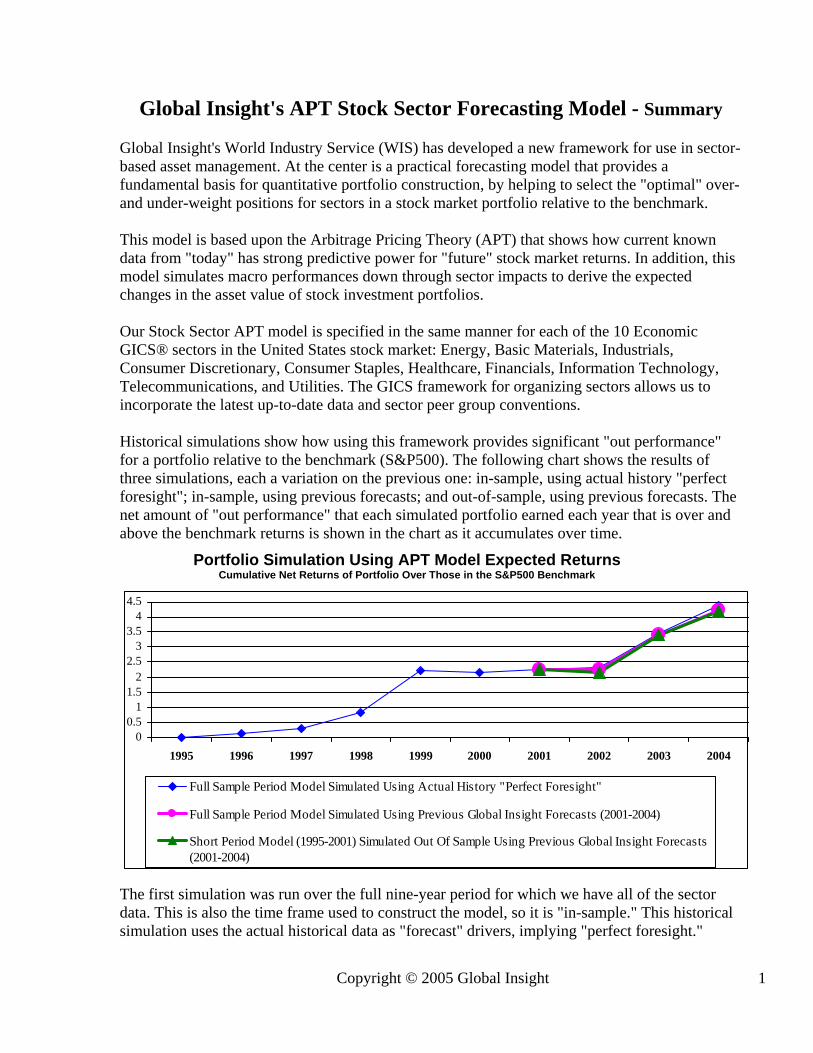
Global Insight's APT Stock Sector Forecasting Model - Summary Global Insight's World Industry Service (WIS) has developed a new framework for use in sector-based asset management. At the center is a practical forecasting model that provides a fundamental basis for quantitative portfolio construction, by helping to select the "optimal" over- and under-weight positions for sectors in a stock market portfolio relative to the benchmark. This model is based upon the Arbitrage Pricing Theory (APT) that shows how current known data from "today" has strong predictive power for "future" stock market returns. In addition, this model simulates macro performances down through sector impacts to derive the expected changes in the asset value of stock investment portfolios. Our Stock Sector APT model is specified in the same manner for each of the 10 Economic GICS® sectors in the United States stock market: Energy, Basic Materials, Industrials, Consumer Discretionary, Consumer Staples, Healthcare, Financials, Information Technology, Telecommunications, and Utilities. The GICS framework for organizing sectors allows us to incorporate the latest up-to-date data and sector peer group conventions. Historical simulations show how using this framework provides significant "out performance" for a portfolio relative to the benchmark (S&P500). The following chart shows the results of three simulations, each a variation on the previous one: in-sample, using actual history "perfect foresight"; in-sample, using previous forecasts; and out-of-sample, using previous forecasts. The net amount of "out performance" that each simulated portfolio earned each year that is over and above the benchmark returns is shown in the chart as it accumulates over time. Portfolio Simulation Using APT Model Expected Returns
Cumulative Net Returns of Portfolio Over Those in the S&P500 Benchmark
00.5
11.5
22.5
33.5
44.5
1995 1996 1997 1998 1999 2000 2001 2002 2003 2004
Full Sample Period Model Simulated Using Actual History "Perfect Foresight"
Full Sample Period Model Simulated Using Previous Global Insight Forecasts (2001-2004)
Short Period Model (1995-2001) Simulated Out Of Sample Using Previous Global Insight Forecasts(2001-2004)
The first simulation was run over the full nine-year period for which we have all of the sector data. This is also the time frame used to construct the model, so it is "in-sample." This historical simulation uses the actual historical data as "forecast" drivers, implying "perfect foresight."
Copyright © 2005 Global Insight
1
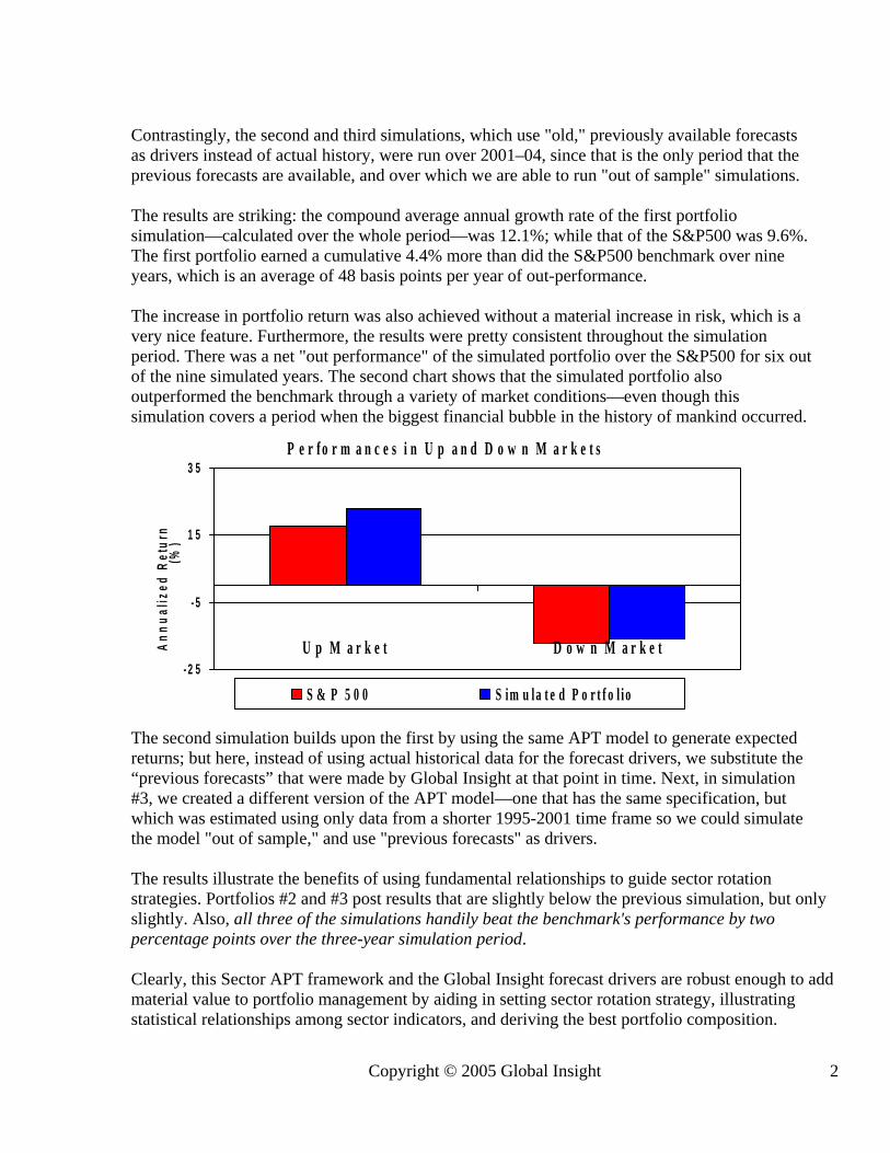
Contrastingly, the second and third simulations, which use "old," previously available forecasts as drivers instead of actual history, were run over 2001–04, since that is the only period that the previous forecasts are available, and over which we are able to run "out of sample" simulations. The results are striking: the compound average annual growth rate of the first portfolio simulation—calculated over the whole period—was 12.1%; while that of the S&P500 was 9.6%. The first portfolio earned a cumulative 4.4% more than did the S&P500 benchmark over nine years, which is an average of 48 basis points per year of out-performance. The increase in portfolio return was also achieved without a material increase in risk, which is a very nice feature. Furthermore, the results were pretty consistent throughout the simulation period. There was a net "out performance" of the simulated portfolio over the S&P500 for six out of the nine simulated years. The second chart shows that the simulated portfolio also outperformed the benchmark through a variety of market conditions—even though this simulation covers a period when the biggest financial bubble in the history of mankind occurred.
P e r f o r m a n c e s i n U p a n d D o w n M a r k e t s
- 2 5
- 5
1 5
3 5
U p M a r k e t D o w n M a r k e tAnnu
aliz
ed R
etur
n (%
)
S & P 5 0 0 S im u la t e d P o r t f o l io
The second simulation builds upon the first by using the same APT model to generate expected returns; but here, instead of using actual historical data for the forecast drivers, we substitute the “previous forecasts” that were made by Global Insight at that point in time. Next, in simulation #3, we created a different version of the APT model—one that has the same specification, but which was estimated using only data from a shorter 1995-2001 time frame so we could simulate the model "out of sample," and use "previous forecasts" as drivers. The results illustrate the benefits of using fundamental relationships to guide sector rotation strategies. Portfolios #2 and #3 post results that are slightly below the previous simulation, but only slightly. Also, all three of the simulations handily beat the benchmark's performance by two percentage points over the three-year simulation period. Clearly, this Sector APT framework and the Global Insight forecast drivers are robust enough to add material value to portfolio management by aiding in setting sector rotation strategy, illustrating statistical relationships among sector indicators, and deriving the best portfolio composition.
Copyright © 2005 Global Insight
2