global routing. global routing: sequential −one net at a time concurrent −order-independent...
TRANSCRIPT

Global Routing
Global Routing
• Global routing:
Sequential− One net at a time
Concurrent− Order-independent− ILP
2
3
Integer Linear Programming
• A linear program (LP) consists of a set of constraints and an optional objective function
• Objective function is maximized or minimized
• Both the constraints and the objective function must be linear
Constraints form a system of linear equations and inequalities
4
Routing by Integer Linear Programming
• Integer linear program (ILP): Every variable can only assume integer values
Typically takes much longer to solve In many cases, variables are only allowed to be 0 or 1
• ILP solvers: GLPK CPLEX MOSEK

5
Routing by ILP• Inputs:
W × H routing grid G Routing edge capacities Netlist
• Two sets of variables k Boolean variables for each net net:
− xnet1, xnet2, … , xnetk
− xneti= 1 path i is selected for net k real variables for each net net:
− wnet1, wnet2, … , wnetk
− wneti = desirability of path i for net (e.g., less bends = larger w)
6
Routing by ILP• Two types of constraints
Uniqueness:
− Each net must select a single route (mutual exclusion)
Edge capacities
7
Routing by ILP
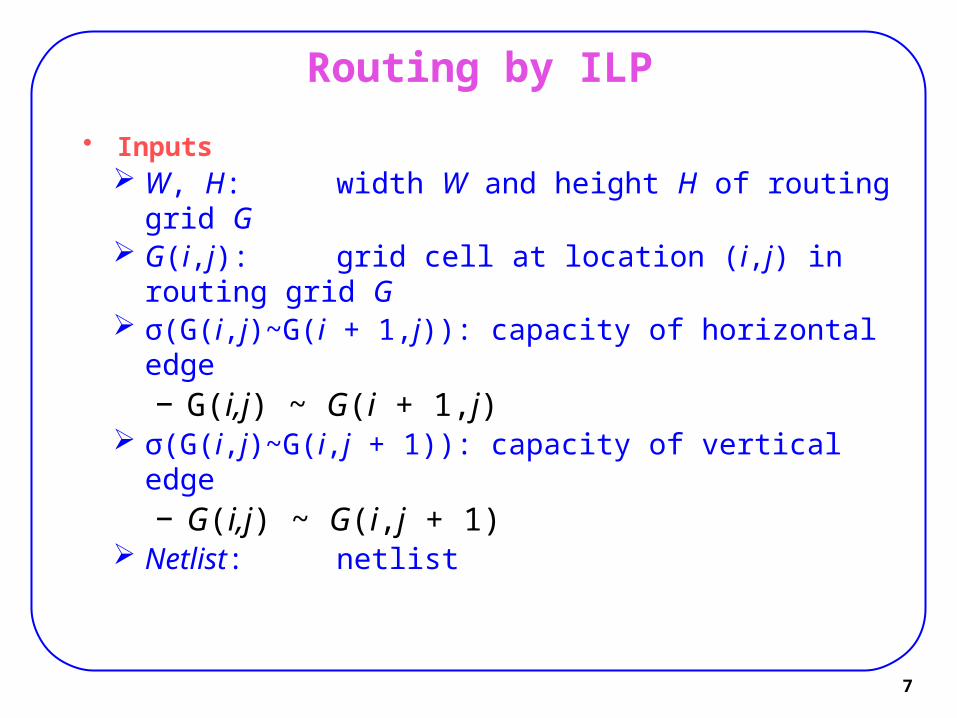
• Inputs W, H: width W and height H of routing grid G G(i,j): grid cell at location (i,j) in routing grid G σ(G(i,j)~G(i + 1,j)): capacity of horizontal edge
− G(i,j) ~ G(i + 1,j) σ(G(i,j)~G(i,j + 1)): capacity of vertical edge
− G(i,j) ~ G(i,j + 1) Netlist: netlist
8
Routing by ILP
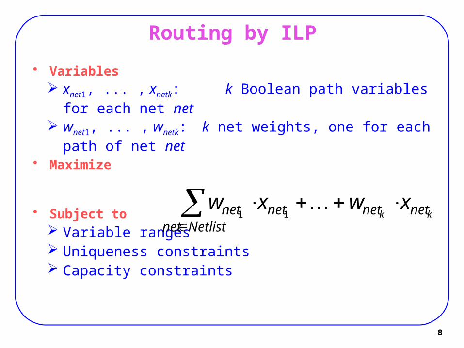
• Variables xnet1, ... , xnetk: k Boolean path variables for each net
net wnet1, ... , wnetk: k net weights, one for each path of net net
• Maximize
• Subject to Variable ranges Uniqueness constraints Capacity constraints
Netlistnet
netnetnetnet kkxwxw
11
9
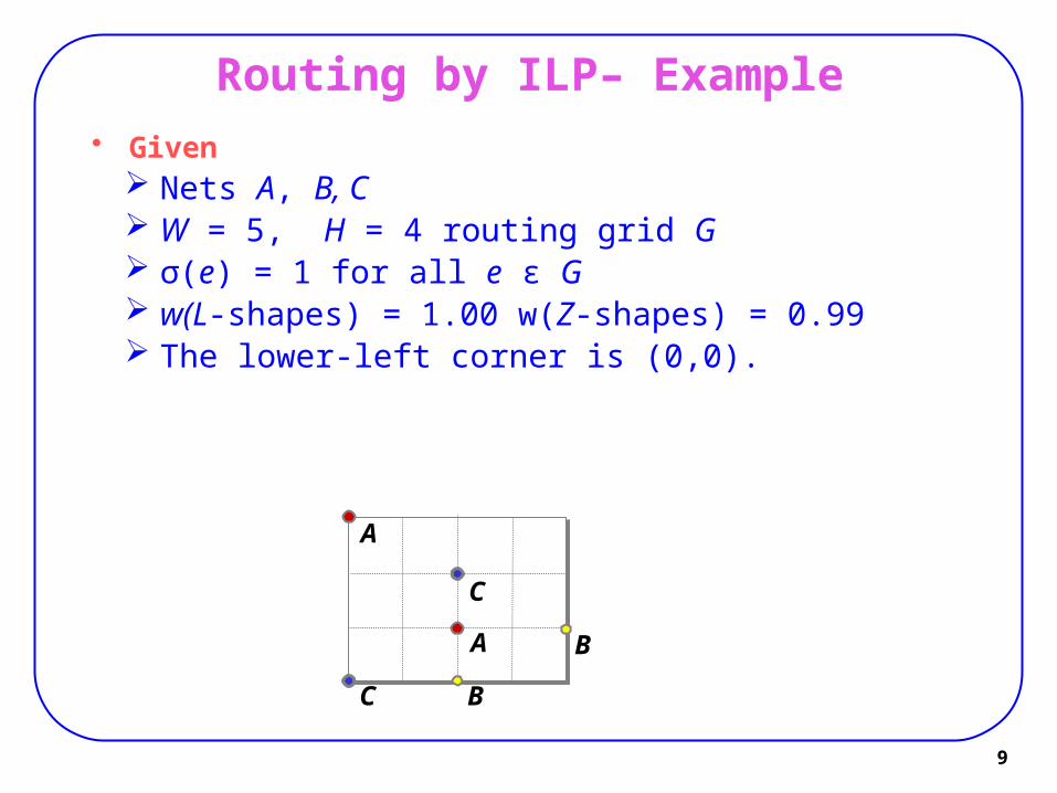
Routing by ILP– Example• Given
Nets A, B, C W = 5, H = 4 routing grid G σ(e) = 1 for all e ϵ G w(L-shapes) = 1.00 w(Z-shapes) = 0.99 The lower-left corner is (0,0).
A
A B
BC
C

10
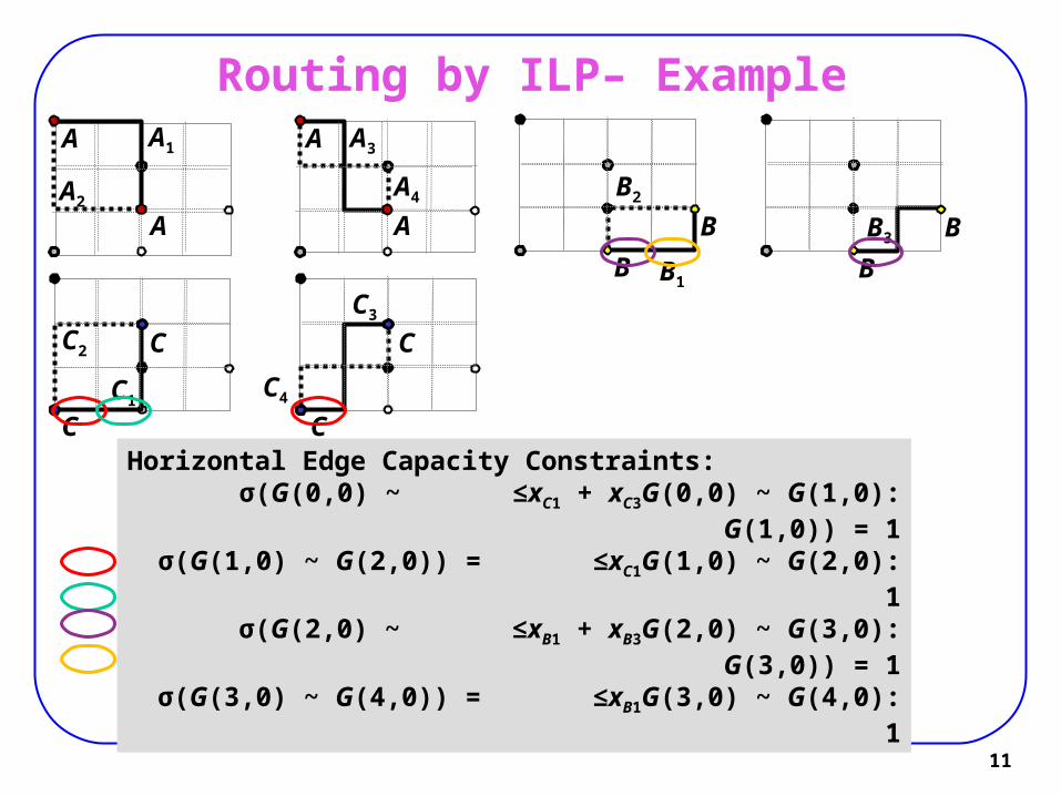
Routing by ILP– ExampleFor net A, possible routes: two L-shapes (A1,A2) and two Z-shapes (A3,A4)
Net Constraints:xA1 + xA2 + xA3 + xA4 ≤ 1Variable Constraints:0 ≤ xA1 ≤ 1, 0 ≤ xA2 ≤ 1,
0 ≤ xA3 ≤ 1, 0 ≤ xA4 ≤ 1
A
AA2
A1 A
A
A4
A3
Net Constraints:xB1 + xB2 + xB3 ≤ 1Variable Constraints:0 ≤ xB1 ≤ 1, 0 ≤ xB2 ≤ 1,
0 ≤ xB3 ≤ 1 B
B B1
B2
B3 B
B
Net Constraints:xC1 + xC2+ xC3 + xC4 ≤ 1Variable Constraints:0 ≤ xC1 ≤ 1, 0 ≤ xC2 ≤ 1,
0 ≤ xC3 ≤ 1, 0 ≤ xC4 ≤ 1 C
C
C
CC2
C1
C3
C4
For net B, the possible routes: two L-shapes (B1,B2) and one Z-shape (B3)
For net C, the possible routes: two L-shapes (C1,C2) and two Z-shapes (C3,C4)
11
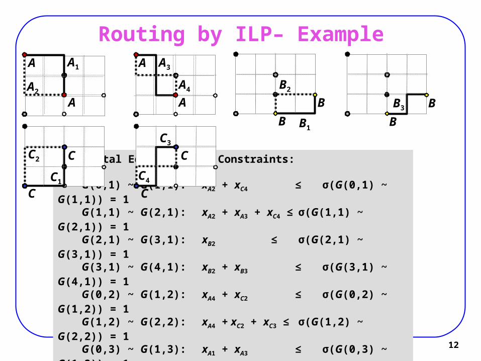
Routing by ILP– Example
Horizontal Edge Capacity Constraints:G(0,0) ~ G(1,0):xC1 + xC3 ≤σ(G(0,0) ~ G(1,0)) = 1G(1,0) ~ G(2,0):xC1 ≤σ(G(1,0) ~ G(2,0)) = 1G(2,0) ~ G(3,0):xB1 + xB3 ≤σ(G(2,0) ~ G(3,0)) = 1G(3,0) ~ G(4,0):xB1 ≤σ(G(3,0) ~ G(4,0)) = 1
A
AA2
A1 A
A
A4
A3
B
B B1
B2
B3 B
B
C
C
C
CC2
C1
C3
C4
12
Routing by ILP– Example
Horizontal Edge Capacity Constraints:
G(0,1) ~ G(1,1): xA2 + xC4 ≤ σ(G(0,1) ~ G(1,1)) = 1G(1,1) ~ G(2,1): xA2 + xA3 + xC4 ≤ σ(G(1,1) ~ G(2,1)) = 1G(2,1) ~ G(3,1): xB2 ≤ σ(G(2,1) ~ G(3,1)) = 1G(3,1) ~ G(4,1): xB2 + xB3 ≤ σ(G(3,1) ~ G(4,1)) = 1
G(0,2) ~ G(1,2): xA4 + xC2 ≤ σ(G(0,2) ~ G(1,2)) = 1G(1,2) ~ G(2,2): xA4 + xC2 + xC3 ≤ σ(G(1,2) ~ G(2,2)) = 1G(0,3) ~ G(1,3): xA1 + xA3 ≤ σ(G(0,3) ~ G(1,3)) = 1G(1,3) ~ G(2,3): xA1 ≤ σ(G(1,3) ~ G(2,3)) = 1
A
AA2
A1 A
A
A4
A3
B
B B1
B2
B3 B
B
C
C
C
CC2
C1
C3
C4
13
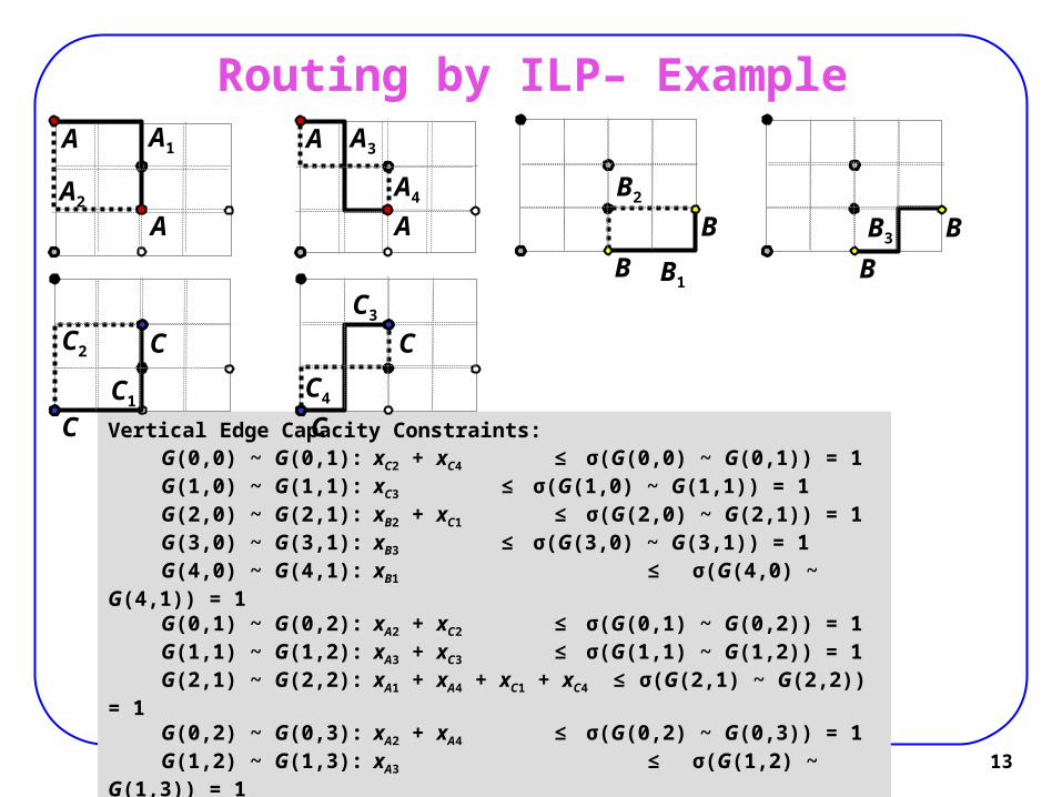
Routing by ILP– Example
Vertical Edge Capacity Constraints:G(0,0) ~ G(0,1): xC2 + xC4 ≤ σ(G(0,0) ~ G(0,1)) = 1G(1,0) ~ G(1,1): xC3 ≤ σ(G(1,0) ~ G(1,1)) = 1G(2,0) ~ G(2,1): xB2 + xC1 ≤ σ(G(2,0) ~ G(2,1)) = 1G(3,0) ~ G(3,1): xB3 ≤ σ(G(3,0) ~ G(3,1)) = 1G(4,0) ~ G(4,1): xB1 ≤ σ(G(4,0) ~ G(4,1)) = 1G(0,1) ~ G(0,2): xA2 + xC2 ≤ σ(G(0,1) ~ G(0,2)) = 1G(1,1) ~ G(1,2): xA3 + xC3 ≤ σ(G(1,1) ~ G(1,2)) = 1G(2,1) ~ G(2,2): xA1 + xA4 + xC1 + xC4 ≤ σ(G(2,1) ~ G(2,2)) = 1G(0,2) ~ G(0,3): xA2 + xA4 ≤ σ(G(0,2) ~ G(0,3)) = 1G(1,2) ~ G(1,3): xA3 ≤ σ(G(1,2) ~ G(1,3)) = 1G(2,2) ~ G(2,3): xA1 ≤ σ(G(2,2) ~ G(2,3)) = 1
A
AA2
A1 A
A
A4
A3
B
B B1
B2
B3 B
B
C
C
C
CC2
C1
C3
C4
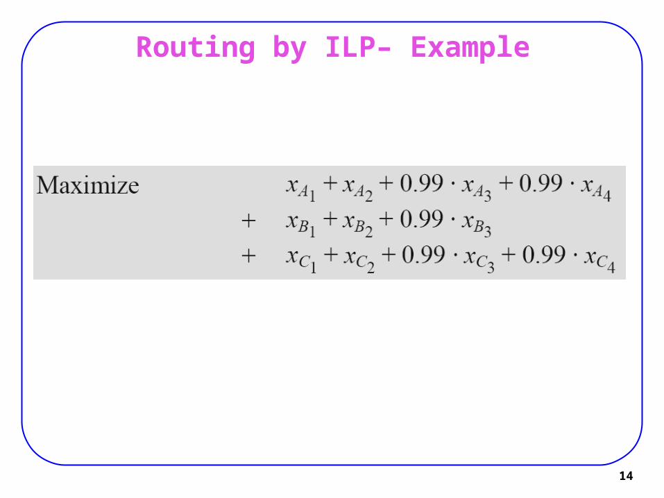
Routing by ILP– Example
14
Routing by ILP
• Complementary techniques:Use two L-shape paths firstThen use maze routing if those paths are not
enough− Sidewinder (2008): runs ILP several times− BoxRouter (2007): maze as postprocess
15
16
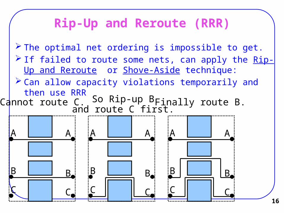
Rip-Up and Reroute (RRR)
The optimal net ordering is impossible to get. If failed to route some nets, can apply the Rip-Up and Reroute or
Shove-Aside technique: Can allow capacity violations temporarily and then use RRR
A
B
C
A
B
C
Cannot route C.
A
B
C
A
B
C
So Rip-up Band route C first.
A
B
C
A
B
C
Finally route B.
18
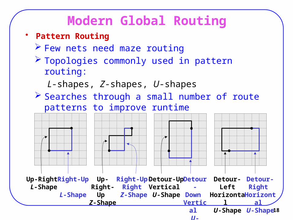
• Pattern Routing Few nets need maze routing Topologies commonly used in pattern routing:
L-shapes, Z-shapes, U-shapes Searches through a small number of route patterns to
improve runtime
Detour-Left
Horizontal U-Shape
Detour-Right
Horizontal U-Shape
Detour-UpVertical U-Shape
Detour-Down
Vertical U-Shape
Up-Right-Up
Z-Shape
Right-Up-Right
Z-Shape
Up-Right L-Shape
Right-Up L-Shape
Modern Global Routing
19
Modern Global Routing
• Negotiation-based router: Each net negotiates the use of shared resources with other
nets until none of the resources are shared• At each iteration:
All nets are routed each using the minimum cost even though leading to over-congestion.
− Costs: according to edge congestion Re-adjust each edge cost based on whether the
corresponding channel has overflowed in the current iteration (and previous iterations).
Route all nets based on this new cost Repeat until all congestion is removed (or some pre-defined
stopping criteria is met:− e.g., maximum number of iterations
20
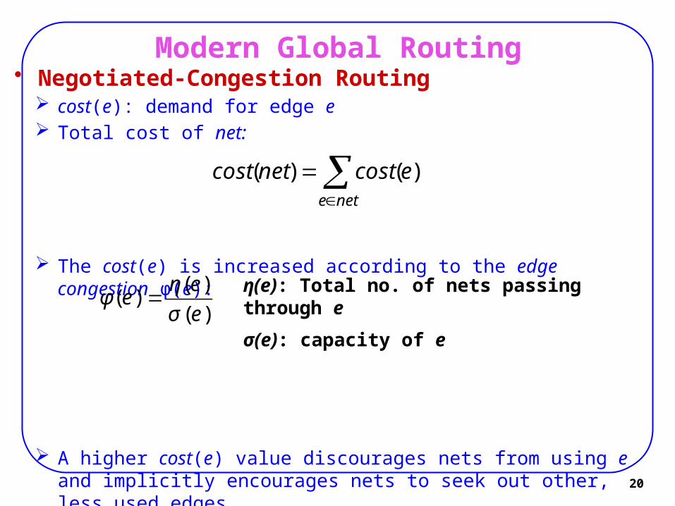
• Negotiated-Congestion Routing cost(e): demand for edge e Total cost of net:
The cost(e) is increased according to the edge congestion φ(e):
A higher cost(e) value discourages nets from using e and implicitly encourages nets to seek out other, less used edges
Þ Iterative routing approaches (Dijkstra’s, A* search, etc.) find routes with minimum cost while respecting edge capacities
nete
ecostnetcost )()(
)(
)()(
eσ
eηeφ
Modern Global Routing
η(e): Total no. of nets passing through e
σ(e): capacity of e
21
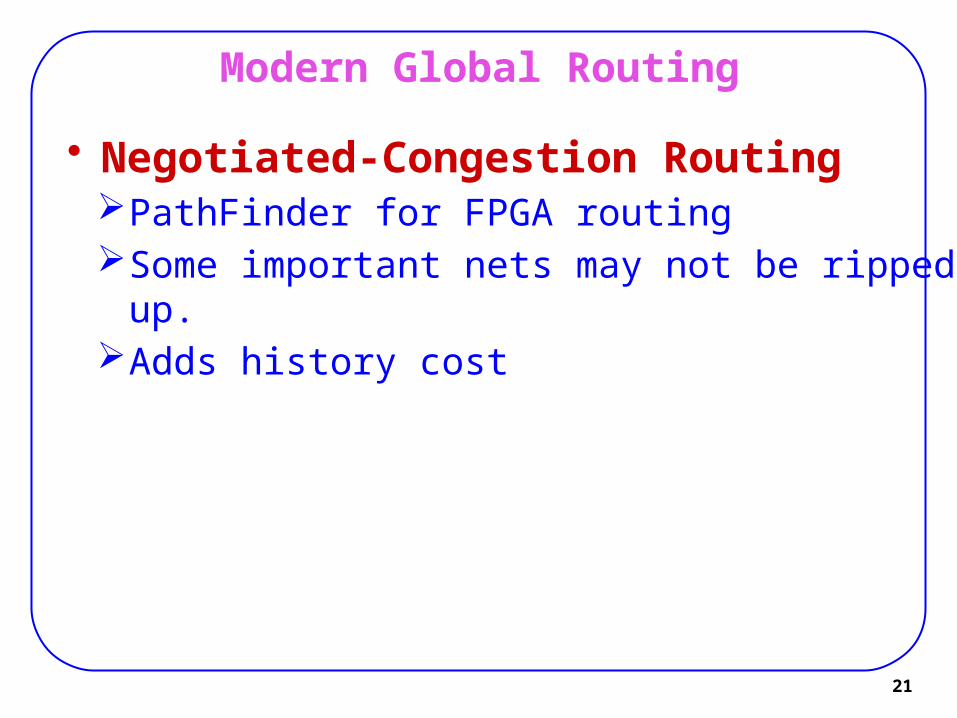
• Negotiated-Congestion RoutingPathFinder for FPGA routingSome important nets may not be ripped up.Adds history cost
Modern Global Routing
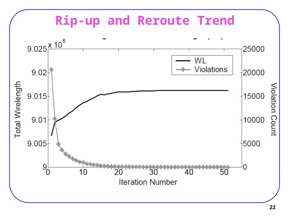
Rip-up and Reroute Trend
22
23
Summary: Types of Routing
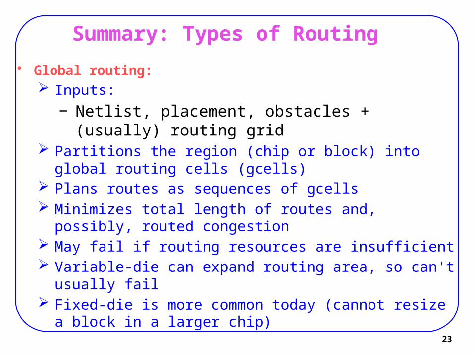
• Global routing: Inputs:
− Netlist, placement, obstacles + (usually) routing grid Partitions the region (chip or block) into global routing cells
(gcells) Plans routes as sequences of gcells Minimizes total length of routes and, possibly, routed
congestion May fail if routing resources are insufficient Variable-die can expand routing area, so can't usually fail Fixed-die is more common today (cannot resize a block in a
larger chip)

24
Summary: Types of Routing
• Interpreting failures in global routing Failure with many violations => must restructure the netlist
and/or redo global placement Failure with few violations => detailed routing may be able to fix
the problems
25
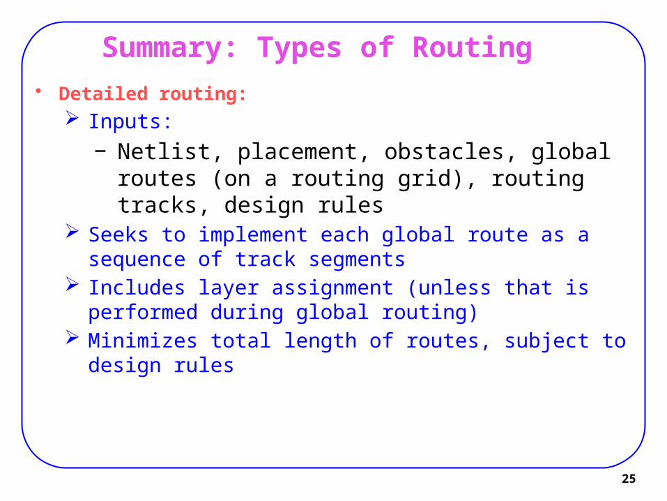
Summary: Types of Routing • Detailed routing:
Inputs:
− Netlist, placement, obstacles, global routes (on a routing grid), routing tracks, design rules
Seeks to implement each global route as a sequence of track segments
Includes layer assignment (unless that is performed during global routing)
Minimizes total length of routes, subject to design rules
26
Summary: Types of Routing
• Timing-driven routing: Minimizes circuit delay by optimizing timing-critical nets Usually needs to trade off route length and congestion
against timing Both global and detailed routing can be timing-driven
27
Summary: Types of Routing
• Large net routing:Nets with many pins can be so complex that
routing a single net warrants dedicated algorithmsSteiner tree construction:
− Minimum wirelength, extensions for obstacle-avoidance
Large signal nets are split into smaller segments processed during detailed routing
• Clock Tree Routing / Power Routing:Performed before global routing to avoid
competition for resources occupied by signal nets
28
Summary: Routing Single Nets
• Single net routing: Usually ~50% of the nets are two-pin nets, ~25% have three
pins, ~12.5% have four, etc. Two-pin nets can be routed as L-shapes or using maze search Three-pin nets usually have 0 or 1 branching point Larger nets are more difficult to handle
29
Summary: Routing Single Nets
• Pattern routing For each net, considers only a small number of shapes (L, Z,
U, T, E) Very fast, but misses many opportunities Good for initial routing, sometimes is sufficient
• Routing pin-to-pin connections Breadth-first-search (when costs are uniform) Dijkstra's algorithm (non-uniform costs) A*-search (non-uniform costs and/or using additional distance
information)

30
Summary: Routing Single Nets
• MST and SMT in the rectilinear topology RMSTs can be constructed in near-linear time Constructing RSMTs is NP-hard, but feasible in
practice For nets with <10 pins, RSMTs can be found using
look-up tables (FLUTE) very quickly

31
Summary: Full Netlist Routing
• Routing by ILP Capture the route of each net by 0-1 variables, form equations
constraining those variables The objective function can represent total route length Solve the equations while minimizing the objective
function (ILP software) Usually a convenient but slow
− May not scale to largest netlists − Can be extended by area partitioning
32
Summary: Full Netlist Routing
• Rip-up and Re-route (RRR) Processes one net at a time, usually by A*-search and
Steiner-tree heuristics Allows temporary overlaps between nets When every net is routed (with overlaps), it removes (rips up)
those with overlaps and routes them again with penalty for overlaps
This process may not finish, but often does, else use a time-out
33
Summary: Full Netlist Routing
• ILP and RRR: Both can be applied in global and detailed routing ILP-based routing is usually preferable for small, difficult-to-
route regions RRR is much faster when routing is easy
34
Summary: Modern Global Routing
• Modern global routing: Initial routes are constructed quickly by pattern routing and
the FLUTE package for Steiner tree construction - very fast Several iterations based on modified pattern routing to avoid
congestion - also very fast
− Sometimes completes all routes without violations− If violations remain, they are limited to a few
congested spots
35
Summary: Modern Global Routing
• Modern global routing: The main part of the router is based on a variant of RRR
called Negotiated-Congestion Routing (NCR)
− Several proposed alternatives are not competitive NCR maintains "history" in terms of which regions attracted
too many nets NCR increases routing cost according to the historical
popularity of the regions
− The nets with alternative routes are forced to take those routes
− The nets that do not have good alternatives remain unchanged
Speed of increase controls tradeoff between runtime and route quality