global solutions of functional fixed point equations via

Global solutions of functional fixed pointequations via pseudo-spectral methods

Benjamin Knorrin collaboration with Julia Borchardt

Theoretisch-Physikalisches InstitutFriedrich-Schiller-Universitat Jena

Asymptotic Safety Seminar04/13/15

work based on arXiv:1502.07511

Research Training GroupQuantum and Gravitational Fields

http://arxiv.org/abs/1502.07511

http://www.uni-jena.de/en/start.html

http://www.qgf.uni-jena.de/

2/17

Outline Motivation Basics of pseudo-spectral methods Examples Summary

Outline

MotivationBasics of pseudo-spectral methodsO(1) model in d=3 and d=2.4Gross-Neveu model in d=3Scalar-tensor model in d=3 (see also last talk by G. P. Vacca)Quo vadis f(R)-gravity?Summary and Outlook

B. Knorr TPI Uni JenaGlobal solutions of functional fixed point equations via pseudo-spectral methods

3/17


Motivation

generic situation in FRG-business: non-linear coupledODEs/PDEs that capture critical physics near fixed pointstandard treatment: local expansions or shooting methoddownside: expensive, global aspects hard to calculateidea: expand in orthogonal polynomials that are defined onwhole interval⇒ (rational) Chebyshev polynomials


4/17


Basics of pseudo-spectral methods I

for simplicity, stick to R+

reminder: Chebyshev polynomials (of first kind):

Tn(cos(x)) := cos(nx)

rational Chebyshev polynomials:

Rn(x) := Tn

(x − Lx + L

), L > 0

divide R+ into two regions:x ∈ [0, x0]: Chebyshev polynomialsx ∈ [x0,∞]: rational Chebyshev polynomials


5/17


Basics of pseudo-spectral methods II

thus, expand any function f via

f (x) =

Nc∑i=0

ciTi(2xx0− 1), x ≤ x0 ,

f∞(x)Nr∑i=0

riRi(x − x0), x ≥ x0 ,

two free numerical parameters:x0: matching point, should be large enough that essentialphysics “happens” for x < x0L: encodes the specific compactification

both parameters can be used to optimize numericalconvergence


6/17


Basics of pseudo-spectral methods III

evaluation of a Chebyshev series via recursive Clenshawalgorithmcalculation of derivative of a Chebyshev series via recursivealgorithm (again yields Chebyshev series)coefficients of the series encode the convergence propertiesand deliver estimate on (series) truncation errorfor “sufficiently nice” functions: exponential convergence,i.e. series coefficients decrease exponentially fast


7/17


Taylor expansion vs. Chebyshev expansion

-1.0 -0.5 0.0 0.5 1.0

-0.4

-0.2

0.0

0.2

0.4

Re z

Im z Domain of convergenceChebyshev expansionTaylor expansion


8/17


Questions?


9/17


O(1) model in d=3, LPA and LPA’

LPA

LPA'

0 1100

140

120

110

16

14

13

12

1 ∞

-16

0

15

12

1

2

4

10∞

ρ

u'*(ρ)


10/17


O(1) model in d=3, eigenperturbations in LPA’

θ=1.548

θ=-0.6127

θ=-3.073

θ=-5.738

θ=-8.551

0.00 0.02 0.04 0.06 0.08

-4

-2

0

2

4

ρ

δu'(ρ)

0 1

10

1

3

1

2

2

31 2 4 10 ∞

-∞

-1000

-500

-250

0

250

500

1000

∞


11/17


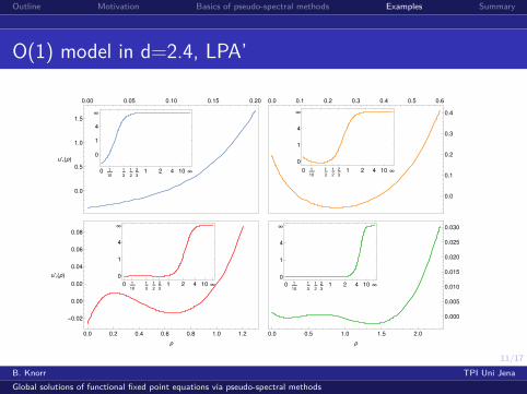
O(1) model in d=2.4, LPA’

0.0

0.5

1.0

1.5

0.00 0.05 0.10 0.15 0.20

u'*(ρ)

0 110

13

12

23

1 2 4 10 ∞

0

1

4

∞

0.0 0.1 0.2 0.3 0.4 0.5 0.6

0.0

0.1

0.2

0.3

0.4

0 110

13

12

23

1 2 4 10 ∞

0

1

4

∞

0.0 0.2 0.4 0.6 0.8 1.0 1.2

-0.02

0.00

0.02

0.04

0.06

0.08

ρ

u'*(ρ)0 1

1013

12

23

1 2 4 10 ∞

0

1

4

∞

0.0 0.5 1.0 1.5 2.0

0.000

0.005

0.010

0.015

0.020

0.025

0.030

ρ

0 110

13

12

23

1 2 4 10 ∞0

1

4

∞


12/17


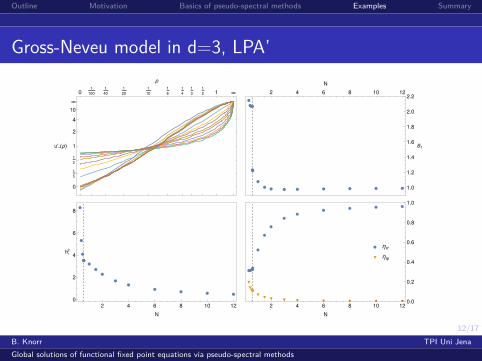
Gross-Neveu model in d=3, LPA’

0

15

12

1

2

4

10

∞

01

100140

120

110

16

14

13

12 1 ∞

u'*(ρ)

ρ

2 4 6 8 10 12

1.0

1.2

1.4

1.6

1.8

2.0

2.2

N

θ1

2 4 6 8 10 120

2

4

6

8

N

h*2

●●●●●●

●

●

●

●●

● ● ● ●

▼▼▼▼▼▼

▼ ▼ ▼ ▼ ▼ ▼ ▼ ▼ ▼

● ησ

▼ ηψ

2 4 6 8 10 120.0

0.2

0.4

0.6

0.8

1.0

N


13/17


Scalar-tensor model in d=3

0.00 0.05 0.10 0.15 0.20

0.01

0.02

0.03

0.04

0.05

ρ

v*(ρ)0 1

1014

12

1 2 4 10∞

14

124∞

0.00 0.05 0.10 0.15 0.20

0.07

0.08

0.09

0.10

0.11

0.12

0.13

ρ

f*(ρ)0 1

1014

12

1 2 4 10∞

14

124∞


14/17


Scalar-tensor model in d=3, eigenperturbations

0.00 0.02 0.04 0.06 0.08 0.10

-5

0

5

10

ρ

δv(ρ)

0.00 0.02 0.04 0.06 0.08 0.10

-20

0

20

40

60

ρ

δf(ρ)

θ1 = 3 , θ2 = 1.913 , θ3 = 1.180 ,θ4 = 0.6679 , θ5 = −0.2812 , θ6 = −1.217


15/17


The problem with f(R)-gravity

choice of regulator impedes globally well-defined solution(s)problem lies in “spectral adjusting”in case of f(R):

RTT ∝ f ′(R)

local solutions give some evidence that for some R0,f ′(R0) = 0→ regulator changes sign, proper regularization questionablesimilar in scalar-tensor model


16/17


Summary

pseudo-spectral methods are handy to represent solutions tofixed point equations

globally,with high precision,efficiently

perturbations to fixed point equations can be resolved in thatway as well → high-precision critical exponentsapplication to flows: stay tuned


17/17


Controversial statement(s)

local expansions are uncontrolled (anyway, we want to donon-perturbative physics!)shooting method gets expensive very fast (starting values forevery operator, anomalous dimensions self-consistenly, . . . )(global) spectral methods solve both problems

Thank you for your attention!


global solutions of functional fixed point equations via

Documents