Global Stokes Drift andClimate Wave Modeling

Adrean Webb

University of Colorado, BoulderDepartment of Applied Mathematics

February 20, 2012

In Collaboration with: Baylor Fox-Kemper, Natasha Flyer

Research funded by: NASA ROSES Physical Oceanography NNX09AF38G

1 / 15

Conclusions

Hierarchy of Stokes Drift Approximations:1. 2D spectral data known: Use first-order 2D Stokes drift

???y Random Error ⇠ 10%

2. 1D spectral data known: Use 1D wave spread approximation

I 1D Unidirectional approximation is not advised since it systematicallyoverestimates the 2D Stokes drift by approximately 33%

3. Third-spectral-moment known: Same as 1D wave spread at the surface???y Random Error ⇠ 10%

4. Third-spectral-moment unknown: Use the second moment to empiricallyapproximate the third moment

Climate Wave Model:1. Unstructured node approach removes advective and directional singularities

2. Prototype model shows promise in great circle test case

2 / 15

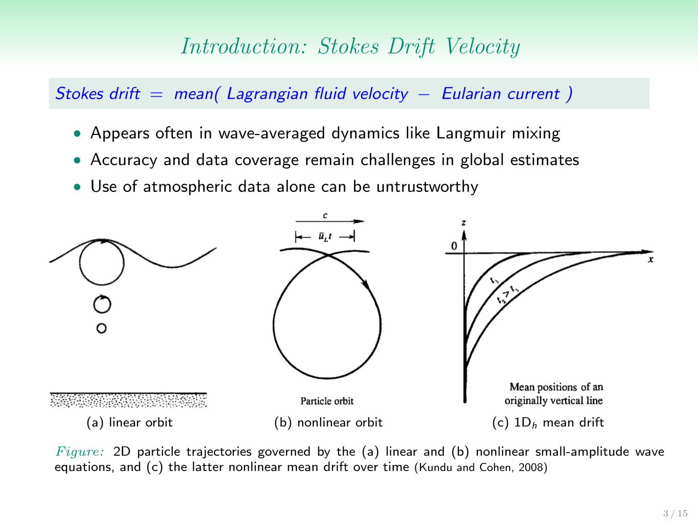
Introduction: Stokes Drift Velocity

Stokes drift = mean( Lagrangian fluid velocity � Eularian current )

• Appears often in wave-averaged dynamics like Langmuir mixing

• Accuracy and data coverage remain challenges in global estimates

• Use of atmospheric data alone can be untrustworthy

(a) linear orbit (b) nonlinear orbit (c) 1Dh mean drift

Figure: 2D particle trajectories governed by the (a) linear and (b) nonlinear small-amplitude waveequations, and (c) the latter nonlinear mean drift over time (Kundu and Cohen, 2008)

3 / 15

Motivation: Importance for Climate Research

There is a persistent, shallow mixed layer bias in the Southern Ocean in globalclimate models (GCM): Langmuir mixing missing???

• Stokes drift plays a dominant role indetermining the strength of Langmuirmixing

I 1/La2t ⇠ us(z = 0)/u⇤

• Langmuir mixing is not currently inany GCM [2/2012]

Figure: Mixed layer depth bias is re-duced in CCSM 3.5 model runs

4 / 15

Lower First-order Stokes Drift Approximations

Overview:

• Survey and error analysis of lower first-order Stokes driftapproximations (spectral moments)

• Comparison of surface Stokes drift estimates using di↵erent dataproducts (e.g., satellites, buoys, models) = Factor of 50% di↵erence!

5 / 15

2011

Global Wave Variable Examples

6 / 15

Stokes Drift and Wave Spectra Examples

The first-order Stokes drift magnitude depends both on the directionalcomponents of the wave field and the directional spread of wave energy

u

S ⇡ 16⇡3

g

Z 1

0

Z ⇡

�⇡

⇣cos ✓, sin ✓, 0

⌘f 3Sf ✓(f , ✓) e

8⇡2 f 2

g z d✓df (1)

16.4. OCEAN-WAVE SPECTRA 285

0

10

30

50

60

80

90

110

100

70

40

20

0 0.05 0.10 0.15 0.20 0.25 0.30 0.35Frequency (Hz)

Wave

Spect

ral D

ensi

ty (

m2

/ H

z)

20.6 m/s

18 m/s

15.4 m/s

12.9 m/s

10.3 m/s

Figure 16.7 Wave spectra of a fully developed sea for di�erentwind speeds according to Moskowitz (1964).

Pierson-Moskowitz Spectrum Various idealized spectra are used to answerthe question in oceanography and ocean engineering. Perhaps the simplest isthat proposed by Pierson and Moskowitz (1964). They assumed that if thewind blew steadily for a long time over a large area, the waves would come intoequilibrium with the wind. This is the concept of a fully developed sea. Here, a“long time” is roughly ten-thousand wave periods, and a “large area” is roughlyfive-thousand wave lengths on a side.

To obtain a spectrum of a fully developed sea, they used measurements ofwaves made by accelerometers on British weather ships in the north Atlantic.First, they selected wave data for times when the wind had blown steadily forlong times over large areas of the north Atlantic. Then they calculated the wavespectra for various wind speeds (figure 16.7), and they found that the function

S(�) =�g2

�5exp

���

��0

�

�4�

(16.28)

was a good fit to the observed spectra, where � = 2�f , f is the wave frequencyin Hertz, � = 8.1 � 10�3, � = 0.74 , �0 = g/U19.5 and U19.5 is the wind speedat a height of 19.5 m above the sea surface, the height of the anemometers onthe weather ships used by Pierson and Moskowitz (1964).

For most airflow over the sea the atmospheric boundary layer has nearly

Figure: Examples of wave spectra: (a) 2D spectra generated by WAVEWATCH III, (b) idealizeddirectional spread (Holthuijsen), and (c) 1D Pierson and Moskowitz observational spectra (Stewart)

7 / 15

Stokes Drift and Multidirectional Waves

Example: Consider a bichromatic spectrum with the same amplitude and peak

frequency for each monochromatic wave but separated by an angle of incidence ✓0.

u

S ⇡ 16⇡3

g

Z 1

0

Z ⇡

�⇡

⇣cos ✓, sin ✓, 0

⌘f 3Sf ✓(f , ✓) e

8⇡2 f 2

g z d✓df

Then the following relation holds1:

u

Sbi 6= 2 u

Smono

= 2�cos ✓0, 0, 0

�u

Smono

1The mean wave direction is along the x-axis

Figure: Example of how the directional com-ponents of a wave field a↵ect the magnitude ofStokes drift

8 / 15

2θ’

Stokes Drift: Improving 1D Estimates

Stokes drift error due to wave spreading in 1D approximates can be minimizedby first recreating the 2D wave spectrum

Idea: Use an empirical directional distribution (Df ) to recover the 2D spectrum

Z 1

0

Z ⇡

�⇡

Sf ✓(f , ✓) d✓df =

Z 1

0

Z ⇡

�⇡

Df (f , ✓) d✓

�Sf (f ) df =

Z 1

0

Sf (f ) df

�! �

16.4. OCEAN-WAVE SPECTRA 285

0

10

30

50

60

80

90

110

100

70

40

20

0 0.05 0.10 0.15 0.20 0.25 0.30 0.35Frequency (Hz)

Wa

ve S

pe

ctra

l De

nsi

ty (

m2

/ H

z)

20.6 m/s

18 m/s

15.4 m/s

12.9 m/s

10.3 m/s

Figure 16.7 Wave spectra of a fully developed sea for di�erentwind speeds according to Moskowitz (1964).

Pierson-Moskowitz Spectrum Various idealized spectra are used to answerthe question in oceanography and ocean engineering. Perhaps the simplest isthat proposed by Pierson and Moskowitz (1964). They assumed that if thewind blew steadily for a long time over a large area, the waves would come intoequilibrium with the wind. This is the concept of a fully developed sea. Here, a“long time” is roughly ten-thousand wave periods, and a “large area” is roughlyfive-thousand wave lengths on a side.

To obtain a spectrum of a fully developed sea, they used measurements ofwaves made by accelerometers on British weather ships in the north Atlantic.First, they selected wave data for times when the wind had blown steadily forlong times over large areas of the north Atlantic. Then they calculated the wavespectra for various wind speeds (figure 16.7), and they found that the function

S(�) =�g2

�5exp

���

��0

�

�4�

(16.28)

was a good fit to the observed spectra, where � = 2�f , f is the wave frequencyin Hertz, � = 8.1 � 10�3, � = 0.74 , �0 = g/U19.5 and U19.5 is the wind speedat a height of 19.5 m above the sea surface, the height of the anemometers onthe weather ships used by Pierson and Moskowitz (1964).

For most airflow over the sea the atmospheric boundary layer has nearly

9 / 15

Higher Order: Comparison of 2D and 1D Estimates

(a) Mag: 1D Unidirectional (x) vs 2D (y) (cm/s)

(c) Mag: 1D Unidirectional (x) vs 1D Spread (y) (cm/s)

(b) Mag: 1D Spread (x) vs 2D (y) (cm/s)

(d) Dir: Mean Wave (x) vs Stokes Drift (y) (rad)

10 / 15

m = 0.8

Current State: Third-generation Wave Models

Figure: Spatial and spectralgrid examples

Current Model Basics:

• Uses structured grids (lat-lon, polar)

• Includes extensive physics and parameterizations

Current Model Deficiencies:

• Spatial and spectral singularities near the poles

• Performance declines as N/S boundaries aremoved higher (presently ±75�)

• Designed to forecast weather not climate

Lat-lon grids:

G3: 2.4 ⇥ 3G4: 3.2 ⇥ 4

Figure: WAVEWATCH III grid performance withbenchmarking targets for coupling to NCAR CESM

11 / 15

Unstructured Approach: RBF-Generated Finite Di↵erences

Figure: Possible node layout

Figure: Great circle propagation

RBF-Generated Finite Di↵erence Method (RBF-FD):

• Solves advective problems with near spectralaccuracy

• Uses an unstructured node layout

• Allows geometric flexibility and local noderefinement

• No advective and directional singularities

• Computational costs are spread equally

• Possibly well-suited for parallelization

Great Circle Propagation Test Case:

• 20 spatial x 10 spectral nodes

• Dissipation and dispersion error after 0.5 cycles

I Third-order upwind ⇠ 0.2

I Radial Basis Functions ⇠ 0.5x10�4

12 / 15

Conclusions

Hierarchy of Stokes Drift Approximations:1. 2D spectral data known: Use first-order 2D Stokes drift

???y Random Error ⇠ 10%

2. 1D spectral data known: Use 1D wave spread approximation

I 1D Unidirectional approximation is not advised since it systematicallyoverestimates the 2D Stokes drift by approximately 33%

3. Third-spectral-moment known: Same as 1D wave spread at the surface???y Random Error ⇠ 10%

4. Third-spectral-moment unknown: Use the second moment to empiricallyapproximate the third moment

Climate Wave Model:

1. Unstructured node approach removes advective and directional singularities

2. Prototype model shows promise in great circle test case

13 / 15

Thank You!

14 / 15

References

Stokes Drift:

• Webb, A., Fox-Kemper, B., 2011. Wave Spectral moments and Stokesdrift estimation. Ocean Modelling, Volume 40.

Langmuir Mixing:

• Fox-Kemper, B., Webb, A., Baldwin-Stevens, E., Danabasoglu, G.,Hamlington, B., Large, WG., Peacock, S., in preparation. Global climatemodel sensitivity to estimated Langmuir Mixing.

RBF-Generated Finite Di↵erence Method:

• Flyer, N., Lehto, E., Blaise, S., Wright, G., A. St-Cyr, 2011.RBF-generated finite di↵erences for nonlinear transport on a sphere:shallow water simulations. Preprint.

• Fornberg, B., Lehto, E., 2011. Stabilization of RBF-generated finitedi↵erence methods for convective PDEs. Journal of ComputationalPhysics, Volume 230, Issue 6.

15 / 15