global warming on japanglobal warming is expected to progress in the coming 20 years regardless of...
TRANSCRIPT

Ministry of the Environment, Japan Global Environment Research Fund Strategic R&D Area Project
S‐4 Comprehensive Assessment of Climate Change Impacts to Determine the Dangerous Level of Global Warming and Appropriate Stabilization Target of
Atmospheric GHG Concentration Second Report
Global Warming Impacts on Japan – LongTerm Climate Stabilization Levels and Impact Risk Assessment –
May 2009 Project Team for Comprehensive Projection of
Climate Change Impacts
Ibaraki University, National Institute for Environmental Studies,
Tohoku University, Meijo University,
National Institute for Rural Engineering, The University of Tokyo,
National Institute for Land and Infrastructure Management, University of Tsukuba,
National Institute of Infectious Diseases, National Institute for Agro‐Environmental Sciences,
Japan International Research Center for Agricultural Sciences, Forestry and Forest Products Research Institute,
Kyushu University, The Institute of Statistical Mathematics

Introduction This report is the second report of the Global Environment Research Fund Strategic R&D Area Project entitled “S‐4 Comprehensive Assessment of Climate Change Impacts to Determine the Dangerous Level of Global Warming and Appropriate Stabilization Target of Atmospheric GHG Concentration” (abbreviated title: “Project for Comprehensive Projection of Climate Change Impacts”) being implemented by the Ministry of the Environment, Japan, which is a compilation of the research results up to the fourth year of the project (fiscal 2005‐2008). Initiated in 2005, this research project has a total term of five years comprising a first period of three years followed by a second, two‐year period with the objectives of “carrying out comprehensive research concerning climate change impacts on the Asian region including Japan and obtaining a quantitative overview of these impacts, determining the dangerous level of global warming impacts based on these results, and presenting scientific findings on emission stabilization paths.” This report presents new research results obtained since the first report of this project was released on May 29, 2008, entitled Global Warming Impacts on Japan–Latest Scientific Findings. Compared with the 2008 research report, the present report is characterized by the following three features: (1) Impact assessments by stabilization level of atmospheric GHG concentration, performed using
an integrated assessment model. (2) Assessments of regional‐level in addition to nationwide impacts. (3) Assessments of damage costs in addition to physical impacts. The research results presented here are scientific findings concerning the dangerous level of global warming of which there are few comparable examples in the world. With the forthcoming COP15 in December this year, many studies and negotiations on the international framework from 2013 onward are taking place worldwide including in Japan. At such a time, it is our hope that the present research results will be widely applied in determining which temperature rise level is considered to be “a level that would prevent dangerous anthropogenic interference with the global climate system,” as well as in studying adaptation measures for unavoidable adverse effects, and other related issues. On behalf of the Project Team for Comprehensive Projection of Climate Change Impacts Nobuo MIMURA S‐4 Research Project Leader (Institute for Global Change Adaptation Science (ICAS), Ibaraki University) May 29, 2009

Contents
3
Contents
Introduction Contents・・・・・・・・・・・・・・・・・・・・・・・・・・・・・・・・・ 3
Main Research Results・・・・・・・・・・・・・・・・・・・・・・ 4
Objectives and Outline of Report・・・・・・・・・・・・・・ 5
I. Outline of Integrated Assessment
1.1 Outline of Integrated Assessment Model・・・・ 7
(1) AIM/Impact[Policy] integrated assessment model ・・・ 7 (2) Impact assessment and adaptation model・・・・・・ 7 (3)Impact assessment procedure・・・・・・・・・・・ 8
1.2 Outline of Stabilization Scenarios・・・・・・・・ 9
1.3 Targeted Regions/Periods・・・・・・・・・・・・・・ 10
1.4 Points to be Noted・・・・・・・・・・・・・・・・・・・ 10
II. Climate Change Impacts by Field
1. Impacts of Floods ・・・・・・・・・・・・・・・・・・・ 11
1.1 Estimation Method ・・・・・・・・・・・・・・・・・・・ 11
1.2 Future Impacts・・・・・・・・・・・・・・・・・・・・・・・・ 12
(1) Flooded area・・・・・・・・・・・・・・・・・・・・・・ 12 (2) Flood damage cost potential ・・・・・・・・ 13
2. Impacts of Landslide Disasters・・・・・・・・・ 14
2.1 Estimation Method・・・・・・・・・・・・・・・・・・・・・ 14
2.2 Future Impacts・・・・・・・・・・・・・・・・・・・・・・・・ 15
(1) Probability of slope failure・・・・・・・・・・・・・・・ 15 (2) Slope failure damage cost potential・・・・ 16
3. Suitable Habitats for F. crenata Forests・・・ 17
3.1 Estimation Method・・・・・・・・・・・・・・・・・・・ 17
3.2 Future Impacts ・・・・・・・・・・・・・・・・・・・・・ 18
(1) Suitable habitats for F. crenata forests・・・・・・・ 18 (2) Cost of damage due to decrease in suitable
habitats for F. crenata forests・・・・・・・ 19
4. Areas at Risk of Pine Wilt・・・・・・・・・・・・・・ 20
4.1 Estimation Method・・・・・・・・・・・・・・・・・・・・・・・・・・・・ 20
4.2 Future Impacts・・・・・・・・・・・・・・・・・・・・・・・・・・・・ 21 (1) Areas at risk of pine wilt・・・・・・・・・・・・・・・・・ 21
5. Rice Yield・・・・・・・・・・・・・・・・・・・・・・・・・・・ 22
5.1 Estimation Method・・・・・・・・・・・・・・・・・・・・・ 22
5.2 Future Impacts・・・・・・・・・・・・・・・・・・・・・・・・ 23 (1) Rice yield・・・・・・・・・・・・・・・・・・・・・・・・・ 23 (2) Rice yield variation・・・・・・・・・・・・・・・・・ 24
6. Sand Beach Loss due to Sea Level Rise・・・・ 25 6.1 Estimation Method・・・・・・・・・・・・・・・・・・・・・ 25 6.2 Future Impacts・・・・・・・・・・・・・・・・・・・・・・・・ 26 (1) Cost of damage due to sand beach loss・・・・・・・・・ 26
7. Damage due to storm‐surge flooding・・・・・ 27 7.1 Estimation Method・・・・・・・・・・・・・・・・・・・・・ 27 7.2 Future Impacts・・・・・・・・・・・・・・・・・・・・・・・・ 28 (1) Affected population, area, and cost of damage due to
storm‐surge flooding・・・・・・・ 28
8. Heat Stress Mortality Risk・・・・・・・・・・・・・・ 30
8.1 Estimation Method・・・・・・・・・・・・・・・・・・・・・ 30
8.2 Future Impacts・・・・・・・・・・・・・・・・・・・・・・・・ 31
(1) Heat stress mortality risk・・・・・・・・・・・・ 31 (2) Cost of damage due to heat stress
(heatstroke) mortality ・・・・・ 32
Reference Materials・・・・・・・・・・・・・・・・・・・・・・・ 33
Members and Contacts ・・・・・・・・・・・・・・・・・・ 38

Main Research Results
4
Main Research Results Main Research Results 1. In Japan as well, even greater impacts of global warming are expected in the future in
a broad range of fields related to people’s lives. If a significant cut in global greenhouse gas (GHG) emissions is achieved, the damage to Japan is also expected to be reduced to a considerable extent. However, even when the GHG concentration is stabilized at 450 ppm, the occurrence of a certain amount of damage is unavoidable.
Climate change impacts have been quantitatively assessed in terms of eight indexes: (1) flooded area and cost of damage due to floods; (2) probability of slope failure and cost of damage due to landslide disasters; (3) impacts on suitable habitats for Fagus crenata (Japanese beech) forests and cost of damage; (4) expansion of areas at risk of pine wilt; (5) impacts on rice yield; (6) expansion of area of sand beach loss and cost of damage; (7) expansion of area of storm‐surge flooding, affected populations, and cost of damage; and (8) heat stress mortality risk and cost of damage. In all indexes, the lower the level at which GHG concentration is stabilized, the lower the adverse impacts will be. Even under the scenario with the strictest stabilization level (GHG concentration 450 ppm), however, it is found that adverse impacts may still occur if appropriate measures are not taken.
Table i Climate scenarios and impacts by stabilization level (nationwide values)
Unit 450s 550s BaU 450s 550s BaU 450s 550s BaUChange in annual temperature (1990=0℃) ℃ 0.9 0.9 1.0 1.3 1.6 1.7 1.6 2.3 3.2
Change in annual mean precipitation (1990=100%) % 100 101 101 105 106 107 107 110 113
Sea level rise (1990=0m) m 0.06 0.07 0.07 0.10 0.11 0.12 0.15 0.19 0.24
Flooded area 1000km2 0.2 0.2 0.2 0.6 0.7 0.7 0.5 0.6 0.8
Food damage cost potential Trillion yen/year 1.3 1.3 1.3 4.4 4.7 4.9 5.1 6.1 8.3
Probability of slope failure % 3 3 3 3 4 4 4 5 6
Slope failure damage cost potential Trillion yen/year 0.60 0.60 0.60 0.49 0.52 0.58 0.65 0.77 0.94
Suitable habitats for F. crenata forests % 79 77 77 72 65 61 64 50 32
Cost of damage due to loss of suitable habitats for F. crenata forests 100 million yen/year 778 829 851 1034 1273 1381 1325 1811 2324
Pine wilt Areas at risk of pine wilt % 15 16 16 22 26 28 27 37 51
Rice Rice yield t/ha 4.9 5.0 5.0 4.9 5.0 5.1 4.8 4.9 5.1
Area of sand beach loss % 13 13 13 19 21 23 29 37 47
Cost of damage due to loss of sand beaches 100 million yen/year 116 118 121 176 192 208 273 338 430
Population affected by storm‐surge flooding (western Japan) 10,000 people/year 12 12 12 19 20 21 32 37 44
Population affected by storm‐surge flooding (Japan's three major bays) 10,000 people/event 11 11 11 17 17 17 30 32 35
Area of storm‐surge flooding (western Japan) km2/year 60 60 61 92 97 102 155 176 207
Area of storm‐surge flooding (Japan's three major bays) km2/event 24 24 24 37 38 39 63 67 72
Cost of damage due to storm‐surge flooding (western Japan) Trillion yen/year 2.0 2.0 2.0 3.1 3.3 3.5 5.4 6.2 7.4
Cost of damage due to storm‐surge flooding (Japan's three major bays) Trillion yen/event 0.2 0.2 0.2 0.3 0.4 0.4 1.8 2.0 2.3
Heat stress mortality risk - 1.5 1.6 1.6 1.8 2.1 2.2 2.1 2.8 3.7
Cost of damage due to heat stress (heatstroke) mortality 100 million yen/year 243 265 274 373 480 529 501 775 1192
Sand beaches
Storm surges
Heat stress
2090s
Landslidedisasters
Fagus crenata(Japanese beech)
Climate scenario/impact field
Floods
2030s 2050s
2. Global warming is expected to progress in the coming 20 years regardless of whether
additional mitigation measures are implemented. However, differences in impacts reflecting differences in the global climate stabilization level are expected to become larger from around mid‐century onward. Therefore, in addition to the active implementation of mitigation measures for stabilizing the climate, it is necessary to study and implement adaptation measures from the long‐term viewpoint without delay in preparation for the occurrence of certain levels of adverse impacts.
The Fourth Assessment Report (AR4) of the Intergovernmental Panel on Climate Change (IPCC) states as follows: “For the next two decades, a warming of about 0.2°C per decade is projected for a range of SRES emission scenarios.” As global warming progresses, its adverse impacts will extend over a prolonged period and a long time will be required for the effects of climate stabilization to appear. Therefore, in order to minimize future damage and avoid passing the burden of measures on to future generations, it is necessary to study and implement adaptation measures from the long‐term viewpoint.

Objectives of Report and Outline of Report
5
Objectives of Report The present report is the second report
presenting the results of the Project for Comprehensive Projection of Climate Change Impacts (Global Environment Research Fund Strategic R&D Area Project entitled “S‐4 Comprehensive Assessment of Climate Change Impacts to Determine the Dangerous Level of Global Warming and Appropriate Stabilization Target of Atmospheric GHG Concentration” being implemented by the Ministry of the Environment, Japan), which was initiated in fiscal 2005.
Targeting the Asian region including Japan, the objectives of this research project are to obtain a quantitative overview of the impacts of climate change, to determine the dangerous level of global warming impacts based on this quantitative overview, and moreover, to estimate the impacts that will appear with various emission stabilization paths.
In the first period of the study during the three years from 2005 to 2007, the methods of impact projection and economic assessment in key fields such as water resources, forests, agriculture, coastal zones, and human health in the Asian region including Japan were developed, focusing on the period from around mid‐century (around 2050) up to the end of the century, and progress was made in the development of an integrated assessment model for comprehensively analyzing impacts and risks. The first interim report, entitled Global Warming Impacts on Japan–Latest Scientific Findings, was released in May 2008. It presented the research results of the first three‐year period, including the regional distributions of impacts occurring in Japan, quantitative data on rates of appearance, etc.
The present report is a compilation of new research results obtained since the first interim report, and is characterized by in the following three points: (1) Impacts on Japan according to the stabilization
level of atmospheric GHG concentration have been assessed using an integrated assessment model.
(2) Impacts have been assessed at the regional level in addition to the nationwide level.
(3) Damage costs have been assessed in addition to physical impacts.
The present report provides a comprehensive overview of how the impacts on Japan and costs of damage differ according to the climate stabilization level. It is our hope that the findings provided in this report will serve as a useful basis for policy decisions and ongoing research in view of the widespread discussions now taking place on the framework of measures against global warming to be implemented from 2013 onward.
Outline of Report This report describes increases in the
impacts of global warming by field under the Business as Usual (BaU) scenario and two scenarios in which GHG concentrations are stabilized at 450 ppm and 550 ppm in terms of carbon dioxide (CO2) equivalent concentration (stabilization scenarios). These two stabilization scenarios correspond to mean temperature rises of roughly 2.1°C (2.1°C in 2100) and 2.9°C (2.7°C in 2100), respectively, compared with prior to the industrial revolution, while the BaU case corresponds to a mean temperature rise of 3.8°C in 2100. Only the value in 2100 is given for BaU, as the equilibrium state of temperature stabilization is not assumed.
The climate change impact functions by field used for these projections were constructed by the research group dealing with each field using impact assessment models developed based on their respective areas of expertise. These climate change impact functions were incorporated into the AIM/Impact[Policy] integrated assessment model in order to make integrated assessments of GHG emission paths, GHG concentrations, temperature rises, and impacts by field, and the impacts in all fields were projected under the three scenarios. The projections include assessments of not only physical and biological impacts but also the costs of damage calculated by converting the impacts into monetary values. Such comprehensive assessments are the result of joint research carried out in close cooperation by the participating researchers.
This report consists of two parts. Part I outlines the integrated assessment model and the stabilization scenarios used in this study. In Part II, the results of quantitative assessments targeted at Japan using the integrated assessment model are presented for the following eight fields: (1) flooded area and cost of damage due to floods; (2) probability of slope failure and slope failure damage cost potential due to landslide disasters; (3) impacts on suitable habitats for F. crenata forests and cost of damage; (4) expansion of areas at risk of pine wilt; (5) impacts on rice yield; (6) expansion of loss of sand beach area and cost of damage; (7) expansion of area of storm‐surge flooding, affected populations, and cost of damage; and (8) heat stress mortality risk and cost of damage.
The impacts of climate change extend over a broad range, as shown in Table ii. In view of the difficulty of quantitatively assessing all of these impacts, however, this project is focusing on a portion of them for physical and economic assessments. Economic assessments of the costs of damage that have been performed up to now have most likely employed a macroeconomic method (treating a wide area as one region, and assuming comparatively

Main Research Results
6
simple equations for estimation). In contrast, the approach taken in the present project has been to model the physical or biological processes of interest and calculate the physical impacts first, then express the values obtained in terms of monetary values. This has made it possible to perform calculations for any given region. Moreover, although the overall impacts may not be grasped as comprehensively as in the macroeconomic method, the estimation results can be considered to be higher in accuracy.
The first interim report released in 2008 presented not only the regional distribution of impacts occurring in Japan (impact maps), but also changes in the occurrence of these impacts for each level of temperature rise. That is, changes in impacts by field and changes in factors other than temperature were consolidated applying MIROC as the climate scenario and using the integrated assessment model for global warming impact assessments, taking 1990 as the base year for representing temperature rise on the x‐axis (Fig. i). The graphs in the first interim report are reproduced
in Fig. i (with slight modifications) to enable comparisons with the results presented in this report.
Table ii List of indexes targeted for climate change impact assessment
Water resources Ecosystems Agriculture
(food) Disaster
prevention Human health
Water shortages (municipal water)
Forest ecosystems
(F. Crenata and pine)
Agriculture (rice) Floods Heat
Water shortages (agricultural
water)
Forest ecosystems(other than F. Crenata and
pine)
Agriculture (other than
rice)
Landslide disasters
Atmospheric
pollution
Water shortages (industrial water)
Alpine plants Fruit trees Storm‐surge
flooding Infectious diseases
Snow water resources
Natural grasslands Tea Liquefaction
Water quality Bogs Vegetables Sand beaches
Groundwater Oceans Livestock
Coasts Marine products
Fresh water Tidal flats
Fig. i Temperature rise and impacts on floods, slope disasters, suitable habitats for F. crenata, area of pine wilt, storm‐surge
flooding, and heat stress mortality risk
0.95
1.00
1.05
1.10
1.15
1.20
Change in
floo
ded
area
0
1
2
3
4
5
Change in expected
damage from
torrential
rainfall on
ce every 50
years
Flooded areaEconomic loss due to flooding
0.98
1.00
1.02
1.04
1.06
1.08
1.10
Change in ave. value
of
slop
e failure risk
0.99
1.00
1.01
1.02
1.03
1.04
1.05
Change
in expected damage
from
torrentia
l rainfall once
every 50
years
Slope failureEconomic loss due to slope failure
1.0
1.5
2.0
2.5
3.0
Change in
area of
pine
wilt
0
50
100
150
200
Shrinkage rate of
suitable habitats fo
r F.
crenata (%
)
Pine wilt
Suitable habitats for F. crenata
80
100
120
140
0.0 1.0 2.0 3.0 4.0 5.0
Annual mean temperature increase in Japan (1990 = 0℃)
Change in sum
mer
mean preciptitation
(199
0=10
0)
80
100
120
140
Change in winter
mean preciptitation
(199
0=10
0)
Summer mean precipitationWinter mean precipitation
0.9
1.0
1.1
Rice yield
Rice yield
350
450
550
650
750
CO2 con
centratio
n
(ppm
)
13.0
13.5
14.0
14.5
15.0
Insolatio
n (M
J/m
2 )
CO2 concentrationInsolation
1.0
1.5
2.0
2.5
3.0
3.5
Change in
area of
storm‐surge floo
ding
1.0
2.0
3.0
4.0
5.0
6.0
Change in
pop
ulation
affected
by storm‐
surge flo
oding
Area of storm‐surge floodingAffected population
1
2
3
4
5
6
Change in
heat stress
mortality risk Heat stress mortality risk
90
100
110
120
130
140
Extrem
e rainfall with
return period of 50 years
(199
0=10
0)
90
100
110
120
130
140
Daily m
ean precipitation
(199
0=10
0)
Extreme rainfall with return period of 50 yearsDaily mean precipitation
0.0
0.2
0.4
0.0 1.0 2.0 3.0 4.0 5.0Annual mean temperature increase in Japan (1990 = 0)
Sea level rise (m
)
Sea level rise
1990 2030 2050 2100
Global annual mean temperature increase (1990=0℃)
0 1.6 2.4 4.4
1990 2030 2050 2100
Global annual mean temperature increase (1990=0℃)
0 1.6 2.4 4.4

I. Outline of Integrated Assessment
7
I. Outline of Integrated Assessment
1.1 Outline of Integrated Assessment Model (1) AIM / Impact [Policy] integrated assessment model The AIM / Impact [Policy] integrated assessment model has been developed and expanded in the Project for Comprehensive Projection of Climate Change Impacts for the purpose of integrative assessing GHG emission paths, GHG concentrations, temperature rises, and impacts by field until 2100 with 1990 as the base year. Using AIM/Impact[Policy], impacts in a time series can be calculated for climate stabilization levels, emission reduction targets, etc. established as policy targets. This makes it possible to examine whether unacceptable levels of serious climate change impacts can be avoided by achieving a certain climate stabilization target. In this context, climate change impact functions, which indicate how the impacts by field appear, were constructed by the research groups for each field based on their respective areas of expertise (refer to Part II).
AIM / Impact [Policy] can be roughly divided into the GHG emission projection model group, and the impact assessment and adaptation model (Fig. I‐1). Using an energy‐economic model incorporated into the GHG emission projection part, the paths of global GHG emissions under various restrictions (global mean GHG concentration, etc.) are estimated by optimization calculations. Here, optimization means that the total obtained by converting the level of utility (consumption) per person at each point of time in the future to the present value using a discount rate, and weighted by population, is optimized in the targeted period. Moreover, using a simplified climate model implemented in the energy‐economic model, changes in global mean temperature under the various restrictions mentioned above are calculated and serve as the input data for the impact assessment and adaptation model.
Next, in the impact assessment and adaptation model, using a normalized climate change database and impact functions by field described in (2) below, climate change (temperature, precipitation, etc.) by region (i.e., by country when used as a global model; by prefecture when used as a model for Japan) and levels of impacts by field are calculated in a time series (Fig. I‐1). (2) Impact assessment and adaptation model
As mentioned above, the impact assessment and adaptation model of AIM/Impact[Policy] projects climate change and climate change impacts according to each field by region (i.e., by country or by prefecture) in a time series with global mean temperature change as the input condition. The methodology that is mainly used for projecting the future impacts of global warming comprises division of the space concerned into squares at even intervals in the latitudinal and longitudinal directions (thereby forming a mesh); calculation of the required data such as temperature, precipitation, soil moisture, and various other factors for each mesh; and then, using these data as conditions, estimation of the impacts using a model that represents physical, chemical, and ecological processes (hereafter referred to as an “impact factor model”).
This method of impact assessment using a mesh has an advantage in that the spatial distribution of impacts can be shown in detail. On the other hand, the higher the spatial resolution, the larger the calculation loads. To overcome this problem, a technique has been devised for the impact assessment and adaptation model whereby a regional‐level normalized climate change database and impact functions by field are prepared in advance, and then used for the impact assessments.
The normalized climate change database is a representation of future quantitative changes in climatic variables of each region (temperature, precipitation, insolation, etc.) in terms of their ratio to quantitative global mean climate changes. That is, using climate projections by a global climate model (GCM), spatially averaged quantitative changes in climatic variables are determined by country or by prefecture, and the ratios are obtained by dividing these values by the global mean temperature change during the same period. When this is combined with a global mean temperature scenario transferred from the simplified climate model implemented in the energy‐economic model, future climate scenarios by country or by prefecture can be created using the technique of pattern scaling, which is described later.
In this connection, since the spatial resolution of the original GCM numerical simulation results is low, simple spatial interpolation of the GCM numerical simulation results into 2’30” spatial mesh data in the horizontal direction is performed first, then the spatial average by country (or by prefecture) is estimated.
GCM simulation results using a total of 30

I. Outline of Integrated Assessment
8
GCMs and 77 scenarios provided by the Program for Climate Model Diagnosis and Intercomparison (PCMDI) of the IPCC Data Distribution Centre (IPCC‐DDC) have been collected, systematized, and stored in the normalized climate change database up to the present time.
An impact function, whose purpose is to show how a given impact changes in accordance with changes in climatic factors such as temperature, precipitation, etc., in actuality comprises a database of collected paired data (climatic factors and impacts). In the process of its preparation, numerous simulations are performed by varying climatic factors in certain increments, and the outputs estimated by the impact factor model are averaged by region and totaled. The advantage of impact functions is that the climate scenario (time series of climate change) is given by region, allowing the time series of impact changes to be quickly calculated. This makes it easy to examine the levels of impacts for various emission reduction policies. On the other hand, it should also be noted that (1) only climatic factors varied by sensitivity analysis can be taken into consideration, and (2) since totals are obtained by region, spatial differences within a region become equalized. In this research project, each of the groups researching impacts by field is jointly developing impact functions according to their field by country (in the case of global impacts) or by prefecture (in the case of impacts on Japan), and the impact functions
constructed in this way are implemented in the impact assessment and adaptation model (Table I‐1). (3) Impact assessment procedure
Figure I‐1 shows the impact assessment procedure using AIM / Impact [Policy]. When a global mean temperature change scenario is transferred from the energy‐economic model of AIM / Impact [Policy], first a climate scenario by country or by prefecture is created by pattern scaling. Pattern scaling is a method in which the spatial distribution of climatic factors is represented by the results of GCM simulation. Global warming under multiple emission scenarios is calculated using a simple temperature rise estimation model, which does not calculate to the extent of the spatial distribution of climatic factors. Therefore, if the spatial distribution of climatic factors is determined in advance according to global mean temperature changes, the desired values can be easily obtained. In the pattern scaling of AIM/Impact[Policy], the normalized climate change database is used with the temperature change and precipitation change obtained from the GCM simulation results as patterns.
Then, by inputting the climate scenario by country or by prefecture into the impact functions by field prepared for each country/region, the impacts by field according to the country or region are calculated.
Fig. I‐1 Schematic diagram of global multiregional and multisectoral impact assessment and adaptation
model (database type model)
Pattern scaling
Global mean temperaturechange scenario
Climate scenario by country/by prefecture
PCMDI
IPCC‐DDCNormalized climate change database by country/by prefecture
Climate change impact assessment by country/by prefecture (by field)
Targeted area (Japan)
FloodsLandslide disastersSuitable habitats for
F. crenata forestsAreas at risk of pine wiltRice yieldStorm‐surge floodingHeat stress mortality risk
Changes in potential productivity (maize)Changes in potential productivity (wheat)Changes in potential productivity (rice)Water withdrawal to water resources ratio
(population under high water stress)Water withdrawal to water resources ratio
(population under medium water stress)Water withdrawal to water resources ratio
(population under low water stress)Falkenmark index (population under high water stress)Falkenmark index (population under medium water stress)Heat stress mortality risk
Targeted area (world)
•The impact calculation procedure using AIM/Impact[Policy] is shown inside the solid lines.
Map of climate change impacts by country (by field)
Map of climate change impacts by prefecture (by field)
Climate change impact function
*The part incorporated into AIM/Impact[Policy] by prior preparation is shown inside the dotted lines.
Pattern scaling
Global mean temperaturechange scenario
Climate scenario by country/by prefecture
PCMDI
IPCC‐DDCNormalized climate change database by country/by prefecture
Climate change impact assessment by country/by prefecture (by field)
Targeted area (Japan)
FloodsLandslide disastersSuitable habitats for
F. crenata forestsAreas at risk of pine wiltRice yieldStorm‐surge floodingHeat stress mortality risk
Changes in potential productivity (maize)Changes in potential productivity (wheat)Changes in potential productivity (rice)Water withdrawal to water resources ratio
(population under high water stress)Water withdrawal to water resources ratio
(population under medium water stress)Water withdrawal to water resources ratio
(population under low water stress)Falkenmark index (population under high water stress)Falkenmark index (population under medium water stress)Heat stress mortality risk
Targeted area (world)
•The impact calculation procedure using AIM/Impact[Policy] is shown inside the solid lines.
Map of climate change impacts by country (by field)
Map of climate change impacts by prefecture (by field)
Climate change impact function
*The part incorporated into AIM/Impact[Policy] by prior preparation is shown inside the dotted lines.

I. Outline of Integrated Assessment
9
Table I‐1 Impact functions implemented in AIM/Impact[Policy] and climate scenarios used for impact functions Impact field Item Unit Climate scenario Socioeconomic
scenario Flooded area km2 ― Floods (average flood depth) m ― Floods Flood damage cost potential 1 billion yen
Annual daily maximum precipitation, present rainfall with return period of 50 years ―
Landslide disasters (probability of disaster with return period of 50 years, base = land area of whole country)
% ―
Landslide disasters (probability of disaster with return period of 50 years, base = area of mountainous regions)
% ― Landslide disasters
Landslide disasters (economic loss) 1 billion yen
Annual daily maximum precipitation, present rainfall with return period of 50 years
―
Suitable habitats for F. crenata (area with 0.5 or higher probability of existence of F. crenata / Area of whole prefecture)
Area ratio
Annual mean temperature change (uniform change of both accumulated temperature (warmth index) and winter monthly minimum temperature according to annual mean temperature change), winter (December‐March) mean precipitation change, summer (May‐September) mean precipitation change
― Forests
Areas at risk of pine wilt (change of ratio of areas at risk) Area ratio Annual mean temperature change ― Rice yield t/ha ―
Agriculture Heading date of rice Day of Year
Warm season (May, June, September, October) mean temperature change, summer (July and August) mean precipitation change, warm season excluding summer (May‐October) accumulated insolation change, CO2 concentration
―
Area of loss of sand beaches (ratio) km2(%) ― Sand beach
loss due to sea level rise Cost of damage due to sand beach loss 100 million
yen/year Sea level rise ―
Population affected by storm‐surge flooding People ― Area of storm‐surge flooding km2 ― Coastal zones Cost of damage due to storm‐surge flooding Trillion yen
Sea level rise ―
Heat stress mortality risk (compared with present) % ―
Japan
Human health Cost of damage due to heat stress (heatstroke) mortality
100 million yen/year
Annual mean temperature change (uniform change of daily maximum temperature according to annual mean temperature change)
Rice (paddy rice) yield Wheat yield Agriculture Maize yield
kg/ha Annual mean temperature change, annual mean precipitation change ―
Human health Heat stress mortality risk (rate of increase from present) % Annual mean temperature change ― Falkenmark index Population under high water stress (less than 1,000 m3/yr/p) Population under medium water stress (1,000‐1,700 m3/yr/p)
People Annual mean temperature change, annual mean precipitation change (Concerning Falken1000, it is possible to analyze India by state, and China by province.)
Population
World
Water resources
Water withdrawal to water resources ratio Population under no water stress (up to 10%) Population under low water stress (10‐20%) Population under medium water stress (20‐40%) Population under high water stress (more than 40%)
People Annual mean temperature change, annual mean precipitation change
Population, GDP
1.2 Outline of Stabilization Scenarios Using the AIM / Impact [Policy] integrated
assessment model, the Business as Usual (BaU) scenario and two GHG concentration stabilization scenarios have been established based on the following conditions.
The BaU emission scenario is based on the assumptions of SRES B2, with the following conditions: (1) equilibrium climate sensitivity: 3°C, (2) the carbon feedback effect is not taken into consideration, (3) MIROC3.2‐hires is used as the GCM for preparation of climate scenarios (pattern scaling) by region from global mean temperature changes, and (4) GHG concentrations include GHGs and the cooling effects of aerosols.
The stabilization scenarios can be realized by various possible emission paths, and Fig. I‐2 shows one example. In this study, the impacts of global warming are set as the increment from 1981‐2000 (base year).
An outline of the three scenarios is shown below. (1) 450s scenario: 450 ppm GHG concentration
(CO2 equivalent concentration, approx. 2.1°C increase in 2100 in the present analysis) stabilization scenario. Overshooting of GHG concentrations occurs. Equilibrium temperature increase of approx. 2.1°C (compared with prior to the industrial revolution).
(2) 550s scenario: 550 ppm GHG concentration (CO2 equivalent concentration) stabilization scenario. Overshooting of GHG concentrations occurs. Equilibrium temperature increase of approx. 2.9°C (compared with prior to the industrial revolution; approx. 2.7°C in 2100 in the present analysis).
(3) BaU scenario: Temperature increase of approx. 3.8°C in 2100 (compared with prior to the industrial revolution). Incidentally, the temperature increase compared with the 1990 level can be obtained by subtracting 0.5°C from the above value.

I. Outline of Integrated Assessment
10
1.3 Targeted Regions/Periods The targeted regions are four regions into
which the whole of Japan is divided, listed below. Hokkaido/Tohoku: Hokkaido, Aomori, Iwate, Miyagi,
Akita, Yamagata, Fukushima Kanto/Koshinetsu/Hokuriku: Ibaraki, Tochigi, Gunma,
Saitama, Chiba, Tokyo, Kanagawa, Niigata, Toyama, Ishikawa, Fukui, Yamanashi, Nagano
Tokai/Chubu/Kinki: Gifu, Shizuoka, Aichi, Mie, Shiga, Kyoto, Osaka, Hyogo, Nara, Wakayama
Chugoku/Shikoku/Kyushu: Tottori, Shimane, Okayama, Hiroshima, Yamaguchi, Tokushima, Kagawa, Ehime, Kochi, Fukuoka, Saga, Nagasaki, Kumamoto, Oita, Miyazaki, Kagoshima, Okinawa
However, Okinawa Prefecture is not included in the scope of studies of flooded area/cost of damage, rice yield, suitable habitats for F. crenata forests/cost of damage, areas at risk of pine wilt, and affected population/area/cost of damage due to storm‐surge flooding.
The targeted periods were set as follows: 2020s: 2011‐2030; 2030s: 2021‐2040; 2040s: 2031‐2050; 2050s: 2041‐2060; 2060s: 2051‐2070; 2070s: 2061‐2080; 2080s: 2071‐2090; 2090s: 2081‐2100 1.4 Points to be Noted
The following can be enumerated as the principal uncertainties of the impact assessment results obtained in the present study, and attention should be paid to these points when examining the
results. 1) Impact projections depend on the preparation
method (downscaling method, bias correction method) selected for the climate scenarios that become input information. As the field of climate scenario preparation methods is an area of ongoing research as of the time of this study, the assessment results presented here should be considered as an example within the range of uncertainty.
2) The relationship between global mean temperature rise and changes in the spatial distribution of various climatic factors as well as sea level rise differs according to the GCM. In this research, it is based on the results of one GCM (MIROC3.2‐hires). The results presented here should be considered as an example within the range of uncertainty of projection of the GCM.
3) Multiple emission paths are possible in order to achieve a certain stabilization level. Moreover, the times of appearance of impacts differ according to the path selected. In this research, economically rational emission paths were calculated using an energy‐economic model. The assessment results presented here should be considered as an example among multiple possible choices.
Yasuaki HIJIOKA and Kiyoshi TAKAHASHI (National Institute for Environmental Studies)
Fig. I‐2 Global GHG emissions (six types of greenhouse gases established under the Kyoto Protocol), GHG concentration,
global mean temperature increase, and sea level rise by scenario
0.0
0.5
1.0
1.5
2.0
2.5
3.0
3.5
1990
2000
2010
2020
2030
2040
2050
2060
2070
2080
2090
2100
Year
Global m
ean temperature increase
(℃,1990=0)
産業革命前比に換算する場合は+0.5℃
‐5
0
5
10
15
20
1990
2000
2010
2020
2030
2040
2050
2060
2070
2080
2090
2100
Year
Kyoto‐gas em
issions (GtCeq/yr)
300
500
700
900
1990
2000
2010
2020
2030
2040
2050
2060
2070
2080
2090
2100
Year
GHG concentrasion
(ppm
‐CO2eq)
0.00
0.05
0.10
0.15
0.20
0.25
1990
2000
2010
2020
2030
2040
2050
2060
2070
2080
2090
2100
Year
Sea Level rise (m
, 1990=0)
450S 550S BaUWhen comparing with prior to the industrial revolution: +0.5°C 450S 550S BaU

II. Climate Change Impacts by Field ‐Floods‐
11
II. Climate Change Impacts by Field
1. Impacts of Floods 1.1 Estimation Method (1) Outline of model
In order to estimate flooded areas resulting from rainfall, flood calculations were performed using a two‐dimensional unsteady flow model that reproduces flood flow phenomena with the highest level of detail. In this model, flood watercourses are represented in a simplified manner on a digital map and a roughness coefficient, which indicates the resistance of each type of land use, is given by a function with water depth as a variable. This takes friction occurring along riverbanks, the sides of buildings in urban areas, etc. into account.
Although river structures such as embankments and pump stations are not taken into account, consideration is given to flood protection measures in a different form as described later. In the calculations, the whole of Japan is assumed to consist of flood plains and the flood model is applied to the whole area, with a structure in which floodwater flows to areas of lower altitude and naturally returns to rivers, where it flows downstream.
Digital geographic information on altitude and land use are used for the flood calculations. These data all consist of grid cell data with a resolution of 1 km x 1 km. For the altitude data, the average altitude values per 1 km2 in the KS‐META‐G04‐56M data of the digital national land information released by the Geographical Survey Institute of Japan are used. In the case of the land use data, from the land use information (15 classifications) per 1 km2 in the KS‐META‐L03‐09M data of the digital national land information, the land use accounting for the highest ratio in each grid cell was set as the land use in that cell.
The index of economic loss due to floods is called the flood damage cost potential. This cost of damage was calculated as follows: (1) A method for calculation of the cost of damage was established according to each type of land use, with reference to “assets subjected to direct damage” in the Manual for Economic Evaluation of Flood Control Investment of the Ministry of Land, Infrastructure, Transport and Tourism (MLIT). (2) The distribution of flood depth and flood period obtained from the flood calculation was extracted. (3) The cost of damage was calculated by the method described in (1) above, taking the land use classification of each grid cell into consideration. The types of land use for which the cost of damage was calculated are rice fields, cultivated land, building sites, golf courses, and land for arterial traffic, and the damage accompanying floods is assumed to be zero in the case of forests, barren land, lands for other uses, watercourses, lakes and marshes, seashore areas, and sea areas. The basic units shown in Table II‐1 are based on crop statistics and the Manual for Economic Evaluation of Flood Control Investment.
Table II‐1 Basic units employed for each type of land use
a)
Rice fields: Amount of damage (thousand yen) = 489 (t/km2) x 285 (thousand yen/t) x Flooded area (km2) x Damage rate according to the flood depth, where 489 t/km2 is the nationwide average yield of paddy rice per unit area in an average year, and 285 thousand yen/t is the assessed unit value of rice in fiscal 1999.
b)
Cultivated land: Amount of damage (thousand yen) = 5,770 (t/km2) x 264 (thousand yen/t) x Flooded area (km2) x Damage rate according to the flood depth, where 5,770 t/km2 is the nationwide average yield of tomatoes per unit area in an average year, and 264 thousand yen/t is the assessed unit value of tomatoes in fiscal 1998. Crops on cultivated land encompass various types of crops other than paddy rice, and it is difficult to assess all crops individually when assessing the distribution of damage throughout the whole of Japan. A sampling of typical crops showed that the average assessed value of tomatoes, at 264 thousand yen/t, was the closest to the average for all crops (average assessed value of crops nationwide: 271 thousand yen/t), so this value is used for calculation. The use of a certain crop as a representative crop here makes it possible to reflect regional differences in price in the future.
c)
Building sites: Most building sites are already the object of existing classifications. When considering the situation of changes in use accompanying economic and policy changes, the classifications should be as simple as possible. Therefore, using the “specified regional meshes” of the digital national land information, building sites are classified into residential areas and business establishments.
c1) Residential area damage = Building damage + Household goods damage.
c2) Business establishment damage = Building damage + Depreciable and inventory assets damage.
c1‐1)
Building damage: Building damage (yen) = Assessed value (yen/km2) per 1 km2 of buildings by prefecture x Flooded area (km2) x Damage rate according to the flood depth. The assessed value per 1 km2 of buildings by prefecture used is the assessed value in fiscal 2004.
c1‐2)
Household goods damage: Amount of household goods damage (thousand yen) = 14,927 (thousand yen/household) x Number of flooded households x Damage rate according to the flood depth, where 14,927 thousand yen/household is the assessed value per household in fiscal 2004.
c2‐1) Building damage: Same method as in c1‐1).
c2‐2)
Business establishment depreciable and inventory assets: Amount of depreciable assets damage (thousand yen) = 18,090 (thousand yen/person) x Number of employees affected by flood x Depreciable assets damage rate according to the flood depth. Amount of inventory assets damage (thousand yen) = 3,084 (thousand yen/person) x Number of employees affected by flood x Inventory assets damage rate according to the flood depth. Here, 18,090 thousand yen/person and 3,084 thousand yen/person are the average assessed values of depreciable assets and inventory assets, respectively, per employee of a business establishment in fiscal 2004.
d)
Golf courses: The amount of golf course damage was calculated in terms of the amount of damage to a service industry in accordance with the major service industry classifications of the Establishment and Enterprise Census; that is, as the total amount of depreciable assets and inventory assets. Amount of golf course damage = (Depreciable assets + Inventory assets) x Damage rate according to the flood depth. Amount of depreciable assets damage (thousand yen) = 3,667 (thousand yen/person) x Number of employees affected. Amount of inventory assets damage (thousand yen) = 465 (thousand yen/person) x Number of employees affected x Damage rate according to the flood depth. Here, 3,667 thousand yen/person and 465 thousand yen/person are the assessed values of depreciable and inventory assets, respectively, per service industry employee in fiscal 2004.
e)
Land for arterial traffic: The amount of damage to land for arterial traffic is calculated from the relationship with the amount of damage to general assets because direct estimation from assets is difficult. Amount of damage to land for arterial traffic = Amount of damage to general assets x 1.694. Here, Amount of damage to general assets = Building damage + Household goods damage + Amount of business establishment depreciable and inventory assets damage. The value 1.694 is the rate of damage to public works facilities in comparison with the amount of damage to general assets.
(2) Reference 1) Sato A, Kawagoe S, Kazama S, and Sawamoto M (2008) Evaluation
of flood damages by numerical simulation and extreme precipitation data. Annual J. Hydraulic Engineering 52, 433‐438 (in Japanese).

II. Climate Change Impacts by Field ‐Floods‐
12
1.2 Future Impacts (1) Flooded area
With regard to the impact function for flooded area, torrential rainfall occurring once every 50 years under the present circumstances (hereafter referred to as “rainfall with a return period of 50 years”) was treated as 100% (base), and floods in the case of 100%, 150%, and 200% rainfalls were simulated nationwide with 1 km2 resolution to obtain the flooded area by prefecture. The maximum daily precipitation during a year (hereafter, “annual daily maximum precipitation”) was adopted as a climatic variable.
Since protection facilities are not taken into consideration in the flood calculations, it is assumed that Japan’s average level of protection corresponds to that for rainfall with a return period of 50 years, and that no damage occurs in the case of rainfall with a lower intensity than that. Future impacts of global warming will therefore also occur when the annual daily maximum precipitation exceeds the rainfall with a return period of 50 years. However, the three major metropolitan areas are assumed to have a higher level of protection, corresponding to that for torrential rainfall occurring once every 150 years under the present circumstances. The area of damage due to global warming is defined as the area obtained by subtracting the area flooded as a result of rainfall with a return period of 50 years (rainfall with a return period of 150 years in the case of the three major metropolitan areas) from the future flooded area. Moreover, it is assumed that the level of protection remains unchanged in the future, and adaptation measures are not taken into consideration. (Nationwide trends) Floods are greatly affected by changes in rainfall intensity and frequency. Rainfall trends in the climate model do not show a linear increase accompanying temperature rise, and significant differences in the flooded area are seen according to the period. Moreover, since the spatial distribution of future rainfall is also taken into consideration, localities with a large ratio of flatland topographically are likely to experience an expansion of the flooded area.
An increase in flooded area is expected due to increases in rainfall intensity and the frequency of rainfall with strong intensity. The lower the level at which GHG concentration is stabilized, the smaller the flooded area will be. However, even in the case of the strictest stabilization level (450s), damage is expected to significantly increase.
Significant differences in the flooded area nationwide under the 450s, 550s, and BaU scenarios are not seen until around mid‐century (up to the 2050s). Thereafter, differences appear according to the scenario, with the maximum flooded area expected to reach approx. 1,000 km2, 1,100 km2, and 1,200 km2, respectively (Fig. II‐1‐1). (Regional trends) Major damage is expected in each region, with increases in the flooded area expected in the Kanto/Koshinetsu/Hokuriku region in particular. So KAZAMA (Tohoku University), Seiki KAWAGOE (Fukushima University)
0.0
0.2
0.4
0.6
0.8
1.0
1.2
2020s
2030s
2040s
2050s
2060s
2070s
2080s
2090s
PeriodFloo
ded area (1
,000
km
2 )
Fig. II‐1‐1 Increments in flooded area (nationwide average) with 1981‐2000 as the base. The flooded area, calculated in terms of annual daily maximum precipitation for each year up to 2100, is shown as the average value for each 20‐year period.
0.0
0.1
0.2
0.3
0.4
0.5
0.6
0.7
2020s
2030s
2040s
2050s
2060s
2070s
2080s
2090s
2020s
2030s
2040s
2050s
2060s
2070s
2080s
2090s
2020s
2030s
2040s
2050s
2060s
2070s
2080s
2090s
450S 550S BaU
Floo
ded area (1
,000
km
2 )
Fig. II‐1‐2 Increments in flooded area (by region)
with 1981‐2000 as the base. The flooded area, calculated in terms of annual daily maximum precipitation for each year up to 2100, is shown as the average value for each 20‐year period.
450S 550S BaU
Chugoku/Shikoku/KyushuTokai/Chubu/Kinki
Kanto/Koshinetsu/HokurikuHokkaido/Tohoku
Chugoku/Shikoku/KyushuTokai/Chubu/Kinki
Kanto/Koshinetsu/HokurikuHokkaido/Tohoku

II. Climate Change Impacts by Field ‐Floods‐
13
(2) Flood damage cost potential In the same way as for flooded area, using
the annual daily maximum precipitation as a climatic variable, the impact function was obtained for the flood damage cost potential of each locality by prefecture. Here, neither depreciation of asset values due to damage (for example, a decrease in cereal production) nor adaptation measures were taken into consideration.
Floods are greatly affected by changes in rainfall intensity and frequency. As mentioned in (1) above, unlike the trend in temperature rise, the rainfall scenario shows large variations. Therefore, the flood damage cost also significantly changes according to the period. (Nationwide trends) An increase in flood damage cost is expected due to increases in rainfall intensity and the frequency of rainfall with strong intensity. With regard to the trends by stabilization concentration, the lower the level at which GHG concentration is stabilized, the smaller the flood damage cost potential will be. However, even in the case of the strictest stabilization level (450s), the potential is expected to increase accompanying the progress of global warming.
Significant differences in the flood damage cost potential under the 450s, 550s, and BaU scenarios are not seen until around mid‐century (up to the 2050s), and around 2050, the flood damage cost potential is expected to reach slightly less than 5 trillion yen/year. Thereafter, by around the end of the century (up to the 2090s), significant differences appear in the flood damage cost potential according to the scenario, with the maximum values expected to reach approx. 6.4 trillion, 7.6 trillion, and 8.7 trillion yen/year, respectively (Fig. II‐1‐3). (Regional trends) Major damage is seen in the Kanto/Koshinetsu/Hokuriku and Tokai/Chubu/Kinki regions, where assets are concentrated on flood plains. By around the end of the century (up to the 2090s), significant differences appear in the maximum flood damage cost potential according to the scenario, with the values expected to reach approx. 3.5 trillion and 2.5 trillion yen/year, approx. 4.1 trillion and 2.9 trillion yen/year, and approx. 4.6 trillion and 3.7 trillion yen/year under the 450s, 550s, and BaU scenarios, respectively, for each of these two groups of regions. Even in the case of the strictest stabilization level (450s), there is a possibility that damage will significantly increase. Hence, together with mitigation measures, studies on adaptation measures are also important (Fig. II‐1‐4).
In view of the characteristics of climate projection, however, rather than projecting the occurrence of a particularly large flood in the 2070s, for example, it should be considered that the risk arises of such a flood occurring by the latter half of the 21st century. Moreover, the damage cost potentials mentioned above are estimated values based on the rainfall scenario used for calculation in the present study, and it should be noted that the values will change if the rainfall scenario is changed. So KAZAMA (Tohoku University), Seiki KAWAGOE (Fukushima University)
0
2
4
6
8
10
2020s
2030s
2040s
2050s
2060s
2070s
2080s
2090s
Period Flood
dam
age cost potentia
l (trillion yen/year)
Fig. II‐1‐3 Increments in flood damage cost potential
(nationwide average) with 1981‐2000 as the base. The flood damage cost potential, calculated in terms of the annual daily maximum precipitation for each year up to 2100, is shown as the average value for each 20‐year period.
0
2
4
6
8
10
2020s
2030s
2040s
2050s
2060s
2070s
2080s
2090s
2020s
2030s
2040s
2050s
2060s
2070s
2080s
2090s
2020s
2030s
2040s
2050s
2060s
2070s
2080s
2090s
450S 550S BaU
Floo
d damage cost potential (trillion yen/year)
Fig. II‐1‐4 Increments in flood damage cost potential
(by region) with 1981‐2000 as the base. The flood damage cost potential, calculated in terms of the annual daily maximum precipitation for each year up to 2100, is shown as the average value for each 20‐year period.
450S 550S BaU
Chugoku/Shikoku/KyushuTokai/Chubu/Kinki
Kanto/Koshinetsu/HokurikuHokkaido/Tohoku
Chugoku/Shikoku/KyushuTokai/Chubu/Kinki
Kanto/Koshinetsu/HokurikuHokkaido/Tohoku

II. Climate Change Impacts by Field ‐ Landslide Disasters‐
14
2. Impacts of Landslide Disasters
2.1 Estimation Method (1) Outline of model Landslide disaster risk was estimated by a slope failure probability model consisting of multiple logistic regression analysis using topographical and geological features that cause slope failure, and hydrological conditions including precipitation. By using hydrological conditions including precipitation, dynamic slope failure probability according to the progress of climate change can be deduced and estimation of space‐time probability distribution is also possible. Using the relief energy as the topographical condition and the hydraulic gradient as the hydrological condition (both described later) as predictor variables, a slope failure probability model was constructed for each geological feature.
The topographical condition of relief energy was obtained from the difference between the highest and lowest altitudes in the digital national land information. The relief energy is interpreted as the value that expresses the complexity of the topography. Generally, an area with large relief energy is active in topographical change, and many slope failures are seen.
The hydrological condition of hydraulic gradient is the rate of change of groundwater head per unit distance; the larger the precipitation, the steeper the gradient becomes. A steep hydraulic gradient reduces the effective stress, which is a measure of soil resistance, and promotes instability of a slope. The hydraulic gradient can be calculated using data on the surface soil and slope gradient obtained from the digital national land information, inputting the daily precipitation into a pseudo two‐dimensionalized slope having the same vertical cross section, and performing saturated‐unsaturated seepage analysis. The hydraulic gradient used for the probability calculations was obtained from the seepage line showing the maximum gradient after the occurrence of rainfall.
The targeted geological features were unconsolidated soil, which is liable to cause slope failure, and geological features in which slaking readily occurs. Four types of geological data—on colluviums; Neogene sedimentary rock, which is in a semiconsolidated state with a short diagenetic period; Paleogene sedimentary rock; and granite containing kaolinite in orogenic minerals that readily becomes clay—were obtained from the digital national land information for construction of the probability model.
The economic loss was estimated as follows: Amount of economic loss = Economic value (basic economic unit) x Scale (area) of land use x Probability of slope failure. The landslide disaster cost potential was then obtained using the land use data of the digital national land information; that is, the areas of
urban areas, rice fields, cultivated land, and forests, as well as the basic economic unit for each type of land use.
The basic economic unit for urban areas was obtained by totaling the economic unit prices of residential areas and office areas based on those specified in the draft cost‐benefit analysis manual in Slope Failure Prevention Works (Ministry of Land, Infrastructure, Transport and Tourism). On the basis of the digital national land information, urbanization control areas were set as residential areas and other urban areas as office areas.
The economic basic units for rice fields, cultivated land, and forests are also specified in the above‐mentioned draft cost‐benefit analysis manual. However, since this information is based on 1998 values and there is a possibility that economic values are different due to price fluctuations in recent years, basic units corresponding to present values were obtained based on production incomes in recent years. The basic economic unit of rice fields and cultivated land was established as the amount of production income per average unit from 2000 to 2005 by prefecture based on the statistical data of the Ministry of Agriculture, Forestry and Fisheries. Cultivated land contains a mixture of multiple crops, and therefore the yields of root and tuber crops, vegetables, fruit trees, etc. were examined and the characteristics of dry‐field crop income by prefecture were obtained.
The basic economic unit for forests was established by prefecture as the production cost plus the average profit per unit of forest land from 2000 to 2005 based on Prices of Forest and Marginal Land and Standing Timbers (Japan Real Estate Institute). The forest land production cost plus the average profit from forest land is classified in terms of timber forests and coppice forests. However, since these classifications pose difficulties in relation to the digital geographic information, taking the trends in forest protection accompanying global warming into consideration and assuming the advancement of high‐quality timber production due to improved forest management, timber forests, whose unit price is higher, were set as the basic economic unit for forests. (2) References 1) Kawagoe S, Kazama S, and Sawamoto M (2007) Risk model of
sediment hazard due to snowmelt. Annual J. Hydraulic Engineering 51, 367‐372 (in Japanese).
2) Kawagoe S, Kazama S, and Sawamoto M (2008) Risk evaluation of sediment hazard due to snowmelt in Japan. Annual J. Hydraulic Engineering 52, 463‐468 (in Japanese).
3) Kawagoe S, Kazama S, and Sawamoto M (2008) A probability model of sediment hazard based on numerical geographic information and extreme precipitation data. J. Japan Society of Natural Disaster Science 27 (1), 69‐83 (in Japanese).

II. Climate Change Impacts by Field ‐ Landslide Disasters‐
15
2.2 Future Impacts (1) Probability of slope failure
The impact function for the probability of slope failure shows the relationship between precipitation and the probability of slope failure. This impact function was developed based on estimation of the probability of slope failure in the case of torrential rainfall occurring once every 50 years under the present circumstances (hereafter, “rainfall with a return period of 50 years”) as 100% (base), with this rainfall varying in units of 25% from 75% to 300%. The maximum daily precipitation during a year (hereafter, “annual daily maximum precipitation”) was adopted as the climatic variable for the impact function. It is assumed uniformly throughout the country that the future impact of global warming (i.e., slope failure) occurs when annual daily maximum precipitation exceeds 50 mm/day. In reality, the precipitation intensity causing slope failure is considered to differ according to the region, and detailed investigations are therefore necessary in the future. Moreover, adaptation measures are not taken into consideration.
The probability of slope failure is greatly affected by changes in the rainfall intensity and frequency, similarly to the case of floods. Since the rainfall scenario does not show a linearly increasing trend accompanying temperature rise, landslide disaster damage also significantly varies according to the period. (Nationwide trends) An increase in the probability of slope failure is expected due to increases in rainfall intensity and the frequency of rainfall with strong intensity. The lower the level at which GHG concentration is stabilized, the lower the probability of slope failure will be. In the case of the strictest stabilization level (450s), the increase in probability shows a tendency to reach a ceiling.
Significant differences in the probability of slope failure nationwide under the 450s, 550s, and BaU scenarios are not seen until around mid‐century (up to the 2050s). However, by around the end of the century (up to the 2090s), differences in the probability of slope failure appear according to the scenario, with expected maximum increases of approx. 4%, 5%, and 6%, respectively (Fig. II‐2‐1). (Regional trends) The Hokkaido/Tohoku region will continue to show an increasing probability of slope failure until roughly around the end of the century irrespective of the scenario, whereas in the Kanto/Koshinetsu/Hokuriku region the probability tends to significantly change according to the period (Fig. II‐2‐2). Such regional differences are due to differences in future rainfall of 50 mm/day or more. It is therefore necessary to note that the trends will differ according to the setting of the critical rainfall intensity. Seiki KAWAGOE (Fukushima University), So KAZAMA (Tohoku University)
0.0
1.0
2.0
3.0
4.0
5.0
6.0
2020s
2030s
2040s
2050s
2060s
2070s
2080s
2090s
Period Probability of slope
collapse (%)
Fig. II‐2‐1 Increments in the probability of slope
failure (nationwide average) with 1981‐2000 as the base. The probability, calculated in terms of annual daily maximum precipitation for each year up to 2100, is shown as the average value for each 20‐year period.
0
2
4
6
8
10
12
14
2020s
2030s
2040s
2050s
2060s
2070s
2080s
2090s
2020s
2030s
2040s
2050s
2060s
2070s
2080s
2090s
2020s
2030s
2040s
2050s
2060s
2070s
2080s
2090s
450S 550S BaU
Prob
ability of slope
collapse (%)
Fig. II‐2‐2 Increments in the probability of slope
failure (by region) with 1981‐2000 as the base. The probability, calculated in terms of annual daily maximum precipitation for each year up to 2100, is shown as the average value for each 20‐year period.
450S 550S BaU
Chugoku/Shikoku/KyushuTokai/Chubu/Kinki
Kanto/Koshinetsu/HokurikuHokkaido/Tohoku
Chugoku/Shikoku/KyushuTokai/Chubu/Kinki
Kanto/Koshinetsu/HokurikuHokkaido/Tohoku

II. Climate Change Impacts by Field ‐ Landslide Disasters‐
16
(2) Slope failure damage cost potential The climatic variable for slope failure
damage cost potential is the same as that for the probability of slope failure, and the impact function is estimated based on the same approach. In the present study, neither depreciation of asset values in areas that have suffered from such a disaster in the past nor future changes in asset values, nor measures against slope failure (adaptation measures), are taken into consideration. (Nationwide trends) An increase in the cost of damage due to slope failure is expected as a result of increases in rainfall intensity and the frequency of rainfall with strong intensity. The lower the level at which GHG concentration is stabilized, the lower the slope failure damage cost potential will be. The slope failure damage cost potential under the 450s scenario, in which the GHG concentration is stabilized at the lowest level, is expected to reach a ceiling.
Significant differences in the slope failure damage cost potential under the 450s, 550s, and BaU scenarios are not seen until around mid‐century (up to the 2050s), with the maximum value expected to be approx. 0.69 trillion yen/year. However, by around the end of the century (up to the 2090s), large differences in the slope failure damage cost potential appear according to the scenario, with the value under the 450s scenario not varying conspicuously from that up to around mid‐century, as compared with maximum expected values reaching approx. 0.77 trillion yen/year under the 550s scenario and approx. 0.94 trillion yen/year in the case of BaU (Fig. II‐2‐3). (Regional trends) Major future damage is expected in the Tokai/Chubu/Kinki region in this category as well. There is a conspicuous increase in damage in the Hokkaido/Tohoku and Kanto/Koshinetsu/Hokuriku regions accompanying the progress of global warming, with the maximum slope failure damage cost potential in each of these two regions by around the end of the century (up to the 2090s) expected to increase to approx. 0.14 trillion and 0.09 trillion yen/year, approx. 0.17 trillion and 0.10 trillion yen/year, and approx. 0.22 trillion and 0.13 trillion yen/year under the 450s, 550s, and BaU scenarios, respectively (Fig. II‐2‐4).
Similarly to the case of flood damage, the above values for slope failure damage cost potential are estimated values based on the rainfall scenario used for calculation in the present study, and it should be noted that the values will change if the rainfall scenario is changed. Seiki KAWAGOE (Fukushima University), So KAZAMA (Tohoku University)
0.0
0.2
0.4
0.6
0.8
1.0
2020s
2030s
2040s
2050s
2060s
2070s
2080s
2090s
PeriodSlop
e failure dam
age cost potential (trillion yen/year)
Fig. II‐2‐3 Increments in damage cost potential due
to slope failure (nationwide average) with 1981‐2000 as the base. The slope failure damage cost potential, calculated in terms of annual daily maximum precipitation for each year up to 2100, is shown as the average value for each 20‐year period.
0.0
0.2
0.4
0.6
0.8
1.0
2020s
2030s
2040s
2050s
2060s
2070s
2080s
2090s
2020s
2030s
2040s
2050s
2060s
2070s
2080s
2090s
2020s
2030s
2040s
2050s
2060s
2070s
2080s
2090s
450S 550S BaU
Slo
pe failu
re d
am
age c
ost
pote
ntial (trili
on y
en/ye
ar)
Fig. II‐2‐4 Increments in damage cost potential due
to slope failure (by region) with 1981‐2000 as the base. The slope failure damage cost potential, calculated in terms of annual daily maximum precipitation for each year up to 2100, is shown as the average value for each 20‐year period.
450S 550S BaU
Chugoku/Shikoku/KyushuTokai/Chubu/Kinki
Kanto/Koshinetsu/HokurikuHokkaido/Tohoku
Chugoku/Shikoku/KyushuTokai/Chubu/Kinki
Kanto/Koshinetsu/HokurikuHokkaido/Tohoku

II. Climate Change Impacts by Field ‐ Suitable Habitats for F. crenata Forests ‐
17
3. Suitable Habitats for F. crenata Forests
3.1 Estimation Method (1) Outline of model for projecting suitable habitats for F. crenata forests
For estimation of the suitable habitats for Fagus crenata (Japanese beech) forests (areas suitable for the formation of F. crenata forests), the ENVI model, which provides high reproducibility of the actual areas of distribution of F. crenata forests and has a track record of use in projections of climate change impacts, was adopted. The ENVI model estimates the probability of occurrence of F. crenata forests for each third‐mesh cell in Japan (the country is divided into a mesh with cells measuring 30” in the latitudinal direction and 45” in the longitudinal direction (approx. 1 km2) in size) using four climatic variables (warmth index, minimum temperature of the coldest month, summer precipitation, and winter precipitation) and five land variables (surface geological features, topography, soil, slope aspect, and slope inclination) as predictor variables. Regarding factors influencing the distribution of F. crenata forests as measured by deviance‐weighted scores (DWS), it is known that winter precipitation, warmth index, minimum temperature of the coldest month, and summer precipitation are influential factors, in that order, while the DWS of land variables are comparatively low.
Concerning the four climatic predictor variables, the warmth index (WI [°C•month]), which serves as an index of the quantity of heat during the growing period, is calculated by totaling the values obtained by subtracting 5°C from the monthly mean temperatures [°C] of months whose monthly mean temperature exceeds 5°C. The minimum temperature of the coldest month (TMC [°C]), which serves as an index of the extreme value of low temperatures in winter, is the monthly mean value of the daily minimum temperature of the coldest month. The summer precipitation (PRS [mm]), used as an index of water supply during the growing period, is the precipitation from May to September, while the winter precipitation (PRW [mm]), used as an index of winder dryness and snow, is the precipitation from December to March.
The estimated value of suitable habitats for F. crenata forests is expressed in terms of p, the probability of occurrence in a certain mesh cell, which signifies that the proposition “F. crenata forests exist in the mesh point” is correct with a probability of p. The suitable habitats for F. crenata forests shown here are areas with a probability of occurrence of 0.5 or higher.
In order to determine the basic unit of
monetary assessment necessary for studying cost‐effectiveness in the conservation of F. crenata forests as a measure against global warming, the willingness to pay (WTP) to avoid the decline of F. crenata forests and the environmental economic value of F. crenata forests were estimated by the contingent valuation method (CVM). This method is used in the field of economics to directly survey WTP or willingness to accept compensation (WTA) for environmental change based on the definition of equivalent surplus (ES) or compensating surplus (CS).
In mid‐May 2008, a contingent valuation survey using the Internet was conducted targeting adult males and females nationwide. Among the topics dealt with in this questionnaire survey, entitled “Survey on Attitudes toward Global Warming Issues,” were the following:
Question 1: Degree of concern regarding global warming issues
Question 2: Degree of concern regarding the decline of F. crenata forests
Question 3: WTP in order to avoid the decline of F. crenata forests
Here, the target of assessment was F. crenata forests (covering approx. 23,000 km2) throughout Japan, limited to the value of their function (i.e., the function of preserving biodiversity). The question format was multiple‐bound dichotomous choice, the method of payment was specified as burden sharing, the form of payment as annual payment, and the payment unit as an individual person. (2) References 1) Tanaka N, Matsui T, Yagihashi T, and Taoda H (2006) Climatic
controls on natural forest distribution and predicting the impact of climate warming: Especially referring to buna (Fagus crenata) forests. Chikyu Kankyo 11, 11‐20 (in Japanese).
2) Matsui T, Tanaka N, and Yagihashi T (2007) Projection of changes in suitable habitats for Fagus crenata forests in World Natural Heritage site of Shirakami mountain range accompanying global warming. J. Japanese Forest Society 89 (1), 7‐13 (in Japanese).
3) Takahashi K, Matsui T, Hijioka Y, Tanaka N, and Harasawa H (2008) Development of impact functions for Fagus crenata forests by prefecture for a global warming policy support model. Chikyu Kankyo Kenkyu Ronbunshu 16, 111‐119 (in Japanese).
4) Ohno E, Hayashiyama Y, Morisugi H, and Nakajima K (2009) Economic assessment of biodiversity maintenance function of tidal flats and Fagus crenata forests: CVM approach. Chikyu Kankyo 14, 285‐290 (in Japanese).

II. Climate Change Impacts by Field ‐ Suitable Habitats for F. crenata Forests ‐
18
3.2 Future Impacts (1) Suitable habitats for F. crenata forests
Future suitable habitats for F. crenata forests (areas suitable for the formation of F. crenata forests) were estimated using the warmth index, minimum temperature of the coldest month, change in winter precipitation, and change in summer precipitation as climatic variables. It should be noted here that the case of areas that will no longer serve as suitable habitats for F. crenata forests does not mean that F. crenata forests will immediately wither and disappear. Rather, this type of case signifies that the future climate will become unsuitable for the formation of F. crenata forests, and there is a possibility that such forests will be replaced by other tree species over the course of time. At this juncture, it is assumed that F. crenata is able to smoothly migrate according to shifts in suitable habitats accompanying climate change. (Nationwide trends) Suitable habitats for F. crenata forests are disappearing accompanying the progress of global warming. Suitable habitats under the 450s, 550s, and BaU scenarios are expected to decrease in area by 28%, 35%, and 39%, respectively, by around mid‐century (up to the 2050s), with relatively slight differences seen among the scenarios. However, large differences according to the stabilization level appear by the end of the century (up to the 2090s), with expected decreases of 36%, 50%, and 68%, respectively (Fig. II‐3‐1). Although the rate of decrease is slowed in the case of the strictest stabilization level (450s), a decrease of about 36% at the end of the century is still expected to be unavoidable. Monitoring for conservation will therefore become important, centering around areas in which a decline in F. crenata forests is projected. (Regional trends) The Tokai/Chubu/Kinki and Chugoku/Shikoku/Kyushu regions are considered to be particularly vulnerable, with significant losses in suitable habitats for F. crenata forests expected in these regions accompanying the progress of global warming (Fig. II‐3‐2).
The slow rate of migration of F. crenata and forms of land use are not taken into consideration in these projections. In reality, since the rate of migration of F. crenata is slow and its habitats are limited to areas of natural vegetation, significant migration to new suitable habitats is not expected to occur within a period of about 100 years. Therefore, the main impact is expected to be a gradual decline of F. crenata forests that are no longer in suitable habitats. Nobuyuki TANAKA and Tetsuya MATSUI (Forestry and Forest Products Research Institute), Kiyoshi TAKAHASHI (National Institute for Environmental
Studies)
30
40
50
60
70
80
90
2020s
2030s
2040s
2050s
2060s
2070s
2080s
2090s
Period
Area
of Suitable habitats fo
r F. crenata fo
rests (%, 1990 = 100%
)
Fig. II‐3‐1 Changes in suitable habitats for F. crenata
forests (nationwide average) with 1990 as the base (100%). Suitable habitats for F. crenata forests are calculated for each year up to 2100, and shown as the average value for each 20‐year period.
0
10
20
30
40
50
60
2020s
2030s
2040s
2050s
2060s
2070s
2080s
2090s
2020s
2030s
2040s
2050s
2060s
2070s
2080s
2090s
2020s
2030s
2040s
2050s
2060s
2070s
2080s
2090s
450S 550S BaU
Suitable habitats fo
r F. crena
ta fo
rests
(%, 199
0 = 10
0% by totaling natio
nwide)
Fig. II‐3‐2 Changes in suitable habitats for F. crenata
forests (by region) with 1990 as the base (100%). Suitable habitats for F. crenata forests are calculated for each year up to 2100, and shown as the average value for each 20‐year period.
450S 550S BaU
Chugoku/Shikoku/KyushuTokai/Chubu/Kinki
Kanto/Koshinetsu/HokurikuHokkaido/Tohoku
Chugoku/Shikoku/KyushuTokai/Chubu/Kinki
Kanto/Koshinetsu/HokurikuHokkaido/Tohoku
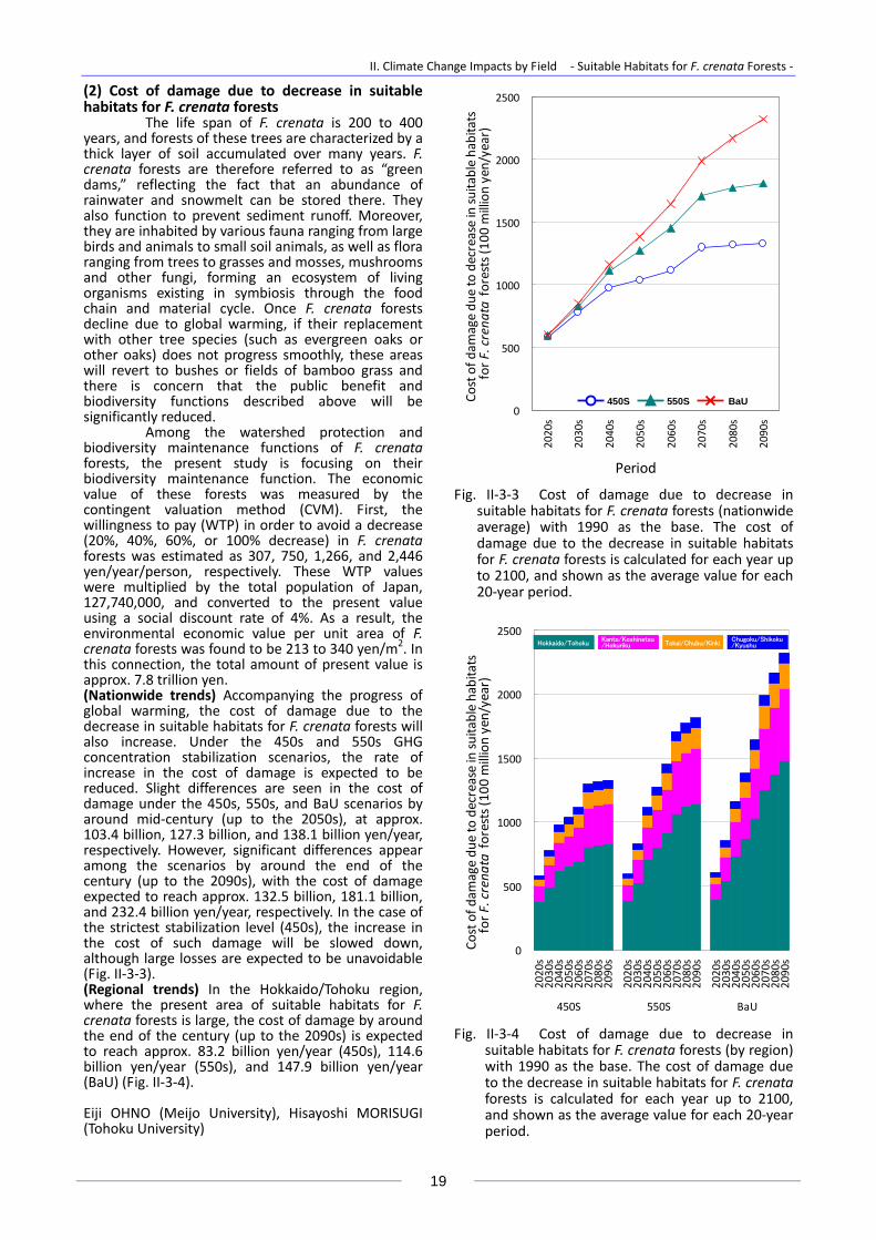
II. Climate Change Impacts by Field ‐ Suitable Habitats for F. crenata Forests ‐
19
(2) Cost of damage due to decrease in suitable habitats for F. crenata forests
The life span of F. crenata is 200 to 400 years, and forests of these trees are characterized by a thick layer of soil accumulated over many years. F. crenata forests are therefore referred to as “green dams,” reflecting the fact that an abundance of rainwater and snowmelt can be stored there. They also function to prevent sediment runoff. Moreover, they are inhabited by various fauna ranging from large birds and animals to small soil animals, as well as flora ranging from trees to grasses and mosses, mushrooms and other fungi, forming an ecosystem of living organisms existing in symbiosis through the food chain and material cycle. Once F. crenata forests decline due to global warming, if their replacement with other tree species (such as evergreen oaks or other oaks) does not progress smoothly, these areas will revert to bushes or fields of bamboo grass and there is concern that the public benefit and biodiversity functions described above will be significantly reduced.
Among the watershed protection and biodiversity maintenance functions of F. crenata forests, the present study is focusing on their biodiversity maintenance function. The economic value of these forests was measured by the contingent valuation method (CVM). First, the willingness to pay (WTP) in order to avoid a decrease (20%, 40%, 60%, or 100% decrease) in F. crenata forests was estimated as 307, 750, 1,266, and 2,446 yen/year/person, respectively. These WTP values were multiplied by the total population of Japan, 127,740,000, and converted to the present value using a social discount rate of 4%. As a result, the environmental economic value per unit area of F. crenata forests was found to be 213 to 340 yen/m2. In this connection, the total amount of present value is approx. 7.8 trillion yen. (Nationwide trends) Accompanying the progress of global warming, the cost of damage due to the decrease in suitable habitats for F. crenata forests will also increase. Under the 450s and 550s GHG concentration stabilization scenarios, the rate of increase in the cost of damage is expected to be reduced. Slight differences are seen in the cost of damage under the 450s, 550s, and BaU scenarios by around mid‐century (up to the 2050s), at approx. 103.4 billion, 127.3 billion, and 138.1 billion yen/year, respectively. However, significant differences appear among the scenarios by around the end of the century (up to the 2090s), with the cost of damage expected to reach approx. 132.5 billion, 181.1 billion, and 232.4 billion yen/year, respectively. In the case of the strictest stabilization level (450s), the increase in the cost of such damage will be slowed down, although large losses are expected to be unavoidable (Fig. II‐3‐3). (Regional trends) In the Hokkaido/Tohoku region, where the present area of suitable habitats for F. crenata forests is large, the cost of damage by around the end of the century (up to the 2090s) is expected to reach approx. 83.2 billion yen/year (450s), 114.6 billion yen/year (550s), and 147.9 billion yen/year (BaU) (Fig. II‐3‐4). Eiji OHNO (Meijo University), Hisayoshi MORISUGI (Tohoku University)
0
500
1000
1500
2000
2500
2020s
2030s
2040s
2050s
2060s
2070s
2080s
2090s
PeriodCo
st of d
amage du
e to decrease in suitable habitats
for F. crena
ta forests (1
00 million yen/year)
Fig. II‐3‐3 Cost of damage due to decrease in
suitable habitats for F. crenata forests (nationwide average) with 1990 as the base. The cost of damage due to the decrease in suitable habitats for F. crenata forests is calculated for each year up to 2100, and shown as the average value for each 20‐year period.
0
500
1000
1500
2000
2500
2020s
2030s
2040s
2050s
2060s
2070s
2080s
2090s
2020s
2030s
2040s
2050s
2060s
2070s
2080s
2090s
2020s
2030s
2040s
2050s
2060s
2070s
2080s
2090s
450S 550S BaU
Cost of d
amage du
e to decrease in suitable habitats
for F. crena
ta fo
rests (100
million yen/year)
Fig. II‐3‐4 Cost of damage due to decrease in
suitable habitats for F. crenata forests (by region) with 1990 as the base. The cost of damage due to the decrease in suitable habitats for F. crenata forests is calculated for each year up to 2100, and shown as the average value for each 20‐year period.
450S 550S BaU
Chugoku/Shikoku/KyushuTokai/Chubu/Kinki
Kanto/Koshinetsu/HokurikuHokkaido/Tohoku
Chugoku/Shikoku/KyushuTokai/Chubu/Kinki
Kanto/Koshinetsu/HokurikuHokkaido/Tohoku

II. Climate Change Impacts by Field ‐ Areas at Risk of Pine Wilt ‐
20
4. Areas at Risk of Pine Wilt
4.1 Estimation Method (1) Outline of model
Based on the mesh climatic data, zoning of the risks of pine wilt under the conditions of global warming was performed taking the forms of land use into account.
Based on the temperature data (mean value over the 30 years from 1971 to 2000) of the mesh climatic data 2000, the temperature environment for every 1°C increase in monthly mean temperature was calculated for each mesh cell. Then, based on the Third Mesh Vegetation Database (MVDB) of the Vegetation Survey conducted as part of the Fifth National Survey on the Natural Environment (NSNE) by the Ministry of the Environment, areas currently forested either in a natural state or under forestry management that are considered to have the possibility of becoming areas of pine forest depending on the temperature conditions and composition of tree types were demarcated (hereafter referred to as “potential pine forest areas”). The risk of pine wilt under the conditions of global warming was obtained for these potential pine forest areas, the results were mapped, and impact functions were developed by prefecture.
The risk of pine wilt was assessed using the MB index, a type of climatic data proposed by Taketani et al. (1975). The MB index is a summation of the mean temperature of each month in a year, with a threshold of 15°C. This is obtained by subtracting 15°C from the mean temperature of each month having a mean temperature of 15°C or more, and totaling these values. The relationship of the MB index with the actual conditions of damage in various locations has been classified as follows: areas with an MB index of more than 22 are at high risk of pine wilt (zone 3), areas with an MB index of less than 19 are naturally suppressed areas where the appearance of pine wilt is suppressed by temperature (zone 1), and areas with an MB index of 19‐22 are naturally suppressed boundary areas at the boundary of these two areas (zone 2) (Nakamura, 2006). In the present study also, zone numbers according to these classifications based on the MB index were assigned in each third‐mesh cell.
Data by prefecture were prepared based on the nationwide municipal boundary data of ESRI Japan Corporation. By superimposing the polygon data by prefecture and the third‐mesh data, the third‐mesh data containing the center of balance in the polygon of each prefecture were extracted and an impact function was prepared. These impact functions by prefecture contain the values calculated from the
ratio of points classified as risk zone 3 to all third‐mesh points with the exception of areas excluded due to land use as specified in the reference material. Reference material: Japanese pine sawyer (Monochamus alternatus) (top) and pinewood nematode (Bursaphelenchus xylophilus) (bottom), which cause of pine wilt
(Photos by Forestry and Forest Products Research Institute) (2) References 1) Taketani A, Okuda M, and Hosoda R (1975) The meteorological analysis on the epidemic mortality of pine trees, with special reference to the effective accumulated temperature. J. Japanese Forestry Society 57, 169‐175 (in Japanese). 2) Nakamura K and Noguchi E (2006) Estimating the distribution of naturally suppressed area of pine wilt disease epidemic using a thermal index: Renewal of MB index. Proc. 117th Japanese Forest Society Congress, PF16 (CD‐ROM) (in Japanese).

II. Climate Change Impacts by Field ‐ Areas at Risk of Pine Wilt ‐
21
4.2 Future Impacts (1) Areas at risk of pine wilt
Changes in areas at risk of pine wilt were estimated with future changes in annual mean temperature as the climatic variable. Here, the ratio of change in areas of pine distribution from those not at risk of pine wilt to those at risk of pine wilt in the future was estimated with 1990 as the base year. (Nationwide trends) Areas at risk of pine wilt will expand accompanying the progress of global warming. Regardless of the stabilization level, areas at risk are expected to continue to expand in the future. However, under the 450s scenario, in which the GHG concentration is stabilized at the lowest level, there is a possibility that the trend of expansion will be halted around the end of the century.
Slight differences in the areas at risk of pine wilt nationwide under the 450s, 550s, and BaU scenarios are seen by around mid‐century (up to the 2050s), at approx. 22%, 26%, and 28%, respectively. However, significant differences appear among the scenarios by around the end of the century (up to the 2090s), with the areas at risk expected to reach approx. 27%, 37%, and 51%, respectively (Fig. II‐4‐1). (Regional trends) Areas at risk of pine wilt are expected to expand in all regions accompanying the progress of global warming (Fig. II‐4‐2).
With the acceleration of pine wilt damage due to global warming (i.e., decline of pine forests), thinning of forests and increased coverage by vegetation such as bamboo grass or ferns can be expected , leading to concern that the various functions of these forests will be significantly lowered. Such functions of pine forests include their role as forest reserves, which is important in terms of conserving national land (functions of serving as windbreaks, preventing sand movement, and protecting against tides); scenic beauty represented by views of sandy beaches dotted with pine trees, as seen in the Nihon sankei, the three most famous scenic places in Japan; and use of the wood for building materials, civil engineering materials, pulp, the production of matsutake mushrooms, etc. Hiromu DAIMARU and Katsunori NAKAMURA (Forestry and Forest Products Research Institute)
0
10
20
30
40
50
60
2020s
2030s
2040s
2050s
2060s
2070s
2080s
2090s
PeriodRatio
of A
rea at risk of pine wilt (%
)
Fig. II‐4‐1 Ratio of change in areas of pine
distribution from those not at risk of pine wilt to those at risk of pine wilt (nationwide average) with 1990 as the base. The ratio is calculated for each year up to 2100, and shown as the average value for each 20‐year period.
0
5
10
15
20
25
30
2020s
2030s
2040s
2050s
2060s
2070s
2080s
2090s
2020s
2030s
2040s
2050s
2060s
2070s
2080s
2090s
2020s
2030s
2040s
2050s
2060s
2070s
2080s
2090s
450S 550S BaU
Area at risk of p
ine wilt
(%,199
0 = natio
nwide total is 0%
)
Fig. II‐4‐2 Ratio of change in areas of pine distribution
from those not at risk of pine wilt to those at risk of pine wilt (by region) with 1990 as the base. The ratio is calculated for each year up to 2100, and shown as the average value for each 20‐year period.
Chugoku/Shikoku/KyushuTokai/Chubu/Kinki
Kanto/Koshinetsu/HokurikuHokkaido/Tohoku
Chugoku/Shikoku/KyushuTokai/Chubu/Kinki
Kanto/Koshinetsu/HokurikuHokkaido/Tohoku

II. Climate Change Impacts by Field ‐ Rice Yield ‐
22
5. Rice Yield
5.1 Estimation Method (1) Outline of model
The model used for rice yield projection has the same structure as the model of Horie et al. (1995), and consists of three submodels: (1) a projection model, which projects the growth stage from seeding, heading, and flowering, through to pollination and harvesting; (2) a biomass production model, which describes the development of leaf area as well as the process of production of assimilation products by photosynthesis; and (3) a grain formation model, which describes the processes of fertility and ripening.
Projection models for crop growth and yield are generally applied to studies targeting phenomena on the cultivated field scale, and the parameters of the model are determined for each variety and each region. Implementation of such a model thus requires detailed information on varieties, cultivation management, etc., making it unsuitable for assessing the whole of Japan on a broad scale. Therefore, in order to reflect the growth condition of rice plants, annual changes in rice yield, differences in environmental conditions among regions, etc., as well as to apply the model on a broad scale, the parameters of the model were determined for each prefecture. The procedure used is described below. 1) The paddy field distribution in the targeted
prefecture is extracted using the digital national land information (1 km x 1 km grid).
2) The average weather factors (maximum and minimum temperatures and insolation, by day) are calculated for the paddy field grid extracted in step 1, using AMeDAS mesh weather data. Although atmospheric CO2 concentration changes with time, it is assumed to be uniform nationwide.
3) With the 25 years from 1979 to 2003 as the targeted period, the prefectural average weather factors prepared in step 2 are input into the model, while making comparisons with time series data of the average transplanting date, average heading date, average harvesting date, and yield using agriculture and forestry statistics by prefecture nationwide to estimate the parameters of the model by Bayesian estimation. It should be noted here that estimation of the parameters was carried out using data of odd‐numbered years within the target period, while verification of the model was carried out for all years including even‐numbered years. Among the total of 32 parameters contained in the model, 13 were determined using the above method.
The remaining parameter values were extracted from existing studies, and are related to rice plant characteristics that are independent of the characteristics of varieties and the conditions of management.
The Process‐based Regional‐Scale Rice Yield Simulator with Bayesian Inference (PRYSBI; Iizumi et al., 2009), a mechanistic model for wide‐area projection of rice yields prepared using the above method, statistically reflects past actual variety characteristics and changes in yield, although in terms of prefectural averages, and also incorporates the mechanism of the environmental responses of crops. Moreover, it is possible to quantitatively reproduce interannual variations in yields by taking the average of the parameter ensemble calculated by varying sets of parameter values based on posterior distributions of parameters contained in the model obtained by Bayesian estimation. The results of comparisons between estimated and statistical values of rice yields obtained by PRYSBI have verified that interannual variations in yields divided into the four regional blocks of Hokkaido/Tohoku, Kanto/Koshinetsu/Hokuriku, Tokai/Chubu/Kinki, and Chugoku/Shikoku/Kyushu are properly reproduced using the average of the parameter ensemble members. It is possible to estimate the heading date with an accuracy of within three days and the yield with an accuracy of within 0.2 t/ha in terms of the nationwide average. (2) References 1) Horie T, Nakagawa H, Centeno HGS, and Kropff M (1995) The
rice crop simulation model SIMRIW and its testing, In: Modeling the impact of climate change on rice in Asia, Matthews RB et al. (eds.). CAB International, Oxon, 51‐66.
2) Iizumi T, Yokozawa M, and Nishimori M (2009) Parameter estimation and uncertainty analysis of a large‐scale crop model for paddy rice: Application of a Bayesian approach. Agric. and Forest Meteorology 149, 333‐348.

II. Climate Change Impacts by Field ‐ Rice Yield ‐
23
5.2 Future Impacts (1) Rice yield
Future rice yields were estimated with changes in accumulated insolation in the warm season (May‐October), mean temperature change in summer (July, August), and mean temperature change and CO2 concentration in the warm season excluding summer (May, June, September, October) as climatic variables. Here, adaptation measures have not been taken into consideration.
The impacts of climate change can be interpreted as follows. Assuming no change in insolation, the biomass (weight of paddy rice) is determined by the trade‐off between the decrease accompanying the reduction in the growth period due to temperature rise and the increase accompanying the CO2 fertilization effect. Moreover, the positive effect due to the reduction in cold weather damage in currently cool regions, and the negative effect due to high‐temperature‐induced sterility in currently warm regions, are added to the effect of the ripening period, and the final rice yield is determined. (Nationwide trends) Until around mid‐century (up to the 2050s), increases in yield are seen due to the effect of the reduction in growth period being less than the CO2 fertilization effect, and also as a result of the reduction in cold weather damage. Thereafter, under the 450s and 550s scenarios, the trend reverses to one of decreasing yields toward the end of the century (up to the 2090s) because of the effect of the reduction in growth period being greater than the CO2 fertilization effect, as well as reductions in yield due to high temperature. Under the BaU scenario, on the other hand, although the trend will not reverse to a reduction in yield, the rate of increase is expected to become gradually lower. (Regional trends) In all regions, the yield increases until the negative effect of temperature rise exceeding the CO2 fertilization effect appears, after which it decreases. The positive effect of temperature rise is especially pronounced in the Hokkaido/Tohoku region, with the result that the year in which the yield reverses to a decreasing trend is later there than in other regions. Under the BaU scenario, yields increase in the Chugoku/Shikoku/Kyushu and Kanto/Koshinetsu/Hokuriku regions due to the CO2 fertilization effect. In the Tokai/Chubu/Kinki region, on the other hand, the temperature will become higher than in other regions due to the effect of the Pacific high‐pressure system (“Pacific high”), and since the flowering stage of rice coincides with the period of high temperature, the trend in yield can be forecast to reverse to a declining trend from 2050 onwards. Under the 450s and 550s scenarios, the trend is expected to reverse to a declining trend after the 2030s.
Hence, an increase in rice yield can be initially expected due to global warming. With further rises in temperature, however, the trend is expected to reverse to a decrease in yield together with a projected increase in interannual variations in yield due to the relationship between temperature and sterility rate (described in the next subsection). Furthermore, there are also concerns regarding the impacts on quality and taste.
Masayuki YOKOZAWA and Toshichika IIZUMI (National Institute for Agro‐Environmental Sciences)
4.8
4.9
5.0
5.1
5.2
2020s
2030s
2040s
2050s
2060s
2070s
2080s
2090s
Period
Rice yield (kg/ha)
Fig. II‐5‐1 Rice yield (nationwide average). The ratio
is calculated for each year up to 2100, and shown as the average value for each 20‐year period.
4.6
4.8
5.0
5.2
5.4
5.6
5.8
6.0
6.2
2020s
2030s
2040s
2050s
2060s
2070s
2080s
2090s
2020s
2030s
2040s
2050s
2060s
2070s
2080s
2090s
2020s
2030s
2040s
2050s
2060s
2070s
2080s
2090s
450S 550S BaU
Rice yield (t/ha)
Fig. II‐5‐2 Rice yield (by region). The ratio is
calculated for each year up to 2100, and shown as the average value for each 20‐year period.
450S 550S BaU
Chugoku/Shikoku/KyushuTokai/Chubu/Kinki
Kanto/Koshinetsu/HokurikuHokkaido/Tohoku
Chugoku/Shikoku/KyushuTokai/Chubu/Kinki
Kanto/Koshinetsu/HokurikuHokkaido/Tohoku

II. Climate Change Impacts by Field ‐ Rice Yield ‐
24
(2) Rice yield variation Since the reproducibility of interannual
variations in yield is low in the integrated assessment model, the regional impacts of variability were analyzed using PRYSBI. Figure II‐5‐3 shows the results of calculations of changes in regional average rice yields with respect to the level of rise of the mean temperature in the warm season (May‐October) for 43 cases of climate change scenarios (including the present climate). The above approach has been adopted because of the use of multiple scenarios of climate change including GHG emission scenarios and the difficulty of comparing impacts annually due to the variations in the progress of climate change according to the scenarios. Therefore, although the x‐axis shows only the mean temperature in the warm season, in actuality the daily temperature and impacts of variations in insolation are included. (Nationwide trends) As can be seen in Fig. II‐5‐3, when the mean temperature in the warm season in Japan and the surrounding area increases by 3°C or more (compared with 1981‐2000), variations in yield increase in all regions. This is due to the response of the high‐temperature‐induced sterility process model described later (Fig. II‐5‐4). (Regional trends) The synoptic field of the climate model reveals that, particularly in the Tokai/Chubu/Kinki region, the Pacific high will be strengthened with climate change and its edge will reach this region, thereby intensifying the high‐temperature trend in summer. This characteristic has already been seen in recent years, and it is possible that it will become a further cause of
decreases in yield and greater amplification of variations in yield in this region in the future.
As shown in Fig. II‐5‐4, the high‐temperature‐induced sterility process shows a rapid increase in sterility taking place due to the occurrence of high‐temperature events (> 35°C) on the scale of a day during the flowering period. Therefore, when the mean temperature increases due to global warming, even with weather changes occurring at about the same level as at present, variations in the sterility rate will be amplified and, by extension, variations in yield are expected to increase. However, this relationship has a large degree of uncertainty due to differences in varieties, cultivation management, etc., so further studies are necessary. Masayuki YOKOZAWA and Toshichika IIZUMI (National Institute for Agro‐Environmental Sciences)
Paddy rice (Japonica )
100
0
80
60
40
20
100
0
80
60
40
20
Paddy rice (Japonica )
100
0
80
60
40
20
100
0
80
60
40
20
Mean value of max. temperature in flowering stage
Present
Under global warming
Ferti
lity
rate
(%)
Ste
rility
rate
(%)
Paddy rice (Japonica )
100
0
80
60
40
20
100
0
80
60
40
20
Paddy rice (Japonica )
100
0
80
60
40
20
100
0
80
60
40
20
Mean value of max. temperature in flowering stage
Present
Under global warming
Ferti
lity
rate
(%)
Ste
rility
rate
(%)
Fig. II‐5‐4 Relationship between temperature at the
flowering stage and sterility rate
Fig. II‐5‐3 Regional average yield (upper figures) and changes in coefficient of variation (lower figures) with
respect to the level of rise of the mean temperature in the warm season (May‐October), using mean values from 1981 to 2000
This analysis is based on multiple future climate projection data reported in the Fourth Assessment Report (AR4) of the IPCC. The climate change scenario data used were the output results for two GHG emission scenarios, namely, the SRES A1B and A2 scenarios, from nine types and eight types of global climate models for the A1B and A2 scenarios, respectively. The level of temperature rise from the present (mean temperature from 1981 to 2000) was used as an index, and its impact was expressed. For the estimation of future yield, data by day in the two periods of 2046‐2065 and 2081‐2100 were used. The spatial resolution of data after linear interpolation is approx. 1 km in the latitudinal and longitudinal directions for MIROC‐hires, and approx. 10 km for the other climate models.
北海道・東北 関東・甲信越・北陸 東海・中部・近畿 中国・四国・九州Hokkaido/Tohoku Kanto/Koshinetsu/Hokuriku Tokai/Chubu/Kinki Chugoku/Shikoku/Kyushu

II. Climate Change Impacts by Field ‐ Sand Beach Loss due to Sea Level Rise ‐
25
6. Sand Beach Loss due to Sea Level Rise
6.1 Estimation Method (1) Outline of model
The total length of Japan’s coastline is 35,236 km, approx. 20% (7,060 km) of which is accounted for by sand beaches. Since olden times, these beaches have been supporting people’s lives as bases for marine transportation as well as locations for fisheries and agriculture. In the present day, their spiritual and cultural value as places for recreational activities such as sea bathing, camping, bird watching, strolling, etc. has also been recognized. That is, not only the market value of sand beaches (value in terms of market economics) but also their nonmarket value (value in terms of environmental economics) has come to be widely recognized.
In the present study, with the aim of providing a basic unit of monetary assessment that is necessary when examining the cost‐effectiveness of measures against global warming in relation to the prevention of sand beach loss, the value of sand beaches that will be lost as a result of sea level rise is measured. Here, among the nonmarket values of sand beaches, their utility value as sea bathing beaches (recreational value) is focused on. The travel cost method (TCM) is adopted as the measurement method.
When applying TCM, the demand function of traffic for sand beach utilization purposes is expressed by the following equation:
( )ijij px ⋅+= βαexp (1)
where ijx is the volume of traffic for sand beach
utilization purposes between regions ji − , pij is the volume of traffic for leisure purposes between regions
ji − , ji − represents the departure site to the
arrival site (prefectures), and βα , are unknown parameters.
In TCM, recreational value is defined by the consumer surplus in the transportation market as the proxy market of the recreational activities concerned. Therefore, the recreational value of sea bathing from sand beaches is assessed by the consumer surplus CS of the demand of traffic for sand beach utilization purposes given by Eq. (1) as follows:
∑∫∞
=ij
p ijijij
dpxCS ∑⋅−=ij
ijxβ1
(2)
In Eq. (2), the consumer surplus in the overall transportation market is expressed as the constant multiple of total traffic volume. From this, the consumer surplus cs of sand beaches per one time of use is given by the following equation:
β1
−==∑
ijijx
CScs (3)
It is seen from Eq. (3) that, irrespective of whether a person lives close to or far from a sand beach, or whether a person uses sand beaches many times or occasionally, the consumer surplus per sand beach per one time of use is constant. This means that when totaling the recreational value of the use of sand beaches, it is only necessary to count the number of visitors to the sand beach concerned and there is no need to identify where the visitors came from.
Through the parameter estimation shown in Eq. (1), the basic unit of sand beach utility value (recreational value) can be obtained from Eq. (3). By multiplying the number of annual users of sand beaches (for sea bathing) nationwide by this basic unit, the annual recreational value of sand beaches nationwide can be obtained. Moreover, by converting this annual recreational value to present value using a social discount rate (4% per year), and dividing this value by the area of sand beaches nationwide (191.1 km2), the recreational value per unit area of sand beach can be obtained. This value becomes the basic unit of monetary assessment for sand beaches. By multiplying the area of sand beach loss due to sea level rise by this basic unit, the loss of value due to sea level rise can be measured.
Due to the sea level rise accompanying global warming in recent years, sand beaches having the value described above are facing a crisis of disappearance. Projections by Mimura et al. (1994) with regard to sand beaches in Japan (total area 191 km2) show that sea level rises of 30 cm, 65 cm, and 100 cm will result in the disappearance of 108 km2 (56.6%), 156 km2 (81.7%), and 173 km2 (90.3%) of sand beaches, respectively.
(2) References 1) Ohno E, Hayashiyama Y, Morisugi H, and Nohara K (2009)
Economic assessment of sand beach disappearance due to global warming: Approach using the travel cost method. Chikyu Kankyo 14,291‐297 (in Japanese).
2) Mimura N, Inoue K, Kiyohashi S, Izumiya T, and Nobuoka H (1994) Impact assessment of sea level rise on sandy beaches (2): Verification of validity of projection model and nationwide scale assessment. J. Coastal Engineering 41, 1161‐1165 (in Japanese).

II. Climate Change Impacts by Field ‐ Sand Beach Loss due to Sea Level Rise ‐
26
6.2 Future Impacts (1) Cost of damage due to sand beach loss
The relationships between sea level rises and areas of encroachment were obtained based on the research results of Mimura et al. (1994), and the areas of beaches encroached on for given future sea level rises were estimated by prefecture. Here, the area of sand beach loss in the base year (1990) is assumed to be zero. Differences in sea level rises among regions are not taken into consideration and it is assumed that sea level changes occur uniformly throughout Japan; adaptation measures are also not taken into consideration.
Even if the atmosphere reaches an equilibrium temperature, seawater temperature rise accompanied by the resultant sea level rise will continue for a prolonged period. Moreover, over the long term, sea level rise due to melting of the Greenland ice sheet is also a source of concern. Therefore, the encroachment of sand beaches due to sea level rise will be a long‐lasting phenomenon during the 21st century and beyond, and it is necessary to pay attention to the possibility of significant damage to the disaster prevention function of sand beaches as well as to their ecosystems.
In the present study, first the recreational value of sand beaches was measured by TCM. From the results, it was estimated that the value of sand beaches per one time of use is 2,179 yen/time, amounting to 92.2 billion yen/year nationwide (present value: 2,304.6 billion yen). Dividing the nationwide value of sand beaches by the nationwide area of sand beaches (191.1 km2), the basic unit of monetary assessment for sand beaches becomes 12,058 yen/m2 as the nationwide average. The estimated sea level rises in the 2090s according to the scenarios used in this study are 0.15 m (450s), 0.19 m (550s), and 0.24 m (BaU). Moreover, according to the Fourth Assessment Report (AR4) of the IPCC, there are cases in which the sea level rise by the end of the century may become double these figures or more.
Even under the 450s scenario, in which the GHG stabilization concentration is lowest, the area of sand beach loss due to sea level rise continues to increase until around the end of the century (up to the 2090s), with approx. 29% of the area of sand beaches expected to be lost. On the other hand, under the 550s and BaU scenarios, approx. 37% and 47%, respectively, of the area is expected to be lost during the same period.
The cost of damage due to sand beach loss by around the end of the century (up to the 2090s) is expected to reach approx. 27.3 billion yen/year (450s), 33.8 billion yen/year (550s), and 43.0 billion yen/year (BaU). When compared with BaU, a substantial damage reduction effect can be expected under the 450s scenario. However, damage due to the rise in sea level is expected to continue for a long period, including under the 450s scenario, so adaptation measures from the long‐term viewpoint are
important. Eiji OHNO (Meijo University), Hisayoshi MORISUGI and Yasuhisa HAYASHIYAMA (Tohoku University)
0
10
20
30
40
50
2020s
2030s
2040s
2050s
2060s
2070s
2080s
2090s
Period
Ratio of area of sand beach loss (%
)
Fig. II‐6‐1 Ratio of sand beach loss (nationwide
average). The ratio is calculated for each year up to 2100, and shown as the average value for each 20‐year period.
0
100
200
300
400
500
2020s
2030s
2040s
2050s
2060s
2070s
2080s
2090s
Period
Cost of d
amage du
e to sand beach loss
(100
million yen/year)
Fig. II‐6‐2 Cost of damage due to sand beach loss
(nationwide average). The ratio is calculated for each year up to 2100, and shown as the average value for each 20‐year period.
450S 550S BaU
450S 550S BaU
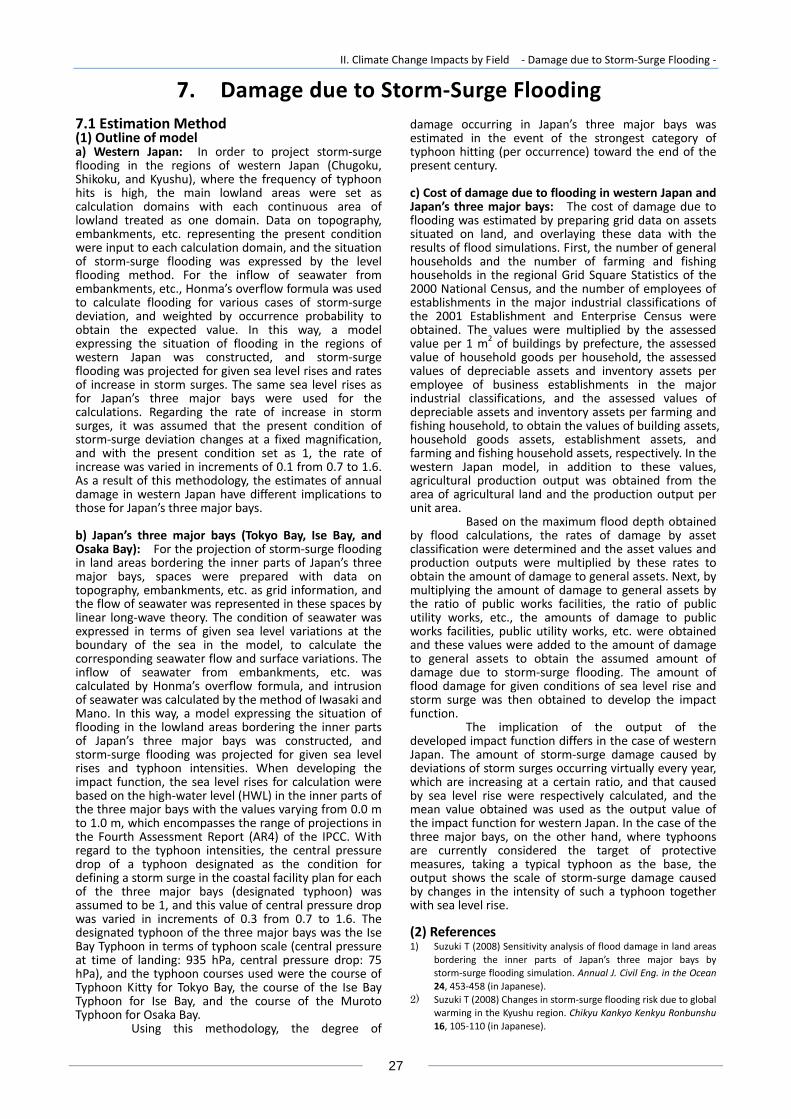
II. Climate Change Impacts by Field ‐ Damage due to Storm‐Surge Flooding ‐
27
7. Damage due to Storm‐Surge Flooding
7.1 Estimation Method (1) Outline of model a) Western Japan: In order to project storm‐surge flooding in the regions of western Japan (Chugoku, Shikoku, and Kyushu), where the frequency of typhoon hits is high, the main lowland areas were set as calculation domains with each continuous area of lowland treated as one domain. Data on topography, embankments, etc. representing the present condition were input to each calculation domain, and the situation of storm‐surge flooding was expressed by the level flooding method. For the inflow of seawater from embankments, etc., Honma’s overflow formula was used to calculate flooding for various cases of storm‐surge deviation, and weighted by occurrence probability to obtain the expected value. In this way, a model expressing the situation of flooding in the regions of western Japan was constructed, and storm‐surge flooding was projected for given sea level rises and rates of increase in storm surges. The same sea level rises as for Japan’s three major bays were used for the calculations. Regarding the rate of increase in storm surges, it was assumed that the present condition of storm‐surge deviation changes at a fixed magnification, and with the present condition set as 1, the rate of increase was varied in increments of 0.1 from 0.7 to 1.6. As a result of this methodology, the estimates of annual damage in western Japan have different implications to those for Japan’s three major bays. b) Japan’s three major bays (Tokyo Bay, Ise Bay, and Osaka Bay): For the projection of storm‐surge flooding in land areas bordering the inner parts of Japan’s three major bays, spaces were prepared with data on topography, embankments, etc. as grid information, and the flow of seawater was represented in these spaces by linear long‐wave theory. The condition of seawater was expressed in terms of given sea level variations at the boundary of the sea in the model, to calculate the corresponding seawater flow and surface variations. The inflow of seawater from embankments, etc. was calculated by Honma’s overflow formula, and intrusion of seawater was calculated by the method of Iwasaki and Mano. In this way, a model expressing the situation of flooding in the lowland areas bordering the inner parts of Japan’s three major bays was constructed, and storm‐surge flooding was projected for given sea level rises and typhoon intensities. When developing the impact function, the sea level rises for calculation were based on the high‐water level (HWL) in the inner parts of the three major bays with the values varying from 0.0 m to 1.0 m, which encompasses the range of projections in the Fourth Assessment Report (AR4) of the IPCC. With regard to the typhoon intensities, the central pressure drop of a typhoon designated as the condition for defining a storm surge in the coastal facility plan for each of the three major bays (designated typhoon) was assumed to be 1, and this value of central pressure drop was varied in increments of 0.3 from 0.7 to 1.6. The designated typhoon of the three major bays was the Ise Bay Typhoon in terms of typhoon scale (central pressure at time of landing: 935 hPa, central pressure drop: 75 hPa), and the typhoon courses used were the course of Typhoon Kitty for Tokyo Bay, the course of the Ise Bay Typhoon for Ise Bay, and the course of the Muroto Typhoon for Osaka Bay.
Using this methodology, the degree of
damage occurring in Japan’s three major bays was estimated in the event of the strongest category of typhoon hitting (per occurrence) toward the end of the present century. c) Cost of damage due to flooding in western Japan and Japan’s three major bays: The cost of damage due to flooding was estimated by preparing grid data on assets situated on land, and overlaying these data with the results of flood simulations. First, the number of general households and the number of farming and fishing households in the regional Grid Square Statistics of the 2000 National Census, and the number of employees of establishments in the major industrial classifications of the 2001 Establishment and Enterprise Census were obtained. The values were multiplied by the assessed value per 1 m2 of buildings by prefecture, the assessed value of household goods per household, the assessed values of depreciable assets and inventory assets per employee of business establishments in the major industrial classifications, and the assessed values of depreciable assets and inventory assets per farming and fishing household, to obtain the values of building assets, household goods assets, establishment assets, and farming and fishing household assets, respectively. In the western Japan model, in addition to these values, agricultural production output was obtained from the area of agricultural land and the production output per unit area.
Based on the maximum flood depth obtained by flood calculations, the rates of damage by asset classification were determined and the asset values and production outputs were multiplied by these rates to obtain the amount of damage to general assets. Next, by multiplying the amount of damage to general assets by the ratio of public works facilities, the ratio of public utility works, etc., the amounts of damage to public works facilities, public utility works, etc. were obtained and these values were added to the amount of damage to general assets to obtain the assumed amount of damage due to storm‐surge flooding. The amount of flood damage for given conditions of sea level rise and storm surge was then obtained to develop the impact function.
The implication of the output of the developed impact function differs in the case of western Japan. The amount of storm‐surge damage caused by deviations of storm surges occurring virtually every year, which are increasing at a certain ratio, and that caused by sea level rise were respectively calculated, and the mean value obtained was used as the output value of the impact function for western Japan. In the case of the three major bays, on the other hand, where typhoons are currently considered the target of protective measures, taking a typical typhoon as the base, the output shows the scale of storm‐surge damage caused by changes in the intensity of such a typhoon together with sea level rise. (2) References 1) Suzuki T (2008) Sensitivity analysis of flood damage in land areas
bordering the inner parts of Japan’s three major bays by storm‐surge flooding simulation. Annual J. Civil Eng. in the Ocean 24, 453‐458 (in Japanese).
2) Suzuki T (2008) Changes in storm‐surge flooding risk due to global warming in the Kyushu region. Chikyu Kankyo Kenkyu Ronbunshu 16, 105‐110 (in Japanese).
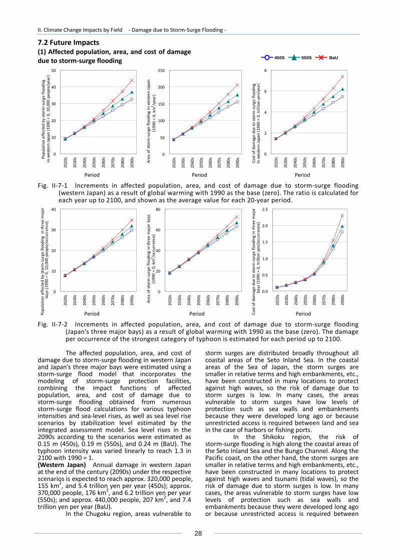
II. Climate Change Impacts by Field ‐ Damage due to Storm‐Surge Flooding ‐
28
7.2 Future Impacts (1) Affected population, area, and cost of damage due to storm‐surge flooding
0
10
20
30
40
502020s
2030s
2040s
2050s
2060s
2070s
2080s
2090s
Period
Populatio
n affected
by storm‐surge
flooding
in western Ja
pan (1990 = 0, 10,000 people/year)
0
50
100
150
200
250
2020s
2030s
2040s
2050s
2060s
2070s
2080s
2090s
Period
Area
of storm
‐surge
flooding
in western Ja
pan
(1990 = 0, km
2 /year)
0
2
4
6
8
2020s
2030s
2040s
2050s
2060s
2070s
2080s
2090s
Period
Cost of d
amage due to storm
‐surge
flooding
in western Ja
pan (1990 = 0, trillion yen/year)
Fig. II‐7‐1 Increments in affected population, area, and cost of damage due to storm‐surge flooding
(western Japan) as a result of global warming with 1990 as the base (zero). The ratio is calculated for each year up to 2100, and shown as the average value for each 20‐year period.
0
10
20
30
40
2020s
2030s
2040s
2050s
2060s
2070s
2080s
2090s
Period
bays (1
990 = 0, 10,000 people/occurrence)
Populatio
n affected
by storm‐surge
flooding
in three major
0
20
40
60
80
2020s
2030s
2040s
2050s
2060s
2070s
2080s
2090s
Period
(1990 = 0, km
2 /occurrence)
Area
of storm
‐surge
flooding
in th
ree major bays
0.0
0.5
1.0
1.5
2.0
2.5
2020s
2030s
2040s
2050s
2060s
2070s
2080s
2090s
Period
bays (1
990 = 0, trillion yen/occurrence)
Cost of d
amage due to storm
‐surge
flooding
in th
ree major
Fig. II‐7‐2 Increments in affected population, area, and cost of damage due to storm‐surge flooding
(Japan’s three major bays) as a result of global warming with 1990 as the base (zero). The damage per occurrence of the strongest category of typhoon is estimated for each period up to 2100.
The affected population, area, and cost of
damage due to storm‐surge flooding in western Japan and Japan’s three major bays were estimated using a storm‐surge flood model that incorporates the modeling of storm‐surge protection facilities, combining the impact functions of affected population, area, and cost of damage due to storm‐surge flooding obtained from numerous storm‐surge flood calculations for various typhoon intensities and sea‐level rises, as well as sea level rise scenarios by stabilization level estimated by the integrated assessment model. Sea level rises in the 2090s according to the scenarios were estimated as 0.15 m (450s), 0.19 m (550s), and 0.24 m (BaU). The typhoon intensity was varied linearly to reach 1.3 in 2100 with 1990 = 1. (Western Japan) Annual damage in western Japan at the end of the century (2090s) under the respective scenarios is expected to reach approx. 320,000 people, 155 km2, and 5.4 trillion yen per year (450s); approx. 370,000 people, 176 km2, and 6.2 trillion yen per year (550s); and approx. 440,000 people, 207 km2, and 7.4 trillion yen per year (BaU).
In the Chugoku region, areas vulnerable to
storm surges are distributed broadly throughout all coastal areas of the Seto Inland Sea. In the coastal areas of the Sea of Japan, the storm surges are smaller in relative terms and high embankments, etc., have been constructed in many locations to protect against high waves, so the risk of damage due to storm surges is low. In many cases, the areas vulnerable to storm surges have low levels of protection such as sea walls and embankments because they were developed long ago or because unrestricted access is required between land and sea in the case of harbors or fishing ports.
In the Shikoku region, the risk of storm‐surge flooding is high along the coastal areas of the Seto Inland Sea and the Bungo Channel. Along the Pacific coast, on the other hand, the storm surges are smaller in relative terms and high embankments, etc., have been constructed in many locations to protect against high waves and tsunami (tidal waves), so the risk of damage due to storm surges is low. In many cases, the areas vulnerable to storm surges have low levels of protection such as sea walls and embankments because they were developed long ago or because unrestricted access is required between
450S 550S BaU

II. Climate Change Impacts by Field ‐ Damage due to Storm‐Surge Flooding ‐
29
land and sea in the case of harbors or fishing ports. In the Kyushu region, there are areas
vulnerable to storm surges in northwestern Kyushu, Kitakyushu, the Suo‐nada Sea, Beppu Bay, the southern part of Miyazaki Prefecture, and the Satsuma Peninsula. This regional distribution is mainly due to the existence of scattered sections with a low level of development of embankments and seawalls. Since Kyushu is a region with a high frequency of typhoon visits, studies are necessary on measures that combine early preparations and long‐term efforts. (Japan’s three major bays) Damage at the time of storm‐surge flooding in Japan’s three major bays at the end of the century (2090s) under the respective scenarios is expected to reach approx. 300,000 people, 63 km2, and 1.8 trillion yen per occurrence (450s); approx. 320,000 people, 67 km2, and 2.0 trillion yen per occurrence (550s); and approx. 350,000 people, 72 km2, and 2.3 trillion yen per occurrence (BaU).
In the inner part of Tokyo Bay along the eastern areas of the Tokyo shoreline, zero‐meter zones extend around the Arakawa and Edogawa rivers. However, the level of protection such as seawalls, floodgates, etc. to protect these lowlands is comparatively high, with the result that not many vulnerable areas are seen there. In contrast, many areas vulnerable to storm surges are seen in the southern coastal areas of Tokyo.
Looking next at the inner part of Ise Bay, zero‐meter zones are widely distributed from the areas surrounding the Kiso Three Rivers to the
environs of Nagoya Port, although areas vulnerable to storm surges are limited to those along the estuaries of the Kiso Three Rivers and the area around the inner part of Nagoya Port. In particular, the depth of flooding is expected to be large on the reclaimed land of Nagoya Port, which was developed a comparatively long time ago, and the surrounding areas. Along the inner part of Osaka Bay, zero‐meter zones extend from the northern to the central areas of Osaka behind the reclaimed land forming the littoral. However, with the progressive development of embankments and floodgates, not many of these areas are vulnerable to storm surges. On the other hand, many areas vulnerable to storm surges are seen on the reclaimed land extending from the central to the southern parts of Osaka Port and its surroundings.
Since the rise in sea level accompanying global warming will continue for a long period, damage will increase over the long term. A long period will also be required for the effects of climate stabilization to appear. Therefore, in order to prevent major damage and avoid the imposition of a larger burden on those implementing the necessary measures, it would be a rational approach to gradually take appropriate measures in line with the degree of progress of global warming. Takeshi SUZUKI (National Institute for Land and Infrastructure Management)
a. Tokyo Bay b. Ise Bay c. Osaka Bay Fig. II‐7‐3 Depth of flood due to storm surge in the case of a 60 cm sea level rise and typhoon intensity
of 1.3 in Japan’s three major bays
a. Chugoku region b. Shikoku region c. Kyushu region Fig. II‐7‐4 Areas of storm‐surge flooding in the case of a 60 cm sea level rise and rate of increase in
storm surges of 1.3 in western Japan
Terrestrial areas
Lowlands
Areas of flooding
Terrestrial areas
Lowlands
Areas of flooding
Terrestrial areas
Lowlands
Areas of flooding

II. Climate Change Impacts by Field ‐ Heat Stress Mortality Risk ‐
30
8. Heat Stress Mortality Risk
8.1 Estimation Method (1) Model for estimating mortality due to heat stress
Mortality due to heat stress refers to death resulting from the reaction of a living body to the harmful stimulus of heat. Specifically, this means mortality due to heatstroke (heat exhaustion, heat cramps, sunstroke), or heart failure in people with cardio respiratory diseases or people of advanced age with lowered reserve capacity of the cardio respiratory system due to dehydration by perspiration, etc.
Mortality due to heat stress in the present study refers to the risk of mortality that is assumed to occur in relation to high temperature. It is quantitatively expressed in terms of the difference between the mortality rate on hot days and that on days of optimal temperature. The relationship between temperature and mortality is expressed on a graph by plotting the daily maximum temperature on the x‐axis and the total mortality rate on the corresponding day on the y‐axis, and performing approximation using a smoothing spline function with six degrees of freedom. As a result, a V‐shaped mortality curve is obtained. The temperature at which this V‐shaped mortality curve is lowest is referred to as the optimal temperature. The optimal temperature was calculated by prefecture in the present study.
Since the mortality rate is lowest at the optimal temperature, which can be considered the point at which temperature is best controlled, deaths in excess of this minimum value due to temperatures higher than the optimal temperature are defined as the mortality due to heat stress.
The risk of mortality due to heat stress is not so high at temperatures close to the optimal temperature, but increases as the temperature becomes further from the optimal temperature. The relative risk of high temperature with the mortality rate at the optimal temperature as the base does not follow a simple linear regression, and an estimation method is required that is not easily affected by the occurrence of a few days of extremely high temperature. Therefore, the method used in the present study broadly divides the temperatures into two categories: exceeding the optimal temperature by less than +5°C, and exceeding the optimal temperature by +5°C or more. The average relative risk in the respective categories was obtained for all prefectures. The following assumptions were made in the future estimations: (a) The population size and structure as well as the
disease structure and mortality rates by cause of
death remain unchanged. (b) The optimal temperature is determined by the
present climate and remains unchanged in the future as well.
(c) Adaptation is not taken into consideration. (2) Outline of economic assessment model for damage due to heat stress (heatstroke)
In order to determine the basic unit of monetary assessment necessary for studying cost‐effectiveness in the prevention of damage due to heat stress as a measure against global warming, the willingness to pay (WTP) and value of statistical life (VSL) for avoiding damage due to heat stress were estimated by the contingent valuation method (CVM). The risk of mortality due to heatstroke, which is the main factor in heat stress, was selected as the sole target of assessment.
In mid‐May 2008, a contingent valuation survey using the Internet was conducted targeting adult males and females nationwide. Among the topics dealt with in this questionnaire survey, entitled “Survey on Attitudes toward Global Warming Issues,” were the following:
Question 1: Degree of concern regarding global warming issues
Question 2: Degree of concern regarding the increase of heatstroke due to global warming
Question 3: WTP in order to avoid increases in the number of heatstroke cases
Question 4: WTP in order to avoid increases in mortality due to heatstroke
Here, the question format was multiple‐bound dichotomous choice, the method of payment was specified as burden sharing, the form of payment as annual payment, and the payment unit as an individual person. (3) References 1) Takahashi K, Honda Y, and Emori S (2007) Assessing Mortality Risk
from Heat Stress due to Global Warming. J. Risk Research 10, 339‐354.
2) Ohno E, Hayashiyama Y, Morisugi H, and Nohara K (2009) Economic assessment of damage of heatstroke due to global warming: Measurement: of VSH and VSL. Chikyu Kankyo Kenkyu Ronbunshu 17 (in press) (in Japanese).

II. Climate Change Impacts by Field ‐ Heat Stress Mortality Risk ‐
31
8.2 Future Impacts (1) Heat stress mortality risk
From the model for estimating mortality due to heat stress and changes in the distribution of temperatures exceeding the optimal temperature, the probability of a person dying due to heat stress during a year was estimated and the rate of change of this value was compared among the scenarios. The heat stress mortality risk in the base period (1981‐2000) was estimated using the daily maximum temperature data (observed values) during those 20 years. Future heat stress mortality risk was estimated by preparing daily maximum temperature data for the future period concerned, by adding the change in annual mean temperature uniformly (without considering seasonal differences in climate change) to the daily maximum temperature data of the 20 years of the base period. For future population data, the value for 1990 was used with future values remaining unchanged. Population composition was not taken into consideration. Only changes in excess mortality at high temperatures due to temperature rise were examined, and changes in excess mortality at low temperatures were not targeted. It was assumed that adaptation does not occur. (Nationwide trends) The lower the level at which GHG concentration is stabilized, the smaller the heat stress mortality risk becomes. Particularly in the case of the strictest stabilization level (450s), the rate of increase in mortality risk is expected to gradually become lower toward the end of the century. When comparing the heat stress mortality risk under the 450s, 550s, and BaU scenarios, the differences remain comparatively small around mid‐century (2050s), at approx. 1.8 times, 2.1 times, and 2.2 times, respectively. At the end of the century (2090s), however, significant differences are expected according to the stabilization level, reaching approx. 2.1 times, 2.8 times, and 3.7 times, respectively. (Regional trends) At all stabilization levels, the largest change in risk (approx. 7 times under BaU) is expected to occur in the Chugoku/Shikoku/Kyushu region. Although dependent on the targeted group, this change in risk is close to the increase in the lung cancer mortality rate due to smoking about 20 cigarettes a day. According to analysis of the daily maximum temperature data used for the calculation, however, this result is not due to a larger rise of daily maximum temperature in this region compared with other regions, but because the estimated value of heat stress mortality risk during the base period in this region is comparatively small (the optimal temperature is high, and the number of days with a daily maximum temperature exceeding the optimal temperature during the base period is small).
Yasushi HONDA (University of Tsukuba), Kiyoshi TAKAHASHI (National Institute for Environmental Studies)
1.0
1.5
2.0
2.5
3.0
3.5
4.0
2020s
2030s
2040s
2050s
2060s
2070s
2080s
2090s
Period
Heat stress mortality risk (199
0 = 1)
Fig. II‐8‐1 Changes in future heat stress mortality risk (nationwide average) with 1981‐2000 as the base. The ratio is calculated for each year up to 2100, and shown as the average value for each 20‐year period.
1
2
3
4
5
6
7
8
2020s
2030s
2040s
2050s
2060s
2070s
2080s
2090s
2020s
2030s
2040s
2050s
2060s
2070s
2080s
2090s
2020s
2030s
2040s
2050s
2060s
2070s
2080s
2090s
450S 550S BaU
Heat stress m
ortality risk (199
0 = 1)
Fig. II‐8‐2 Changes in future heat stress mortality risk (by region) with 1981‐2000 as the base. The ratio is calculated for each year up to 2100, and shown as the average value for each 20‐year period.
450S 550S BaU
Chugoku/Shikoku/KyushuTokai/Chubu/Kinki
Kanto/Koshinetsu/HokurikuHokkaido/Tohoku
Chugoku/Shikoku/KyushuTokai/Chubu/Kinki
Kanto/Koshinetsu/HokurikuHokkaido/Tohoku

II. Climate Change Impacts by Field ‐ Heat Stress Mortality Risk ‐
32
(2) Cost of damage due to heat stress (heatstroke) mortality
Focusing on the mortality risk due to heatstroke, which is the main factor in heat stress, the cost of damage was measured by CVM in the present study. First, WTP in order to avoid an increase (that is, to maintain the present value) in annual mortality due to heatstroke from 0.3 person per 100,000 population (present value) to 0.6 person, 0.9 person, 1.5 people, and 3.0 people (assumed future values) was estimated as 271, 569, 1,195, and 2,849 yen/year/person respectively. When these values of WTP were divided by the changed portion of the respective mortality risks, a VSL for heat stress (heatstroke) of 90.2 to 105.5 million yen/person was obtained. Medical costs were not taken into consideration here.
According to the Japanese vital statistics, the average mortality due to heatstroke under the present conditions is roughly 400 people/year (although interannual variations are large; for example, 904 deaths from this cause were recorded in 2007). This present value for average mortality was multiplied by changes in future risk estimated by the model for estimating excess mortality due to heat stress to calculate changes in mortality due to heatstroke, and this value was further multiplied by the VSL to obtain the estimated cost of damage due to heat stress (heatstroke) mortality. (Nationwide trends) The lower the level at which GHG concentration is stabilized, the lower the cost of damage due to heat stress (heatstroke) mortality becomes. Particularly in the case of the strictest stabilization level (450s), the cost of such damage is expected to roughly reach a ceiling at approx. 50 billion yen/year. With regard to the nationwide average of the cost of damage under the 450s, 550s, and BaU scenarios, differences in the cost of such damage remain comparatively small around mid‐century (2050s), at approx. 37.3 billion, 48.0 billion, and 52.9 billion yen/year. At the end of the century (2090s), however, significant differences are expected according to the stabilization level, reaching approx. 50.1 billion, 77.5 billion, and 119.2 billion yen/year, respectively. (Regional trends) As described above, the cost of damage due to heat stress (heatstroke) mortality was calculated by the multiplication of three indexes (changes in mortality risk, population, and VSL). The results obtained reveal that the cost of damage is large in the Kanto/Koshinetsu/Hokuriku and Tokai/Chubu/Kinki regions, which have high estimated values of heat stress mortality risk during the base and future periods as well as large populations. The rate of increase in the cost of damage is also expected to become larger in the Chugoku/Shikoku/Kyushu
region, where a high increase in risk is expected. Eiji OHNO (Meijo University), Hisayoshi MORISUGI (Tohoku University)
0
300
600
900
1200
2020s
2030s
2040s
2050s
2060s
2070s
2080s
2090s
Period
Cost of d
amage du
e to heat stress (heatstroke)
mortality (100
million yen/year)
Fig. II‐8‐3 Changes in the future cost of damage due to heat stress (heatstroke) mortality (nationwide average) with 1990 as the base. The ratio is calculated for each year up to 2100, and shown as the average value for each 20‐year period
0
300
600
900
1200
2020s
2030s
2040s
2050s
2060s
2070s
2080s
2090s
2020s
2030s
2040s
2050s
2060s
2070s
2080s
2090s
2020s
2030s
2040s
2050s
2060s
2070s
2080s
2090s
450S 550S BaU
Cost of d
amage du
e to heat stress (heatstroke)
mortality (100
million yen/year)
Fig. II‐8‐4 Changes in the future cost of damage due to heat stress (heatstroke) mortality (by region) with 1990 as the base. The ratio is calculated for each year up to 2100, and shown as the average value for each 20‐year period.
450S 550S BaU
Chugoku/Shikoku/KyushuTokai/Chubu/Kinki
Kanto/Koshinetsu/HokurikuHokkaido/Tohoku
Chugoku/Shikoku/KyushuTokai/Chubu/Kinki
Kanto/Koshinetsu/HokurikuHokkaido/Tohoku

Reference Materials
33
Reference Materials
1. Global‐scale impacts due to mean temperature increase The Contribution of Working Group II (WGII) to the Fourth Assessment Report (AR4) of the IPCC notes that policymakers should pay particular attention to the risks of impacts accompanying climate change because of their magnitude, persistence, and other characteristics, referring to them as “key vulnerabilities” and summarized them in detail under the five categories of global social systems, regional systems, global biological systems, geophysical systems, and extreme events. General conclusions according to the range of increase in future global mean temperature are described below. a) Increase in global mean temperature of 0°C to 2°C
Global mean temperature changes of up to 2°C above 1990‐2000 levels would exacerbate already observed key impacts of anthropogenic climate change (high confidence), and trigger others, such as reduced food security in many low‐latitude nations (medium confidence). At the same time, some systems, such as global agricultural productivity, could benefit (low/medium confidence).
b) Increase in global mean temperature of 2°C to 4°C
Global mean temperature changes of 2 to 4°C above 1990‐2000 levels would result in an increasing number of key impacts at all scales (high confidence), such as widespread loss of biodiversity, decreasing global agricultural productivity, and commitment to widespread deglaciation of Greenland (high confidence) and West Antarctic (medium confidence) ice sheets.
c) Increase in global mean temperature exceeding 4°C
Global mean temperature changes greater than 4°C above 1990‐2000 levels would lead to major increases in vulnerability (very high confidence), exceeding the adaptive capacity of many systems (very high confidence).
It can be seen that when the global mean temperature increases by more than 2°C compared with 1990‐2000 levels, the accompanying impacts in each field intensify, and when the temperature increase exceeds 4°C, the adaptive capacity of many systems is exceeded and destructive impacts may occur. Moreover, although beneficial effects
appear in global agricultural productivity in the case of small increases in temperature, as the temperature increases further these beneficial effects are expected to be gradually negated and to change to adverse impacts. Reference 1) IPCC (2007) Climate Change 2007: Climate Change Impacts,
Adaptation and Vulnerability—Contribution of Working Group II to the Fourth Assessment Report of the Intergovernmental Panel on Climate Change. Cambridge University Press, Cambridge, United Kingdom and New York, NY, USA.
2. Impacts of global warming on the world by field The Contribution of WGII to AR4 of the IPCC summarizes the impacts that may occur in each field according to the magnitude of global mean temperature increase from the levels of 1980 to 1999 (1990 levels), as outlined in Fig. A1. These findings, combined with the climate change projections in the Contribution of Working Group I, can serve as scientific materials for answering questions that are essential to policymakers such as the impacts that will occur if no efforts are made to reduce emissions, or necessary emission reduction paths in order to suppress impacts to below a certain level. The report by WGII concludes that, based on the findings concerning impacts projected in each sector and each region, for increases in global mean temperature of less than 1‐3°C above 1990 levels, some impacts are projected to produce benefits in some places and some sectors, and produce costs in other places and other sectors, while for increases in temperature greater than about 2‐3°C, it is very likely that all regions will experience either declines in net benefits or increases in net costs. However, these conclusions do not mean that increases of about 2‐3°C above 1990 levels are considered to be the dangerous level in all fields. For example, an examination of the impacts individually reveals that, even with a temperature increase of 1°C, increased coral bleaching and increasing species range shifts are projected. Moreover, with a temperature increase of 1‐2°C, although the productivity of some cereals will tend to increase at high latitudes, at low latitudes, particularly in arid tropical regions, the productivity will decrease and the risk of starvation will increase, and the mortality rate due to heat waves will also increase. Even in the case of a

Reference Materials
34
temperature increase not exceeding 2‐3°C, the possibility of occurrence of serious impacts is high in vulnerable ecosystems and vulnerable regions (particularly developing countries).
Reference 1) IPCC (2007) Climate Change 2007: Climate Change Impacts,
Adaptation and Vulnerability—Contribution of Working Group II to the Fourth Assessment Report of the Intergovernmental Panel on Climate Change. Cambridge University Press, Cambridge, United Kingdom and New York, NY, USA.
WATER
Global mean annual temperature change relative to 1980-1999 (℃)2 3 41 5℃
COAST
Increased water availability in moist tropics and high latitudesDecreasing water availability and increasing drought in mid-latitudes and semi-arid low latitudes
1.0 to 2.0 billion 1.1 to 3.2 billion0.4 to 1.7 billion
Additional peoplewith increasedwater stress
Increasing amphibianextinction
About 20 to 30% species at inc-reasingly high risk of extinction
ECOSYSTEMS
Increased coral bleaching Most corals bleached Widespread coral mortality
Major extinctions around the globe
Terrestrial biosphere tends toward a net carbon source, as:~15% ~40% of ecosystems affectedIncreasing species range shifts and wildfire risk
Increased damage from floods and storms
2 to 15 million0 to 3 millionAdditional people at risk of coastal flooding each year
HEALTH
Increasing burden from malnutrition, diarrhoeal, cardio-respiratory and infectious diseases
Increased morbidity and mortality from heatwaves, floods and droughts
Changed distribution of some disease vectors Substantial burden on health services
FOOD
Decreases for some cereals
Increases for some cereals
All cereals decrease
Decreases in some regions
Cropproductivity
Mid to high latitudes
Low latitudes
IPCC(2007)
About 30% loss of coastal wetlands
0
Fig. A1 Global impacts by field as a function of global mean annual temperature change ○ Illustrative examples of global impacts projected for climate changes (and sea level and atmospheric carbon dioxide where relevant) associated with different amounts of increase in global average surface temperature in the 21st century. ○ Arrows indicate impacts continuing with increasing temperature. ○ Entries are placed so that the left‐hand side of the text indicates the approximate onset of a given impact. Note: This figure shows temperature change relative to 1980‐1999; this is different from the temperature change compared with prior to the industrial revolution (the temperature increased by 0.5°C during the period from prior to the industrial revolution to 1990).

Reference Materials
35
3. Potential tipping events that could be triggered by global warming Lenton and Schellnhuber (2007) have cited the following eight potential policy‐relevant tipping elements of the Earth’s system that could be triggered by global warming this century, and described global temperature increases that could become the thresholds of events triggering such changes and their degrees of uncertainty, as shown in Fig. A2. a) Arctic summer sea ice: When the area of sea
ice coverage declines, more radiation is absorbed on the sea surface, which will amplify global warming. The ecosystem of the polar region will also be affected.
b) Greenland ice sheet: As a result of melting of the ice sheet over a period of several hundred to several thousand years, the sea level could rise by 2‐7 m.
c) Boreal forest: Increased water stress, increased peak summer heat stress, increased fire due to drying, etc. could lead to large‐scale dieback of the boreal forests and changes in vegetation.
d) West Antarctic ice sheet: As a result of melting of the ice sheet over a period of several hundred to several thousand years, the sea level could rise by 5 m.
e) Amazon rainforest: Due to regional reductions in precipitation (drying) and the positive feedback of deforestation, dieback of forest may be triggered and impacts such as biodiversity loss could occur.
f) Sahara/Sahel and West African monsoon: Due to the increase in the sea surface temperature
gradient between the northern and southern hemispheres under the conditions of global warming, the West African monsoon may be weakened and, as the result, precipitation in the Sahara/Sahel regions could increase and the area of distribution of vegetation could be expanded.
g) El Niño southern oscillation (ENSO) amplitude: Increased ocean heat uptake could cause a deepening of the thermocline in the East Equatorial Pacific and a consequent shift to greater amplitude/more frequent ENSO. Regarding its impacts, there is concern over intensification and increased frequency of disasters due to extreme weather events such as drought in Southeast Asia, etc.
h) Atlantic meridional overturning circulation: As a result of massive quantities of freshwater from the melting of glaciers and ice sheets flowing into the North Atlantic, and increases in the upper ocean water temperature, a shutoff of thermohaline circulation, which is formed by differences in seawater density, could occur and large‐scale instability of and changes in the global climate system may take place.
References 1) Lenton TM and Schellnhuber HJ (2007) Tipping the scales.
Nature Reports Climate Change 2007.65, Nature Publishing Group.
2) Lenton TM, Hermann H, Kriegler E, Hall JW, Lucht W, Rahmstorf S, and Schellnhuber HJ (2008) Tipping elements in the Earth’s climate system. PNAS 105 (6), 1786‐1793.
Global w
arming above presen
t tem
perature(℃
)
Year 210
0 range (IP
CC 200
7)
Global w
arming above presen
t tem
perature(℃
)
Year 210
0 range (IP
CC 200
7)
Fig. A2 Potential policy‐relevant tipping elements that could be triggered by global warming this century (Potential policy‐relevant tipping elements that could be triggered by global warming this century, with shading indicating their uncertain thresholds. For each threshold, the transition from white to yellow indicates a lower bound of its proximity, and the transition from yellow to red, an upper bound. The degree of uncertainty is represented by the spread of the color transition.)

Reference Materials
36
4. Impacts of global warming on Japan Various studies have been carried out on the impacts of global warming on Japan other than the research conducted under the present project. The results of existing studies are summarized in Fig. A3 in a similar format to Fig. A1. References 1) Daily mean precipitation change: Source (1), p.8, Fig. 1. 2) Change in rice yield: Source (1), p.79, Fig. I‐VI‐2. 3) Change in distribution of suitable lands for apple and
mandarin orange cultivation: Source (2), pp.97 and 102; Sugiura and Yokozawa (2004) Impact of Global Warming on Environments for Apple and Satsuma Mandarin Production Estimated from Changes in the Annual Mean Temperature, J. Japanese Society Hort. Sci. 73, 72‐78 (in Japanese).
4) Change in habitats of migratory fish and northward shift of suitable aquaculture areas: Source (2), pp.100 and 102; Ito (2007a) Responses of Pacific saury and herring estimated in global warming scenarios, Gekkan Kaiyo 39, 303‐308 (in Japanese); Ito (2007b) Projection model for global warming and Pacific saury, FRANEWS 10, 16‐17 (in Japanese); Kuwahara et al. (2006) Projection of changes in distribution range of Japanese marine life due to global warming, Chikyu Kankyo 11, 49‐57 (in Japanese).
5) Change in precipitation: Social Infrastructure Development Council (2008) What measures should be taken for adaptation to climate change accompanying global warming in the water disaster field? (Report) (in Japanese).
6) Water temperature increase and change in water quality of rivers, lakes and marshes, dam lakes, etc.: Source (2), p.136; Ozaki et al. (1999) Statistical studies concerning impacts of climate change on river water quality, Doboku Gakkai Ronbunshu 629, 97‐109 (in Japanese); Fukushima et al. (1998) Impacts of weather on water quality of shallow eutrophic lakes, J. Japan Society on Water Env. 21 (3), 180‐187 (in Japanese); Kusaba and Moriya (2007) Study on simplified method of eutrophication (occurrence of water bloom) in dam reservoirs, Fiscal 2006 Report of Water Resource Env. Research Institute, 3‐9 (in Japanese).
7) Decrease of freshwater lens (Southwest Islands of Japan): Source (2), p.137; Jinno and Hiroshiro (2006) Global warming and groundwater salinization, J. Japan Society on Water Env. 29 (2), 72‐76 (in Japanese).
8) Decrease in suitable habitats for F. crenata and increase in area at risk of pine wilt damage: Source (1), pp.22 and 79.
9) Decrease in alpine plant communities: Source (2), pp.178 and 184, Tables 4‐8; Masuzawa (2005) Mountain topography and plant distribution in alpine zone: Mt. Fuji, Mt. Shirouma, Yatsugatake mountain range, and Mt. Apoi, J. Phytogeography and Taxonomy 53 (2), 131‐137 (in Japanese); Naganuma et al. (2006) Comparison of community structure and growth between the alpine dwarf shrubs Rhododendron
aureum and R. brachycarpum on the Yatsugatake range, central Japan, Jpn. J. For. Environment 48 (2),77‐84.
10) Coral bleaching and decrease in northern species/increase in southern species: Source (2), pp.180, 183, and 184, Tables 4‐8; Hughes et al. (2003) Climate change, human impacts, and the resilience of coral reefs, Science 301,929‐933; Harley et al. (2006) The impacts of climate change in coastal marine systems, Ecology Letters 9, 228‐241; Nakano et al. (1996) Potential fragmentation and loss of thermal habitats for charr in the Japanese archipelago due to climatic warming, Freshwater Biology 36,711‐722.
11) Flowering of cherry trees: Source (2), p.182; Shimizu et al. (2007) Preparation of projection map of changes in plant phenology under global warming in Japan, Proc. Symp. at Annual Meeting of Society of Agric. Meteorology of Japan 2007, 88 (in Japanese).
12) Increase in area and populations at risk of storm‐surge flooding in western Japan and Japan’s three major bays: Source (1).
13) Disappearance of sand beaches: Source (1), p.56; Mimura et al. (1995) Responses of coastal landform to sea‐level rise: Focusing on sandy beaches and river mouths, Proc. Third Symp. on Global Environment, Committee on Global Environment of Japan Society of Civil Engineers, 97‐102 (in Japanese).
14) Change in flooded area and slope disaster risk: Source (1), p.78.
15) Change in heat stress mortality risk: Source (1), p.80. 16) Change in distribution of Asian tiger mosquitoes: Source
(2), p.256; Kobayashi et al. (2008) Global warming and vector‐borne infectious diseases, J. Disast. Res. 3 (2),105‐112.
17) Impacts on heatstroke, heat stress, infectious diseases, etc.: Source (2), p.281.
18) Decrease in visitors to ski grounds: Source (2), p.281; Fukushima et al. (2002) Influences of air temperature change on leisure industries: Case study on ski activities, Mitig. and Adapt. Strat. for Global Change 7,173‐189.
19) Increase in number of days with maximum temperature exceeding 30°C: Source (2), pp.254 and 255.
* Source (1): Project Team for Comprehensive Projection of
Climate Change Impacts (2008) Global Warming Impacts on Japan: Latest Scientific Findings (Ministry of the Environment, Japan; Global Environment Research Fund; S‐4 Project for Comprehensive Projection of Climate Change Impacts) (in Japanese).
** Source (2): Committee on Climate Change Impacts and Adaptation Research, Ministry of the Environment, Japan (2008) Wise Adaptation to Climate Change: Report by the Committee on Climate Change Impacts and Adaptation Research (in Japanese).

Reference Materials
37
Remarks Agriculture Rice
Fruit trees
Fisheries Water resources Rivers, lakes and marshes, etc. Groundwater
Forest ecosystems
Alpine ecosystems
Coastal/freshwater ecosystems
Phenology
Encroachment of sand beaches
Rivers
Landslide disasters
Heat
Infectious diseases
Health
Economy
Comfort
Disaster Prevention/large coastal cities
Natural ecosystem
Water Environment/water resources
Food
Field Daily mean precipitation change (1990 = 100)
(Heatstroke, etc.) Estimation based on findings in human health field.(Visitors to ski grounds) The number of visitors is projected to decrease by 30% or more in most ski grounds other than those in Hokkaido and at high altitudes in the Chubu region.(Number of days with maximum temperature exceeding 30°C) Nationwide simple average value. The projections for 2031‐2050 and 2081‐2100 (using RCM20) are expressed in terms of the temperature increase during these periods.
(Heat stress mortality risk) The optimal temperature (temperature with the lowest mortality rate in the relationship between daily maximum temperature and daily mortality rate) is estimated by prefecture using past data, and excess mortality due to high heat (heat stress mortality risk) is projected assuming the optimal temperature remains unchanged in the future.(Asian tiger mosquitoes) The projections for 2035 and 2100 (using MIROC) are expressed in terms of the temperature increase in these years.
(General) Phenomena related to typhoons becoming massive in scale and changes in waves are not described. (Area at risk of storm‐surge flooding) Calculated on the basis of typhoon intensity reaching 1.3 in 2100. (Populations at risk of storm‐surge flooding) Calculated on the basis of typhoon intensityreaching 1.3 in 2100.(Disappearance of sand beaches) With a sea‐level rise of 30 cm, 57% of sand beaches disappear. Expressed in terms of the temperature increase in 2080 when the sea‐level rise becomes 30 cm by MIROC. (Flooded area) Areas of flooding caused by torrential downpours with a probability of occurringonce every 50 years are calculated.(Slope disaster risk) The probability of disasters caused by torrential downpours with a probability of occurring once every 50 years is estimated.
(Suitable habitats for F. crenata) Shown by the ratio of 1 km2 divisions of suitable habitats (probability of occurrence: 0.5% or more) in the actual distribution areas of F. crenata. Impacts of increased CO2 concentration are not taken into consideration. The projections for 2031‐2050 and 2081‐2100 (MIROC) are expressed in terms of the temperature increase during these periods.(Pine wilt) Impacts of increased CO2 concentration are not taken into consideration. (Alpine plant communities) Qualitative estimation. (Coral bleaching, etc.) From review of multiple studies.(Flowering of cherry trees) Impacts of increased CO2 concentration are not taken into consideration.The projection for 2082‐2100 (using RCM20) is expressed in terms of the temperature increase during this period. The average value of thetemperature increase in spring (February to April) when the flowering of cherry trees becomes two weeks earlier is approx. 3.3°C.
(Change in precipitation) The projection for 2081‐2100 (using RCM20) is expressed in terms of the temperature increase during this period.(Rivers, lakes and marshes, dam lakes, etc.) Estimation from changes in the past.(Freshwater lens) Qualitative estimation
(Rice yield) Impacts of increased CO2 concentration are taken into consideration. Examined by region, a trend of increases in yield with increasing temperature continues in Hokkaido and Tohoku, while in western Japan, when the temperature exceeds about 3°C the trend reverses to decreases in yield.
People’s lives/urban life
Human health
1℃ 2℃ 3℃ 5℃4℃
Decrease in suitable habitats for F. crenata
Increase in area at risk of pine wilt damage 1.3 times 1.5 times
Change in rice yield* Improvementto 1.03
Decline
Change in heat stress mortality risk*
2.4 3.5 4.7
Increase in areas at risk of storm‐surge flooding in western Japan and Japan’s three major bays
Coastal zones1.4 times 1.7 times
1.7 times 3.2 timesIncrease in populations at risk of storm‐surge flooding in western Japan and Japan’s three major bays
Storm surges
Decrease in visitors to ski grounds Decreased by 30% or more
Increase in number of days with maximum temperature exceeding 30°C
Increase of 19 days
Increase of 6 days
Change in distribution of Asian tiger mosquitoes*
Expanded to almost all of Tohoku region and from lowlands of Sapporo southward in Hokkaido
Expanded to northern Tohoku
Most major producing areas become unsuitable
Plains in central Tohoku and from Kanto southward become unsuitable
Change in habitats of migratory fish and northward shift of suitable aquaculture areas
Two weeks earlier
Decrease in alpine plant communities Coral bleaching and decrease in northern species/increase in southern species
5% increase
Disappearance of sand beaches
57% disappearance
Water temperature incre1ase and change in water quality of rivers, lakes and marshes, dam lakes, etc. Decrease in freshwater lens (Southwest Islands of Japan)
Increase of annual mean temperature in Japan (1990 = 0°C)
Impacts on heatstroke, heat stress, infectious diseases, etc.
*Present condition: 1
* Vector mosquitoes of dengue, etc.
Change in distribution of suitableland for apple cultivationChange in distribution of suitable land for mandarin orange cultivation
1.6
*Shown as multiple of present probability of excess mortality due to heat = 1.
Change in slope disaster risk
Change in flooded area
Flowering of cherry trees
10% increase
Risk starts to show increasing trend
Risk within the range of 2% increase
6℃120102 105 110 114
Double
Change in precipitation Annual maximum daily precipitation increases from 1 to 1.5 times
Decreased to 44% Decreased to 7%
to 0.99Declineto 0.95
(Suitable land for fruit tree cultivation) Impacts of increased CO2 concentration are not taken into consideration. Temperature increase is 1980 = 0°C. Accompanying increasing temperature, some areas become newly suitable land for cultivation.
Floods
5% increase
Fig. A3 Changes in annual mean temperature and impacts by field in Japan
(1) The phenomena shown in boldface characters in the figure indicate impact projection studies using the results of climate projections (for climate projections, the results of multiple climate models are included). (2) The phenomena shown in light gray characters in the figure indicate study results obtained by estimation from past changes, etc., not future projections based on climate projections. (3) The broken lines indicate impacts continuing with increasing temperature.

Members and Contacts
38
Members and Contacts
Project leader Ibaraki University, Institute of Global Change Adaptation Science Professor・Director
Nobuo Mimura TEL: 029‐228‐8809, E‐mail:[email protected]
Assessment of Impacts on Water Resources Tohoku University, Graduate School of Environmental Studies Associate Professor
So Kazama TEL: 022‐795‐7458, E‐mail: [email protected]
Seiki Kawagoe Fukushima University, Faculty of Symbiotic System Science Associate Professor
Hajime Tanji National Institute for Rural Engineering, National Agriculture and Food Research Organization
Team Leader
Atsushi Hattori National Institute for Land and Infrastructure Management, River Department
Senior Researcher
Satoshi Takizawa The University of Tokyo, Graduate School of Engineering Professor
Taikan Oki The University of Tokyo, Institute of Industrial Science Professor
Assessment of Impacts on Forest Biological System Forestry and Forest Products Research Institute, Department of Plant Ecology
Senior Researcher Nobuyuki Tanaka
TEL: 029‐829‐8221, E‐mail: [email protected]
Hiromu Daimaru Forestry and Forest Products Research Institute, Department of Soil and Water Conservation
Chief
Tetsuya Matsui Forestry and Forest Products Research Institute, Hokkaido Research Center
Senior Researcher
Katsuhiro Nakamura Forestry and Forest Products Research Institute, Tohoku Research Center
Senior Researcher
Hiroshi Kominami Forestry and Forest Products Research Institute, Kansai Research Center
Senior Researcher
Yoshihiro Asaoka Central Research Institute of Electric Power Industry, Environmental Science Research Laboratory, Environmental Physics Sector
Researcher
Kazunori Shimada Forestry and Forest Products Research Institute, Department of Meteorological Environment
Senior Researcher
Hisashi Sugita Forestry and Forest Products Research Institute, Tohoku Research Center Forest Biodiversity Group
Group Leader
Yu Ichihara Forestry and Forest Products Research Institute, Tohoku Research Center
Senior Researcher
Toru Koizumi Forestry and Forest Products Research Institute, Department of Wildlife Biology
Department Director
Assessment of Impacts on Agriculture National Institute for Agro‐Environmental Sciences, Agro‐Meteorology Division
Senior Researcher Masayuki Yokozawa
TEL: 029‐838‐8435, E‐mail: [email protected]
Jun Furuya Japan International Research Center for Agricultural Sciences, Development Research Division
Project Leader
Motoki Nishimori National Institute for Agro‐Environmental Sciences, Agro‐Meteorology Division
Senior Researcher
Akihiko Kotera National Institute for Agro‐Environmental Sciences, Agro‐Meteorology Division
Special Researcher
Shintaro Kobayashi Japan International Research Center for Agricultural Sciences, Development Research Division
Researcher
Nguyen Duy Khang National Institute for Agro‐Environmental Sciences, Agro‐Meteorology Division
Eco‐frontier fellow
Toshichika Iizumi National Institute for Agro‐Environmental Sciences, Special Researcher
Members and Contacts
39
Agro‐Meteorology Division
Tao FuLu National Institute for Agro‐Environmental Sciences, Agro‐Meteorology Division
Special Researcher
Yosei Hayashi University of Tsukuba Graduate School of Life and Environmental Sciences
Professor
Masashi Okada University of Tsukuba Graduate School of Life and Environmental Sciences
Graduate Student
Assessment of Impacts on Coastal Zones Ibaraki University, College of Engineering, Department of Urban and Civil Engineering
Professor Kazuya Yasuhara
TEL: 0294‐38‐5166, E‐mail: [email protected]
Takeshi Suzuki National Institute for Land and Infrastructure Management, Coastal and Marine Department
Chief
Hiromune Yokoki Ibaraki University, Center for Water Environment Studies Associate Professor
Hideo Komine Ibaraki University, College of Engineering, Department of Urban and Civil Engineering
Professor
Guangqi Chen Kyushu University, Graduate School of Engineering Associate Professor
Makoto Tamura Ibaraki University, Institute for Global Change Adaptation Sciences
Associate Professor
Yasushi Hosokawa Waterfront Vitalization and Environment Research Center (also Harbor and Water Environment Research Institute)
President (Director)
Yuji Kuwahara Ibaraki University, College of Engineering, Department of Urban and Civil Engineering
Associate Professor
Hisamichi Nobuoka Ibaraki University, College of Engineering, Department of Urban and Civil Engineering
Associate Professor
Satoshi Murakami Ibaraki University, College of Engineering, Department of Urban and Civil Engineering
Associate Professor
Yasuhiro Mitani Kyushu University, Graduate School of Engineering Associate Professor
Assessment of Impacts on Human Health National Institute for Environmental Studies, Environmental Health Sciences Division
Chief Kenji Tamura
TEL: 029‐850‐2520, E‐mail: [email protected]
Kayo Ueda National Institute for Environmental Studies, Environmental Health Sciences Division
Researcher
Yasushi Honda University of Tsukuba, Graduate School of Comprehensive Human Sciences
Professor
Masahide Kondo University of Tsukuba, Graduate School of Comprehensive Human Sciences
Lecturer
Takero Kaido Osaka Prefecture University, School of Nursing Professor
Masaji Ono National Institute for Environmental Studies, Environmental Health Sciences Division
Visiting Fellow
Yukio Matsumoto The Institute of Statistical Mathematics, Risk Analysis Research Center
Visiting Professor
Kansuke Sasaki Japan Weather Association, Metropolitan Branch Consulting Division
Engineer
Takahiro Tsubaki Japan Weather Association, Metropolitan Branch Meteorology Information Division
Engineer
Ichiro Kurane National Institute of Infectious Diseases, Department of Virology I Director
Mutsuo Kobayashi National Institute of Infectious Diseases, Department of Medical Entomology
Director
Hiroshi Ohmae National Institute of Infectious Diseases, Department of Parasitology
Chief
Tomohiko Takasaki National Institute of Infectious Diseases, Department of Virology I Chief
Naoko Nihei National Institute of Infectious Diseases, Department of Medical Visiting Fellow

Members and Contacts
40
Entomology
Osamu Komagata National Institute of Infectious Diseases, Department of Medical Entomology
Researcher mobility
Hirofumi Ishikawa Okayama University, Graduate School of Environmental Science Professor
Kaoru Fueda Okayama University, Graduate School of Environmental Science Associate Professor
Assessment of Impacts on Economics Tohoku University, Graduate School of Economics and Management
Professor Yasuhisa Hayashiyama
TEL: 022‐795‐6317, E‐mail: [email protected]
Hisayoshi Morisugi Tohoku University, Graduate School of Economics and Management
Special Professor
Atsushi Yoshimoto Institute of Statistical Mathematics, Department of Mathematical Analysis and Statistical Inference
Associate Professor
Eiji Ohno Meijo University, Faculty of Urban Science Professor
Masafumi Morisugi Meijo University, Faculty of Urban Science Associate Professor
Kazunori Nakajima Tohoku University, Graduate School of Life Sciences Associate Professor
Comprehensive Assessment National Institute for Environmental Studies, Social and Environmental Systems Division
Senior Researcher Yasuaki Hijioka
TEL: 029‐850‐2961, E‐mail: [email protected]
Kiyoshi Takahashi National Institute for Environmental Studies, Center for Global Environmental Research
Senior Researcher
Toshihiko Masui National Institute for Environmental Studies, Social and Environmental Systems Division
Chief
Yasuko Kameyama National Institute for Environmental Studies, Center for Global Environmental Research
Senior Researcher
Izumi Kubota National Institute for Environmental Studies, Social and Environmental Systems Division
Senior Researcher
Naota Hanasaki National Institute for Environmental Studies, Social and Environmental Systems Division
Researcher
Yuji Masutomi Center for Environmental Science in Saitama Senior Researcher