globalization in historical perspective · gregory clark is professor of economics at the...

This PDF is a selection from a published volume from theNational Bureau of Economic Research

Volume Title: Globalization in Historical Perspective

Volume Author/Editor: Michael D. Bordo, Alan M. Taylorand Jeffrey G. Williamson, editors

Volume Publisher: University of Chicago Press

Volume ISBN: 0-226-06598-7

Volume URL: http://www.nber.org/books/bord03-1

Conference Date: May 3-6, 2001

Publication Date: January 2003

Title: Technology in the Great Divergence

Author: Gregory Clark, Robert C. Feenstra

URL: http://www.nber.org/chapters/c9591

277

6.1 Introduction

In the late nineteenth century, at the same time that transport and com-munication costs were declining across the world, there occurred what has re-cently been dubbed by Ken Pomeranz “The Great Divergence” (2000). Percapita incomes across the world seemingly diverged by much more in 1910than in 1800, and more in 1990 than in 1910—this despite the voluminous lit-erature on exogenous growth that has stressed the convergence of economies,or, to be more precise, “conditional” convergence. The convergence doctrineholds that economies that are below their steady state should grow morequickly as they converge to the steady state. This approach allows for differ-ences in the steady-state level of per capita income, but its emphasis on con-vergence has hidden the fact that there has been divergence in the absolute lev-els of income per capita. This has been recently emphasized by Easterly andLevine (2000), who further argue that the divergence of incomes is better ex-plained by appealing to technology differences than by factor accumulation.

In this paper, we examine the changes in per capita income and produc-tivity from 1800 to modern times, and show four things:

1. There has been increasing inequality in incomes per capita acrosscountries since 1800 despite substantial improvements in the mobility ofgoods, capital, and technology.

2. The source of this divergence was increasing differences in the effi-ciency or total factor productivity (TFP) of economies.

6Technology in the Great Divergence

Gregory Clark and Robert C. Feenstra

Gregory Clark is professor of economics at the University of California–Davis. Robert C.Feenstra is professor of economics at the University of California–Davis and a research asso-ciate of the National Bureau of Economic Research.

3. These differences in efficiency were not due to the inability of poorcountries to get access to the new technologies of the Industrial Revolution.Instead, differences in the efficiency of use of new technologies explain bothlow levels of income in poor countries and the slow adoption of Westerntechnology.

4. The pattern of trade from the late nineteenth century between thepoor and the rich economies should in principle reveal whether the problemof the poor economies was peculiarly a problem of employing labor effec-tively.

Results for the first two observations are described in section 6.2, andthese are quite consistent with the results of Pomeranz (2000) and of East-erly and Levine (2000). The third observation—that the poor countries hadaccess to new technologies—is dealt with in section 6.3. We show that at thesame time that incomes were diverging, the ease of technological transmis-sion between countries was increasing because of improvements in trans-portation, and political and organizational changes. By the late nineteenthcentury poor countries had access to the same repertoire of equipment,generally imported from the United Kingdom, as the rich. The problem, aswe demonstrate in section 6.4 for the case of railways, was inefficiency in theuse of this new technology in poor countries, even when the direction, plan-ning, and supervision were done by Western experts. Thus, the world wasdiverging in an era of ever more rapid communication and cheaper trans-portation, mainly because of mysterious differences in the efficiency of useof technology across countries.

In the last sections of the paper we develop an analytical method that inprinciple should allow us to say more about the source of these productioninefficiencies in poor countries, an area where economists have made littleprogress. Some have argued that the key is poor management in the low-income countries, and an inability to absorb best-practice technology fromthe advanced economies because of low levels of education, externalities, orlearning by doing. There is just a generalized inefficiency in poor countries.But others, including one of the authors (Clark 1987; Wolcott and Clark1999), have argued that the problem lies in the poor performance of pro-duction workers in low-wage countries and not in management, which inmuch of the world in the late nineteenth century was relatively easily im-ported. For ease of reference we call the first hypothesis on efficiency differ-ences generalized inefficiencies. The second we refer to as labor inefficiencies,or, more generally, factor-specific inefficiencies.

Testing which of these possible explanations is correct is not easy. With-out knowledge of the parameters of the production function for each in-dustry, how can we say whether the observed inefficiency of the poorercountries stemmed from labor problems or from generalized inefficiencies?Here we make use of results from international trade theory, in particular

278 Gregory Clark and Robert C. Feenstra

Trefler (1993, 1995), to test whether the efficiency differences across coun-tries circa 1910 were of the generalized sort that could come from manage-ment or technology absorption problems, as opposed to specific problemsin the use of labor. Under this approach we make use of the observed tradepatterns of countries to infer the underlying productivities of factors.

Some evidence on the patterns of trade, in historical and modern times,is summarized in section 6.5. We show, for example, that India, at least asof 1910, was a net exporter of land-intensive commodities, which is quitepuzzling. This fact can perhaps be explained, however, if its efficiency ofland exceeded that of labor. We show in section 6.6 that the factor-contentequations from the Heckscher-Ohlin-Vanek (HOV) model allow us to placesome bounds on the relative efficiency of factors across countries, so thatthe trade data can be reconciled. In section 6.7 we explore this issue empir-ically using the sign pattern of trade, circa 1910 and 1990. Conclusions anddirections for further research are given in section 6.8.

6.2 Incomes Per Capita

As noted above, recent research by Pomeranz and others suggests that in1800 differences in income per capita were modest around the world. Inpart this result is unsurprising. In a Malthusian world of slow technologi-cal advance, living standards themselves reveal nothing about an economy’slevel of technology or its direction. Thus, the Europeans who visited Tahitiin the eighteenth century were astonished by two things (in addition to theislands’ sexual mores)—the stone-age technology of the inhabitants, who soprized iron that they would trade a pig for one nail, and the ease and abun-dance in which they were living. But that abundance was purchased by ahigh rate of infanticide, which ensured a small number of surviving childrenper couple and consequently good material conditions. Tahiti was not acandidate for an industrial revolution, no matter how well fed its inhabi-tants.

The claim for the sophistication of Chinese and Japanese technology inthe eighteenth century lies more properly with their ability to maintainmore people per square mile at a high living standard than any Europeaneconomy could. The low level of Tahitian technology in the late eighteenthcentury is evident in Tahiti’s capacity to support only 14 people per squaremile as opposed to England’s 166.1 Japan was supporting about 226 peopleper square mile from 1721 to 1846, and the coastal regions of China also at-tained even higher population densities: in 1787 Jiangsu had an incredible875 people per square mile. It may be objected that these densities werebased on paddy rice cultivation, an option not open to most of Europe. But

Technology in the Great Divergence 279

1. These population figures for Tahiti come from the years 1800 to 1820, when there may al-ready have been some population losses from contact with Europeans. See Oliver (1974).

even in the wheat regions of Shantung and Hopei, Chinese population den-sities in 1787 were more than double those of England and France. Chinahad pushed preindustrial organic technology much further by 1800 thananywhere in Europe. The West was clearly behind.

Yet by 1910 the situation had reversed itself, and incomes per capita be-gan to diverge sharply between an advanced group of economies and an un-derdeveloped world whose most important members were India and China.Figure 6.1 portrays this divergence, showing income per capita in theUnited States, Japan, Europe, Russia, and China relative to India in 1700,1820, 1910, 1952, 1978, and 1992. Table 6.1 shows the income per capita ofa variety of countries relative to India in 1910, using in part new data as-sembled by Prados de la Escosura (2000). Income relative to India from thePenn World Tables in 1990 is also shown. In 1910 India and China seem tohave been the poorest countries in the world, and income per capita variedby a factor of about 9 to 1 around the world. By 1990 the income in somesub-Saharan Africa countries was no higher than in India in 1910, and in-comes per capita by then varied by a factor of about 30 to 1 around theworld.

Why did income per capita decline in poor countries such as India andChina relative to the advanced economies such as the United States since1800? We argue that the overwhelming cause was a decline in the efficiencyof utilization of technology in these countries relative to the more success-ful economies such as those of Great Britain and the United States. Con-ventional estimates report that about one-third of the difference in incomes


Fig. 6.1 Incomes per capita relative to IndiaSources: 1700, 1820, Maddison (1989); 1910, Prados de la Escosura (2000) and Maddison(1989); 1952, 1978, and 1992, Penn World Tables.

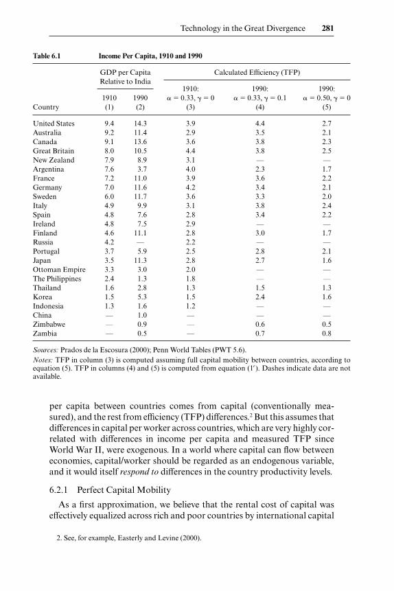
per capita between countries comes from capital (conventionally mea-sured), and the rest from efficiency (TFP) differences.2 But this assumes thatdifferences in capital per worker across countries, which are very highly cor-related with differences in income per capita and measured TFP sinceWorld War II, were exogenous. In a world where capital can flow betweeneconomies, capital/worker should be regarded as an endogenous variable,and it would itself respond to differences in the country productivity levels.

6.2.1 Perfect Capital Mobility

As a first approximation, we believe that the rental cost of capital waseffectively equalized across rich and poor countries by international capital


Table 6.1 Income Per Capita, 1910 and 1990

GDP per Capita Relative to India

Calculated Efficiency (TFP)

1910: 1990: 1990:1910 1990 � � 0.33, � � 0 � � 0.33, � � 0.1 � � 0.50, � � 0

Country (1) (2) (3) (4) (5)

United States 9.4 14.3 3.9 4.4 2.7Australia 9.2 11.4 2.9 3.5 2.1Canada 9.1 13.6 3.6 3.8 2.3Great Britain 8.0 10.5 4.4 3.8 2.5New Zealand 7.9 8.9 3.1 — —Argentina 7.6 3.7 4.0 2.3 1.7France 7.2 11.0 3.9 3.6 2.2Germany 7.0 11.6 4.2 3.4 2.1Sweden 6.0 11.7 3.6 3.3 2.0Italy 4.9 9.9 3.1 3.8 2.4Spain 4.8 7.6 2.8 3.4 2.2Ireland 4.8 7.5 2.9 — —Finland 4.6 11.1 2.8 3.0 1.7Russia 4.2 — 2.2 — —Portugal 3.7 5.9 2.5 2.8 2.1Japan 3.5 11.3 2.8 2.7 1.6Ottoman Empire 3.3 3.0 2.0 — —The Philippines 2.4 1.3 1.8 — —Thailand 1.6 2.8 1.3 1.5 1.3Korea 1.5 5.3 1.5 2.4 1.6Indonesia 1.3 1.6 1.2 — —China — 1.0 — — —Zimbabwe — 0.9 — 0.6 0.5Zambia — 0.5 — 0.7 0.8

Sources: Prados de la Escosura (2000); Penn World Tables (PWT 5.6).Notes: TFP in column (3) is computed assuming full capital mobility between countries, according toequation (5). TFP in columns (4) and (5) is computed from equation (1�). Dashes indicate data are notavailable.

2. See, for example, Easterly and Levine (2000).


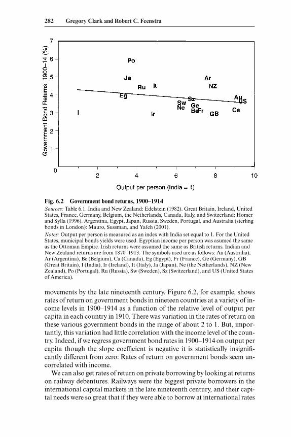
Fig. 6.2 Government bond returns, 1900–1914Sources: Table 6.1. India and New Zealand: Edelstein (1982). Great Britain, Ireland, UnitedStates, France, Germany, Belgium, the Netherlands, Canada, Italy, and Switzerland: Homerand Sylla (1996). Argentina, Egypt, Japan, Russia, Sweden, Portugal, and Australia (sterlingbonds in London): Mauro, Sussman, and Yafeh (2001).Notes: Output per person is measured as an index with India set equal to 1. For the UnitedStates, municipal bonds yields were used. Egyptian income per person was asumed the sameas the Ottoman Empire. Irish returns were assumed the same as British returns. Indian andNew Zealand returns are from 1870–1913. The symbols used are as follows: Au (Australia),Ar (Argentina), Be (Belgium), Ca (Canada), Eg (Egypt), Fr (France), Ge (Germany), GB(Great Britain), I (India), Ir (Ireland), It (Italy), Ja (Japan), Ne (the Netherlands), NZ (NewZealand), Po (Portugal), Ru (Russia), Sw (Sweden), Sz (Switzerland), and US (United Statesof America).

movements by the late nineteenth century. Figure 6.2, for example, showsrates of return on government bonds in nineteen countries at a variety of in-come levels in 1900–1914 as a function of the relative level of output percapita in each country in 1910. There was variation in the rates of return onthese various government bonds in the range of about 2 to 1. But, impor-tantly, this variation had little correlation with the income level of the coun-try. Indeed, if we regress government bond rates in 1900–1914 on output percapita though the slope coefficient is negative it is statistically insignifi-cantly different from zero: Rates of return on government bonds seem un-correlated with income.

We can also get rates of return on private borrowing by looking at returnson railway debentures. Railways were the biggest private borrowers in theinternational capital markets in the late nineteenth century, and their capi-tal needs were so great that if they were able to borrow at international rates

of return it would help equalize rates of return across all assets in domesticcapital markets. Table 6.2 shows the realized rates of return earned by in-vestors in railway debentures in the London capital market between 1870and 1913. Again, there are variations across countries. But, importantly forour purposes, this variation shows no correlation with output per person.Indeed, India, one of the poorest economies in the world, had among thelowest railway interest costs because the Indian government guaranteed thebonds of the railways as a way of promoting infrastructure investment. Thisrough equalization of returns to poor and rich countries was achieved bysignificant capital flows into these countries. By 1914 Egypt, the OttomanEmpire, Argentina, Brazil, Mexico, and Peru had all attracted at least £10per head of foreign investment (Pamuk 1987).

In a world of rapid capital mobility, how should we calculate TFP? Sup-pose as an approximation that the production function is Cobb-Douglas sothat

(1) Yi � AiKi�Li

�Ti� ,

where Ti denotes land and Ai the efficiency (TFP) of country i. Choose unitsso that Ai , Ki , Yi , and Ti are 1 in India. Taking capital stocks as exogenous,the income per capita of other economies relative to India would be

(2) �L

Yi

i

� � Ai��K

Li

i��

�

��L

Ti

i

��

.

The rental on capital can be computed by differentiating equation (1). Tak-ing this derivative and assuming the same rental on capital in all countries,then capital per worker in country i relative to India would be3


Table 6.2 Rates of Return on Railway Debentures, 1870–1913

Relative Output Per Capita Rate of ReturnCountry or Region (India � 1) (%)

United States 9.4 6.03Canada 9.1 4.99United Kingdom 7.9 3.74Argentina 7.6 5.13Brazil — 5.10

Western Europe 6.1 5.28Eastern Europe 4.1 5.33British India 1.0 3.65

Source: Table 1 in Edelstein (1982, 125).Note: Dash indicates data are not available.

3. The derivative of equation (1) with respect to Ki can be expressed as Ri � �Ai(Ki /Li )

(�–1)(Ti /Li )�. Dividing this entire expression by the same equation for India, which is as-

sumed to have the same rental Ri , we therefore obtain 1 � Ai (Ki /Li )(�–1)(Ti /Li)

�, where all vari-ables are now expressed relative to India. Then equation (3) follows directly.

(3) �K

Li

i� � Ai

1/(1��)��L

Ti

i

��(1��)

.

The amount of capital employed would thus depend on the level of effi-ciency of the economy. The more efficient an economy, the more capital itwould attract, which would have a second round effect in increasing incomeper person. Substituting equation (3) into equation (2), we obtain the fol-lowing expression for output per capita:

(4) �L

Yi

i

� � (Ai )1/(1��)��

L

Ti

i

��(1��)

.

Notice that the right-hand sides of equations (3) and (4) are identical, sothat capital/worker and output/worker are equal with capital endogenousand rates of return equalized across countries. It follows from equation (4)that we can calculate relative efficiencies in the world economy circa 1910as

(5) Ai � ��L

Yi

i

��1��L

Ti

i

��

.

Thus, in this case we can calculate relative TFP for each country relative toIndia from just the relative outputs per capita and the relative amount ofland per person. Since the share of land in national income, �, has becomevery small in recent years, equation (4) suggests that the sole significantcause of differences in income per capita between India and the UnitedStates and other advanced economies is differences in TFP.

6.2.2 Evidence from 1910

Even without reliable data on capital stocks across countries, we can cal-culate TFP from equation (5) if there is mobile capital. Column (3) of table6.1 and figure 6.3 show the implied TFP of the various countries in theworld in 1910 for which we have data, relative to India, assuming the shareof capital in national income was 0.33 and that of land was 0.1. Differencesin the land endowment per person were great enough that even assumingland had only a 10 percent share in output we seem to be overcorrecting forthe effect of land on income per capita. Thus there is no reason to believethat the efficiency of the U.S., Canadian, or Australian economies was re-ally below that of Great Britain in 1910. What we also see is that in a worldof free-flowing capital, modest differences in the efficiencies of economiesget translated into much bigger differences in income, through generationof additional savings by higher income and the movement of capital to thehigh-efficiency areas.

The assumption that capital invested was constant per unit of gross do-mestic product (GDP) might be regarded as unreasonable for 1910. Perhapsthen capital was not so mobile as now, so that poorer economies typically


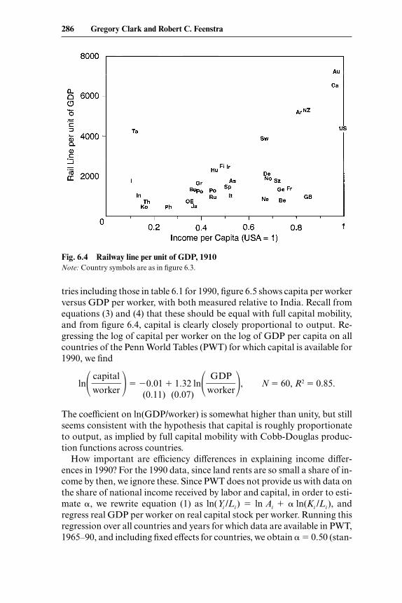
had smaller stocks of capital relative to output and higher returns on capi-tal. This proposition is difficult to test, but one partial measure is affordedby the amount of railway line per unit of GDP observed. Railways werehuge sinks of capital in the late nineteenth century and a popular vehicle forforeign investment. If capital was really scarce in the poor countries, thenalong with other investments the stock of rail line per unit of income shouldbe smaller the lower the income level per person. Figure 6.4 shows railwayline per unit of income as an index versus GDP per capita for a variety ofcountries in 1910. If we were to exclude the low-population-density settlercolonies of North America, Argentina, and Australasia, we would find thatpoor countries had as many miles of railway line per unit of GDP as richcountries.

6.2.3 Evidence from 1990

The assumption here that capital will be proportional to output findssupport in the international economy of the 1990s. Using a sample of coun-


Fig. 6.3 Calculated differences in efficiency (TFP) circa 1910Notes: Output per person is measured as an index with India set equal to 1. Efficiency ismeasured as an index with India again set to 1. The country symbols are as follows: A (Aus-tria), Au (Australia), Ar (Argentina), Be (Belgium), Bu (Burma), Ca (Canada), De (Den-mark), Fi (Finland), Fr (France), Ge (Germany), GB (Great Britain), Gr (Greece), Hu(Hungary), I (India), In (Indonesia), Ir (Ireland), It (Italy), Ja (Japan), Ko (Korea), Ne (theNetherlands), NZ (New Zealand), OE (Ottoman Empire), Ph (the Philippines), Po (Portu-gal), Ru (Russia), SL (Sri Lanka), Sp (Spain), Sw (Sweden), Sz (Switzerland), Th (Thailand),and US (United States).

tries including those in table 6.1 for 1990, figure 6.5 shows capita per workerversus GDP per worker, with both measured relative to India. Recall fromequations (3) and (4) that these should be equal with full capital mobility,and from figure 6.4, capital is clearly closely proportional to output. Re-gressing the log of capital per worker on the log of GDP per capita on allcountries of the Penn World Tables (PWT) for which capital is available for1990, we find

ln� � � �0.01 1.32 ln��wGoD

rk

P

er��, N � 60, R2 � 0.85.

(0.11) (0.07)

The coefficient on ln(GDP/worker) is somewhat higher than unity, but stillseems consistent with the hypothesis that capital is roughly proportionateto output, as implied by full capital mobility with Cobb-Douglas produc-tion functions across countries.

How important are efficiency differences in explaining income differ-ences in 1990? For the 1990 data, since land rents are so small a share of in-come by then, we ignore these. Since PWT does not provide us with data onthe share of national income received by labor and capital, in order to esti-mate �, we rewrite equation (1) as ln(Yi /Li ) � ln Ai � ln(Ki /Li ), andregress real GDP per worker on real capital stock per worker. Running thisregression over all countries and years for which data are available in PWT,1965–90, and including fixed effects for countries, we obtain � � 0.50 (stan-

capital�worker


Fig. 6.4 Railway line per unit of GDP, 1910Note: Country symbols are as in figure 6.3.


Fig. 6.5 Capital per worker versus GDP per worker, 1990Source: Penn World Tables (5.6).

dard error � 0.01). Performing the same regression in first differences,which still include fixed effects for countries, we obtain � � 0.34 (s.e. �0.04). Thus, the interval [0.33, 0.5] gives an adequate range for the share ofnational income going to capital, and this is quite consistent with our pri-ors for the capital share across various countries. In the final columns oftable 6.1 we report the calculation of TFP using these values of � and theformula

(1�) TFPi � Ai � �(

(

K

Y

i

i

/

/

L

L

i

i

)

)�

�,

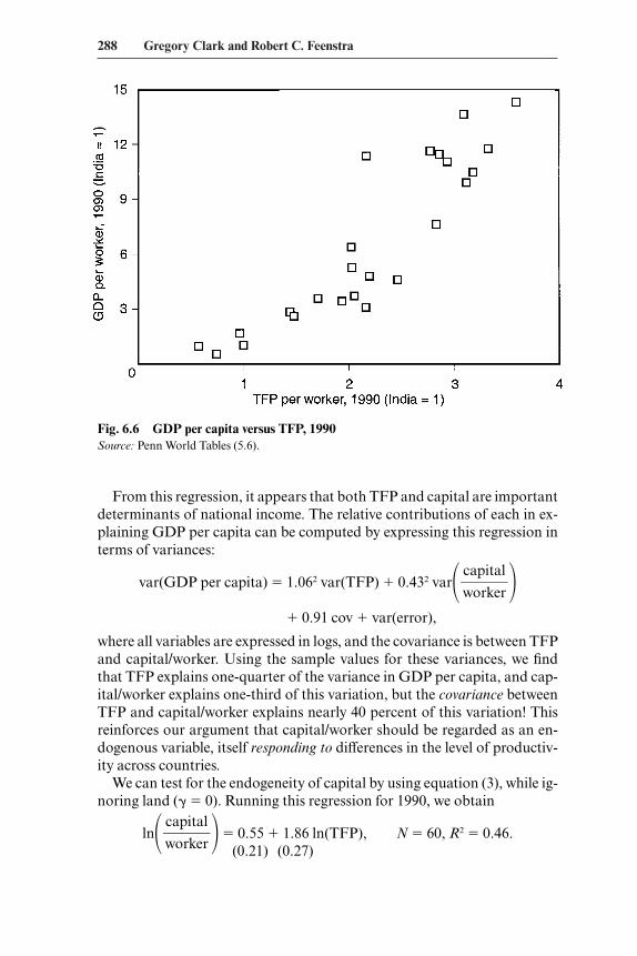
where all variables are measured relative to those in India.In figure 6.6, we graph real GDP per capita against TFP, using the inter-

mediate value of � � 0.4. There is quite clearly a strong positive relationshipbetween these measures of technology and income for the sample of coun-tries we have used. We saw above that capital per worker and GDP perworker are also closely linked. When GDP per capita is regressed againstboth these variables for 1990, we obtain

ln(GDP per capita) � �0.02 1.06 ln(TFP) 0.43 ln� � ,(0.04) (0.07) (0.03)

N � 60, R2 � 0.96.

capital�worker


Fig. 6.6 GDP per capita versus TFP, 1990Source: Penn World Tables (5.6).

From this regression, it appears that both TFP and capital are importantdeterminants of national income. The relative contributions of each in ex-plaining GDP per capita can be computed by expressing this regression interms of variances:

var(GDP per capita) � 1.062 var(TFP) 0.432 var� � 0.91 cov var(error),

where all variables are expressed in logs, and the covariance is between TFPand capital/worker. Using the sample values for these variances, we findthat TFP explains one-quarter of the variance in GDP per capita, and cap-ital/worker explains one-third of this variation, but the covariance betweenTFP and capital/worker explains nearly 40 percent of this variation! Thisreinforces our argument that capital/worker should be regarded as an en-dogenous variable, itself responding to differences in the level of productiv-ity across countries.

We can test for the endogeneity of capital by using equation (3), while ig-noring land (� � 0). Running this regression for 1990, we obtain

ln� � � 0.55 1.86 ln(TFP), N � 60, R2 � 0.46.(0.21) (0.27)

capital�worker

capital�worker


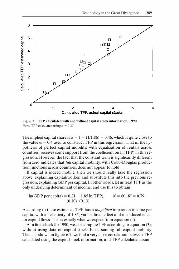
Fig. 6.7 TFP calculated with and without capital stock information, 1990Note: TFP calculated using � � 0.33.

The implied capital share is � � 1 � (1/1.86) � 0.46, which is quite close tothe value � � 0.4 used to construct TFP in this regression. That is, the hy-pothesis of perfect capital mobility, with equalization of rentals acrosscountries, receives some support from the coefficient on ln(TFP) in this re-gression. However, the fact that the constant term is significantly differentfrom zero indicates that full capital mobility, with Cobb-Douglas produc-tion functions across countries, does not appear to hold.

If capital is indeed mobile, then we should really take the regressionabove, explaining capital/worker, and substitute this into the previous re-gression, explaining GDP per capital. In other words, let us treat TFP as theonly underlying determinant of income, and use this to obtain

ln(GDP per capita) � 0.21 1.85 ln(TFP), N � 60, R2 � 0.79.(0.10) (0.13)

According to these estimates, TFP has a magnified impact on income percapita, with an elasticity of 1.85, via its direct effect and its induced effecton capital flows. This is exactly what we expect from equation (4).

As a final check for 1990, we can compute TFP according to equation (3),without using data on capital stocks but assuming full capital mobility.Then, as shown in figure 6.7, we find a very close correlation between TFPcalculated using the capital stock information, and TFP calculated assum-

ing that capital per worker is proportional to GDP per worker. The obser-vations mostly lie above the 45-degree line because India has a relativelysmall capital stock, and output per worker and capital per worker are bothmeasured relative to India. The correlation coefficient between the twomeasures is 0.96. Thus, by 1990 it seems plausible to regard TFP as the pri-mary driver of differences in income per capita across countries, with capi-tal playing a secondary and derivative role.

6.2.4 Imperfect Capital Mobility

Above we assumed perfect capital mobility. Since there likely were andare frictions in international capital markets, let us consider whether ourconclusion that income differences were driven by TFP differences has to beweakened once we allow for imperfect capital mobility, and therefore differ-ences in the rental on capital across countries. To see how differences in therental cost of capital modify our analysis, again compute the rental on cap-ital by differentiating equation (1). Allowing this to differ across countries,and expressing all variables in country i relative to India, we obtain4

(3�) �K

Li

i� � ��

A

Ri

i

��1/(1��)��L

Ti

i

��(1��)

.

Thus, the amount of capital employed will vary inversely with its rental,which now appears on the right of equation (3�). Substituting equation (3�)into equation (2), we obtain the following expression for output per capita:

(4�) �Y

Li

i� � (Ri )

��/(1��)(Ai )1/(1��)��

L

Ti

i

��/(1��)

.

Comparing equations (3�) and (4�), we see that capital/worker and out-put/worker differ by exactly the rental term, so that

(5�) �K

Li

i� � �

(Y

Ri /L

i

i )�.

Countries with lower rentals will attract more capital. Note that relativeTFP (with � � 0) can still be calculated as in equation (1�). The rental ofcapital is, of course, the product of the rate of return on capital in eachcountry and the purchase price of capital goods. The evidence we have onthe purchase price of capital goods for 1910 is the cost of fully equippedcotton spinning and weaving mills per spindle. This is a reasonably goodgeneral index of the cost of capital goods in these countries because cot-ton mills generally embodied imported machinery and power plants com-bined with local construction of the buildings. We also saw above little sign


4. From note 3, the rental on capital is Ri � �Ai (Ki /Li )(�–1)(Ti /Li)

�. Now divide this by thesame equation for India and express all variables relative to India, to obtain, Ri �Ai (Ki /Li)

(�–1)(Ti /Li )�. Then equation (3�) follows directly.

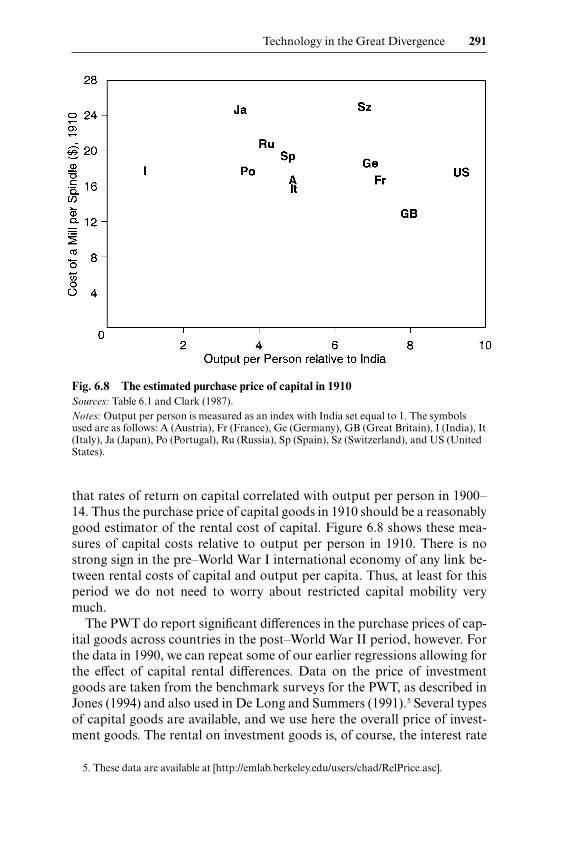
that rates of return on capital correlated with output per person in 1900–14. Thus the purchase price of capital goods in 1910 should be a reasonablygood estimator of the rental cost of capital. Figure 6.8 shows these mea-sures of capital costs relative to output per person in 1910. There is nostrong sign in the pre–World War I international economy of any link be-tween rental costs of capital and output per capita. Thus, at least for thisperiod we do not need to worry about restricted capital mobility verymuch.

The PWT do report significant differences in the purchase prices of cap-ital goods across countries in the post–World War II period, however. Forthe data in 1990, we can repeat some of our earlier regressions allowing forthe effect of capital rental differences. Data on the price of investmentgoods are taken from the benchmark surveys for the PWT, as described inJones (1994) and also used in De Long and Summers (1991).5 Several typesof capital goods are available, and we use here the overall price of invest-ment goods. The rental on investment goods is, of course, the interest rate


Fig. 6.8 The estimated purchase price of capital in 1910Sources: Table 6.1 and Clark (1987).Notes: Output per person is measured as an index with India set equal to 1. The symbolsused are as follows: A (Austria), Fr (France), Ge (Germany), GB (Great Britain), I (India), It(Italy), Ja (Japan), Po (Portugal), Ru (Russia), Sp (Spain), Sz (Switzerland), and US (UnitedStates).

5. These data are available at [http://emlab.berkeley.edu/users/chad/RelPrice.asc].

times its purchase price. For these years we do not have information on in-terest rates by country. However, provided that interest rates (and depreci-ation rates) do not vary with output per capita, we can use the purchaseprice of investment goods as a proxy for its rental in our estimations.

Regressing the log of capital per worker on the log of GDP per capita andalso the log of the rental, we obtain

ln� � � 0.17 1.16 ln� � � 0.47 ln(rental),

(0.11) (0.08) (0.23)

N � 52, R2 � 0.89.

The sample used here is on all countries of the PWT for which capital stocksare available for 1990, and we also have the price of investment goods in1980 reported in Jones (1994). The coefficient on ln(GDP/worker) is re-duced by inclusion of the rental, so that it becomes closer to unity. Therental itself has a negative coefficient, as predicted from (5�), but less thanunity; given the measurement error that is present in using the purchaseprice of investment goods rather than their rental, it is not surprising thatthis coefficient is biased toward zero.

Computing TFP according to equation (1�) using the value of � � 0.4, wecan treat this and the rental price of investment goods as the underlying de-terminants of income, and run equation (4�) to obtain

ln(GDP per capita) � 0.27 1.65 ln(TFP) � 0.67 ln(rental),

(0.08) (0.12) (0.18)

N � 52, R2 � 0.87.

Once again, we find that TFP has a magnified impact on income per capita,with an elasticity of 1.65, via its direct effect and its induced effect on capi-tal allocation. The relative contributions of TFP versus the rental in ex-plaining GDP per capita can be decomposed from this regression accord-ing to

var(GDP per capita) � 1.652 var(TFP) 0.672 var(rental)

� 2.21 cov var(error),

where the covariance is between TFP and the rental on investment goods.Using the sample values for these variances, we find that TFP explains fullytwo-thirds of the variance in GDP per capita, whereas the rental only ex-plains 5 percent of this variation, with the covariance between TFP and therental explaining another 16 percent of this variation. This, including therental on capital across countries, does not change our conclusion that TFPis the driving force behind differences in GDP per capita, with capital/worker responding to differences in the level of productivity.

GDP�worker

capital�worker


Where do these differences in productivity come from? Some recent au-thors have argued that geography or climate (Sachs 2001), or institutions(Acemoglu, Johnson, and Robinson 2001), or social capital (Jones and Hall1999) plays an important role. We do not dispute that these may be impor-tant, but our approach is different. Rather than looking for some externalcause for countries to differ in their efficiency levels, we will instead look in-ternally at productivity itself, and ask whether the cross-country variationin TFP should be attributed to the access to or to the use of technologies.

6.3 Access to Technology

We see that the increased disparity in income per capita across the worldstemmed largely from an increased disparity in the efficiency of economies,the amount of output produced per unit of input. The next thing we showis that little of this disparity stemmed from differences in access to technol-ogy. Economic growth since the Industrial Revolution has been largelybased on an expansion of knowledge. The fact that the Industrial Revolu-tion came from an increase in knowledge, rather than from capital accu-mulation or from the exploitation of natural resources, seemed to implythat it would spread with great rapidity to other parts of the world, for al-though developing new knowledge is an arduous task, copying innovationsis much easier. Also, although some of the new technology eventually wasvery sophisticated, some of it was relatively simple, or required little techni-cal expertise to operate. Thus, artificial fertilizers in the late nineteenth cen-tury, and new strains of crops in the twentieth, for example, which dramat-ically boosted agricultural yields, were both relatively simple technologiesfor poor countries to adopt. Further, given the possibilities of specializationin international trade, the poorer countries did not need to acquire all thenew Western technology. They could instead adopt the simplest and mosteasily transferable techniques, and import products embodying more so-phisticated processes from the more economically advanced countries. Intextiles, for example, spinning coarse yarn was much easier technically thanspinning fine yarn. Countries such as India could thus specialize in coarseyarn, and import finer cloth.

Further, there were a series of interrelated technical, organizational, andpolitical developments in the nineteenth century that made technologicaltransmission much easier. The important technological changes were theimprovements in transport through the development of railways, steam-ships, the Suez and (later) Panama canals, and the telegraph. The organiza-tional change was the development of specialized machine-building firms inGreat Britain and later the United States. The political changes were the ex-tension of European colonial empires to large parts of Africa and Asia, andthe political developments within European countries. By the eve of WorldWar I the first great globalization of the world economy was complete. Po-


litical and economic developments in the twentieth century disrupted thatearlier globalization, but even by 1914 it was clear that differences in theefficiency of economies could not be attributed just to differences in the typeof technology employed.

6.3.1 Transport and Communication

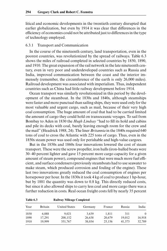
In the course of the nineteenth century, land transportation, even in thepoorest countries, was revolutionized by the spread of railways. Table 6.3shows the miles of railroad completed in selected countries by 1850, 1890,and 1910. The great expansion of the rail network in the late nineteenth cen-tury, even in very poor and underdeveloped countries such as Russia andIndia, improved communication between the coast and the interior im-mensely (remember, the circumference of the earth is only 26,000 miles).Railroad development was associated with imperialism. Thus, independentcountries such as China had little railway development before 1914.

Ocean transport was similarly revolutionized in this period by the devel-opment of the steamboat. In the 1830s and 1840s, although steamshipswere faster and more punctual than sailing ships, they were used only for themost valuable and urgent cargo, such as mail, because of their very highcoal consumption. The huge amount of coal that had to be carried limitedthe amount of cargo they could hold on transoceanic voyages. To sail fromBombay to Aden in 1830 the Hugh Lindsay “had to fill its hold and cabinsand pile its decks with coal, barely leaving enough room for the crew andthe mail” (Headrick 1988, 24). The liner Britannia in the 1840s required 640tons of coal to cross the Atlantic with 225 tons of cargo. Thus, even in the1850s steam power was used only for perishable and high-value cargoes.

But in the 1850s and 1860s four innovations lowered the cost of steamtransport. These were the screw propeller, iron hulls (iron-hulled boats were30–40 percent lighter and gave 15 percent more cargo capacity for a givenamount of steam power), compound engines that were much more fuel effi-cient, and surface condensers (previously steamboats had to use seawater tomake steam, which produced corrosion and fouling of the engine). Theselast two innovations greatly reduced the coal consumption of engines perhorsepower per hour. In the 1830s it took 4 kg of coal to produce 1 hp-hour,but by 1881 the quantity was down to 0.8 kg. This directly reduced costs,but since it also allowed ships to carry less coal and more cargo there was afurther reduction in costs. Real ocean freight costs fell by nearly 35 percent


Table 6.3 Railway Mileage Completed

Year Britain United States Germany France Russia India

1850 6,088 9,021 3,639 1,811 311 01890 17,291 208,152 26,638 20,679 19,012 16,9181910 19,999 351,767 38,034 25,156 41,373 32,789

from 1870 to 1910. In 1906, for example, it cost 8 shillings to carry a ton ofcotton goods by rail the thirty miles from Manchester to Liverpool, butonly 30 s. to ship those goods the 7,250 miles from Liverpool to Bombay.This cost of shipping cotton cloth was less than 1 percent of the cost of thegoods. By the late nineteenth century industrial locations with good wateraccess that were on well-established shipping routes—Bombay, Calcutta,Madras, Shanghai, Hong Kong—could get access to all the industrial in-puts of Great Britain at costs not very much higher than many British firms.In part this was because, since Great Britain’s exports were mainly manu-factures with high value per unit volume, there was excess shipping capac-ity on the leg out from Great Britain, making the transport of industrialmachinery and parts to underdeveloped countries such as India relativelycheap.

While freight costs fell, these technical advances also increased the speedof travel across the oceans. The fastest P&O (Peninsular and OrientalSteam Navigation Company) liner in 1842, the Hindustan, had a speed of10 knots per hour. By 1912 P&O’s fastest boat, the Maloja, could do 18knots. The speed of travel across oceans was further enhanced by the open-ing of the great canals, the Suez canal in 1869 and the Panama canal in 1914.The Suez canal alone saved 41 percent of the distance on the journey fromLondon to Bombay and 32 percent of the distance on the journey fromLondon to Shanghai. Thus, although in the 1840s it took sailing shipsfrom five to eight very uncomfortable months to get to India, by 1912 inprincipal the journey could be done in fifteen days.

The last of the important technical innovations in the late nineteenth cen-tury was the development of the telegraph. For the poorest countries ofAfrica and the East the key development was the invention of submarinecables for the telegraph. In the 1840s if an Indian firm bought British textilemachinery and ran into problems with it, it would take the firm at best tenmonths to receive any return communication from the machine builders. In1851 the first submarine telegraph cable was laid between France and En-gland. By 1865 India was linked to Great Britain by a telegraph systempartly over land that could transmit messages in twenty-four hours, and in1866 a successful transatlantic telegraph service had been established.Thus, by 1866 orders and instructions could be communicated halfwayacross the world in days.

These changes together made the world a much smaller place in the latenineteenth century than it had been earlier. Information could travel muchfaster. We know, for example, that the average time it took news to travelfrom Rome to Cairo in the first three centuries .., when Egypt was aprovince of the Roman Empire, was about one mile per hour. As late as theearly eighteenth century it had taken four days to send letters 200 mileswithin Great Britain. With the telegraph, rail, and steamship it was possibleto send information across the world in much less time. The steamship and


railroad also made travel faster and much more reliable for people andgoods. And the development of the steamship made the cost of reachingfar-flung places quite low as long as they had good access to ocean naviga-tion. The technological basis for the export of Industrial Revolution tech-nologies to almost any country in the world thus seemed to have been com-pleted by the last quarter of the nineteenth century.

6.3.2 Organizational Changes

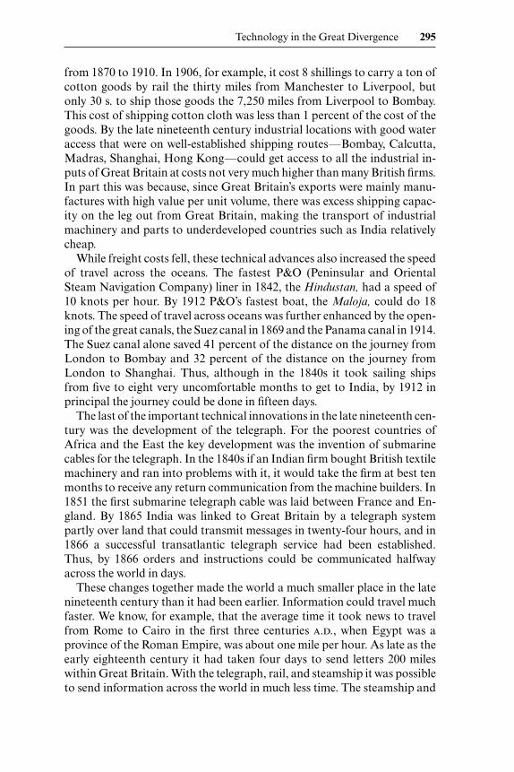
In the early nineteenth century a specialized machine-building sector de-veloped within the Lancashire cotton industry. These machinery firms,some of which (such as Platt) were exporting at least 50 percent of their pro-duction as early as 1845–70, had an important role in exporting textile tech-nology. These capital goods firms were able to provide a complete packageof services to prospective foreign entrants to the textile industry, which in-cluded technical information, machinery, construction expertise, and man-agers and skilled operatives. By 1913 the six largest machine producers em-ployed over 30,000 workers (Bruland 1989, 5, 6, 34). These firms reducedthe risks to foreign entrepreneurs by such practices as giving them machineson a trial basis and undertaking to supply skilled workers to train the locallabor force. As a result, firms like Platt sold all around the world. Table 6.4shows the number of orders for ring-spinning frames Platt took (each ordertypically involved numbers of machines) for a sample of nine years in eachof the periods 1890–1914 and 1915–1934. Indeed, for ring frames Englandwas a small share of Platt’s market throughout these years.

Similar capital goods exporters developed in the rail sectors, and later inthe United States in the boot and shoe industry. British construction crewscompleted railways in many foreign countries under the captainship of suchflamboyant entrepreneurs as Lord Brassey. The reason again for the over-seas exodus was in part the saturation of the rail market within GreatBritain by the 1870s after the boom years of railway construction. By 1875,in a boom lasting just forty-five years, 71 percent of all the railway line everconstructed in Great Britain was completed. Thereafter the major marketsfor British contractors and engine constructors were overseas. India, for ex-ample, got most of its railway equipment from Great Britain, and the In-dian railway mileage by 1910 was significantly greater than the British, astable 6.3 has shown.

6.3.3 Political Developments

A number of political developments should have speeded up the exportof technology in the nineteenth century. The most important of these wasthe expansion of the European colonial territories. By 1900 the Europeanpowers controlled as colonies 35 percent of the land surface of the world,even excluding from this reckoning Asiatic Russia. Thus, of a world area of57.7 million square miles Europe itself constitutes only 3.8 million square


miles, but by 1900 its dependencies covered 19.8 million square miles. TheBritish Empire was the largest, covering 9.0 million square miles; theFrench had 4.6 million, the Netherlands 2.0 million, and Germany 1.2 mil-lion.

Even many countries formally outside of the control of European pow-ers were forced to cede trading privileges and special rights to Europeans.Thus, China was forced in the course of the nineteenth century to cede var-ious treaty ports, such as Shanghai. The political control by countries suchas Great Britain of so much of the world allowed entrepreneurs to exportmachinery and techniques to low-wage areas with little risk of expropria-tion. Thus the great increase in the scope and effectiveness of British polit-ical power in the course of the nineteenth century made it easier to exportcapital from Great Britain to support new textile industries. Most of the In-


Table 6.4 Platt Ring Frame Orders by Country, 1890–1934

Sales, 1890–1914 Sales, 1914–36Country (9 years) (9 years)

Austria 4 0Belgium 17 15Brazil 95 43Canada 15 17China 5 64Czechoslovakia 14 10Egypt 0 5England 110 74Finland 1 0France 41 31Germany 47 6Guatemala 1 1Hungary 0 4India 66 132Italy 69 29Japan 66 117Mexico 75 7The Netherlands 7 2Nicaragua 2 0Peru 7 0Poland 41 8Portugal 8 0Russia 131 23Spain 95 35Sweden 3 0Switzerland 3 0Turkey 0 6United States 2 0West Africa 0 2

Source: Lancashire Record Office.

dian subcontinent and Burma was brought under British administrativecontrol in 1858, and Egypt fell to Britain in 1882. In 1842 the British securedHong Kong from China, and in 1858 they achieved a concession in Shang-hai. These were all localities with very low wage rates and easy access to ma-jor sea routes. The joint effect of these technological and political develop-ments was to create by 1900 an expanded British economy spanning theglobe. British policy within its empire was to eliminate barriers to trade andto allow economic activity to proceed wherever the market deemed mostprofitable. In India, for example, despite protests from local interests theBritish insisted on a free trade policy between Great Britain and India. Anymanufacturer who set up a cotton mill in Bombay was assured of access tothe British market on the same terms as British mills.

The nature of British imperialism also ensured that no country was re-strained from the development of industry up until 1917 by the absence ofa local market of sufficient size. Because of the British policy of free tradepursued in the nineteenth century, Great Britain itself and most British de-pendencies were open to imports with no tariff or else a low tariff for rev-enue purposes only. The large Indian market, which took a large share ofEnglish textile production, for example, was open on the same terms to allforeign producers. There was a 3.5 percent revenue tariff on imports, but acountervailing tax was applied to local Indian mills at the insistence ofManchester manufacturers. The Chinese textile market, at the insistence ofthe imperial powers, was also protected by a 5 percent ad valorem revenuetariff.

6.4 Efficiency in the Use of Technology

Although railways, cotton mills, and other advanced technologies spreadrapidly around the world by the late nineteenth century as a result of theabove factors, the efficiency with which this technology was used differedgreatly across countries. It was this inefficiency in use that in practice lim-ited the spread of new production technologies. We illustrate this using theexample of the railroads, but an equivalent story can be told for cotton tex-tiles (Clark 1987; Wolcott and Clark 1999).

Output in each country is measured as a weighted sum of the number oftons of freight hauled, the ton-miles of freight, and passenger-miles of pas-sengers. Both tons of freight and ton-miles were used because the averagelength of haul varied greatly and the fixed costs in hauling freight from load-ing and unloading were substantial compared to the costs of hauling goodsanother ton-mile.6 Freight output was thus estimated as (tons $0.285 ton-miles $0.0066). The quality of passenger service varied greatly, which


6. From freight revenues across countries we estimate that the cost of freight hauling a tonof freight x miles in the United States in 1914 in $(0.285 0.0066z).

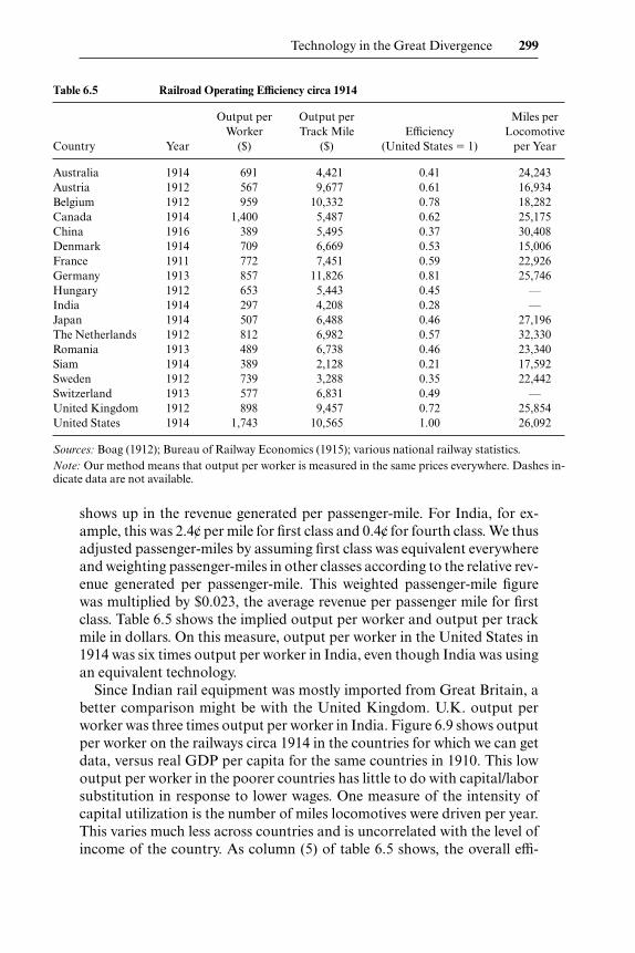
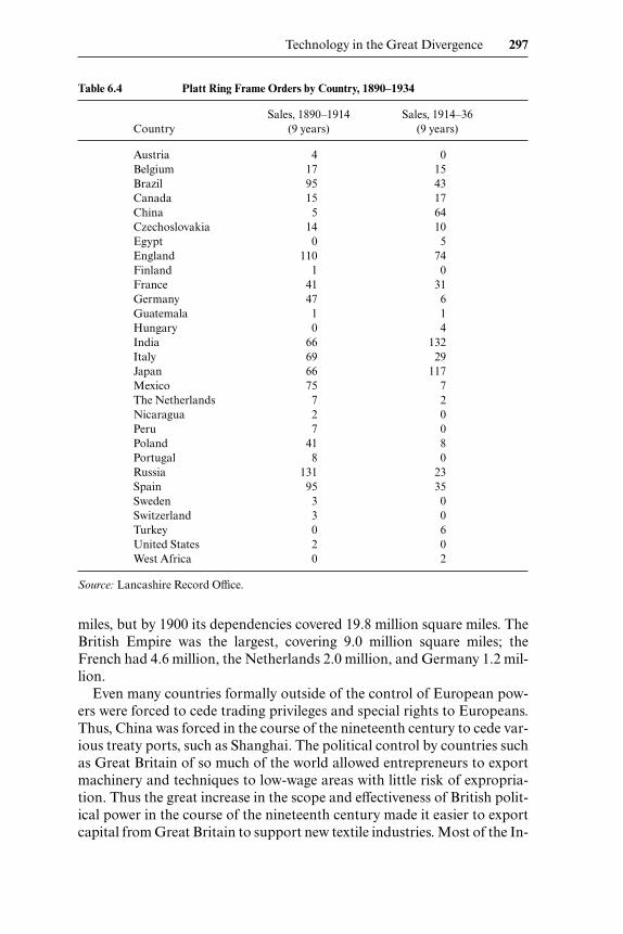
shows up in the revenue generated per passenger-mile. For India, for ex-ample, this was 2.4¢ per mile for first class and 0.4¢ for fourth class. We thusadjusted passenger-miles by assuming first class was equivalent everywhereand weighting passenger-miles in other classes according to the relative rev-enue generated per passenger-mile. This weighted passenger-mile figurewas multiplied by $0.023, the average revenue per passenger mile for firstclass. Table 6.5 shows the implied output per worker and output per trackmile in dollars. On this measure, output per worker in the United States in1914 was six times output per worker in India, even though India was usingan equivalent technology.

Since Indian rail equipment was mostly imported from Great Britain, abetter comparison might be with the United Kingdom. U.K. output perworker was three times output per worker in India. Figure 6.9 shows outputper worker on the railways circa 1914 in the countries for which we can getdata, versus real GDP per capita for the same countries in 1910. This lowoutput per worker in the poorer countries has little to do with capital/laborsubstitution in response to lower wages. One measure of the intensity ofcapital utilization is the number of miles locomotives were driven per year.This varies much less across countries and is uncorrelated with the level ofincome of the country. As column (5) of table 6.5 shows, the overall effi-


Table 6.5 Railroad Operating Efficiency circa 1914

Output per Output per Miles perWorker Track Mile Efficiency Locomotive

Country Year ($) ($) (United States � 1) per Year

Australia 1914 691 4,421 0.41 24,243Austria 1912 567 9,677 0.61 16,934Belgium 1912 959 10,332 0.78 18,282Canada 1914 1,400 5,487 0.62 25,175China 1916 389 5,495 0.37 30,408Denmark 1914 709 6,669 0.53 15,006France 1911 772 7,451 0.59 22,926Germany 1913 857 11,826 0.81 25,746Hungary 1912 653 5,443 0.45 —India 1914 297 4,208 0.28 —Japan 1914 507 6,488 0.46 27,196The Netherlands 1912 812 6,982 0.57 32,330Romania 1913 489 6,738 0.46 23,340Siam 1914 389 2,128 0.21 17,592Sweden 1912 739 3,288 0.35 22,442Switzerland 1913 577 6,831 0.49 —United Kingdom 1912 898 9,457 0.72 25,854United States 1914 1,743 10,565 1.00 26,092

Sources: Boag (1912); Bureau of Railway Economics (1915); various national railway statistics.Note: Our method means that output per worker is measured in the same prices everywhere. Dashes in-dicate data are not available.

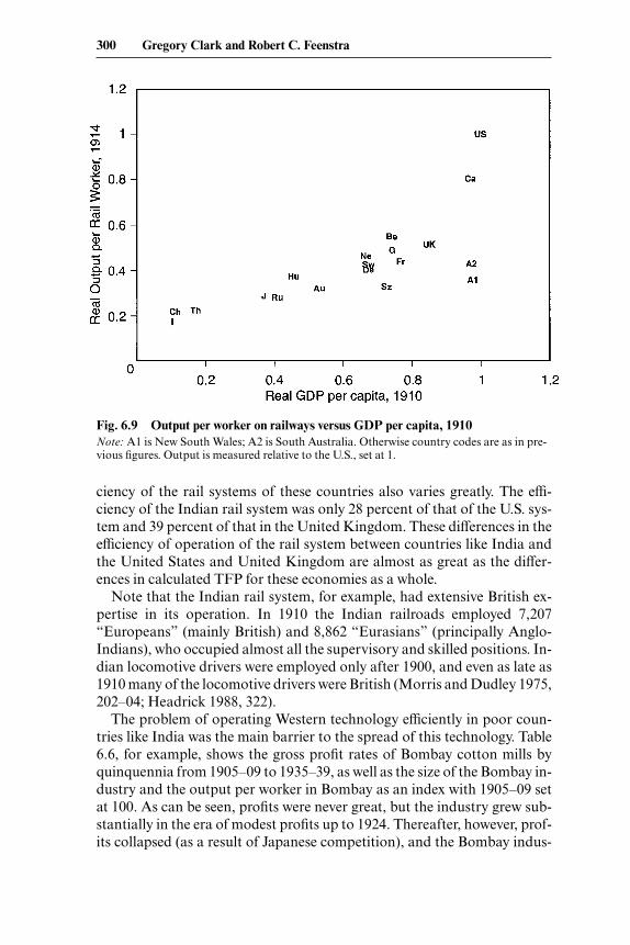
ciency of the rail systems of these countries also varies greatly. The effi-ciency of the Indian rail system was only 28 percent of that of the U.S. sys-tem and 39 percent of that in the United Kingdom. These differences in theefficiency of operation of the rail system between countries like India andthe United States and United Kingdom are almost as great as the differ-ences in calculated TFP for these economies as a whole.

Note that the Indian rail system, for example, had extensive British ex-pertise in its operation. In 1910 the Indian railroads employed 7,207“Europeans” (mainly British) and 8,862 “Eurasians” (principally Anglo-Indians), who occupied almost all the supervisory and skilled positions. In-dian locomotive drivers were employed only after 1900, and even as late as1910 many of the locomotive drivers were British (Morris and Dudley 1975,202–04; Headrick 1988, 322).

The problem of operating Western technology efficiently in poor coun-tries like India was the main barrier to the spread of this technology. Table6.6, for example, shows the gross profit rates of Bombay cotton mills byquinquennia from 1905–09 to 1935–39, as well as the size of the Bombay in-dustry and the output per worker in Bombay as an index with 1905–09 setat 100. As can be seen, profits were never great, but the industry grew sub-stantially in the era of modest profits up to 1924. Thereafter, however, prof-its collapsed (as a result of Japanese competition), and the Bombay indus-


Fig. 6.9 Output per worker on railways versus GDP per capita, 1910Note: A1 is New South Wales; A2 is South Australia. Otherwise country codes are as in pre-vious figures. Output is measured relative to the U.S., set at 1.

try soon began to contract. The last column shows what was happening tooutput per worker in Japan, where, with the same machinery as in India (inboth cases purchased from England), output per worker increased greatly.

Thus, the crucial variable in explaining the success or failure of economiesin the years 1800–2000 seems to be the efficiency of the production processwithin the economy. And the differences in the ability to employ technologyseemingly got larger over time between rich and poor countries.

6.5 Trade Patterns and the Sources of Inefficiency

Despite the importance of TFP differences, we have very little idea whatgenerates them. We now consider using the pattern of trade to determinewhether these TFP differences specifically adhered to labor in poor coun-tries, or lay in some wider managerial failure.

The dominance of Great Britain and its free trade ideology in much of theworld circa 1910 meant that trade barriers were low for the countries withthe majority of world population in 1910—India (including modern Pak-istan, Bangladesh, and Burma), China, Great Britain, Ireland, Egypt,Nigeria, and South Africa. However, the trade patterns for the factors ofproduction within this relatively open world market were often not what wemight expect. In particular, the densely populated countries of the East—India, China, and Egypt (counting the cultivable land)—seem to have beennet exporters of land and net importers of labor. Table 6.7, for example,shows British India’s commodity trade in 1912. The only manufacturedgood that India exported any quantity of was jute sacking. In the case ofcotton the raw material content of India’s exports of raw cotton aboutequaled in value the raw material value of India’s imports. Thus India effec-tively exported its raw cotton to Great Britain to be manufactured there,paying for this with the export of other raw materials. The effective net raw


Table 6.6 The Bombay Industry, 1907–38

Gross Profit Size of the Bombay Output per Output perRate on Fixed Industry (millions of Worker in Bombay Worker in Japan

Year Capital spindle-equivalents) (index) (index)

1905–09 0.06 3.09 100 1001910–14 0.05 3.43 103 1151915–19 0.07 3.68 99 1351920–24 0.08 4.05 94 1321925–29 –0.00 4.49 91 1801930–34 0.00 4.40 104 2491935–39 0.02 3.91 106 281

Source: Wolcott and Clark (1999).Note: Profits and output per worker were calculable only for the mills listed in the Investor’s India Year-book (various years).

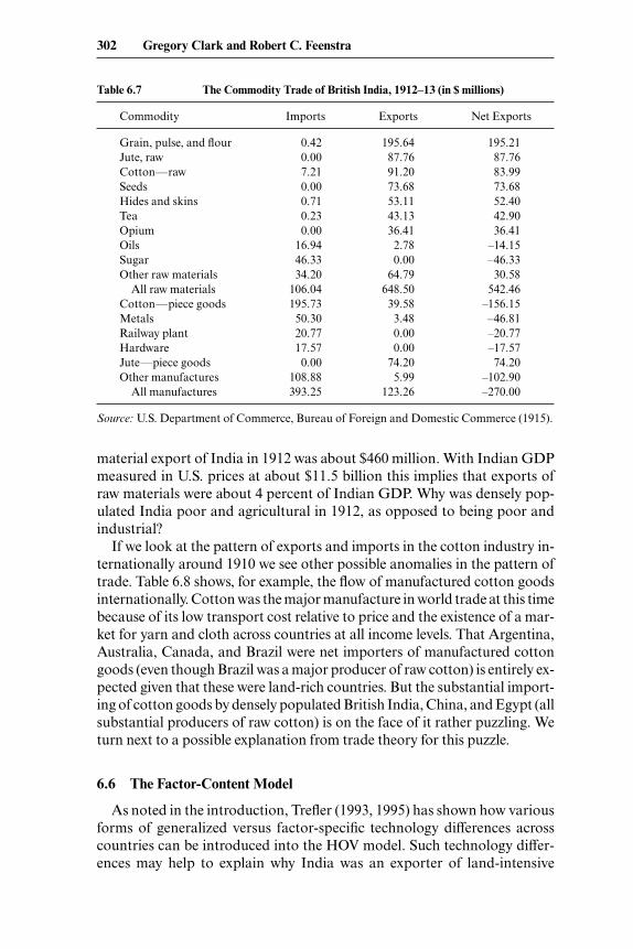
material export of India in 1912 was about $460 million. With Indian GDPmeasured in U.S. prices at about $11.5 billion this implies that exports ofraw materials were about 4 percent of Indian GDP. Why was densely pop-ulated India poor and agricultural in 1912, as opposed to being poor andindustrial?

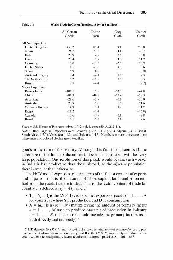
If we look at the pattern of exports and imports in the cotton industry in-ternationally around 1910 we see other possible anomalies in the pattern oftrade. Table 6.8 shows, for example, the flow of manufactured cotton goodsinternationally. Cotton was the major manufacture in world trade at this timebecause of its low transport cost relative to price and the existence of a mar-ket for yarn and cloth across countries at all income levels. That Argentina,Australia, Canada, and Brazil were net importers of manufactured cottongoods (even though Brazil was a major producer of raw cotton) is entirely ex-pected given that these were land-rich countries. But the substantial import-ing of cotton goods by densely populated British India, China, and Egypt (allsubstantial producers of raw cotton) is on the face of it rather puzzling. Weturn next to a possible explanation from trade theory for this puzzle.

6.6 The Factor-Content Model

As noted in the introduction, Trefler (1993, 1995) has shown how variousforms of generalized versus factor-specific technology differences acrosscountries can be introduced into the HOV model. Such technology differ-ences may help to explain why India was an exporter of land-intensive


Table 6.7 The Commodity Trade of British India, 1912–13 (in $ millions)

Commodity Imports Exports Net Exports

Grain, pulse, and flour 0.42 195.64 195.21Jute, raw 0.00 87.76 87.76Cotton—raw 7.21 91.20 83.99Seeds 0.00 73.68 73.68Hides and skins 0.71 53.11 52.40Tea 0.23 43.13 42.90Opium 0.00 36.41 36.41Oils 16.94 2.78 –14.15Sugar 46.33 0.00 –46.33Other raw materials 34.20 64.79 30.58

All raw materials 106.04 648.50 542.46Cotton—piece goods 195.73 39.58 –156.15Metals 50.30 3.48 –46.81Railway plant 20.77 0.00 –20.77Hardware 17.57 0.00 –17.57Jute—piece goods 0.00 74.20 74.20Other manufactures 108.88 5.99 –102.90

All manufactures 393.25 123.26 –270.00

Source: U.S. Department of Commerce, Bureau of Foreign and Domestic Commerce (1915).

goods at the turn of the century. Although this fact is consistent with thesheer size of the Indian subcontinent, it seems inconsistent with her verylarge population. One resolution of this puzzle would be that each workerin India is less productive than those abroad, so the effective populationthere is smaller than otherwise.

The HOV model expresses trade in terms of the factor content of exportsand imports—that is, the amounts of labor, capital, land, and so on em-bodied in the goods that are traded. That is, the factor content of trade forcountry c is defined as Fc � ATc , where

• Tc � Yc – Dc is the (N 1) vector of net exports of goods i � 1, . . . , Nfor country c, where Yc is production and Dc is consumption;

• A � [aki ] is a (M N ) matrix giving the amount of primary factor k � 1, . . . , M used to produce one unit of production in industry i � 1, . . . , N. (This matrix should include the primary factors usedboth directly and indirectly).7


Table 6.8 World Trade in Cotton Textiles, 1910 (in $ millions)

All Cotton Cotton Grey ColoredGoods Yarn Cloth Cloth

All Net ExportersUnited Kingdom 453.2 83.4 99.8 270.0Japan 26.2 22.3 4.6 –0.7Italy 23.9 4.2 2.9 16.8France 23.4 –2.7 4.3 21.9Germany 15.0 –11.3 –2.7 28.9United States 8.5 –3.5 8.3 3.6Spain 5.9 0.0 (5.9)Austria-Hungary 3.4 –4.1 0.2 7.3The Netherlands 3.2 –13.8 7.5 9.5Russia 2.7 –4.4 (7.2)

Major ImportersBritish India –100.1 17.8 –53.1 –64.8China –80.9 –40.8 –10.6 –29.5Argentina –28.6 –2.7 –0.9 –25.0Australia –24.8 –2.0 –1.2 –21.6Ottoman Empire –19.7 –1.1 –7.4 –11.2Egypt –18.2 –1.4 (–16.8)Canada –11.6 –1.9 –0.8 –8.8Brazil –11.1 –2.5 0.0 –8.6

Source: U.S. House of Representatives (1912, vol. 1, appendix A, 212–18).Notes: Other large net importers were Romania (–9.9), Chile (–9.3), Algeria (–9.2), BritishSouth Africa (–7.7), Venezuela (–4.3), and Bulgaria (–4.3). Numbers in parentheses are thosewhere gray and colored cloth is given together.

7. If D denotes the (K N ) matrix giving the direct requirements of primary factors to pro-duce one unit of output in each industry, and B is the (N N ) input-output matrix for thecountry, then the total primary factor requirements are computed as A � D(I – B)–1.

Focusing on the case in which labor, capital, and land are the primary fac-tors, then Fc � (FLc , FKc , FTc ) will have three elements, giving the net exportsof these factors for country c. Notice that we have not included a subscripton the matrix A, and because it is difficult to obtain the primary factors re-quirement for many countries, the convention has been to use A for a basecountry—say, the United Kingdom. At the same time, we allow for a gen-eral pattern of factor-specific productivity differences across countries, sothat factor k used in country c has productivity �kc , where these are mea-sured relative to the productivity in the base country.

Consistent with the measurement of Fc using the technology of the basecountry, Trefler (1995) extends the HOV model to show how the factor-content of trade is related to the effective endowments labor, capital, andland, where these are measured in efficiency units �kc . That is, letting �LcLc ,�KcKc , �TcTc denote the effective endowments of the factors in country c, theHOV model predicts that

(6A) FLc � �LcLc � sc ∑C

j�0

�LjLj

(6B) FKc � �KcKc � sc ∑C

j�0

�KjKj

(6C) FTc � �TcTc � sc ∑C

j�0

�TjTj

where sc � Yc /∑Cj�0Yj denotes the share of country c’s GDP in world GDP.8

To interpret these equations, equation (6A) states that country c will be anet exporter of labor services, FLc � 0, if its effective endowment of labor,�LcLc, exceeds its GDP share sc times the world effective endowment of la-bor, ∑C

j�0�LjLj . Put simply, if country c is abundant in labor (with �LcLc /∑C

j�0�LjLj � sc ), then it will be a net exporter of labor. A similar interpreta-tion holds for the other factors.

Let us now return to the puzzle: Why was India a net exporter of land-intensive products around the turn of the century? We interpret this state-ment to mean that if the full factor content calculation were done, Indiawould be found to be a net exporter of land, so that FTc � 0. In addition, weexpect that India would be found to be a net importer of either capital, FKc 0, or labor, FLc 0. Thus, for India we would write equations (6A)–(6C) as

(7A) �LcLc � sc ∑C

j�0

�LjLj 0, or

(7B) �KcKc � sc ∑C

j�0

�KjKj 0, and


8. More precisely, sc denotes the share of country c’s consumption in world consumption, butthis will equal its share of world GDP if trade is balanced for country c.

(7C) �TcTc � sc ∑C

j�0

�TjTj � 0.

Depending on whether inequality (7A) or (7B) holds, these taken togetherwith (7C) imply that

(8) �∑C

�

j�

L

0

c

�

L

L

c

jLj

� sc �∑�Cj�

T

0

c

�

Tc

TjTj

� , or �∑�Cj�

K

0

c

�

K

K

c

jKj

� sc �∑�Cj�

T

0

c

�

T

T

c

jTj

�.

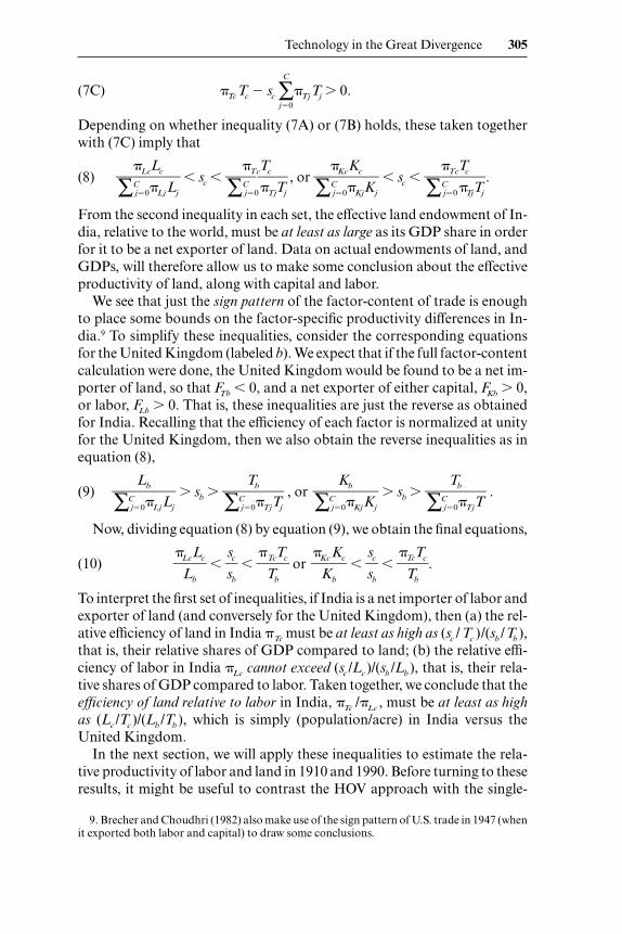
From the second inequality in each set, the effective land endowment of In-dia, relative to the world, must be at least as large as its GDP share in orderfor it to be a net exporter of land. Data on actual endowments of land, andGDPs, will therefore allow us to make some conclusion about the effectiveproductivity of land, along with capital and labor.

We see that just the sign pattern of the factor-content of trade is enoughto place some bounds on the factor-specific productivity differences in In-dia.9 To simplify these inequalities, consider the corresponding equationsfor the United Kingdom (labeled b). We expect that if the full factor-contentcalculation were done, the United Kingdom would be found to be a net im-porter of land, so that FTb 0, and a net exporter of either capital, FKb � 0,or labor, FLb � 0. That is, these inequalities are just the reverse as obtainedfor India. Recalling that the efficiency of each factor is normalized at unityfor the United Kingdom, then we also obtain the reverse inequalities as inequation (8),

(9) �∑Cj�

L

0�

b

LjLj

� � sb � �∑Cj�

T

0

b

�TjTj

� , or �∑Cj�

K

0�

b

KjKj

� � sb � �∑Cj�

T

0

b

�TjT� .

Now, dividing equation (8) by equation (9), we obtain the final equations,

(10) ��L

Lc

b

Lc� �

s

sc

b

� ��

TTc

b

Tc� or �

�K

KcK

b

c� �

s

sc

b

� ��

TTc

b

Tc�.

To interpret the first set of inequalities, if India is a net importer of labor andexporter of land (and conversely for the United Kingdom), then (a) the rel-ative efficiency of land in India �Tc must be at least as high as (sc / Tc )/(sb /Tb ),that is, their relative shares of GDP compared to land; (b) the relative effi-ciency of labor in India �Lc cannot exceed (sc /Lc )/(sb /Lb ), that is, their rela-tive shares of GDP compared to labor. Taken together, we conclude that theefficiency of land relative to labor in India, �Tc /�Lc , must be at least as highas (Lc /Tc )/(Lb /Tb ), which is simply (population/acre) in India versus theUnited Kingdom.

In the next section, we will apply these inequalities to estimate the rela-tive productivity of labor and land in 1910 and 1990. Before turning to theseresults, it might be useful to contrast the HOV approach with the single-


9. Brecher and Choudhri (1982) also make use of the sign pattern of U.S. trade in 1947 (whenit exported both labor and capital) to draw some conclusions.

sector Cobb-Douglas function used earlier in the paper. With the single sec-tor, we were assuming that TFP varied across countries and acted as a driv-ing force behind capital mobility. We ignored the contribution of land tototal GDP in modern times. Once we introduce trade data, however, itbecomes quite relevant to incorporate trade in agricultural goods, and theamount of land embodied in trade. In our calculations below, we will focuson the labor and land content of trade, while ignoring capital embodied intrade. Thus, we do not need to take any stand on the extent of capital flowsbetween countries, and how this responds to productivity. Rather, we willsimply treat the labor and land endowments as exogenous across countries,although differing in their productivities, and use their endowments com-bined with the factor contents of trade to infer the factor productivities.

6.7 Evidence from the Sign Pattern of Trade

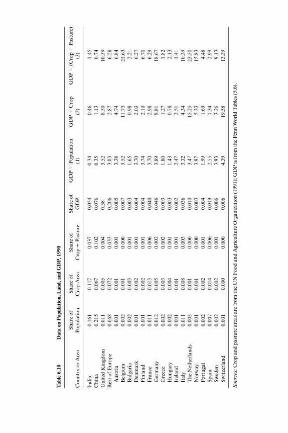
To illustrate these calculations, some data on population, land area,GDP, and their ratios are shown in table 6.9 for 1910 and in table 6.10 for1990. These are all measured relative to world totals. For example, the fig-ure of 0.36 for GDP/population in India for 1910 indicates that India has 36percent of the world average GDP per capita. Surprisingly, this number re-mained much the same in 1990 (dropping just slightly to 0.34), although thisfinding relies on the fact that we are using the purchasing power parity(PPP)–adjusted GDP values from the PWT. Prices are so low in India thatits GDP is 3.5 times higher in the PWT for 1990 than obtained from WorldBank data, which convert its nominal GDP to dollars with current ex-change rates. In contrast to the roughly constant value for India, most Eu-ropean nations have increased their level of real GDP per capita relative tothe world, in some cases nearly doubling their world share. This is consis-tent with the divergence in income levels described in section 6.2, of course.We also report GDP relative to crop acreage, or crop plus pasture, and theseshow a mixed pattern between 1910 and 1990—increasing for some Euro-pean nations relative to the world, but falling for others.

To use these data to estimate the productivity of factors, we focus on In-dia relative to some comparison countries. Choosing the United Kingdomas the initial comparison, we use the first set of inequalities in equation (10).Then their ratio of per capita GDP is shown in the column marked (1) intable 6.11, which provides an upper bound to the efficiency of labor in Indiarelative to the United Kingdom. The value of 0.13 indicates that an Indianworker is less than 13 percent as productive as his counterpart in the UnitedKingdom.10 The ratios of GDP to crop land or crop plus pasture are shownin columns (2) and (3), and provide lower bounds to the efficiency of land in


10. Rather than using total population in tables 6.9 and 6.10, we should actually use esti-mates of the workforce.

Tab

le 6

.9D

ata

on P

opul

atio

n, L

and,

and

GD

P, c

irca

191

0

Shar

e of

Shar

e of

Shar

e of

Shar

e of

GD

P �

Popu

lati

onG

DP

�C

rop

GD

P �

(Cro

p

Pas

ture

)C

ount

ry o

r A

rea

Popu

lati

onC

rop

Are

aC

rop

P

astu

reG

DP

(1)

(2)

(3)

Indi

a0.

169

0.11

40.

044

0.06

10.

360.

541.

40C

hina

0.31

20.

079

0.07

40.

116

0.37

1.47

1.57

Uni

ted

Kin

gdom

0.02

30.

005

0.00

50.

064

2.82

12.5

712

.86

Res

t of E

urop

e0.

197

0.10

40.

054

0.36

01.

833.

456.

67A

ustr

ia0.

004

0.00

10.

001

0.00

71.

775.

136.

22B

elgi

um0.

004

0.00

10.

000

0.01

02.

4714

.31

23.0

4B

ulga

ria

0.00

20.

003

0.00

10.

003

1.23

0.96

2.53

Den

mar

k0.

002

0.00

20.

001

0.00

32.

251.

734.

27F

inla

nd0.

002

0.00

20.

001

0.00

31.

631.

433.

59F

ranc

e0.

022

0.01

50.

009

0.05

62.

563.

636.

26G

erm

any

0.03

60.

010

0.00

50.

089

2.46

8.91

16.5

6G

reec

e0.

001

0.00

30.

002

0.00

21.

300.

750.

85H

unga

ry0.

004

0.00

40.

002

0.00

61.

531.

573.

50Ir

elan

d0.

002

0.00

10.

001

0.00

41.

714.

093.

41It

aly

0.01

90.

011

0.00

50.

034

1.75

2.97

6.26

The

Net

herl

ands

0.00

30.

001

0.00

10.

007

2.22

9.54

12.1

8N

orw

ay0.

001

0.00

10.

000

0.00

32.

275.

0211

.36

Port

ugal

0.00

30.

003

0.00

10.

004

1.31

1.47

4.10

Spai

n0.

011

0.01

50.

006

0.01

91.

701.

273.

34Sw

eden

0.00

30.

003

0.00

10.

007

2.23

2.60

6.13

Swit

zerl

and

0.00

20.

000

0.00

10.

005

2.41

15.7

29.

00

Sou

rce:

Cro

p an

d pa

stur

e ar

eas

are

from

the

UN

Foo

d an

d A

gric

ultu

re O

rgan

izat

ion

(199

1) a

nd a

pply

to y

ears

aro

und

1957

.

Tab

le 6

.10

Dat

a on

Pop

ulat

ion,

Lan

d, a

nd G

DP,

199

0

Shar

e of

Shar

e of

Shar

e of

Shar

e of

GD

P �

Popu

lati

onG

DP

�C

rop

GD

P �

(Cro

p

Pas

ture

)C

ount

ry o

r A

rea

Popu

lati

onC

rop

Are

aC

rop

P

astu

reG

DP

(1)

(2)

(3)

Indi

a0.

161

0.11

70.

037

0.05

40.

340.

461.

45C

hina

0.21

50.

067

0.10

20.

076

0.35

1.13

0.74

Uni

ted

Kin

gdom

0.01

10.

005

0.00

40.

383.

528.

3010

.39

Res

t of E

urop

e0.

068

0.07

20.

033

0.20

63.

032.

876.

28A

ustr

ia0.

001

0.00

10.

001

0.00

53.

384.

746.

84B

elgi

um0.

002

0.00

10.

000

0.00

73.

5211

.73

21.6

3B

ulga

ria

0.00

20.

003

0.00

10.

003

1.65

0.98

2.21

Den

mar

k0.

001

0.00

20.

001

0.00

43.

702.

036.

27F

inla

nd0.

001

0.00

20.

001

0.00

43.

742.

106.

70F

ranc

e0.

011

0.01

30.

006

0.04

03.

702.

986.

29G

erm

any

0.01

20.

005

0.00

20.

046

3.89

8.81

18.6

7G

reec

e0.

002

0.00

30.

002

0.00

31.

801.

271.

82H

unga

ry0.

002

0.00

40.

001

0.00

31.

430.

782.

13Ir

elan

d0.

001

0.00

10.

001

0.00

22.

472.

511.

41It

aly

0.01

10.

008

0.00

30.

036

3.32

4.34

10.3

9T

he N

ethe

rlan

ds0.

003

0.00

10.

000

0.01

03.

4715

.25

23.5

0N

orw

ay0.

001

0.00

10.

000

0.00

33.

975.

3315

.83

Port

ugal

0.00

20.

002

0.00

10.

004

1.99

1.69

4.48

Spai

n0.

007

0.01

40.

006

0.01

92.

551.

342.

99Sw

eden

0.00

20.

002

0.00

10.

006

3.93

3.26

9.13

Swit

zerl

and

0.00

10.

000

0.00

00.

006

4.39

19.5

813

.39

Sou

rces

:Cro

p an

d pa

stur

e ar

eas

are

from

the

UN

Foo

d an

d A

gric

ultu

re O

rgan

izat

ion

(199

1); G

DP

is fr

om th

e P

enn

Wor

ld T

able

s (5

.6).

Tab

le 6

.11

Impl

ied

Effi

cien

cy o

f Lab

or a

nd L

and,

191

0 an

d 19

90

Effi

cien

cy o

fE

ffici

ency

of

Effi

cien

cy o

fE

ffici

ency

of

Effi

cien

cy o

fL

abor

Cro

plan

dC

ropl

and

P

astu

reC

ropl

and

�L

abor

(Cro

plan

d

Pas

ture

) �L

abor

Indi

a R

elat

ive

to(u

pper

bou

nd)

(low

er b

ound

)(l

ower

bou

nd)

(low

er b

ound

)(l

ower

bou

nd)

Oth

er C

ount

ry(1

)(2

)(3

)(4

)a(5

)b

Res

ults

for

1910

(us

ing

popu

lati

on)

Uni

ted

Kin

gdom

0.13

0.04

0.11

0.33

0.85

Fin

land

0.22

0.38

0.39

1.69

1.75

Ger

man

y0.

150.

060.

080.

410.

58Sw

eden

0.16

0.21

0.23

1.27

1.41

Res

ults

for

1990

(us

ing

popu

lati

on)

Uni

ted

Kin

gdom

0.10

0.06

0.14

0.58

1.46

Fin

land

0.09

0.22

0.22

2.45

2.41

Ger

man

y0.

090.

050.

080.

610.

90Sw

eden

0.09

0.14

0.16

1.66

1.85

Res

ults

for

1990

(us

ing

wor

kers

)U

nite

d K

ingd

om0.

120.

060.

140.

461.

15F

inla

nd0.

120.

220.

221.

871.

83G

erm

any

0.11

0.05

0.08

0.49

0.72

Swed

en0.

110.

140.

161.

251.

39

Sou

rces

:Col

umns

(1)–

(3) f

or 1

910

(usi

ng p

opul

atio

n) a

re c

ompu

ted

by d

ivid

ing

data

in th

e lik

e-nu

mbe

red

colu

mns

for

Indi

a an

d ea

ch c

ompa

riso

n co

untr

y, fr

omta

ble

6.9.

Col

umns

(1)–

(3) f

or 1

990

(usi

ng p

opul

atio

n) a

re c

ompu

ted

by d

ivid

ing

data

in th

e lik

e-nu

mbe

red

colu

mns

for

Indi

a an

d ea

ch c

ompa

riso

n co

untr

y, fr

omta

ble

6.10

. Col

umns

(1)–

(3) f

or 1

990

(usi

ng w

orke

rs) a

re r

ecom

pute

d fr

om ta

ble

6.10

but

use

the

num

ber

of w

orke

rs in

eac

h co

untr

y ra

ther

than

the

popu

lati

on.

Not

es:

The

bou

nds

show

n in

col

umns

(4)

and

(5)

are

val

id o

nly

if t

he c

ompa

riso

n co

untr

y is

a n

et im

port

er o

f la

nd a

nd a

net

exp

orte

r of

labo

r (a

s em

bodi

ed in

good

s). T

he c

ount

ries

list

ed a

bove

sat

isfy

this

for

1910

and

199

0, w

ith

the

exce

ptio

n be

ing

the

Uni

ted

Kin

gdom

, whi

ch is

an

impo

rter

of b

oth

land

and

labo

r.a C

olum

n (2

)/co

lum

n (1

).bC

olum

ns (3

)/co

lum

n (1

).

India relative to the United Kingdom. They give a value of 0.04 or 0.11, im-plying that a hectare of land in India is at least 4 percent as productive (11percent for crop land) as that in the United Kingdom. Putting togetherthese estimates for labor and land, we obtain the final columns in table 6.11,which show that the efficiency of crop land relative to labor is at least 0.33in India relative to the United Kingdom (or 0.85 for crop plus pasture). Be-cause these values are less than unity, we do not find evidence of factor-specific productivity differences. That is, the trade patterns for India and theUnited Kingdom, as measured by signs of their factor-content of trade, areconsistent with generalized inefficiency within India.

One explanation for this finding is the extremely small size of the BritishIsles, so that when measured relative to population, the United Kingdom isscarce in land compared to India. Another explanation, though, is that theUnited Kingdom may not have the opposite sign pattern of trade as India,in which case the inequalities in equation (10) do not apply. In fact, usingthe data of Estevadeordal and Taylor (2001, 2002) circa 1910 and Trefler(1993, 1995) for 1983, it turns out that the United Kingdom is a net im-porter of both land and labor, whereas we presume that India is a net ex-porter of land and importer of labor. So it makes sense to work with someother European countries that have the opposite sign pattern of trade fromIndia.

Using Estevadeordal and Taylor’s (2002a, b) data, we find that there areonly three countries that have the opposite sign pattern of trade as India in1910, being net importers of land (measured by renewable resources) andnet exporters of labor: Finland, Germany, and Sweden. These three coun-tries were still net importers of crop land and net exporters of (nonagricul-tural) labor in 1983, according to the data from Trefler (1993, 1995). Treflerdoes not report the factor-content of trade for India, but he does includePakistan, which is a net exporter of crop land and importer of (nonagricul-tural) labor; we presume that the same sign patterns holds for India. Ac-cordingly, we report results for these three comparison countries in the restof table 6.11.

Using Finland as the comparison country, we see that the implied effi-ciency of crop land relative to labor is at least 1.69 in 1910, and that thislower bound has risen to 2.45 in 1990. In this case, there is evidence of bi-ased technological change, with land in India becoming increasingly pro-ductive relative to labor. To understand where this result is coming from, wenote that the ratio of population to crop land in India, relative to the world,has changed little in the century, falling from 1.5 in 1910 to 1.4 in 1990.11 Incontrast, Finland has experienced a larger fall in this ratio, from 0.9 in 1910to 0.6 in 1990. With fewer persons per acre in Finland, the fact that it re-


11. These ratios can be computed by dividing the population and cropland columns withintables 6.9 and 6.10.

mains a net importer of land indicates that the productivity of its workersrelative to land must be enhanced over time; conversely, the productivity ofIndian workers must be falling relative to land.

The results of comparing India to Sweden are similar to those for Finlandand indicate that land is more productive than labor in India, and that thisdifferential has been increasing over time. Again, this result can be under-stood by noting that the ratio of population to crop land in Sweden, relativeto the world, has fallen from 1.2 in 1910 to 0.8 in 1990. Despite this, Swedenhas remained a net importer of land and net exporter of labor, with the op-posite trade pattern in India, so the productivity of Indian workers must befalling relative to land. When using Germany as a comparison country,however, we do not obtain bounds that are tight enough to indicate anyfactor-specific technological differences with India.

Unfortunately, there are no other countries we can use that have the op-posite trade pattern from India. However, to check the robustness of our re-sults, there is one other calculation we can do, at least for 1990: Namely, wecan use the number of workers in each country, rather than total population,to measure the labor endowment. This is done at the bottom of table 6.11,which can be compared to the results immediately above it.

We can see that using workers rather than population generally reducesour lower-bound estimates of the efficiency of land relative to labor, in col-umns (4) and (5) of table 6.11. The reason for this is that only about 40 per-cent of the population in India is economically active workers, whereas thispercentage varies around 50 percent for Finland, Germany, Sweden, andother European countries. Recalling that columns (4) and (5) are computedas labor relative to land area, in India compared to each country, we expectthese ratios to fall when workers rather than population are used. Never-theless, it remains true that land is more productive than labor in India rel-ative to either Finland or Sweden. This supports our hypothesis that the un-usual trade pattern of India and Pakistan, whereby they are net exporters ofland-intensive products both historically and today, is explained by a lowerefficiency of labor relative to land in those countries.

6.8 Conclusions

We have shown above that the fundamental cause of the divergence of in-come per capita experienced since the Industrial Revolution is a differencein the ability of countries to employ the same technology at equal levels ofefficiency. Improvements in the mobility of goods and capital fall into rela-tive unimportance when compared to the effects of differences in TFP, bothin historical periods and today.

The source of these differences in TFP remains mysterious. In this paperwe explore potential methods of testing whether these were generalized effi-ciency differences, such as would be caused by a lack of knowledge, or man-


agerial ability in poor countries, or whether they were more specificallylinked to problems with the efficiency of labor in poor economies. The datawe have assembled so far support the hypothesis that labor in India has alower efficiency than land, with each measured relative to countries with theopposite sign pattern of trade. By comparing countries with opposite tradepatterns, both in 1910 and 1990, we ended up with a very small sample: In-dia or Pakistan relative to Finland, Germany, and Sweden. There are twodirections our research could go to enlarge this sample and gain more con-fidence in the results.

First, we could obtain further evidence on relative productivities by usingthe magnitude of trade, rather than just its sign pattern. For modern timesthese data are available from Trefler (1993, 1995). Indeed, we have utilizedthe factor-efficiency reported by Trefler to compare Pakistan to a widerrange of other countries and to confirm the results reported in table 6.11:For most comparison European countries, Pakistan has a lower efficiencyof labor relative to land. This exercise is incomplete, however, without theequivalent comparison for historical periods, and here the data are muchharder to obtain. Estevadeordal and Taylor (2002a, b) do not include India(or any other developing country) in their data circa 1910, and in addition,their units of resource endowments are incommensurate with their unitsfor resources embodied in trade. Thus, we have not been able to utilize dataon the magnitude of trade to estimate factor productivities for historicalperiods.

A second direction for research is to extend the HOV model we have out-lined to incorporate nonhomothetic tastes (some progress along these linesis made by Trefler 1995). The fact that India is a net exporter of land is allthe more surprising when we consider that this factor is needed to growfood, which figures so prominently in the budgets of its poorest citizens. Inother words, the effective endowment of land is lower than it appears oncewe subtract that amount that is essential for its large population to survive.This observation can be formalized in the context of the HOV model, to ob-tain effective endowments of land (and other factors) that adjust for non-homothetic tastes. We expect that the implied factor productivities thatwould come out of the resulting HOV equations would show an even lowerefficiency of labor in India than we have obtained. This would reinforce ourconclusion that it is the inefficiency of technology in its use, rather than inits availability, that appears to limit the prospects of poorer countries.

References

Acemoglu, Daron, Simon Johnson, and James A. Robinson. 2001. Reversal of for-tune: Geography and institution in the making of the modern world income dis-


tribution. MIT, Sloan School of Management, Department of Economics, andUniversity of California–Berkeley, Department of Political Science. Mimeo-graph.

Boag, George L. 1912. Manual of railway statistics. London: Railway Gazette.Brecher, Richard A., and Ehsan U. Choudhri. 1982. The Leontief paradox, contin-

ued. Journal of Political Economy 90 (4): 820–23.Bruland, Kristine. 1989. British technology and European industrialization: The Nor-

wegian textile industry in the mid-nineteenth century. Cambridge: Cambridge Uni-versity Press.

Bureau of Railway Economics. 1915. Comparative railway statistics: United Statesand foreign countries, 1912. Washington, D.C.: Bureau of Railway Economics.

Clark, Gregory. 1987. Why isn’t the whole world developed? Lessons from the cot-ton mills. Journal of Economic History 47 (March): 141–73.

De Long, J. Bradford, and Lawrence H. Summers. 1991. Equipment investment andeconomic growth. Quarterly Journal of Economics 106:445–502.

Easterly, William, and Ross Levine. 2000. What have we learned from a decade ofempirical research on growth? It’s not factor accumulation: Stylized facts andgrowth models. World Bank Economic Review 15:177–219.

Edelstein, Michael. 1982. Overseas investment in the age of high imperialism: TheUnited Kingdom, 1850–1914. New York: Columbia University Press.

Estevadeordal, Antoni and Alan M. Taylor. 2002a. A century of missing trade?American Economic Review, 92 (1): 383–93.

———. 2002b. Testing trade theory in Ohlin’s time. In Bertil Ohlin: A centennial cel-ebration, 1899–1999, ed. R. Findlay, L. Jonung, and M. Lundahl. Cambridge:MIT Press, 463–93.

Headrick, Daniel. 1988. The tentacles of progress: Technology transfer in the age ofimperialism, 1850–1940. Oxford: Oxford University Press.

Homer, Sidney, and Richard Sylla. 1996. A history of interest rates. New Brunswick,N.J.: Rutgers University Press.

Investor’s India Yearbook. Various years. Calcutta: Siddons and Gough.Jones, Charles I. 1994. Economic growth and the relative price of capital. Journal of

Monetary Economics 34 (3): 359–82.Jones, Charles I., and Robert E. Hall. 1999. Why do some countries produce so

much more output per worker than others? Quarterly Journal of Economics 116(1): 83–116.

Lancashire Records Office. Platt Records, DDPSL/1/42/7-25.Maddison, Angus. 1989. The world economy in the twentieth century. Paris: Organi-

zation for Economic Cooperation and Development.Mauro, Paolo, Nathan Sussman, and Y. Yafeh. 2001. Emerging market spreads:

Then versus now. Working Paper, Hebrew University.Morris, Morris David, and Clyde B. Dudley. 1975. Selected railway statistics for the

Indian subcontinent (India, Pakistan, and Bangladesh), 1853–1946/7. Artha Vij-nana 17 (3).

Oliver, Douglas L. 1974. Ancient Tahitian society. Vol. 1, Ethnography. Honolulu:University Press of Hawaii.

Pamuk, Sevket. 1987. The Ottoman Empire and European capitalism, 1820–1913:Trade, investment, and production. Cambridge: Cambridge University Press.

Pomeranz, Kenneth. 2000. The great divergence: Europe, China, and the making ofthe modern world economy. Princeton, N.J.: Princeton University Press.

Prados de la Escosura, Leandro. 2000. International comparisons of real product,1820–1990: An alternative data set. Explorations in Economic History 37 (1): 1–41.

Sachs, Jeffrey D. 2001. Tropical underdevelopment. NBER Working Paper no.8119. Cambridge, Mass.: National Bureau of Economic Research.


Trefler, Daniel. 1993. International factor price differences: Leontief was right! Jour-nal of Political Economy 101 (6): 961–87.

———. 1995. The case of the missing trade and other mysteries. American Eco-nomic Review 85 (5): 1029–46.

United Nations, Food and Agriculture Organization. 1991. Production yearbook.Rome: UN Food and Agriculture Organization.

U.S. Department of Commerce, Bureau of Foreign and Domestic Commerce. 1915.Special consular reports, no. 72: British India. Washington, D.C.: GPO.

U.S. House of Representatives. 1912. Report of the tariff board: Cotton manufactures.Washington, D.C.: GPO.

Wolcott, Susan, and Gregory Clark. 1999. Why nations fail: Managerial decisionsand performance in Indian cotton textiles, 1890–1938. Journal of Economic His-tory 59 (2): 397–423.

Comment Joel Mokyr

The sixty-four-thousand-dollar question is why the West grew rich and thecountries that were somehow not like the West did not. Clark and Feenstradocument that much of this divergence occurred after 1800. Not enough isknown about incomes to be sure if all of it occurred after 1800, although inother papers Gregory Clark (2001) has suggested that income in GreatBritain at least was already quite high in 1800 and rose little until 1860,which suggests that he may not quite subscribe to the “California School”led by Pomeranz (2000) and Goldstone (2001). These scholars maintainthat the great divergence between West and “rest” was a fairly recent phe-nomenon and that by 1800 incomes were still comparable, at least betweenwestern Europe and the Yang-Zi delta. In any case, Clark and Feenstra at-tribute the difference between Europeans and non-Europeans to differ-ences in productivity, and specifically labor productivity.

This paper is thus yet another installment in the Clarkian search for theHoly Grail of productivity differences. Clark’s interpretation of the historyof productivity as he has delineated it in a string of brilliant and provocativepapers (starting with Clark 1987) is that advanced countries and poor coun-tries faced basically the same kind of technology and had access to the sameequipment and capital goods, and that institutions and culture matterednot one whit. And yet, for some reason, labor productivity in these poorcountries was only a fraction of what it was in the richer countries. Thedifference is this mysterious substance that I shall call in his honor “factorC,” the nature of which has never been specified. Clark has insisted that thedata indicate that there are deep and fundamental differences in TFP be-


Joel Mokyr is Robert H. Strotz Professor of Arts and Sciences and professor of economicsand history at Northwestern University, and a member of the board of directors of the Na-tional Bureau of Economic Research.

tween different economies, but he refuses even to speculate what the deepercauses might be.

Meanwhile, here is what the paper does: Clark and Feenstra demon-strate, using an array of techniques and data sources, that the poor coun-tries of today were already poor and backward in 1910. Yet, they argue, theywere not poor because their capital-labor ratios were lower than theyshould have been. In fact, the paper assumes that capital markets were effi-cient enough to roughly equalize rates of return between different countries.Whether that assumption actually holds up or not (their own data seem tocast some doubt on it), I think there is probably good reason to think thatcapital scarcity was not the main reason that the underdeveloped countriesof 1910 were poor.

Clark and Feenstra estimate a set of Cobb-Douglas aggregate productionfunctions in which they calculate TFP in a world in which equalized rates ofreturn on capital are imposed as a constraint. In that case the amount ofcapital employed would depend entirely on the efficiency of the economy(since the rate of return is exogenous), and hence differences in capital-labor ratios between poor and rich countries are not a cause of poverty butits effect. What this means, of course, is that TFP is the sole determinant ofdifferences in income per capita. In fact, the story as they see it is that cap-ital is proportional to output. Low-productivity countries get punishedtwice: They get lower labor productivity and lower capital-labor ratios. Theparadigmatic industry Clark and Feenstra have in mind for their observa-tions in 1910 is railroads, on which they spend quite a bit of time. Measur-ing capital in terms of railway line per GDP in 1910, they find an approxi-mate proportionality, as they do for more encompassing measures in 1990.

The differences in TFP, the authors argue, are not due to differences inaccess to technology either. It is easier to copy technology and to employ itthan to develop it de novo, and they find it hard to believe that lack of ac-cess to it could block productivity from increasing. The use of fertilizers, theexploitation of railroads, or the spinning of coarse cotton were all tech-niques that required little knowledge to be applied, apart from investmentin them, and thus could be readily deployed anywhere in the world. Thewell-documented globalization of the pre-1914 world was instrumental inmaking this technology more accessible. While Europe and the UnitedStates protected themselves by tariffs, the poorer parts were dominated byfree-trade-minded imperialist governments and had no such choice. Clarkand Feenstra document in some detail the improvement in transportationand communication, and this material is well known and uncontroversial.

Where the paper gets really interesting is where Clark and Feenstra try tomeasure “efficiency in the use of technology.” It is not entirely clear what ismeant by that, but in some sense it is the mother of all residuals: Once youhave accounted for all factors of production and for differences in access totechnology, this difference in TFP is what is left to explain. For 1910, their


test case is the efficiency of railroad transport, presumably a technologythat was wholly shared among poor and developed nations. Table 6.5 givesus railroad operating efficiency, an interesting variable, measured as rail-road output per worker, per track mile and “overall efficiency” (presumablya weighted average of the two). By the logic of this table, however, not onlyIndia had a problem: Austria and Switzerland, hardly third world countrieseven in 1910, are only half as efficient as the United States and barely betterthan Japan, and in terms of overall efficiency China actually beats Sweden.

More perplexing, Clark and Feenstra point out that in India, whose rail-roads are the doormat of this efficiency contest, railroads were run and op-erated mostly by British engineers and experts. They conclude that “theproblem of operating Western technology efficiently in poor countries likeIndia was the main barrier to the spread of this technology.” This variablecalled “operating a technology efficiently,” factor C if you will, remainsmysterious in nature and leaves the reader dissatisfied. Once or twice theyraise the issue of whether the paradox could be caused by some greater fail-ure of “managerial ability.” But this, too, remains unresolved.

Instead, they embark on an exercise to see which of the factors of pro-duction is responsible for the lower efficiency by examining the relative fac-tor-content of traded goods. India, they point out, is more densely popu-lated than Europe in terms of population per cultivable land, yet it isexporting land-intensive goods. This exercise follows Dan Trefler’s tech-nique of elaborating on the Leontief paradox literature, trying to find fac-tor-specific differences in productivity based on the factor-contents of trad-ables. This discussion is not very easy to follow, in part because thediscussion moves somewhat quickly from a three-factor to a two-factorworld (presumably because capital is assumed to be equally efficient world-wide, although I wonder why this assumption does not get tested here) andin part because of the need to examine countries that have opposite tradepatterns (in terms of their factor-content) from India. These countries bothturn out to be Scandinavian. Clark and Feenstra find that Indian land ismore productive than Indian labor relative to these countries, and that thisgap got worse over the twentieth century. This is, in some sense, a demon-stration of comparative advantage, but it also raises the classical Leontiefissue of why countries export goods intensive in factors in which they are os-tensibly poorly endowed. Clark and Feenstra argue that India had lots oflabor, and its labor force was cheap. But that labor force lacked sadly in fac-tor C, which made it so unproductive as to actually make India look like acountry relatively rich in land. The source of the differences in TFP, whichis to blame for everything, as the authors say, “remains mysterious.” Itseems fair to say that they obviously spent more ingenuity in posing the is-sue than in giving us a clue as to how it may be resolved.

I should say from the outset that I do not know the answer either, and thatthe best one can do is to suggest to the authors where to look a bit more


closely. Despite the careful research in compiling and analyzing their data,the paper conveys the impression that the authors decided to ignore the lit-erature on virtually every one of the subtopics they deal with, and just startwith a fresh mind. Such a strategy, in some cases, makes sense and I am surethat there are examples in the history of science in which a major break-through was attained by a sharp and unbiased mind who did not let the ex-isting literature that was denying the very possibility of the discovery con-fuse him. Ignoring what has been done before does, of course, mean thatthere is a certain danger of reinventing a few wheels and providing an audi-ence with a sense of dèja vu, as well as a danger of missing clues that othershave noticed.

For instance, there are a few pages in Grossman and Helpman (1991), notcited in this paper, that deal with the issue of the international diffusion ofknowledge. They point out that a country gains access to the body ofknowledge that has accumulated in the outside world through trade con-tacts, and that this is how integration into the world economy can promoteinnovation and growth. They speculate that this access is a function of thelevel of trade, which would be testable given the TFPs computed by Clarkand Feenstra. I am not entirely sure that I would really expect the level oftrade to be a good proxy for the amount of contact that makes the use offoreign technology more effective, but it seems worth a look.

There is, of course, a large literature on the Leontief paradox. Whetherthe introduction of human capital into the story resolved the mystery thereto his satisfaction or not, I do not know. But the words human capital andskill do not appear in this paper, which is rather odd. Perhaps education,and the kind of culture that workers get imbued with in some countries tomake them work harder and be more conscientious on the job, is a completecanard in the view of the authors, but they need to dismiss it on the basis ofmore evidence than is supplied here.

Moreover, in the literature there is one publication much similar to thisproject, namely a small paper published by Bob Lucas (1990). Much likeClark, Lucas has the marvelous ability to pose a very naive and elementary-sounding question to an audience of economists, and then force them to ad-mit that they do not know the answer even though they instinctively feelthat they should. Unlike Clark, however, Lucas does have the tendency tosuggest answers to these conundrums, and although they are not alwaysconvincing to everyone, they seem to be sufficiently so to account for his in-fluence. In this paper Lucas asked a simple question, namely, “Why doesn’tcapital flow from rich to poor countries?” The dilemma is posed in asimilar way to Clark and Feenstra: Start from a simple C-D production function, plug in some stylized numbers, and take a step back: presto, a paradox.

Lucas figured that, given that U.S. output per worker was 15 times that ofIndia, the rate of return to capital should be 15 to the power of the recipro-


cal of the elasticity of the capital-labor ratio, which comes to 58 times higherin India than it is in the United States. In other words, Lucas asked the samequestion as Clark and Feenstra with the exactly reversed assumption: As-sume TFP is the same between the two countries, and let the entire differ-ence be in the rates of return. If this were even remotely true, capital shouldflow like mad from rich to poor countries even if the rates of return do notend up being wholly equalized. In fact, Lucas pointed out that there shouldbe no investment in rich countries at all—every penny of investment shouldflow to poor countries.

Of course, Lucas could have stopped right there and said, well, that’s nothappening, so there must be a mysterious difference in the productivity co-efficient and that’s it. But in fact he proceeded in that paper and elsewhereto discuss the quality of labor and human capital, not only in the sense thatmore educated and better trained workers are more efficient, but also in thesense of cross–labor force externalities by which more educated workersmake other workers more efficient. Lucas also worried more about interna-tional capital markets than Clark and Feenstra. He pointed out that before1945, with much of the recipients of capital controlled by imperialist pow-ers, one might have expected the colonialists to behave more like labor-market monopsonists and therefore underinvest in poor countries to keepwages low and reap a rent. He claimed that there is no reason why suchmonopsonistic power disappeared after 1945, even if it switched from for-eigners to locals, but that political independence may have exacerbated cap-ital market imperfections by producing risks of repudiation. Lucas thentried to compute how much of the original gap is explained by these variousmodifications, and while I cannot say that his methods are less oversimpli-fied than Clark and Feenstra’s, his paper does leave less of an aftertaste of“un-resolvedness.”

My point, then, is not to argue that Lucas’s approach is superior to the onehere, but rather that if they had gone back and compared their methodologywith his, they might have nuanced and qualified some statements and per-haps left us with a few more clues as to where the resolution might lie. Thisis also true, mutatis mutandis, for another piece of recent scholarship, al-though one using a very different methodology, namely Amsden (2001).There are some ideas in that book that might suggest to the authors wheresome of the clues to their riddle might lie. In a chapter alliteratively entitled“Tribulations of Technology Transfer,” Amsden details the many complexi-ties in adopting Western technology, the many things that can go wrong, andwhy seemingly similar forces could lead to very different productivity out-comes. By pointing to the important implicit or “tacit” component of tech-nology, she is actually suggesting a new and important role for human capi-tal and a possible clue to what factor C may be. Here Clark and Feenstracould do worse than to read more in the work of historians of technology.One of those, Rachel Laudan (1984, 6–7), points out that technological


knowledge is tacit knowledge, that rules of performance cannot be fullyspelled out, and that effective transmission requires personal contact. In herview, this can go a long way toward explaining why technology transfer frominventor to follower country so often fails. To be sure, the tacit componentin technology has been declining as codifiability has increased, but becausemany techniques have become more complex, the total amount of tacitknowledge may not have been. To understand codified knowledge, one needsa “book of codes,” and even if the book of codes is explicit, one needs ahigher order code to read that one, and so on (Cowan and Foray 1997).

Such tacit knowledge transfers poorly from society to society, certainlymore poorly than cotton-spinning equipment, railroad cars, or bags of syn-thetic fertilizer. Even if the British ran much of the Indian railroads, theirlocal unskilled workers and small station managers were still obviously atan early stage of learning to decode English technology and management.Hence, perhaps, the appalling productivity performance of Indian rail-roads. Yet some of these firms were essentially Western enclaves managedby westerners, and thus in some sense they should have performed well. Onewonders if a study of productivity by firms would yield that foreign-managed firms performed better than native-managed. In 1913, out of 162Indian cotton factories, 30 were managed by Europeans and 132 by Indi-ans. Did this make a difference to productivity? If not, the role of humancapital is of course amplified, and the fact that an Indian worker in 1950 had1.4 years of schooling as opposed to about 11 years for their U.K. and U.S.counterparts has a lot to account for.

I have never fully understood what schools precisely did that made peoplemore productive. Lucas sighs that we “need a more refined view of humancapital than one in which five day-laborers equal one engineer” or, I wouldadd (if Clark and Feenstra are correct), in which five Indians equal oneBriton. I would suggest that we distinguish between the education, the train-ing, and the drilling aspect of child conditioning. It seems that insofar asschools educated people to think for themselves and to appreciate culturalmatters, we may discount their importance for productivity. This kind of ed-ucation, after all, leads to the creation of independent thinking, perhaps theemergence of novel ideas, but the benefits of those were soon spread to theentire world. Training was more important, since it taught people to decodetechnical information and thus facilitated their learning in the arena wheremost of the training took place, which was of course on the job. Drilling andsocial conditioning may have been more important than either one of those,since they directly affected the absorption of tacit knowledge. In the end,they may have had the largest impact on productivity. Even Amsden doesnot explicitly make this point, yet the existence of a motivated, disciplined,and punctual labor force may be one of those bridges between culture andmeasurable productivity that does not collapse the moment you set foot on it.


At the end of the day, the authors will ultimately have to agree that theknowledge to operate and maintain equipment does not move freely andeffortlessly across boundaries, even if the capital goods themselves do.There is a deep difference between the knowledge needed to invent or de-sign a new machine and the knowledge required to build it on a routine ba-sis. These are in turn different from operating and maintaining it. Thusthere is a very different knowledge base required to design a bicycle, to re-pair one, and to ride one. To actually carry out a technique, a firm needssomething we might call “competence” to set it apart from the concept of“knowledge,” which is used to invent or design a technique. This compe-tence, the literature in management science tells us, is neither free nor uni-formly distributed.

Clark and Feenstra do not have much time for the notion that institutionshad an important impact on the outcome of this game. In the Clark-Feenstra world, law and order rule, property rights are enforced, contractsare honored, and governments do nothing at best. Eventually, however,economists will come around to recognizing that institutions do more thanjust that: They actually help determine the motivation and loyalty of work-ers, the honesty of managers and bureaucrats, the reliability of consultantsand experts, and the willingness of the labor force to submit itself to what-ever it takes to get to the productivity levels attained elsewhere. An inter-esting attempt in this direction was provided recently by Parente andPrescott (2000).

Without considering institutions, Clark and Feenstra’s paper faces adeep problem. After all, Mexican or Indian workers migrating to high-productivity economies do not bring their factor C with them. They leave itbehind at home. That suggests that it is neither cultural nor racial, butsomething deeply embedded in the societies whence they come. That, per-haps, is what we mean by institutions.

References

Amsden, Alice. 2001. The rise of the “rest”: Challenges to the West from late-industrializing economies. New York: Oxford University Press.

Clark, Gregory. 1987. Why isn’t the whole world developed? Lessons from the cot-ton mills. Journal of Economic History 47:141–73.

———. 2001. The secret history of the Industrial Revolution. University of Cali-fornia–Davis, Department of Economics. Manuscript.

Cowan, Robin, and Dominique Foray. 1997. The economics of codification and thediffusion of knowledge. Industrial and Corporate Change 6 (3): 595–622.

Goldstone, Jack A. 2002. Efflorescences and economic growth in world history: Re-thinking the “rise of the West” and the Industrial Revolution. Journal of WorldHistory, 13 (2): 323–89.

Grossman, Gene, and Elhanan Helpman. 1991. Innovation and growth in the globaleconomy. Cambridge: MIT Press.


Laudan, Rachel, ed. 1984. The nature of technological knowledge: Are models of sci-entific change relevant? Dordrecht, the Netherlands: D. Reidel.

Lucas, Robert E. 1990. Why doesn’t capital flow from rich to poor countries? (The“new” growth theory). American Economic Review 92 (May): 92–97.

Parente, Stephen L., and Prescott, Edward C. 2000. Barrier to riches. Cambridge:MIT Press.

Pomeranz, Kenneth. 2000. The great divergence: China, Europe, and the making ofthe modern world economy. Princeton, N.J.: Princeton University Press.


globalization in historical perspective · gregory clark is professor of economics at the...

Documents